ReLU soothes the NTK condition number and accelerates optimization for wide neural networks

Abstract

Rectified linear unit (ReLU), as a non-linear activation function, is well known to improve the expressivity of neural networks such that any continuous function can be approximated to arbitrary precision by a sufficiently wide neural network. In this work, we present another interesting and important feature of ReLU activation function. We show that ReLU leads to: better separation for similar data, and better conditioning of neural tangent kernel (NTK), which are closely related. Comparing with linear neural networks, we show that a ReLU activated wide neural network at random initialization has a larger angle separation for similar data in the feature space of model gradient, and has a smaller condition number for NTK. Note that, for a linear neural network, the data separation and NTK condition number always remain the same as in the case of a linear model. Furthermore, we show that a deeper ReLU network (i.e., with more ReLU activation operations), has a smaller NTK condition number than a shallower one. Our results imply that ReLU activation, as well as the depth of ReLU network, helps improve the gradient descent convergence rate, which is closely related to the NTK condition number.

1 Introduction

Non-linear activation functions, such as rectified linear unit (ReLU), are well known for their ability to increase the expressivity of neural networks. A non-linearly activated neural network can approximate any continuous function to arbitrary precision, as long as there are enough neurons in the hidden layers [12, 5, 11], while its linear counterpart – linear neural network, which has no non-linear activation functions applied, can only represent linear functions of the input. In addition, deeper neural networks, which have more non-linearly activated layers, have exponentially greater expressivity than shallower ones [32, 27, 29, 22, 33], indicating that the network depth promotes the power of non-linear activation functions.

In this paper, we present another interesting feature of ReLU activation function: ReLU improves data separation in the feature space of model gradient, and helps to decrease the condition number of neural tangent kernel (NTK) [14]. We also show that the depth of ReLU network further promotes this feature, namely, a deeper ReLU activated neural network has a better data separation and a smaller NTK condition number, than a shallower one.

Specifically, we first show the better separation phenomenon, i.e., the improved data separation for similar data in the model gradient feature space. We prove that, for an infinitely wide ReLU network $f$ at its random initialization, a pair of data input vectors ${\mathbf{x}}$ and ${\mathbf{z}}$ that have similar directions (i.e., small angle $\theta_{in}$ between ${\mathbf{x}}$ and ${\mathbf{z}}$) become more separated in terms of their model gradient directions (i.e., angle $\phi$ between $\nabla f({\mathbf{x}})$ and $\nabla f({\mathbf{z}})$ is larger than $\theta_{in}$). In addition, we show that a linear neural network $\bar{f}$, which is the same as the ReLU network but without activation functions, always keeps the model gradient angle $\bar{\phi}$ the same as $\theta_{in}$. With this comparison, we see that the ReLU activation function results in a better data separation in the model gradient space. Furthermore, we show that deeper ReLU networks result in even better data separation.

We further show the better conditioning property of ReLU, i.e., smaller NTK condition number, which is closely related to the better separation phenomenon. Specifically, we experimentally show that the NTK condition number for ReLU network of any depth is smaller than that of the data Gram matrix, which is equal to the NTK condition number for linear models and linear neural networks. Moreover, the NTK condition number monotonically decreases as the depth of ReLU network increases. We theoretically verify these findings for the cases of infinitely wide shallow ReLU network with arbitrary datasets and infinitely wide multi-layer ReLU network with dataset of size $2$. The intuition is that, if there exists a pair of similar inputs ${\mathbf{x}}$ and ${\mathbf{z}}$ in the training set (i.e., the angle between ${\mathbf{x}}$ and ${\mathbf{z}}$ is small), which is usually the case for large datasets, then the Gram matrix and NTK of linear neural networks must have close-to-zero smallest eigenvalues, resulting in extremely large NTK condition numbers. The ReLU activation function make these similar data more separated (enlarges the small angles between data), hence it helps to increase the smallest eigenvalues of NTK, which in turn leads to a smaller NTK condition number.

Condition number and optimization theory. Recent optimization theories showed that the NTK condition number, or the smallest eigenvalue of NTK, controls the theoretical convergence rate of gradient descent algorithms on wide neural networks [8, 6, 20]. Combined with these theories, our findings imply that: (a), wide ReLU networks have faster convergence rate than linear models and linear neural networks, and (b), deeper wide ReLU networks have faster convergence rate than shallower ones. Experimentally, we indeed find that deeper ReLU networks converges faster than shallower ones.

Contributions.

We summarize our contributions below. We find that:

• the ReLU activation function induces better separation between similar data in the feature space of model gradient. A larger depth of the ReLU network enhances this better separation phenomenon.

• ReLU activated neural networks have better NTK conditioning (i.e., smaller NTK condition number), than linear neural networks and linear models. A larger depth of the ReLU network further enhances this better NTK conditioning property.

• This better NTK conditioning property leads to faster convergence rate of gradient descent. We empirically verify this on various real world datasets.

The paper is organized as follow: in Section 2, we describe the setting and define the key quantities and concepts; in Section 3, we analyze linear neural networks as the baseline for comparison; in Section 4 and 5, we show our main results on the better separation and the better conditioning of ReLU neural networks, respectively; in Section 6, we discuss the connection between NTK condition number and convergence rates of gradient descent; in Section 7, we conclude the paper. The proofs of theorems and main corollaries can be found in the appendix.

1.1 Related work

NTK and its spectrum have been extensively studied [18, 21, 9, 10, 4], since the discovery of constant NTK for infinitely wide neural networks [14]. For example, the NTK spectrum of an infinitely wide neural network is shown to be similar to that of Laplace kernel [10, 4], and can be computed [9]. Recent optimization theories on wide neural networks find connections between the theoretical convergence rate of gradient descent and the NTK condition number [8, 20].

ReLU has emerged to be the dominant choice of activation functions in neural networks used in practice, since [23, 16]. Since then, ReLU activated neural networks have received wide research attention, ranging from optimization [19, 8, 37], expressivity [11, 35, 33], generalization [36, 15, 3], etc. However, to the best of our knowledge, our work is the first to disclose the effect of ReLU on the NTK and its condition number, as well as on the convergence rate of gradient descent. In addition, we show the influence of network depth $L$ on these features of ReLU.

We are aware of a prior work [2] which has results of similar flavor. It shows that the depth of a linear neural network may help to accelerate optimization via an implicit pre-conditioning of gradient descent. We note that this prior work is in an orthogonal direction, as its analysis is based on the linear neural network, which is activation-free, while our work focus on the better-conditioning effect of ReLU activation function.

2 Setup and Preliminaries

Notations for general purpose.

We denote the set $\{1,2,\cdots,n\}$ by $[n]$. We use bold lowercase letters, e.g., ${\mathbf{v}}$, to denote vectors, and capital letters, e.g., $A$, to denote matrices. Given a vector, $\|\cdot\|$ denotes its Euclidean norm. Inner product between two vectors is denoted by $\langle\cdot,\cdot\rangle$. Given a matrix $A$, we denote its $i$-th row by $A_{i:}$, its $j$-th column by $A_{:j}$, and its entry at $i$-th row and $j$-th column by $A_{ij}$. We also denote the expectation (over a distribution) of a variable by $\mathbb{E}[\cdot]$, and the probability of an event by $\mathbb{P}[\cdot]$. For a model $f({\mathbf{w}};{\mathbf{x}})$ which has parameters ${\mathbf{w}}$ and takes ${\mathbf{x}}$ as input, we use $\nabla f$ to denote its first derivative w.r.t. the parameters ${\mathbf{w}}$, i.e., $\nabla f:=\partial f/\partial{\mathbf{w}}$.

(Fully-connected) ReLU neural network.

Let ${\mathbf{x}}\in\mathbb{R}^{d}$ be the input, $m_{l}$ be the width (i.e., number of neurons) of the $l$-th layer, $W^{(l)}\in\mathbb{R}^{m_{l}\times m_{l-1}}$, $l\in[L+1]$, be the matrix of the parameters at layer $l$, and $\sigma(z)=\max\{0,z\}$ be the ReLU activation function. A (fully-connected) ReLU neural network $f$, with $L$ hidden layers, is defined as:

$$\alpha^{(0)}({\mathbf{x}})={\mathbf{x}}$$

$$\alpha^{(l)}({\mathbf{x}})=\frac{\sqrt{2}}{\sqrt{m_{l}}}\sigma\left(W^{(l)}\alpha^{(l-1)}({\mathbf{x}})\right),~{}~{}\forall l\in\{1,2,\cdots,L\},$$ (1)

$$f({\mathbf{x}})=W^{(L+1)}\alpha^{(L)}({\mathbf{x}}).$$

We also denote $\tilde{\alpha}^{(l)}({\mathbf{x}})\triangleq\frac{\sqrt{2}}{\sqrt{m_{l}}}W^{(l)}\alpha^{(l-1)}({\mathbf{x}})$. Following the NTK initialization scheme [14], these parameters are randomly initialized i.i.d. according to the normal distribution $\mathcal{N}(0,1)$. The scaling factor $\sqrt{2}/\sqrt{m_{l}}$ is introduced to normalize the hidden neurons [7]. We denote the collection of all the parameters by ${\mathbf{w}}$.

In this paper, we typically set the layer widths as

$$m_{0}=d,~{}~{}m_{L+1}=1,~{}~{}and~{}m_{l}=m,~{}~{}for~{}l\in[L].$$ (2)

and call $m$ as the network width. We focus on the infinite network width limit, $m\to\infty$. We also define the network depth $L$ as the number of hidden layers.

Linear neural network.

For a comparison purpose, we also consider a linear neural network $\bar{f}$, which is the same as the ReLU neural network $f$ (defined above), except that the activation function is the identity function $\sigma(z)=z$ and that the scaling factor is $1/\sqrt{m}$ (we adopt the network width setting in Eq.(2)):

$$\bar{\alpha}^{(0)}({\mathbf{x}})={\mathbf{x}},~{}~{}\bar{\alpha}^{(l)}({\mathbf{x}})=\frac{1}{\sqrt{m}}W^{(l)}\bar{\alpha}^{(l-1)}({\mathbf{x}}),~{}~{}\forall l\in\{1,2,\cdots,L\},~{}~{}\bar{f}({\mathbf{x}})=W^{(L+1)}\bar{\alpha}^{(L)}({\mathbf{x}}).$$ (3)

Input feature and Gram matrix.

Given a dataset $\mathcal{D}=\{({\mathbf{x}}_{i},y_{i})\}_{i=1}^{n}$, we denote its (input) feature matrix by $X$, where each row $X_{i\cdot}={\mathbf{x}}_{i}^{T}$. The Gram matrix is defined as $G=XX^{T}\in\mathbb{R}^{d\times d}$, with each $G_{ij}={\mathbf{x}}_{i}^{T}{\mathbf{x}}_{j}$.

Gradient feature and neural tangent kernel (NTK).

Given a model $f$ (e.g., a neural network) with parameters ${\mathbf{w}}$, we consider the vector $\nabla f({\mathbf{w}};{\mathbf{x}})$ is the gradient feature for the input ${\mathbf{x}}$. The NTK $\mathcal{K}$ is defined as

$$\mathcal{K}({\mathbf{w}};{\mathbf{x}}_{1},{\mathbf{x}}_{2})=\langle\nabla f({\mathbf{w}};{\mathbf{x}}_{1}),\nabla f({\mathbf{w}};{\mathbf{x}}_{2})\rangle,$$ (4)

where ${\mathbf{x}}_{1}$ and ${\mathbf{x}}_{2}$ are two arbitrary network inputs. For a given dataset $\mathcal{D}=\{({\mathbf{x}}_{i},y_{i})\}_{i=1}^{n}$, there is a gradient feature matrix $F$ such that each row $F_{i\cdot}({\mathbf{w}})=\nabla f({\mathbf{w}};{\mathbf{x}}_{i})$ for all $i\in[n]$. The $n\times n$ NTK matrix $K({\mathbf{w}})$ is defined such that its entry $K_{ij}({\mathbf{w}})$, $i,j\in[n]$, is $\mathcal{K}({\mathbf{w}};{\mathbf{x}}_{i},{\mathbf{x}}_{j})$. It is easy to see that the NTK matrix

$$K({\mathbf{w}})=F({\mathbf{w}})F({\mathbf{w}})^{T}.$$ (5)

Note that the NTK for a linear model reduces to the Gram matrix $G$.

Recent discovery is that, when $m$ is sufficiently large or infinite, the NTK and gradient feature becomes almost constant during training by gradient descent [14, 21]. Hence, it suffices to analyze these quantities only at the network initialization, which shall extend to all the optimization procedure.

Condition number.

The condition number $\kappa$ of a positive definite matrix $A$ is defined as the ratio between its maximum eigenvalue and minimum eigenvalue:

$$\kappa=\lambda_{max}(A)/\lambda_{min}(A).$$ (6)

Embedding angle and model gradient angle.

For a specific input ${\mathbf{x}}$, we call the vector $\alpha^{(l)}({\mathbf{x}})$ as the $l$-embedding of ${\mathbf{x}}$. We also call $\nabla f$, i.e., the derivative of model $f$ with respect to all its parameters, as the model gradient. In the following analysis, we frequently use the following concepts: embedding angle and model gradient angle.

Definition 2.1 (embedding angle and model gradient angle).

Given two arbitrary inputs ${\mathbf{x}},{\mathbf{z}}\in\mathbb{R}^{d}$, define the $l$-embedding angle, $\theta^{(l)}({\mathbf{x}},{\mathbf{z}})\triangleq\arccos\left(\frac{\langle\alpha^{(l)}({\mathbf{x}}),\alpha^{(l)}({\mathbf{z}})\rangle}{\|\alpha^{(l)}({\mathbf{x}})\|\|\alpha^{(l)}({\mathbf{z}})\|}\right)$, as the angle between the $l$-embedding vectors $\alpha^{(l)}({\mathbf{x}})$ and $\alpha^{(l)}({\mathbf{z}})$, and the model gradient angle, $\phi({\mathbf{x}},{\mathbf{z}})\triangleq\arccos\left(\frac{\langle\nabla f({\mathbf{x}}),\nabla f({\mathbf{x}})({\mathbf{z}})\rangle}{\|\nabla f({\mathbf{x}})({\mathbf{x}})\|\|\nabla f({\mathbf{x}})({\mathbf{z}})\|}\right)$, as the angle between the model gradient vectors $\nabla f({\mathbf{x}})$ and $\nabla f({\mathbf{z}})$.

We also denote $\theta^{(0)}$ by $\theta_{in}$, as $\theta^{(0)}$ is just the angle between the original inputs.

Connection between condition number and model gradient angle.

The smallest eigenvalue and condition number of NTK are closely related to the smallest model gradient angle $\min_{i,j\in[n]}\phi({\mathbf{x}}_{i},{\mathbf{x}}_{j})$, through the gradient feature matrix $F$. Think about the case if $\phi({\mathbf{x}}_{i},{\mathbf{x}}_{j})=0$ (i.e., $\nabla f({\mathbf{x}}_{i})$ is parallel to $\nabla f({\mathbf{x}}_{j})$) for some $i,j\in[n]$, then $F$, hence NTK $K$, is not full rank and the smallest eigenvalue $\lambda_{min}(K)$ is zero, leading to an infinite condition number $\kappa$. Similarly, if $\min_{i,j\in[n]}\phi({\mathbf{x}}_{i},{\mathbf{x}}_{j})$ is small, the smallest eigenvalue $\lambda_{min}(K)$ is also small, and condition number $\kappa$ is large, as stated in the following proposition (see proof in Appendix B).

Proposition 2.2.

Consider a $n\times n$ positive definite matrix $A=BB^{T}$, where matrix $B\in\mathbb{R}^{n\times d}$, with $d>n$, is of full row rank. Suppose that there exist $i,j\in[n]$ such that the angle $\phi$ between vectors $B_{i\cdot}$ and $B_{j\cdot}$ is small, i.e., $\phi\ll 1$, and that there exist constant $C>c>0$ such that $c\leq\|B_{k\cdot}\|\leq C$ for all $k\in[n]$. Then, the smallest eigenvalue $\lambda_{min}(A)=O(\phi^{2})$, and the condition number $\kappa=\Omega(1/\phi^{2})$.

Hence, a good data angle separation in the model gradient features, i.e., $\min_{i,j\in[n]}\phi({\mathbf{x}}_{i},{\mathbf{x}}_{j})$ not too small, is a necessary condition such that the condition number $\kappa$ is not too large. Given this connection, in the following section we first discuss the separation of gradient features through the model gradient angles.

In the rest of the paper, we specifically refer the NTK matrix, NTK condition number, $l$-embedding angle and model gradient angle for the ReLU neural network as $K$, $\kappa$, $\theta^{(l)}$ and $\phi$, respectively, and refer their linear neural network counterparts as $\bar{K}$, $\bar{\kappa}$, $\bar{\theta}^{(l)}$ and $\bar{\phi}$, respectively. We also denote the condition number of Gram matrix $G$ by $\kappa_{0}$.

3 Linear neural network: the baseline for comparison

In this section, we analyze the linear neural network $\bar{f}$, the linear counterpart of a ReLU network. Note that the only difference between the two architectures is the absence of the ReLU activation function in the linear neural network.

Theorem 3.1.

Consider the linear neural network $\bar{f}$ as defined in Eq.(3). In the limit of infinite network width $m\to\infty$ and at network initialization ${\mathbf{w}}_{0}$, the following relations hold:

• for any input ${\mathbf{x}}\in\mathbb{R}^{d}$: $\|\bar{\alpha}^{(l)}({\mathbf{x}})\|=\|{\mathbf{x}}\|$, $\forall l\in[L]$; and $\|\nabla f({\mathbf{w}}_{0};{\mathbf{x}})\|=(L+1)\|{\mathbf{x}}\|$.

• for any inputs ${\mathbf{x}},{\mathbf{z}}\in\mathbb{R}^{d}$: $\bar{\theta}^{(l)}({\mathbf{x}},{\mathbf{z}})=\theta_{in}({\mathbf{x}},{\mathbf{z}})$, $\forall l\in[L]$; and $\bar{\phi}({\mathbf{x}},{\mathbf{z}})=\theta_{in}({\mathbf{x}},{\mathbf{z}})$.

This theorem states that, without a non-linear activation function, both the feature embedding maps $\alpha^{(l)}:{\mathbf{x}}\mapsto\alpha^{(l)}({\mathbf{x}})$ and the model gradient map $\nabla f:{\mathbf{x}}\mapsto\nabla f({\mathbf{x}})$ fail to change the geometrical relationship between any data samples. For any input pairs, the embedding angles $\bar{\theta}^{(l)}$ and $\bar{\phi}$ remain the same as the input angle $\theta_{in}$. Therefore, it is not surprising that the NTK of a linear network is the same as the Gram matrix (up to a constant factor), as formally stated in the following corollary.

Corollary 3.2 (NTK condition number of linear networks).

Consider a linear neural network $\bar{f}$ as defined in Eq.(3). In the limit of infinite network width $m\to\infty$ and at network initialization, the NTK matrix $\bar{K}=(L+1)^{2}G$. Moreover, $\bar{\kappa}=\kappa_{0}$.

This corollary tells that, for a linear neural network, regardless of its depth $L$, the NTK condition number $\bar{\kappa}$ is always equal to the condition number $\kappa_{0}$ of the Gram matrix $G$.

4 ReLU network has better data separation in model gradient space

In this section, we show that the ReLU non-linearity helps data separation in the model gradient space. Specifically, for two arbitrary inputs ${\mathbf{x}}$ and ${\mathbf{z}}$ with small $\theta_{in}({\mathbf{x}},{\mathbf{z}})$, we show that the model gradient angle $\phi({\mathbf{x}},{\mathbf{z}})$ is strictly larger than $\theta_{in}({\mathbf{x}},{\mathbf{z}})$, implying a better angle separation of the two data points in the model gradient space. Moreover, we show that the model gradient angle $\phi({\mathbf{x}},{\mathbf{z}})$ monotonically increases with the number of layers $L$, indicating that deeper network (more ReLU non-linearity) has better angle separation.

Embedding vectors and embedding angles.

We start with investigating the relations among the $l$-embedding vectors $\alpha^{(l)}$ and the embedding angles $\theta^{(l)}$.

Theorem 4.1.

Consider the ReLU network $f$ defined in Eq.(1) at its initialization. In the infinite network width limit $m\to\infty$, for all $l\in[L]$, the following relations hold:

• for any input ${\mathbf{x}}\in\mathbb{R}^{d}$, $\|\alpha^{(l)}({\mathbf{x}})\|=\|\alpha^{(l-1)}({\mathbf{x}})\|$;

• for any two inputs ${\mathbf{x}},{\mathbf{z}}\in\mathbb{R}^{d}$,

  $$\cos\theta^{(l)}({\mathbf{x}},{\mathbf{z}})=\frac{\pi-\theta^{(l-1)}({\mathbf{x}},{\mathbf{z}})}{\pi}\cos\theta^{(l-1)}({\mathbf{x}},{\mathbf{z}})+\frac{1}{\pi}\sin\theta^{(l-1)}({\mathbf{x}},{\mathbf{z}}).$$ (7)

The theorem states that, during forward propagation, the $l$-embedding vectors for each input keeps unchanged in magnitude, and the embedding angles $\theta^{(l)}$ between any two inputs obey a closed form relation from layer to layer. Therefore, we have the following corollary.

Corollary 4.2.

Consider the same ReLU neural network $f$ as in Theorem 4.1. For all $l\in[L]$, the $l$-embedding $\alpha^{(l)}$ satisfies:

• For any input ${\mathbf{x}}\in\mathbb{R}^{d}$, $\|\alpha^{(l)}({\mathbf{x}})\|=\|{\mathbf{x}}\|$;

• Define function $g:[0,\pi)\to[0,\pi)$ as

  $$g(z)=\arccos\left(\frac{\pi-z}{\pi}\cos z+\frac{1}{\pi}\sin z\right),$$ (8)

  and let $g^{l}(\cdot)$ be the $l$-fold composition of $g(\cdot)$. Given any two inputs ${\mathbf{x}},{\mathbf{z}}\in\mathbb{R}^{d}$,

  $$\theta^{(l)}({\mathbf{x}},{\mathbf{z}})=g^{l}\left(\theta^{(0)}({\mathbf{x}},{\mathbf{z}})\right).$$ (9)

We see that the the embedding angles between inputs are governed by the function $g$ defined in Eq.(8). Please see Appendix A for the plot of the function and detailed discussion about its properties. As a highlight, $g$ has the following property: $g$ is approximately the identity function $g(z)\approx z$ for small $z$, i.e., $z\ll 1$. This property directly implies the following corollary.

Corollary 4.3.

Given any inputs ${\mathbf{x}},{\mathbf{z}}$ such that $\theta_{in}({\mathbf{x}},{\mathbf{z}})=o(1/L)$, for each $l\in[L]$, the $l$-embedding angle $\theta^{(l)}({\mathbf{x}},{\mathbf{z}})$ can be expressed as

$$\theta^{(l)}({\mathbf{x}},{\mathbf{z}})=\theta_{in}({\mathbf{x}},{\mathbf{z}})-\frac{l}{3\pi}(\theta_{in}({\mathbf{x}},{\mathbf{z}}))^{2}+o\left((\theta_{in}({\mathbf{x}},{\mathbf{z}}))^{2}\right).$$

We see that, at the small angle regime $\theta_{in}=o(1/L)$, the embedding angles $\theta^{(l)}$ at any layer $l$ is the same as the input angle $\theta_{in}$ at the lowest order. In addition, the higher order corrections are always negative making $\theta^{(l)}<\theta_{in}$. We also note that the correction term $\Delta\theta^{(l)}\triangleq\theta^{(l)}-\theta_{in}$ is linearly dependent on layer $l$ at its lowest order.

Model gradient angle.

Now, we investigate the model gradient angle $\phi$ and its relation with the embedding angles $\theta^{(l)}$ and input angle $\theta_{in}$, for the ReLU network.

Theorem 4.4.

Consider the ReLU network defined in Eq.(1) with $L$ hidden layers and infinite network width $m$. Given two arbitrary inputs ${\mathbf{x}}$ and ${\mathbf{z}}$, the angle $\phi({\mathbf{x}},{\mathbf{z}})$ between the model gradients $\nabla f({\mathbf{x}})$ and $\nabla f({\mathbf{z}})$ satisfies

$$\cos\phi({\mathbf{x}},{\mathbf{z}})=\frac{1}{L+1}\sum_{l=0}^{L}\left[\cos\theta^{(l)}({\mathbf{x}},{\mathbf{z}})\prod_{l^{\prime}=l}^{L-1}(1-\theta^{(l^{\prime})}({\mathbf{x}},{\mathbf{z}})/\pi)\right].$$ (10)

Moreover, $\|\nabla f({\mathbf{x}})\|=(L+1)\|{\mathbf{x}}\|$, for any ${\mathbf{x}}$.

Better data separation with ReLU.

Comparing with Theorem 3.1 for linear neural networks, we see that the non-linear ReLU activation only affects the relative direction, but not the the magnitude, of the model gradient. Combining Theorem 4.4 with Corollary 4.2, we get the relation between $\phi$ and the input angle $\theta_{in}$. Figure 1 plots $\phi$ as a function of $\theta_{in}$ for different network depth $L$.

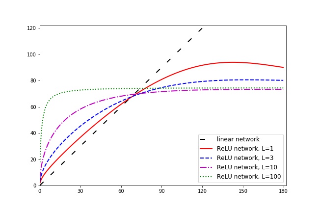
Figure 1: Model gradient angles $\phi$ vs. input angle $\theta_{in}$ (according to Theorem 4.4). Linear neural networks, of any depth $L$, always have $\bar{\phi}=\theta_{in}$, as the black dash line showed. ReLU neural networks with various depths have better data separation $\phi>\theta_{in}$ for similar data (i.e., small $\theta_{in}$). Moreover, deeper ReLU networks have better separation than shallow ones for similar data. All neural networks are infinitely wide.

The key observation is that: for relatively small input angles (say, $\theta_{in}<60^{\circ}$), the model gradient angle $\phi$ is always greater than the input angle $\theta_{in}$. This suggests that, after the mapping $\nabla f:{\mathbf{x}}\mapsto\nabla f({\mathbf{x}})$ from the input space to model gradient space, data inputs becomes more (directionally) separated, if they are similar in the input space (i.e., with small $\theta_{in}$). Comparing to the linear neural network case, where $\bar{\phi}({\mathbf{x}},{\mathbf{z}})=\theta_{in}({\mathbf{x}},{\mathbf{z}})$ as in Theorem 3.1, we see that the ReLU non-linearity results in a better angle separation $\phi({\mathbf{x}},{\mathbf{z}})>\bar{\phi}({\mathbf{x}},{\mathbf{z}})$ for similar data.

Another important observation is that: deeper ReLU networks lead to larger model gradient angles, when $\theta_{in}<60^{\circ}$. This indicates that deeper ReLU networks, which has more layers of ReLU non-linear activation, makes the model gradient more separated between inputs. Note that, in the linear network case, the depth does not affect the gradient angle $\bar{\phi}$.

We theoretically confirm these two observations in the regime of small input angle $\theta_{in}=o(1/L)$, by the following theorem.

Theorem 4.5 (Better separation with ReLU).

Consider two network inputs ${\mathbf{x}},{\mathbf{z}}\in\mathbb{R}^{d}$, with small input angle $\theta_{in}({\mathbf{x}},{\mathbf{z}})=o(1/L)$, and the ReLU network defined in Eq.(1) with $L$ hidden layers and infinite network width $m$. At the network initialization, the angle $\phi({\mathbf{x}},{\mathbf{z}})$ between the model gradients $\nabla f({\mathbf{x}})$ and $\nabla f({\mathbf{z}})$ satisfies

$$\cos\phi({\mathbf{x}},{\mathbf{z}})=\left(1-\frac{L}{2\pi}\theta_{in}+o(\theta_{in})\right)\cos\theta_{in}.$$ (11)

Noticing the negative sign within the factor $\left(1-\frac{L}{2\pi}\theta_{in}+o(\theta_{in})\right)$, we know that the factor is less than $1$ and we obtain that: $\phi({\mathbf{x}},{\mathbf{z}})>\theta_{in}({\mathbf{x}},{\mathbf{z}})=\bar{\phi}({\mathbf{x}},{\mathbf{z}})$. Noticing the depth $L$ dependence of this factor, we also get that: the deeper the ReLU network (i.e., larger $L$) is, the larger $\phi$ is, in the regime $\theta_{in}=o(1/L)$.

Remark 4.6 (Separation in distance).

Indeed, the better angle separation discussed above implies a better separation in Euclidean distance as well. This can be easily seen by recalling from Theorem 4.4 that the model gradient mapping $\nabla f$ preserves the norm (up to a universal factor $L+1$).

We also point out that, Figure 1 indicates that for large input angles (say $\theta_{in}>60^{\circ}$) the model gradient angle $\phi$ is always large (greater than $60^{\circ}$). Hence, non-similar data never become similar in the model gradient feature space.

5 Smaller condition number of NTK for ReLU network

In this section, we show both theoretically and experimentally that, with the ReLU non-linear activation function, a ReLU neural network has a smaller condition number $\kappa$ of NTK than its linear counterpart – linear neural network. Moreover, for larger network depth $L$, the NTK condition number $\kappa$ of a ReLU neural network is generically smaller.

5.1 Theoretical analysis

Theoretically, we show these findings for the following cases: two-layer ReLU network with any dataset; deep ReLU network with dataset of size $2$. In both cases, we take the infinite width limit.

Shallow ReLU neural network.

Now, let’s look at the NTK of a shallow ReLU neural network

$$f(W;{\mathbf{x}})=\frac{\sqrt{2}}{\sqrt{m}}{\mathbf{v}}^{T}\sigma(W{\mathbf{x}}).$$ (12)

Here, we fix ${\mathbf{v}}$ to random initialization and let $W$ trainable.

With the presence of the ReLU activation function, the better data separation theorem (Theorem 4.5) together with the connection between condition number and angle separation ( Proposition 2.2) suggest that the NTK of this ReLU network has a smaller condition number $\kappa$ than the Gram matrix, as well as the NTK of the linear neural network. The following theorem confirms this expectation.

Theorem 5.1.

Consider the ReLU network in Eq.(12) in the limit $m\to\infty$ and at initialization. The smallest eigenvalue $\lambda_{min}(K)$ of its NTK is larger than that of the Gram matrix: $\lambda_{min}(K)>\lambda_{min}(G)$. Moreover, the NTK condition number is less than that of the Gram matrix: $\kappa<\kappa_{0}$.

Deep ReLU neural network.

For deep ReLU network, we consider the special case where the dataset $\mathcal{D}$ consists two samples, with a small angle between their input vectors.

Theorem 5.2.

Consider the ReLU neural network $f$ as defined in Eq.(1) in the infinite width limit $m\to\infty$ and at initialization. Consider the dataset $\mathcal{D}=\{({\mathbf{x}}_{1},y_{1}),({\mathbf{x}}_{2},y_{2})\}$ with the input angle $\theta_{in}$ between ${\mathbf{x}}_{1}$ and ${\mathbf{x}}_{2}$ small, $\theta_{in}=o(1/L)$. Then, the NTK condition number $\kappa<\kappa_{0}$. Moreover, for two ReLU neural networks $f_{1}$ of depth $L_{1}$ and $f_{2}$ of depth $L_{2}$ with $L_{1}>L_{2}$, we have $\kappa_{f_{1}}<\kappa_{f_{2}}$.

This theorem also shows that a ReLU network has a better conditioned NTK than a linear model or a linear neural network. Moreover, the depth of ReLU network enhances this better conditioning. These results also confirm that the ReLU activation helps to decrease the NTK condition number.

5.2 Experimental evidence

In this subsection, we experimentally show that the phenomena of better data separation and better NTK conditioning widely happen in practice.

Dataset.

We use the following datasets: synthetic dataset, MNIST [17], FashionMNIST (f-MNIST) [34], SVHN [24] and Librispeech [26]. The synthetic data consists of $2000$ samples which are randomly drawn from a 5-dimensional Gaussian distribution with zero-mean and unit variance. The MNIST, f-MNIST and SVHN datasets are image datasets where each input is an image. The Librispeech is a speech dataset including $100$ hours of clean speeches. In the experiments, we use a subset of Librispeech with $50,000$ samples, and each input is a 768-dimensional vector representing a frame of speech audio and we follow [13] for the feature extraction.

Models.

For each of the datasets, we use a ReLU activated fully-connected neural network architecture to process. The ReLU network has $L$ hidden layers, and has $512$ neurons in each of its hidden layers. The ReLU network uses the NTK parameterization and initialization strategy (see [14]). For each dataset, we vary the network depth $L$ from $0$ to $10$. Note that $L=0$ corresponding to the linear model case. In addition, for comparison, we use a linear neural network, which has the same architecture with the ReLU network except the absence of activation function.

Results.

For each of the experimental setting, we evaluate both the smallest pairwise model gradient angle $\min_{i,j\in[n]}\phi({\mathbf{x}}_{i},{\mathbf{x}}_{j})$ and the NTK condition number $\kappa$, at the network initialization. We take $5$ independent runs over $5$ random initialization seeds, and report the average. The results are shown in Figure 2. As one can easily see from the plots, a ReLU network (depth $L=1,2,\cdots,10$) always have a better separation of data (i.e., larger smallest pairwise model gradient angle), and a better NTK conditioning (i.e., smaller NTK condition number), than its corresponding linear network (compare the solid line and dash line of the same color). Furthermore, the monotonically decreasing NTK condition number shows that a deeper ReLU network have a better conditioning of NTK.

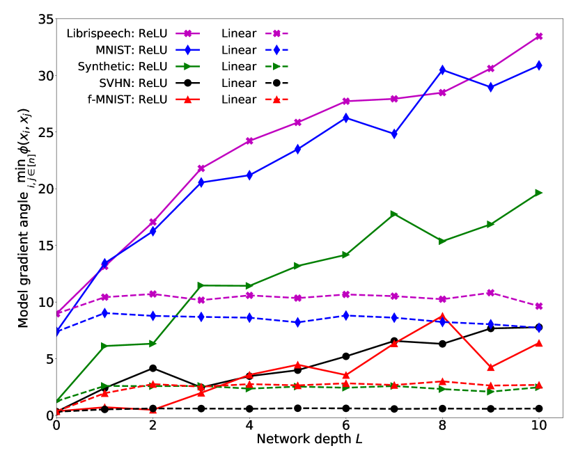
(a) Minimum $\phi$ (in degrees ^∘) vs. depth

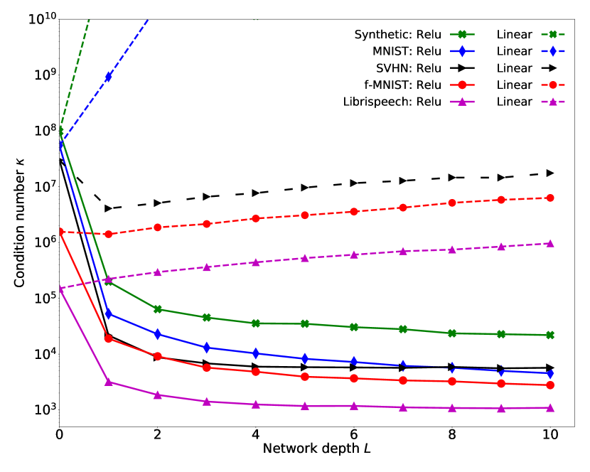
(b) NTK condition number vs. depth

Figure 2: Better separation (left) and better NTK conditioning (right) of ReLU network. Solid lines are for ReLU networks, and dash lines are for linear networks. Left: ReLU network works better in separating similar data, while linear network remains similar to a linear model. Right: ReLU network has better conditioning of NTK than linear network and linear model. Note that $L=0$ (without any hidden layer) corresponds to the case of a linear model, and the NTK in this case is the Gram matrix.

6 Optimization acceleration

Recently studies showed strong connections between the NTK condition number and the theoretical convergence rate of gradient descent algorithms on wide neural networks [8, 6, 31, 1, 37, 25, 20]. In [8, 6], the authors derived the worse case convergence rates explicitly in terms of the smallest eigenvalue of NTK $\lambda_{min}(K)$, $L({\mathbf{w}}_{t})\leq(1-\eta\lambda_{min}(K)/2)^{t}L({\mathbf{w}}_{0})$, where $L$ is the square loss function and $t$ is the time stamp of the algorithm. Later on, in [20], the NTK condition number is explicitly involved in the theoretical convergence rate:

$$L({\mathbf{w}}_{t})\leq(1-\kappa^{-1})^{t}L({\mathbf{w}}_{0}).$$ (13)

Although $\kappa$ is evaluated on the whole optimization path, all these theories used the fact that NTK is almost constant for wide neural networks and an evaluation at the initialization ${\mathbf{w}}_{0}$ is enough.

As a smaller NTK condition number (or larger smallest eigenvalue of NTK) implies a faster theoretical convergence rate, our findings suggest that: (a), wide ReLU networks have faster convergence rate than linear models and linear neural networks, and (b), deeper wide ReLU networks have faster convergence rate than shallower ones.

We experimentally verify this implication on the convergence speed. Specifically, we train the ReLU networks, with depth $L$ ranging from $1$ to $10$, for the datasets MNIST, f-MNIST and Librispeech. For all the training tasks, we use cross entropy loss as the objective function and use mini-batch stochastic gradient descent (SGD) of batch size $500$ to optimize. For each task, we find its optimal learning rate by grid search. On MNIST and f-MNIST, we train $500$ epochs, and on Librispeech, we training $2000$ epochs.

The curves of training loss against epochs are shown in Figure 3. We observe that, for all these datasets, a deeper ReLU network always converges faster than shallower ones. This is consistent with the theoretical prediction that the deeper ReLU network, which has smaller NTK condition number, has faster theoretical convergence rate.

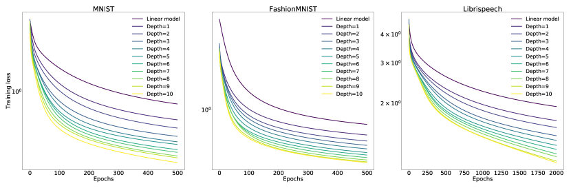
Figure 3: Training curve of ReLU networks with different depths. On each of these datasets, we see that deeper ReLU network always converges faster than shallower ones.

7 Conclusion and discussions

In this work, we showed the key role that ReLU (as a non-linear activation function) played in data separation: for any two inputs that are “directionally” close (small $\theta_{in}$) in the original input space, a ReLU activated neural network makes them better separated in the model gradient feature space ($\phi>\theta_{in}$), while a linear neural network, which has no non-linear activation, keeps the same separation ($\bar{\phi}=\theta_{in}$). As a consequence, the NTK condition number $\kappa$ for the ReLU neural network is smaller than those for the linear model and linear neural networks. Moreover, we showed that the NTK condition number $\kappa$ is further decreased if the ReLU network is going deeper. The smaller NTK condition number suggests a faster gradient descent convergence rate for deep ReLU neural network.

Finite network width.

Our theoretical analysis is based the setting of infinite network width. We note that, for finite network width and at network initialization, the analysis only differs by a zero-mean noisy term, wherever we took the limit $m\to\infty$. This noisy term scales down to $0$ as the network width increases. We believe our main results still hold for finite but large network width.

Infinite depth.

In this work, we focused on the finite depth scenario which is the more interesting case from a practical point of view. Our small angle regime analysis (Corollary 4.3, Theorem 4.5 and 5.2) do not directly extend to the infinite depth case. But, as Theorem 4.4 and Figure 1 indicate, the $\phi(\theta_{in})$ function seems to converge to a step function when $L\to\infty$, which implies orthogonality between each pair of model gradient vectors, hence a NTK condition number being $1$. This is consistent with the prior knowledge that NTK converges to $1$ in the infinite depth limit [28].

Other activation functions.

In this work, we focused on ReLU, which is the mostly used activation function in practice. We believe similar results also hold for other non-linear activation functions. We leave this direction as a future work.

Appendix A Properties of function $g$

Recall that the function $g:[0,\pi)\to[0,\pi)$ is defined as

$$g(z)=\arccos\left(\frac{\pi-z}{\pi}\cos z+\frac{1}{\pi}\sin z\right),$$ (14)

Figure 4 shows the plot of this function. From the plot, we can easily find the following properties.

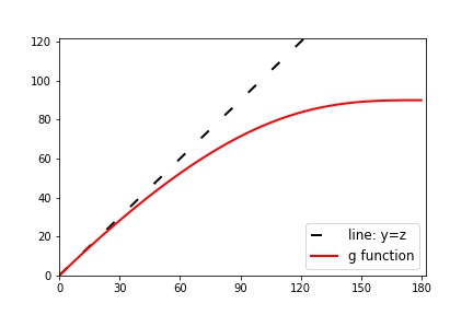
Figure 4: Curve of the function $g(\theta)$. As can be seen, $g(\theta)$ is monotonic, and is approximately the identity function $y=\theta$ in the small angle region ($\theta\ll 90^{\circ}$).

Proposition A.1 (Properties of $g$).

The function $g$ defined in Eq.(8) has the following properties:

1. $g$ is a monotonically increasing function;

2. $g(z)\leq z$, for all $z\in[0,\pi)$; and $g(z)=z$ if and only if $z=0$;

3. for any $z\in[0,\pi)$, the sequence $\{g^{l}(z)\}_{l=1}^{\infty}$ is monotonically decreasing, and has the limit $\lim_{l\to\infty}g^{l}(z)=0$.

It is worth to note that the last property of $g$ function immediately implies the collapse of embedding vectors from different inputs in the infinite depth limit $L\to\infty$. This embedding collapse has been observed in prior works [27, 30] (although by different type of analysis) and has been widely discussed in the literature of Edge of Chaos.

Theorem A.2.

Consider the same ReLU neural network as in Theorem 4.1. Given any two inputs ${\mathbf{x}},{\mathbf{z}}\in\mathbb{R}^{d}$, the sequence of angles between their $l$-embedding vectors, $\{\theta^{(l)}({\mathbf{x}},{\mathbf{z}})\}_{l=1}^{L}$, is monotonically decreasing. Moreover, in the limit of infinite depth,

$$\lim_{L\to\infty}\theta^{(L)}({\mathbf{x}},{\mathbf{z}})=0,$$ (15)

and there exists a vector $\alpha$ such that, for any input ${\mathbf{x}}$, the last layer $L$-embedding

$$\alpha^{(L)}({\mathbf{x}})=\|{\mathbf{x}}\|\alpha.$$ (16)

Proof of Proposition A.1.

Part $1$. First, we consider the auxiliary function $\tilde{g}(z)=\frac{\pi-z}{\pi}\cos z+\frac{1}{\pi}\sin z$. We see that

$$\frac{d\tilde{g}(z)}{dz}=-\left(1-\frac{z}{\pi}\right)\sin z\leq 0,~{}~{}\forall z\in[0,\pi).$$

Hence, $\tilde{g}(z)$ is monotonically decreasing on $[0,\pi)$. Combining with the monotonically decreasing nature of the $\arccos$ function, we get that $g$ is monotonically increasing.

Part $2$. It suffices to prove that $\cos z\leq\tilde{g}(z)$ and that the equality holds only at $z=0$. For $z=0$, it is easy to check that $\cos z=\tilde{g}(z)$, as both $z$ and $\sin z$ are zero. For $z\in(0,\pi/2)$, noting that $\tan z-z>0$, we have

$$\tilde{g}(z)=\frac{\pi-z}{\pi}\cos z+\frac{1}{\pi}\sin z=\cos z+\frac{1}{\pi}\left(-z+\tan z\right)\cos z>\cos z.$$ (17)

For $z=\pi/2$, we have $\cos\pi/2=0<1/\pi=\tilde{g}(\pi/2)$. For $z\in(\pi/2,\pi)$, we have the same relation as in Eq.(17). The only differences are that, in this case, $\cos z<0$ and $\tan z-z<0$. Therefore, we still get $\tilde{g}(z)>\cos z$ for $z\in(\pi/2,\pi)$.

Part 3. From part $2$, we see that $g(z)<z$ for all $z\in(0,\pi)$. Hence, for any $l$, $g^{l+1}(z)<g^{l}(z)$. Moreover, since $z=0$ is the only fixed point such that $g(z)=z$, in the limit $l\to\infty$, $g^{l}(z)\to 0$. ∎

Appendix B Proof of Proposition 2.2

Proof.

Consider the matrix $B$ and the $n$ vectors ${\mathbf{b}}_{k}\triangleq B_{k\cdot}$, $k\in[n]$. The smallest singular value square of matrix $B$ is defined as

$$\sigma_{min}^{2}(B)=\min_{{\mathbf{v}}\neq 0}\frac{{\mathbf{v}}^{T}BB^{T}{\mathbf{v}}}{{\mathbf{v}}^{T}{\mathbf{v}}}=\min_{{\mathbf{v}}\neq 0}\frac{\|\sum_{k}v_{k}{\mathbf{b}}_{k}\|^{2}}{\|{\mathbf{v}}\|^{2}}.$$

Since the angle $\phi$ between ${\mathbf{b}}_{i}=B_{i\cdot}$ and ${\mathbf{b}}_{j}=B_{j\cdot}$ is small, let ${\mathbf{v}}^{\prime}$ be the vector such that $v^{\prime}_{i}=\|{\mathbf{b}}_{j}\|$, $v^{\prime}_{j}=-\|{\mathbf{b}}_{i}\|$ and $v^{\prime}_{k}=0$ for all $k\neq i,j$. Then

$$\sigma_{min}^{2}(B) \leq\frac{\|\sum_{k}v^{\prime}_{k}{\mathbf{b}}_{k}\|^{2}}{\|{\mathbf{v}}^{\prime}\|^{2}}=\left\|\frac{\|{\mathbf{b}}_{j}\|}{\sqrt{\|{\mathbf{b}}_{i}\|^{2}+\|{\mathbf{b}}_{j}\|^{2}}}{\mathbf{b}}_{i}-\frac{\|{\mathbf{b}}_{i}\|}{\sqrt{\|{\mathbf{b}}_{i}\|^{2}+\|{\mathbf{b}}_{j}\|^{2}}}{\mathbf{b}}_{j}\right\|^{2}$$

$$=\frac{2\|{\mathbf{b}}_{i}\|^{2}\|{\mathbf{b}}_{j}\|^{2}}{\|{\mathbf{b}}_{i}\|^{2}+\|{\mathbf{b}}_{j}\|^{2}}(1-\cos\phi)$$

$$=\frac{\|{\mathbf{b}}_{i}\|^{2}\|{\mathbf{b}}_{j}\|^{2}}{\|{\mathbf{b}}_{i}\|^{2}+\|{\mathbf{b}}_{j}\|^{2}}\phi^{2}+O(\phi^{4}).$$

Since $A=BB^{T}$, the smallest eigenvalue $\lambda_{min}(A)$ of $A$ is the same as $\sigma_{min}^{2}(B)$.

On the other hand, the largest eigenvalue $\lambda_{max}(A)$ of matrix $A$ is lower bounded by tr$(A)/n$. Note that the diagonal entries $A_{kk}=\|{\mathbf{b}}_{k}\|$. Hence, $c\leq\lambda_{max}(A)\leq C$. Therefore, the condition number $\kappa=\lambda_{max}(A)/\lambda_{min}(A)=\Omega(1/\phi^{2})$. ∎

Appendix C Proofs of Theorems for linear neural network

C.1 Proof of Theorem 3.1

Proof.

First of all, we provide a useful lemma.

Lemma C.1.

Consider a matrix $A\in\mathbb{R}^{m\times d}$, with each entry of $A$ is i.i.d. drawn from $\mathcal{N}(0,1)$. In the limit of $m\to\infty$,

$$\frac{1}{m}A^{T}A\to I_{d\times d},~{}~{}\textrm{in probability.}$$ (18)

We first consider the embedding vectors $\bar{\alpha}^{(l)}$ and the embedding angles $\bar{\theta}^{(l)}$. By definition in Eq.(3), we have, for all $l\in[L]$ and input ${\mathbf{x}}\in\mathbb{R}^{d}$,

$$\bar{\alpha}^{(l)}({\mathbf{x}})=\frac{1}{m^{l/2}}W^{(l)}W^{(l-1)}\cdots W^{(1)}{\mathbf{x}}.$$ (19)

Note that at the network initialization entries of $W^{(l)}$ are i.i.d. and follows $\mathcal{N}(0,1)$. Hence, the inner product

$$\langle\bar{\alpha}^{(l)}({\mathbf{x}}),\bar{\alpha}^{(l)}({\mathbf{z}})\rangle =\frac{1}{m^{l}}{\mathbf{x}}^{T}W^{(1)T}\cdots W^{(l-1)T}W^{(l)T}W^{(l)}W^{(l-1)}\cdots W^{(1)}{\mathbf{z}}\overset{(a)}{=}{\mathbf{x}}^{T}{\mathbf{z}},$$

where in step (a) we recursively applied Lemma C.1 $l$ times. Putting ${\mathbf{z}}={\mathbf{x}}$, we get $\|\bar{\alpha}^{(l)}({\mathbf{x}})\|=\|{\mathbf{x}}\|$, for all $l\in[L]$. By the definition of embedding angles, it is easy to check that $\bar{\theta}^{(l)}({\mathbf{x}},{\mathbf{z}})=\theta_{in}({\mathbf{x}},{\mathbf{z}})$, for all $l\in[L]$.

Now, we consider the model gradient $\nabla\bar{f}$ and the model gradient angle $\bar{\phi}$. As we consider the model gradient only at network initialization, we don’t explicitly write out the dependence on ${\mathbf{w}}_{0}$, and we write $\nabla\bar{f}({\mathbf{w}}_{0},{\mathbf{x}})$ simply as $\nabla\bar{f}({\mathbf{x}})$. The model gradient $\nabla\bar{f}$ can be decomposed as

$$\nabla\bar{f}({\mathbf{x}})=(\nabla_{1}\bar{f}({\mathbf{x}}),\nabla_{2}\bar{f}({\mathbf{x}}),\cdots,\nabla_{L+1}\bar{f}({\mathbf{x}})),~{}~{}with~{}\nabla_{l}\bar{f}({\mathbf{x}})=\frac{\partial\bar{f}({\mathbf{x}})}{\partial W^{(l)}},\forall l\in[L+1].$$ (20)

Hence, the inner product

$$\langle\nabla\bar{f}({\mathbf{x}}),\nabla\bar{f}({\mathbf{z}})\rangle =\sum_{l=1}^{L+1}\langle\nabla_{l}\bar{f}({\mathbf{x}}),\nabla_{l}\bar{f}({\mathbf{z}})\rangle,$$

and for all $l\in[l+1]$,

$$\langle\nabla_{l}\bar{f}({\mathbf{x}}),\nabla_{l}\bar{f}({\mathbf{z}})\rangle =\langle\bar{\alpha}^{(l-1)}({\mathbf{x}}),\bar{\alpha}^{(l-1)}({\mathbf{z}})\rangle\cdot\langle\prod_{l^{\prime}=l+1}^{L+1}\frac{1}{\sqrt{m}}W^{(l^{\prime})T},\prod_{l^{\prime}=l+1}^{L+1}\frac{1}{\sqrt{m}}W^{(l^{\prime})T}\rangle\overset{(b)}{=}{\mathbf{x}}^{T}{\mathbf{z}}.$$

Here in step (b), we again applied Lemma C.1. Therefore,

$$\langle\nabla\bar{f}({\mathbf{x}}),\nabla\bar{f}({\mathbf{z}})\rangle=(L+1){\mathbf{x}}^{T}{\mathbf{z}}.$$ (21)

Putting ${\mathbf{z}}={\mathbf{x}}$, we get $\|\nabla f({\mathbf{x}})\|=(L+1)\|{\mathbf{x}}\|$. By the definition of model gradient angle, it is easy to check that $\bar{\phi}({\mathbf{x}},{\mathbf{z}})=\theta_{in}({\mathbf{x}},{\mathbf{z}})$. ∎

Appendix D Proofs of Theorems for ReLU network

D.1 Preliminary results

Before the proofs, we introduce some useful notations and lemmas.

Given a vector ${\mathbf{v}}\in\mathbb{R}^{p}$, we define the following diagonal indicator matrix:

$$\mathbb{I}_{\{{\mathbf{v}}\geq 0\}}=\mathsf{diag}\left(\mathbb{I}_{\{v_{1}\geq 0\}},\mathbb{I}_{\{v_{2}\geq 0\}},\cdots,\mathbb{I}_{\{v_{p}\geq 0\}}\right),$$ (22)

with

$$\mathbb{I}_{\{v_{i}\geq 0\}}=\left\{\begin{array}[]{ll}1&v_{i}\geq 0,\\ 0&v_{i}<0.\end{array}\right.$$

Lemma D.1.

Consider two vectors ${\mathbf{v}}_{1},{\mathbf{v}}_{2}\in\mathbb{R}^{p}$ and a $p$-dimensional random vector ${\mathbf{w}}\sim\mathcal{N}(0,I_{p\times p})$. Denote $\theta$ as the angle between ${\mathbf{v}}_{1}$ and ${\mathbf{v}}_{2}$, i.e., $\cos\theta=\frac{\langle{\mathbf{v}}_{1},{\mathbf{v}}_{2}\rangle}{\|{\mathbf{v}}_{1}\|\|{\mathbf{v}}_{2}\|}$. Then, the probability

$$\mathbb{P}[({\mathbf{w}}^{T}{\mathbf{v}}_{1}\geq 0)\wedge({\mathbf{w}}^{T}{\mathbf{v}}_{2}\geq 0)]=\frac{1}{2}-\frac{\theta}{2\pi}.$$ (23)

Lemma D.2.

Consider two arbitrary vectors ${\mathbf{v}}_{1},{\mathbf{v}}_{2}\in\mathbb{R}^{p}$ and a random matrix $W\in\mathbb{R}^{q\times p}$ with entries $W_{ij}$ i.i.d. drawn from $\mathcal{N}(0,1)$. Denote $\theta$ as the angle between ${\mathbf{v}}_{1}$ and ${\mathbf{v}}_{2}$, and define ${\mathbf{u}}_{1}=\frac{\sqrt{2}}{\sqrt{q}}\sigma(W{\mathbf{v}}_{1})$ and ${\mathbf{u}}_{2}=\frac{\sqrt{2}}{\sqrt{q}}\sigma(W{\mathbf{v}}_{2})$. Then, in the limit of $q\to\infty$,

$$\langle{\mathbf{u}}_{1},{\mathbf{u}}_{2}\rangle=\frac{1}{\pi}\left((\pi-\theta)\cos\theta+\sin\theta\right)\|{\mathbf{v}}_{1}\|\|{\mathbf{v}}_{2}\|.$$ (24)

Lemma D.3.

Consider two arbitrary vectors ${\mathbf{v}}_{1},{\mathbf{v}}_{2}\in\mathbb{R}^{p}$ and two random matrices $U\in\mathbb{R}^{s\times q}$ and $W\in\mathbb{R}^{q\times p}$, where all entries $U_{ij}$, $i\in[s]$ and $j\in[q]$, and $W_{kl}$, $k\in[q]$ and $l\in[p]$, are i.i.d. drawn from $\mathcal{N}(0,1)$. Denote $\theta$ as the angle between ${\mathbf{v}}_{1}$ and ${\mathbf{v}}_{2}$, and define matrices $A_{1}=\frac{\sqrt{2}}{\sqrt{q}}U\mathbb{I}_{\{W{\mathbf{v}}_{1}\geq 0\}}$ and $A_{2}=\frac{\sqrt{2}}{\sqrt{q}}U\mathbb{I}_{\{W{\mathbf{v}}_{2}\geq 0\}}$. Then, in the limit of $q\to\infty$, the matrix

$$A_{1}A_{2}^{T}=\frac{\pi-\theta}{\pi}I_{s\times s}.$$ (25)

D.2 Proof of Theorem 4.1

Proof.

Consider an arbitrary layer $l\in[L]$ of the ReLU neural network $f$ at initialization. Given two arbitrary network inputs ${\mathbf{x}},{\mathbf{z}}\in\mathbb{R}^{d}$, the inputs to the $l$-th layer are $\alpha^{(l-1)}({\mathbf{x}}))$ and $\alpha^{(l-1)}({\mathbf{z}}))$, respectively.

By definition, we have

$$\alpha^{(l)}({\mathbf{x}})=\sqrt{\frac{2}{m}}\sigma\left(W^{(l)}\alpha^{(l-1)}({\mathbf{x}})\right),~{}~{}\alpha^{(l)}({\mathbf{z}})=\sqrt{\frac{2}{m}}\sigma\left(W^{(l)}\alpha^{(l-1)}({\mathbf{z}})\right),$$ (26)

with entries of $W^{(l)}$ being i.i.d. drawn from $\mathcal{N}(0,1)$. Recall that, by definition, the angle between $\alpha^{(l-1)}({\mathbf{x}}))$ and $\alpha^{(l-1)}({\mathbf{z}}))$ is $\theta^{(l-1)}({\mathbf{x}},{\mathbf{z}})$. Applying Lemma D.2, we immediately have the inner product

$$\langle\alpha^{(l)}({\mathbf{z}}),\alpha^{(l)}({\mathbf{x}})\rangle=\frac{1}{\pi}\left((\pi-\theta^{(l-1)}({\mathbf{x}},{\mathbf{z}}))\cos\theta^{(l-1)}({\mathbf{x}},{\mathbf{z}})+\sin\theta^{(l-1)}({\mathbf{x}},{\mathbf{z}})\right)\|\alpha^{(l-1)}({\mathbf{x}})\|\|\alpha^{(l-1)}({\mathbf{z}})\|.$$ (27)

In the special case of ${\mathbf{x}}={\mathbf{z}}$, we have $\theta^{(l-1)}({\mathbf{x}},{\mathbf{z}})=0$, and obtain from the above equation that

$$\|\alpha^{(l)}({\mathbf{x}})\|^{2}=\|\alpha^{(l-1)}({\mathbf{x}})\|^{2}.$$ (28)

Apply Eq.(28) back to Eq.(27), we also get

$$\cos\theta^{(l)}({\mathbf{x}},{\mathbf{z}})=\frac{\langle\alpha^{(l)}({\mathbf{z}}),\alpha^{(l)}({\mathbf{x}})\rangle}{\|\alpha^{(l)}({\mathbf{x}})\|\|\alpha^{(l)}({\mathbf{z}})\|}=\frac{1}{\pi}\left((\pi-\theta^{(l-1)}({\mathbf{x}},{\mathbf{z}}))\cos\theta^{(l-1)}({\mathbf{x}},{\mathbf{z}})+\sin\theta^{(l-1)}({\mathbf{x}},{\mathbf{z}})\right).$$ (29)

∎

D.3 Proof of Corollary 4.3

Proof.

By Theorem 4.1, we have that

$$\cos\theta^{(l)}({\mathbf{x}},{\mathbf{z}}) =\left(1-\frac{\theta^{(l-1)}({\mathbf{x}},{\mathbf{z}})}{\pi}\right)\cos\theta^{(l-1)}({\mathbf{x}},{\mathbf{z}})+\frac{1}{\pi}\sin\theta^{(l-1)}({\mathbf{x}},{\mathbf{z}})$$

$$=\cos\theta^{(l-1)}({\mathbf{x}},{\mathbf{z}})\left(1+\frac{1}{\pi}\left(\tan\theta^{(l-1)}({\mathbf{x}},{\mathbf{z}})-\theta^{(l-1)}({\mathbf{x}},{\mathbf{z}})\right)\right)$$

$$=\cos\theta^{(l-1)}({\mathbf{x}},{\mathbf{z}})\left(1+\frac{1}{3\pi}(\theta^{(l-1)}({\mathbf{x}},{\mathbf{z}}))^{3}+o\left((\theta^{(l-1)}({\mathbf{x}},{\mathbf{z}}))^{3}\right)\right).$$

Noting that the Taylor expansion of the $\cos$ function at zero is $\cos z=1-\frac{1}{2}z^{2}+o(z^{3})$, one can easily check that, for all $l\in[L]$,

$$\theta^{(l)}({\mathbf{x}},{\mathbf{z}})=\theta^{(l-1)}({\mathbf{x}},{\mathbf{z}})-\frac{1}{3\pi}(\theta^{(l-1)}({\mathbf{x}},{\mathbf{z}}))^{2}+o\left((\theta^{(l-1)}({\mathbf{x}},{\mathbf{z}}))^{2}\right).$$ (30)

Note that $\theta^{(l)}({\mathbf{x}},{\mathbf{z}})\leq\theta^{(l-1)}({\mathbf{x}},{\mathbf{z}})=o(1/L)$. Iteratively apply the above equation, one gets, for all $l\in[L]$, if $\theta^{(0)}({\mathbf{x}},{\mathbf{z}})=o(1/L)$,

$$\theta^{(l)}({\mathbf{x}},{\mathbf{z}})=\theta^{(0)}({\mathbf{x}},{\mathbf{z}})-\frac{l}{3\pi}(\theta^{(0)}({\mathbf{x}},{\mathbf{z}}))^{2}+o\left((\theta^{(0)}({\mathbf{x}},{\mathbf{z}}))^{2}\right).$$ (31)

∎

D.4 Proof of Theorem 4.4

Proof.

The model gradient $\nabla f({\mathbf{x}})$ is composed of the components $\nabla_{l}f({\mathbf{x}})\triangleq\frac{\partial f}{\partial W^{l}}$, for $l\in[L+1]$. Each such component has the following expression: for $l\in[L+1]$

$$\nabla_{l}f({\mathbf{x}})=\alpha^{(l-1)}({\mathbf{x}})\delta^{(l)}({\mathbf{x}}),$$ (32)

where

$$\delta^{(l)}({\mathbf{x}})=\left(\frac{2}{m}\right)^{\frac{L-l+1}{2}}W^{(L+1)}\mathbb{I}_{\{\tilde{\alpha}^{(L)}({\mathbf{x}})\geq 0\}}W^{(L)}\mathbb{I}_{\{\tilde{\alpha}^{(L-1)}({\mathbf{x}})\geq 0\}}\cdots W^{(l+1)}\mathbb{I}_{\{\tilde{\alpha}^{(l)}({\mathbf{x}})\geq 0\}}.$$ (33)

Note that in Eq.(32), $\nabla_{l}f({\mathbf{x}})$ is an outer product of a column vector $\alpha^{(l-1)}({\mathbf{x}})\in\mathbb{R}^{m_{l-1}\times 1}$ ($m_{l-1}=d$ if $l=1$, and $m_{l-1}=m$ otherwise) and a row vector $\delta^{(l)}({\mathbf{x}})\in\mathbb{R}^{1\times m_{l}}$ ($m_{l}=1$ if $l=L+1$, and $m_{l}=m$ otherwise).

First, we consider the inner product $\langle\nabla_{l}f({\mathbf{z}}),\nabla_{l}f({\mathbf{x}})\rangle$, for $l\in[L+1]$. By Eq.(32), we have

$$\langle\nabla_{l}f({\mathbf{z}}),\nabla_{l}f({\mathbf{x}})\rangle=\langle\delta^{(l)}({\mathbf{z}}),\delta^{(l)}({\mathbf{x}})\rangle\cdot\langle\alpha^{(l-1)}({\mathbf{z}}),\alpha^{(l-1)}({\mathbf{x}})\rangle.$$ (34)

For $\langle\alpha^{(l-1)}({\mathbf{z}}),\alpha^{(l-1)}({\mathbf{x}})\rangle$, applying Theorem 4.1 and Corollary 4.2, we have

$$\langle\alpha^{(l-1)}({\mathbf{z}}),\alpha^{(l-1)}({\mathbf{x}})\rangle=\|{\mathbf{x}}\|\|{\mathbf{z}}\|\cos\theta^{(l-1)}({\mathbf{x}},{\mathbf{z}}).$$ (35)

For $\langle\delta^{(l)}({\mathbf{z}}),\delta^{(l)}({\mathbf{x}})\rangle$, by definition Eq.(33), we have

$$\langle\delta^{(l)}({\mathbf{z}}),\delta^{(l)}({\mathbf{x}})\rangle$$

$$=\left(\frac{2}{m}\right)^{L-l+1}W^{(L+1)}\mathbb{I}_{\{\tilde{\alpha}^{(L)}({\mathbf{x}})\geq 0\}}\cdots\underbrace{W^{(l+1)}\mathbb{I}_{\{\tilde{\alpha}^{(l)}({\mathbf{x}})\geq 0,\tilde{\alpha}^{(l)}({\mathbf{z}})\geq 0\}}W^{(l+1)T}}_{A}\cdots\mathbb{I}_{\{\tilde{\alpha}^{(L)}({\mathbf{z}})\geq 0\}}W^{(L+1)T}$$

Recalling that $\tilde{\alpha}^{(l)}=W^{(l)}\tilde{\alpha}^{(l-1)}$ and applying Lemma D.3 on the the term $A$ above, we obtain

$$\langle\delta^{(l)}({\mathbf{z}}),\delta^{(l)}({\mathbf{x}})\rangle =\frac{\pi-\theta^{(l-1)}({\mathbf{x}},{\mathbf{z}})}{\pi}\langle\delta^{(l+1)}({\mathbf{z}}),\delta^{(l+1)}({\mathbf{x}})\rangle.$$

Recursively applying the above formula for $l^{\prime}=l,l+1,\cdots,L$, and noticing that $\delta^{(L+1)}=1$, we have

$$\langle\delta^{(l)}({\mathbf{z}}),\delta^{(l)}({\mathbf{x}})\rangle=\prod_{l^{\prime}=l-1}^{L+1}\left(1-\frac{\theta^{(l^{\prime})}({\mathbf{x}},{\mathbf{z}})}{\pi}\right).$$ (36)

Combining Eq.(34), (35) and (36), we have

$$\langle\nabla_{l}f({\mathbf{z}}),\nabla_{l}f({\mathbf{x}})\rangle=\|{\mathbf{x}}\|\|{\mathbf{z}}\|\cos\theta^{(l-1)}({\mathbf{x}},{\mathbf{z}})\prod_{l^{\prime}=l-1}^{L-1}\left(1-\frac{\theta^{(l^{\prime})}({\mathbf{x}},{\mathbf{z}})}{\pi}\right).$$ (37)

For the inner product between the full model gradients, we have

$$\langle\nabla f({\mathbf{z}}),\nabla f({\mathbf{x}})\rangle=\sum_{l=1}^{L+1}\langle\nabla_{l}f({\mathbf{z}}),\nabla_{l}f({\mathbf{x}})\rangle=\|{\mathbf{x}}\|\|{\mathbf{z}}\|\sum_{l=0}^{L}\left[\cos\theta^{(l)}({\mathbf{x}},{\mathbf{z}})\prod_{l^{\prime}=l}^{L-1}\left(1-\frac{\theta^{(l^{\prime})}({\mathbf{x}},{\mathbf{z}})}{\pi}\right)\right].$$ (38)

Putting ${\mathbf{x}}={\mathbf{z}}$ in the above equation, we have $\theta^{(l)}({\mathbf{x}},{\mathbf{z}})=0$ for all $l\in[L]$, and obtain

$$\|\nabla f({\mathbf{x}})\|^{2}=\|{\mathbf{x}}\|^{2}\cdot(L+1).$$ (39)

Hence, we have

$$\cos\phi({\mathbf{x}},{\mathbf{z}})=\frac{\langle\nabla f({\mathbf{z}}),\nabla f({\mathbf{x}})\rangle}{\|\nabla f({\mathbf{x}})\|\|\nabla f({\mathbf{z}})\|}=\frac{1}{L+1}\sum_{l=0}^{L}\left[\cos\theta^{(l)}({\mathbf{x}},{\mathbf{z}})\prod_{l^{\prime}=l}^{L-1}(1-\theta^{(l^{\prime})}({\mathbf{x}},{\mathbf{z}})/\pi)\right].$$ (40)

∎

D.5 Proof of Theorem 4.5

Proof.

For simplicity of notation, we don’t explicitly write out the dependent on the inputs ${\mathbf{x}},{\mathbf{z}}$, and write $\theta^{(l)}\triangleq\theta^{(l)}({\mathbf{x}},{\mathbf{z}})$, and $\phi\triangleq\phi({\mathbf{x}},{\mathbf{z}})$. We start the proof with the relation provided by Theorem 4.4.

$$\cos\phi({\mathbf{x}},{\mathbf{z}}) =\frac{1}{L+1}\sum_{l=0}^{L}\left[\cos\theta^{(l)}\prod_{l^{\prime}=l}^{L-1}(1-\theta^{(l^{\prime})}/\pi)\right]$$

$$\overset{(a)}{=}\frac{1}{L+1}\sum_{l=0}^{L}\left[\cos\theta^{(0)}\prod_{l^{\prime}=0}^{l-1}\left(1+\frac{1}{\pi}\tan\theta^{(l^{\prime})}-\frac{1}{\pi}\theta^{(l^{\prime})}\right)\prod_{l^{\prime}=l}^{L-1}(1-\theta^{(l^{\prime})}/\pi)\right]$$

$$\overset{(b)}{=}\frac{1}{L+1}\sum_{l=0}^{L}\left[\cos\theta^{(0)}\prod_{l^{\prime}=0}^{l-1}\left(1+\frac{1}{3\pi}(\theta^{(l^{\prime})})^{3}+o(\theta^{(l^{\prime})})^{3}\right)\prod_{l^{\prime}=l}^{L-1}(1-\theta^{(l^{\prime})}/\pi)\right]$$

$$\overset{(c)}{=}\frac{\cos\theta^{(0)}}{L+1}\sum_{l=0}^{L}\left[\prod_{l^{\prime}=0}^{l-1}\left(1+\frac{1}{3\pi}(\theta^{(0)})^{3}+o(\theta^{(0)})^{3}\right)\prod_{l^{\prime}=l}^{L-1}\left(1-\frac{1}{\pi}\theta^{(0)}+\frac{l^{\prime}}{3\pi^{2}}(\theta^{(0)})^{2}+o((\theta^{(0)})^{2})\right)\right]$$

$$=\frac{\cos\theta^{(0)}}{L+1}\sum_{l=0}^{L}\left(1-\frac{L-l}{\pi}\theta^{(0)}+\frac{(L-l)(2L-l-2)}{3\pi^{2}}(\theta^{(0)})^{2}+o((\theta^{(0)})^{2})\right)$$

$$=\cos\theta^{(0)}\left(1-\frac{L}{2}\theta^{(0)}+o(\theta^{(0)})\right).$$

∎

D.6 Proof of Theorem 5.1

Proof.

For this shallow ReLU network, the model gradient, for an arbitrary input ${\mathbf{x}}$, is written as

$$\nabla f({\mathbf{x}})={\mathbf{x}}\delta({\mathbf{x}})\in\mathbb{R}^{d\times m},$$ (41)

where $\delta({\mathbf{x}})\in\mathbb{R}^{1\times m}$ has the following expression

$$\delta({\mathbf{x}})=\sqrt{\frac{2}{m}}{\mathbf{v}}^{T}\mathbb{I}_{\{W{\mathbf{x}}\geq 0\}}.$$

At initialization, $W$ is a random matrix. Utilizing Lemma D.3, it is easy to check that $\|\delta({\mathbf{x}})\|=1$ for all input ${\mathbf{x}}$ in the infinite width limit.

Recall that the NTK $K=FF^{T}$, where the gradient feature matrix $F$ consist of the gradient feature vectors $\nabla f({\mathbf{x}})$ for all ${\mathbf{x}}$ for the dataset. Hence, the smallest eigenvalue $\lambda_{min}(K)$ satisfies

$$\lambda_{min}(K) =\min_{{\mathbf{u}}\neq 0}\frac{{\mathbf{u}}^{T}K{\mathbf{u}}}{\|{\mathbf{u}}\|^{2}}=\min_{{\mathbf{u}}\neq 0}\frac{\left\|\sum_{i=1}^{n}u_{i}\nabla f({\mathbf{x}}_{i})\right\|^{2}}{\sum_{i=1}^{n}u_{i}^{2}}$$

$$=\min_{{\mathbf{u}}\neq 0}\frac{\sum_{j=1}^{m}\|\sum_{i=1}^{n}u_{i}\delta_{j}({\mathbf{x}}_{i}){\mathbf{x}}_{i}\|^{2}}{\sum_{i=1}^{n}u_{i}^{2}}$$

$$=\min_{{\mathbf{u}}\neq 0}\sum_{j=1}^{m}\frac{\sum_{i=1}^{n}(u_{i}\delta_{j}({\mathbf{x}}_{i}))^{2}}{\sum_{i=1}^{n}u_{i}^{2}}\frac{\|\sum_{i=1}^{n}u_{i}\delta_{j}({\mathbf{x}}_{i}){\mathbf{x}}_{i}\|^{2}}{\sum_{i=1}^{n}(u_{i}\delta_{j}({\mathbf{x}}_{i}))^{2}}$$

$$\overset{(a)}{>}\min_{{\mathbf{u}}\neq 0}\sum_{j=1}^{m}\frac{\sum_{i=1}^{n}(u_{i}\delta_{j}({\mathbf{x}}_{i}))^{2}}{\sum_{i=1}^{n}u_{i}^{2}}\lambda_{min}(G).$$ (42)

In the inequality $(a)$ above, we made the following treatment: for each fixed $j$, we consider $u_{i}\delta_{j}({\mathbf{x}}_{i})$ as the $i$-th component of a vector ${\mathbf{u}}^{\prime}_{j}$; by definition, the minimum eigenvalue of Gram matrix

$$\lambda_{min}(G)=\min_{{\mathbf{u}}^{\prime}\neq 0}({\mathbf{u}}^{\prime})^{T}G{\mathbf{u}}^{\prime}/\|{\mathbf{u}}^{\prime}\|^{2}\leq({\mathbf{u}}^{\prime}_{j})^{T}G{\mathbf{u}}^{\prime}_{j}/\|{\mathbf{u}}^{\prime}_{j}\|^{2},~{}~{}\forall j;$$ (43)

moreover, this $\leq$ inequality becomes equality, if and only if all ${\mathbf{u}}^{\prime}_{j}$ are the same and equal to $\arg\min_{{\mathbf{u}}^{\prime}\neq 0}({\mathbf{u}}^{\prime})^{T}G{\mathbf{u}}^{\prime}/\|{\mathbf{u}}^{\prime}\|^{2}$. As easy to see, for different $j$, ${\mathbf{u}}^{\prime}_{j}$ are different, hence only the strict inequality $<$ holds in step $(a)$.

Continuing from Eq.(42), we have

$$\lambda_{min}(K) >\min_{{\mathbf{u}}\neq 0}\sum_{j=1}^{m}\frac{\sum_{i=1}^{n}(u_{i}\delta_{j}({\mathbf{x}}_{i}))^{2}}{\sum_{i=1}^{n}u_{i}^{2}}\lambda_{min}(G)$$

$$=\min_{{\mathbf{u}}\neq 0}\frac{\sum_{i=1}^{n}u_{i}^{2}\|\delta({\mathbf{x}}_{i})\|^{2}}{\sum_{i=1}^{n}u_{i}^{2}}\lambda_{min}(G)$$

$$=\min_{{\mathbf{u}}\neq 0}\frac{\sum_{i=1}^{n}u_{i}^{2}}{\sum_{i=1}^{n}u_{i}^{2}}\lambda_{min}(G)=\lambda_{min}(G).$$

Therefore, we showed that $\lambda_{min}(K)>\lambda_{min}(G)$.

As for the largest eigenvalue $\lambda_{max}(K)$, we can apply the same logic above for $\lambda_{min}(K)$ (except replacing the $\min$ operator by $\max$ and have $<$ in step $(a)$) to get $\lambda_{max}(K)>\lambda_{max}(G)$.

Therefore, by definition of condition number, the condition number $\kappa$ of NTK is strictly smaller than the Gram matrix condition number $\kappa_{0}$. ∎

D.7 Proof of Theorem 5.2

Proof.

According to the definition of NTK and Theorem 4.4, the NTK matrix $K$ for this dataset $\mathcal{D}=\{({\mathbf{x}}_{1},y_{1}),({\mathbf{x}}_{2},y_{2})\}$ is (NTK is normalized by the factor $1/(L+1)^{2}$):

$$K=\left(\begin{array}[]{cc}\|\nabla f({\mathbf{x}}_{1})\|^{2}&\langle\nabla f({\mathbf{x}}_{1}),\nabla f({\mathbf{x}}_{2})\rangle\\ \langle\nabla f({\mathbf{x}}_{2}),\nabla f({\mathbf{x}}_{1})\rangle&\|\nabla f({\mathbf{x}}_{2})\|^{2}\end{array}\right)=\left(\begin{array}[]{cc}\|{\mathbf{x}}_{1}\|^{2}&\|{\mathbf{x}}_{1}\|\|{\mathbf{x}}_{2}\|\cos\phi\\ \|{\mathbf{x}}_{1}\|\|{\mathbf{x}}_{2}\|\cos\phi&\|{\mathbf{x}}_{2}\|^{2}\end{array}\right).$$

The eigenvalues of the NTK matrix $K$ are given by

$$\lambda_{1}(K) =\frac{1}{2}\left(\|{\mathbf{x}}_{1}\|^{2}+\|{\mathbf{x}}_{2}\|^{2}+\sqrt{\|{\mathbf{x}}_{1}\|^{4}+\|{\mathbf{x}}_{2}\|^{4}+\|{\mathbf{x}}_{1}\|^{2}\|{\mathbf{x}}_{2}\|^{2}\cos 2\phi}\right),$$ (44a)

$$\lambda_{2}(K) =\frac{1}{2}\left(\|{\mathbf{x}}_{1}\|^{2}+\|{\mathbf{x}}_{2}\|^{2}-\sqrt{\|{\mathbf{x}}_{1}\|^{4}+\|{\mathbf{x}}_{2}\|^{4}+\|{\mathbf{x}}_{1}\|^{2}\|{\mathbf{x}}_{2}\|^{2}\cos 2\phi}\right).$$ (44b)

Similarly, for the Gram matrix $G$, we have

$$G=\left(\begin{array}[]{cc}\|{\mathbf{x}}_{1}\|^{2}&{\mathbf{x}}_{1}^{T}{\mathbf{x}}_{2}\\ {\mathbf{x}}_{1}^{T}{\mathbf{x}}_{2}&\|{\mathbf{x}}_{2}\|^{2}\end{array}\right)=\left(\begin{array}[]{cc}\|{\mathbf{x}}_{1}\|^{2}&\|{\mathbf{x}}_{1}\|\|{\mathbf{x}}_{2}\|\cos\theta_{in}\\ \|{\mathbf{x}}_{1}\|\|{\mathbf{x}}_{2}\|\cos\theta_{in}&\|{\mathbf{x}}_{2}\|^{2}\end{array}\right),$$

and its eigenvalues as

$$\lambda_{1}(G) =\frac{1}{2}\left(\|{\mathbf{x}}_{1}\|^{2}+\|{\mathbf{x}}_{2}\|^{2}+\sqrt{\|{\mathbf{x}}_{1}\|^{4}+\|{\mathbf{x}}_{2}\|^{4}+\|{\mathbf{x}}_{1}\|^{2}\|{\mathbf{x}}_{2}\|^{2}\cos 2\theta_{in}}\right),$$

$$\lambda_{2}(G) =\frac{1}{2}\left(\|{\mathbf{x}}_{1}\|^{2}+\|{\mathbf{x}}_{2}\|^{2}-\sqrt{\|{\mathbf{x}}_{1}\|^{4}+\|{\mathbf{x}}_{2}\|^{4}+\|{\mathbf{x}}_{1}\|^{2}\|{\mathbf{x}}_{2}\|^{2}\cos 2\theta_{in}}\right).$$

By Theorem 4.5, we have $\cos\phi<\cos\theta_{in}$, when $\theta_{in}=o(1/L)$ and $\theta_{in}\neq 0$. Hence, we have the following relations

$$\lambda_{1}(G)>\lambda_{1}(K)>\lambda_{2}(K)>\lambda_{2}(G),$$

which immediately implies $\kappa<\kappa_{0}$.

When comparing ReLU networks with different depths, i.e., network $f_{1}$ with depth $L_{1}$ and network $f_{2}$ with depth $L_{2}$ with $L_{1}>L_{2}$, notice that in Eq.(44) the top eigenvalue $\lambda_{1}$ monotonically decreases in $\phi$, and the bottom (smaller) eigenvalue $\lambda_{2}$ monotonically increases in $\phi$. By Theorem 4.5, we know that the deeper ReLU network $f_{1}$ has a better data separation than the shallower one $f_{2}$, i.e., $\phi_{f_{1}}>\phi_{f_{2}}$. Hence, we get

$$\lambda_{1}(K_{f_{2}})>\lambda_{1}(K_{f_{1}})>\lambda_{2}(K_{f_{1}})>\lambda_{2}(K_{f_{2}}).$$ (45)

Therefore, we obtain $\kappa_{f_{1}}<\kappa_{f_{2}}$. Namely the deeper ReLU network has a smaller NTK condition number. ∎

Appendix E Technical proofs

E.1 Proof of Lemma C.1

Proof.

We denote $A_{ij}$ as the $(i,j)$-th entry of the matrix $A$. Therefore, $(A^{T}A)_{ij}=\sum_{k=1}^{m}A_{ki}A_{kj}$. First we find the mean of each $(A^{T}A)_{ij}$. Since $A_{ij}$ are i.i.d. and has zero mean, we can easily see that for any index $k$,

$$\mathbb{E}[A_{ki}A_{kj}]=\begin{cases}1,&\text{if }i=j\\ 0,&\text{otherwise}\end{cases}.$$

Consequently,

$$\mathbb{E}[(\frac{1}{m}A^{T}A)_{ij}]=\begin{cases}1,&\text{if }i=j\\ 0,&\text{otherwise}\end{cases}.$$

That is $\mathbb{E}[\frac{1}{m}A^{T}A]=I_{d}$.

Now we consider the variance of each $(A^{T}A)_{ij}$. If $i\neq j$ we can explicitly write,

$$Var\left[\frac{1}{m}(A^{T}A)_{ij}\right] =\frac{1}{m^{2}}\cdot\mathbb{E}\left[\sum_{k_{1}=1}^{m}\sum_{k_{2}=1}^{m}A_{k_{1}i}A_{k_{1}j}A_{k_{2}i}A_{k_{2}j}\right]$$

$$=\frac{1}{m^{2}}\cdot\sum_{k_{1}=1}^{m}\sum_{k_{2}=1}^{m}\mathbb{E}\left[A_{k_{1}i}A_{k_{1}j}A_{k_{2}i}A_{k_{2}j}\right]$$

$$=\frac{1}{m^{2}}\left(\sum_{k=1}^{m}\mathbb{E}\left[A_{ki}^{2}A_{kj}^{2}\right]+\sum_{k_{1}\neq k_{2}}\mathbb{E}\left[A_{k_{1}i}A_{k_{1}j}A_{k_{2}i}A_{k_{2}j}\right]\right)$$

$$=\frac{1}{m^{2}}\left(\sum_{k=1}^{m}\mathbb{E}\left[A_{ki}^{2}\right]\mathbb{E}\left[A_{kj}^{2}\right]+\sum_{k_{1}\neq k_{2}}\mathbb{E}[A_{k_{1}i}]\mathbb{E}[A_{k_{1}j}]\mathbb{E}[A_{k_{2}i}]\mathbb{E}[A_{k_{2}j}]\right)$$

$$=\frac{1}{m^{2}}\cdot(m+0)=\frac{1}{m}.$$

In the case of $i=j$, then,

$$Var\left[\frac{1}{m}(A^{T}A)_{ii}\right] =\frac{1}{m^{2}}\cdot Var\left[\sum_{k=1}^{m}A_{ki}^{2}\right]=\frac{1}{m^{2}}\cdot\sum_{k=1}^{m}Var\left[A_{ki}^{2}\right]\overset{(a)}{=}\frac{1}{m^{2}}(m\cdot 2)=\frac{2}{m}.$$ (46)

In the equality (a) above, we used the fact that $A_{ki}^{2}\sim\chi^{2}(1)$. Therefore, $\lim_{m\to\infty}Var(\frac{1}{m}(A^{T}A))=0$.

Now applying Chebyshev’s inequality we get,

$$Pr(|\frac{1}{m}A^{T}A-I_{d}|\geq\epsilon)\leq\frac{Var(\frac{1}{m}(A^{T}A))}{\epsilon}$$ (47)

Obviously for any $\epsilon\geq 0$ as $m\rightarrow\infty$, the R.H.S. goes to zero. Thus, $\frac{1}{m}A^{T}A\to I_{d\times d},~{}~{}\textrm{in probability.}$ ∎

E.2 Proof of Lemma D.1

Proof.

Note that the random vector ${\mathbf{w}}$ is isotropically distributed and that only inner products ${\mathbf{w}}^{T}{\mathbf{v}}_{1}$ and ${\mathbf{w}}^{T}{\mathbf{v}}_{2}$ appear, hence we can assume without loss of generality that (if not, one can rotate the coordinate system to make it true):

$${\mathbf{v}}_{1} =\|{\mathbf{v}}_{1}\|(1,0,0,\cdots,0),$$

$${\mathbf{v}}_{2} =\|{\mathbf{v}}_{2}\|(\cos\theta,\sin\theta,0,\cdots,0).$$

In this setting, the only relevant parts of ${\mathbf{w}}$ are its first two scalar components $w_{1}$ and $w_{2}$. Define $\tilde{{\mathbf{w}}}$ as

$$\tilde{{\mathbf{w}}}=(w_{1},w_{2},0,\cdots,0)=\sqrt{w_{1}^{2}+w_{2}^{2}}(\cos\omega,\sin\omega,0,\cdots,0).$$ (48)

Then,

$$\mathbb{P}[({\mathbf{w}}^{T}{\mathbf{v}}_{1}\geq 0)\wedge({\mathbf{w}}^{T}{\mathbf{v}}_{2}\geq 0)]=\mathbb{P}[(\tilde{{\mathbf{w}}}^{T}{\mathbf{v}}_{1}\geq 0)\wedge(\tilde{{\mathbf{w}}}^{T}{\mathbf{v}}_{2}\geq 0)]=\frac{1}{2\pi}\int_{\theta-\frac{\pi}{2}}^{\frac{\pi}{2}}d\omega=\frac{1}{2}-\frac{\theta}{2\pi}.$$

∎

E.3 Proof of Lemma D.2

Proof.

Note that the ReLU activation function $\sigma(z)$ can be written as $z\mathbb{I}_{z\geq 0}$. We have,

$$\langle{\mathbf{u}}_{1},{\mathbf{u}}_{2}\rangle =\frac{2}{q}{\mathbf{v}}_{1}^{T}W^{T}\mathbb{I}_{\{W{\mathbf{v}}_{1}\geq 0,W{\mathbf{v}}_{2}\geq 0\}}W{\mathbf{v}}_{2}$$

$$=\frac{2}{q}\sum_{i=1}^{q}{\mathbf{v}}_{1}^{T}(W_{i\cdot})^{T}\mathbb{I}_{\{W_{i\cdot}{\mathbf{v}}_{1}\geq 0,W_{i\cdot}{\mathbf{v}}_{2}\geq 0\}}W_{i\cdot}{\mathbf{v}}_{2}$$

$$\overset{q\to\infty}{=}2\mathbb{E}_{{\mathbf{w}}\sim\mathcal{N}(0,I_{p\times p})}[{\mathbf{v}}_{1}^{T}{\mathbf{w}}\mathbb{I}_{\{{\mathbf{w}}^{T}{\mathbf{v}}_{1}\geq 0,{\mathbf{w}}^{T}{\mathbf{v}}_{2}\geq 0\}}{\mathbf{w}}^{T}{\mathbf{v}}_{2}]$$

Note that the random vector ${\mathbf{w}}$ is isotropically distributed and that only inner products ${\mathbf{w}}^{T}{\mathbf{v}}_{1}$ and ${\mathbf{w}}^{T}{\mathbf{v}}_{2}$ appear, hence we can assume without loss of generality that (if not, one can rotate the coordinate system to make it true):

$${\mathbf{v}}_{1} =\|{\mathbf{v}}_{1}\|(1,0,0,\cdots,0),$$

$${\mathbf{v}}_{2} =\|{\mathbf{v}}_{2}\|(\cos\theta,\sin\theta,0,\cdots,0).$$

In this setting, the only relevant parts of ${\mathbf{w}}$ are its first two scalar components $w_{1}$ and $w_{2}$. Define $\tilde{{\mathbf{w}}}$ as

$$\tilde{{\mathbf{w}}}=(w_{1},w_{2},0,\cdots,0)=\sqrt{w_{1}^{2}+w_{2}^{2}}(\cos\omega,\sin\omega,0,\cdots,0).$$ (49)

Then, in the limit of $q\to\infty$,

$$\langle{\mathbf{u}}_{1},{\mathbf{u}}_{2}\rangle =2\mathbb{E}_{{\mathbf{w}}\sim\mathcal{N}(0,I_{p\times p})}[{\mathbf{v}}_{1}^{T}{\mathbf{w}}\mathbb{I}_{\{{\mathbf{w}}^{T}{\mathbf{v}}_{1}\geq 0,{\mathbf{w}}^{T}{\mathbf{v}}_{2}\geq 0\}}{\mathbf{w}}^{T}{\mathbf{v}}_{2}]$$

$$=2\mathbb{E}_{\tilde{{\mathbf{w}}}\sim\mathcal{N}(0,I_{2\times 2})}[{\mathbf{v}}_{1}^{T}\tilde{{\mathbf{w}}}\mathbb{I}_{\{\tilde{{\mathbf{w}}}^{T}{\mathbf{v}}_{1}\geq 0,\tilde{{\mathbf{w}}}^{T}{\mathbf{v}}_{2}\geq 0\}}\tilde{{\mathbf{w}}}^{T}{\mathbf{v}}_{2}]$$

$$=2\|{\mathbf{v}}_{1}\|\|{\mathbf{v}}_{2}\|\cdot\mathbb{E}_{\tilde{{\mathbf{w}}}\sim\mathcal{N}(0,I_{2\times 2})}[\|\tilde{{\mathbf{w}}}\|^{2}]\cdot\frac{1}{2\pi}\int_{\theta-\frac{\pi}{2}}^{\frac{\pi}{2}}\cos\omega\cos(\theta-\omega)d\omega$$

$$=2\|{\mathbf{v}}_{1}\|\|{\mathbf{v}}_{2}\|\cdot 2\cdot\frac{1}{4\pi}\left((\pi-\theta)\cos\theta+\sin\theta\right)$$

$$=\|{\mathbf{v}}_{1}\|\|{\mathbf{v}}_{2}\|\frac{1}{\pi}\left((\pi-\theta)\cos\theta+\sin\theta\right).$$

∎

E.4 Proof of Lemma D.3

Proof.

$$A_{1}A_{2}^{T} =\frac{2}{q}\sum_{k=1}^{q}U_{\cdot k}\mathbb{I}_{\{W_{k\cdot}{\mathbf{v}}_{1}\geq 0,W_{k\cdot}{\mathbf{v}}_{2}\geq 0\}}(U_{\cdot k})^{T}$$

$$\overset{q\to\infty}{=}2\cdot\mathbb{E}_{{\mathbf{u}}\sim\mathcal{N}(0,I_{s\times s}),{\mathbf{w}}\sim\mathcal{N}(0,I_{p\times p})}[{\mathbf{u}}{\mathbf{u}}^{T}\mathbb{I}_{\{{\mathbf{w}}^{T}{\mathbf{v}}_{1}\geq 0,{\mathbf{w}}^{T}{\mathbf{v}}_{2}\geq 0\}}]$$

$$\overset{(a)}{=}2\cdot\mathbb{E}_{{\mathbf{u}}\sim\mathcal{N}(0,I_{s\times s})}[{\mathbf{u}}{\mathbf{u}}^{T}]\cdot\mathbb{E}_{{\mathbf{w}}\sim\mathcal{N}(0,I_{p\times p})}[\mathbb{I}_{\{{\mathbf{w}}^{T}{\mathbf{v}}_{1}\geq 0,{\mathbf{w}}^{T}{\mathbf{v}}_{2}\geq 0\}}]$$

$$=2\cdot\mathbb{E}_{{\mathbf{u}}\sim\mathcal{N}(0,I_{s\times s})}[{\mathbf{u}}{\mathbf{u}}^{T}]\cdot\mathbb{P}[({\mathbf{w}}^{T}{\mathbf{v}}_{1}\geq 0)\wedge({\mathbf{w}}^{T}{\mathbf{v}}_{2}\geq 0)]$$

$$\overset{(b)}{=}\frac{\pi-\theta}{\pi}I_{s\times s}.$$

In the step (a) above, we used the fact that $U$ is independent of $W$, ${\mathbf{v}}_{1}$ and ${\mathbf{v}}_{2}$. In the step (b) above, we applied Lemma D.1, and used the fact that $\mathbb{E}_{{\mathbf{u}}\sim\mathcal{N}(0,I_{s\times s})}[{\mathbf{u}}{\mathbf{u}}^{T}]=I_{s\times s}$. ∎

References

- [1] Zeyuan Allen-Zhu, Yuanzhi Li and Zhao Song “A convergence theory for deep learning via over-parameterization” In International Conference on Machine Learning, 2019, pp. 242–252 PMLR
- [2] Sanjeev Arora, Nadav Cohen and Elad Hazan “On the optimization of deep networks: Implicit acceleration by overparameterization” In International Conference on Machine Learning, 2018, pp. 244–253 PMLR
- [3] Yuan Cao and Quanquan Gu “Generalization error bounds of gradient descent for learning over-parameterized deep relu networks” In Proceedings of the AAAI Conference on Artificial Intelligence 34.04, 2020, pp. 3349–3356
- [4] Lin Chen and Sheng Xu “Deep Neural Tangent Kernel and Laplace Kernel Have the Same RKHS” In International Conference on Learning Representations
- [5] George Cybenko “Approximation by superpositions of a sigmoidal function” In Mathematics of control, signals and systems 2.4 Springer, 1989, pp. 303–314
- [6] Simon Du, Jason Lee, Haochuan Li, Liwei Wang and Xiyu Zhai “Gradient Descent Finds Global Minima of Deep Neural Networks” In International Conference on Machine Learning, 2019, pp. 1675–1685
- [7] Simon Du, Jason Lee, Haochuan Li, Liwei Wang and Xiyu Zhai “Gradient descent finds global minima of deep neural networks” In International conference on machine learning, 2019, pp. 1675–1685 PMLR
- [8] Simon S Du, Xiyu Zhai, Barnabas Poczos and Aarti Singh “Gradient Descent Provably Optimizes Over-parameterized Neural Networks” In International Conference on Learning Representations, 2018
- [9] Zhou Fan and Zhichao Wang “Spectra of the Conjugate Kernel and Neural Tangent Kernel for linear-width neural networks” In Advances in Neural Information Processing Systems 33, 2020
- [10] Amnon Geifman, Abhay Yadav, Yoni Kasten, Meirav Galun, David Jacobs and Basri Ronen “On the similarity between the laplace and neural tangent kernels” In Advances in Neural Information Processing Systems 33, 2020, pp. 1451–1461
- [11] Boris Hanin and Mark Sellke “Approximating continuous functions by relu nets of minimal width” In arXiv preprint arXiv:1710.11278, 2017
- [12] Kurt Hornik, Maxwell Stinchcombe and Halbert White “Multilayer feedforward networks are universal approximators” In Neural networks 2.5 Elsevier, 1989, pp. 359–366
- [13] Like Hui and Mikhail Belkin “Evaluation of neural architectures trained with square loss vs cross-entropy in classification tasks” In arXiv preprint arXiv:2006.07322, 2020
- [14] Arthur Jacot, Franck Gabriel and Clément Hongler “Neural tangent kernel: Convergence and generalization in neural networks” In Advances in neural information processing systems 31, 2018
- [15] Ziwei Ji and Matus Telgarsky “Polylogarithmic width suffices for gradient descent to achieve arbitrarily small test error with shallow relu networks” In arXiv preprint arXiv:1909.12292, 2019
- [16] Alex Krizhevsky, Ilya Sutskever and Geoffrey E Hinton “ImageNet classification with deep convolutional neural networks” In Proceedings of the 25th International Conference on Neural Information Processing Systems-Volume 1, 2012, pp. 1097–1105
- [17] Yann LeCun, Léon Bottou, Yoshua Bengio and Patrick Haffner “Gradient-based learning applied to document recognition” In Proceedings of the IEEE 86.11 Ieee, 1998, pp. 2278–2324
- [18] Jaehoon Lee, Lechao Xiao, Samuel Schoenholz, Yasaman Bahri, Roman Novak, Jascha Sohl-Dickstein and Jeffrey Pennington “Wide neural networks of any depth evolve as linear models under gradient descent” In Advances in neural information processing systems 32, 2019
- [19] Yuanzhi Li and Yang Yuan “Convergence analysis of two-layer neural networks with relu activation” In Advances in neural information processing systems 30, 2017
- [20] Chaoyue Liu, Libin Zhu and Mikhail Belkin “Loss landscapes and optimization in over-parameterized non-linear systems and neural networks” In Applied and Computational Harmonic Analysis 59 Elsevier, 2022, pp. 85–116
- [21] Chaoyue Liu, Libin Zhu and Misha Belkin “On the linearity of large non-linear models: when and why the tangent kernel is constant” In Advances in Neural Information Processing Systems 33, 2020, pp. 15954–15964
- [22] Guido F Montufar, Razvan Pascanu, Kyunghyun Cho and Yoshua Bengio “On the number of linear regions of deep neural networks” In Advances in neural information processing systems 27, 2014
- [23] Vinod Nair and Geoffrey E Hinton “Rectified linear units improve restricted boltzmann machines” In Proceedings of the 27th international conference on machine learning (ICML-10), 2010, pp. 807–814
- [24] Yuval Netzer, Tao Wang, Adam Coates, Alessandro Bissacco, Bo Wu and Andrew Y Ng “Reading digits in natural images with unsupervised feature learning”, 2011
- [25] Samet Oymak and Mahdi Soltanolkotabi “Toward moderate overparameterization: Global convergence guarantees for training shallow neural networks” In IEEE Journal on Selected Areas in Information Theory 1.1 IEEE, 2020, pp. 84–105
- [26] Vassil Panayotov, Guoguo Chen, Daniel Povey and Sanjeev Khudanpur “Librispeech: an asr corpus based on public domain audio books” In 2015 IEEE international conference on acoustics, speech and signal processing (ICASSP), 2015, pp. 5206–5210 IEEE
- [27] Ben Poole, Subhaneil Lahiri, Maithra Raghu, Jascha Sohl-Dickstein and Surya Ganguli “Exponential expressivity in deep neural networks through transient chaos” In Advances in neural information processing systems 29, 2016
- [28] Adityanarayanan Radhakrishnan, Mikhail Belkin and Caroline Uhler “Wide and deep neural networks achieve consistency for classification” In Proceedings of the National Academy of Sciences 120.14, 2023, pp. e2208779120 DOI: 10.1073/pnas.2208779120
- [29] Maithra Raghu, Ben Poole, Jon Kleinberg, Surya Ganguli and Jascha Sohl-Dickstein “On the expressive power of deep neural networks” In international conference on machine learning, 2017, pp. 2847–2854 PMLR
- [30] Samuel S Schoenholz, Justin Gilmer, Surya Ganguli and Jascha Sohl-Dickstein “Deep information propagation” In arXiv preprint arXiv:1611.01232, 2016
- [31] Mahdi Soltanolkotabi, Adel Javanmard and Jason D Lee “Theoretical insights into the optimization landscape of over-parameterized shallow neural networks” In IEEE Transactions on Information Theory 65.2 IEEE, 2018, pp. 742–769
- [32] Matus Telgarsky “Representation benefits of deep feedforward networks” In arXiv preprint arXiv:1509.08101, 2015
- [33] Qingcan Wang “Exponential convergence of the deep neural network approximation for analytic functions” In arXiv preprint arXiv:1807.00297, 2018
- [34] Han Xiao, Kashif Rasul and Roland Vollgraf “Fashion-mnist: a novel image dataset for benchmarking machine learning algorithms” In arXiv preprint arXiv:1708.07747, 2017
- [35] Dmitry Yarotsky “Error bounds for approximations with deep ReLU networks” In Neural Networks 94 Elsevier, 2017, pp. 103–114
- [36] Shuxin Zheng, Qi Meng, Huishuai Zhang, Wei Chen, Nenghai Yu and Tie-Yan Liu “Capacity control of ReLU neural networks by basis-path norm” In Proceedings of the AAAI Conference on Artificial Intelligence 33.01, 2019, pp. 5925–5932
- [37] Difan Zou, Yuan Cao, Dongruo Zhou and Quanquan Gu “Gradient descent optimizes over-parameterized deep ReLU networks” In Machine Learning 109.3 Springer, 2020, pp. 467–492