From veering triangulations to dynamic pairs

Abstract.

From a transverse veering triangulation (not necessarily finite) we produce a canonically associated dynamic pair of branched surfaces. As a key idea in the proof, we introduce the shearing decomposition of a veering triangulation.

1. Introduction

Mosher, inspired by work of (and with) Christy [16, page 5] and Gabai [16, page 4], introduced the idea of a dynamic pair of branched surfaces. These give a combinatorial method for describing and working with pseudo-Anosov flows in three-manifolds. Very briefly, suppose that $\Phi$ is such a flow. Then $\Phi$ admits a transverse pair of foliations $F^{\Phi}$ and $F_{\Phi}$, called weak stable and weak unstable, respectively. Carefully splitting both to obtain laminations, and then carefully collapsing, gives a dynamic pair of branched surfaces $B^{\Phi}$ and $B_{\Phi}$. These again intersect transversely and have other combinatorial properties that allow us to reconstruct $\Phi$ (up to orbit equivalence).

Agol, while investigating the combinatorial complexity of mapping tori, introduced the idea of a veering triangulation [1, Main construction]. For any pseudo-Anosov monodromy $\phi$ he provides a canonical periodic splitting sequence of stable train-tracks $(\tau^{\phi}_{i})$. This gives a branched surface $B^{\phi}$ in the mapping torus $M(\phi)$. Equally well, the splitting sequence of unstable tracks $(\tau^{i}_{\phi})$ gives rise to the branched surface $B_{\phi}$.

More generally, even when not layered [13, Section 4], a veering triangulation $\mathcal{V}$ admits upper and lower branched surfaces $B^{\mathcal{V}}$ and $B_{\mathcal{V}}$, obtained by gluing together standard pieces within each tetrahedron (Section 2.3). Our main result is that these may be isotoped into draped position and they then form a dynamic pair.

Suppose that $\mathcal{V}$ is a transverse veering triangulation. In draped position, the upper and lower branched surfaces $B^{\mathcal{V}}$ and $B_{\mathcal{V}}$ form a dynamic pair; this position is canonical. Furthermore, if $\mathcal{V}$ is finite then draped position is produced algorithmically in polynomial time. Finally, the dynamic train-track $B^{\mathcal{V}}\cap B_{\mathcal{V}}$ has at most a quadratic number of edges.

Suppose that $S$ is a surface. We say that train-tracks $\tau^{*}$ and $\tau_{*}$ on $S$ are dual if they are transverse and no component of $S-(\tau^{*}\cup\tau_{*})$ is a bigon. Our main theorem quickly gives the following.

Corollary 1.1.

Suppose that $f\colon S\to S$ is a pseudo-Anosov homeomorphism. Then there is a dual pair of train-tracks $\tau^{f}$ and $\tau_{f}$ and a splitting and folding sequence which maintains duality and realises $f$. ∎

Before giving an outline of the proof of Theorem 10.1, we highlight the main difficulty.

Remark 1.2.

Suppose that $B^{\mathcal{V}}$ and $B_{\mathcal{V}}$ are in normal position within each tetrahedron. This is locally determined, and any other locally determined position can be obtained from normal position by local moves. In normal position, the branched surfaces may coincide on large regions, spanning many tetrahedra; see Section 2.3. Such a region may contain a vertical Möbius band. If so, then any small isotopy making $B^{\mathcal{V}}$ and $B_{\mathcal{V}}$ transverse produces “bad” components of $M-(B^{\mathcal{V}}\cup B_{\mathcal{V}})$. We give more details in Section 4.2 and an example in Figure 4.3b. ∎

A more global procedure is thus required. To guide this, in Section 5 we define the shearing decomposition associated to $\mathcal{V}$. This decomposes $M$ into solid tori (and possibly solid cylinders in the non-compact case).

Suppose that $\mathcal{V}$ is a veering triangulation (not necessarily transverse or finite). Then there is a canonical shearing decomposition of $M$ associated to $\mathcal{V}$.

Remark 1.3.

The shearing decomposition is of independent interest. For example, our Theorem 5.6 is used by Tsang [22, Corollary 1.2] to show that a transitive pseudo-Anosov flow on a closed three-manifold admits a Birkhoff section with at most two boundary components on orbits of the flow. ∎

With Theorem 5.6 in hand, we give a sequence of coordinatisations inside of the shearing regions. In particular each shearing region is foliated by horizontal cross-sections; see Definition 6.2. In Sections 7, 8, and 9 we give a sequence of pairs of isotopies to improve the positioning of $B^{\mathcal{V}}$ and $B_{\mathcal{V}}$ relative to each other and relative to the horizontal cross-sections. In each cross-section these isotopies appear to be movements of a train-track. We ‘‘split’’ track-cusps forward and then ‘‘graphically’’ isotope branches. These happen both in space and in time.

Remark 1.4.

Our construction is “semi-local” in the following sense. Suppose that $\mathcal{V}$ and $\mathcal{V}^{\prime}$ are veering triangulations of manifolds $M$ and $M^{\prime}$. Suppose that $U$ and $U^{\prime}$ are isomorphic red components (maximal connected unions of crimped red shearing regions). Then the isomorphism carries the dynamic pair for $\mathcal{V}$ to that of $\mathcal{V}^{\prime}$ (as intersected with $U$ and $U^{\prime}$). ∎

Finally, in Section 10 we verify that $B^{\mathcal{V}}$ and $B_{\mathcal{V}}$, in their final draped position form a dynamic pair.

1.1. Other work

After Mosher’s monograph [16], other appearances of dynamic pairs in the literature include the following. Fenley [9, Section 8] gives an exposition of various examples due to Mosher and proves that leaves of the resulting weak stable and unstable foliations have the continuous extension property. Given a uniform one-cochain, Coskunuzer [7, Main Theorem] follows Calegari [4, Theorem 6.2] in producing various laminations, which are collapsed to give a dynamic pair. Calegari [5, Sections 6.5 and 6.6] gives a useful exposition of dynamic pairs and their relation to pseudo-Anosov flows. In particular see his version of examples of Mosher [5, Example 6.49].

Closely related to our overall program is recent work of Agol and Tsang [2, Theorem 5.1]. Starting from a veering triangulation (with appropriate framing), they construct a pseudo-Anosov flow on the filled manifold. They do not use dynamic pairs; instead they apply a different construction of Mosher [16, Proposition 2.6.2]. They identify and remove infinitesimal cycles, which are similar in spirit to the vertical Möbius bands mentioned above. Their construction relies on making certain choices, so it is not canonical. Also, it is not clear if the resulting pseudo-Anosov flow recovers the original veering triangulation.

A very recent and very dramatic result concerning dynamic pairs appears in the work of Landry and Tsang [15]. In addition to their other results, they carry out the base case of the construction promised by (but not given in) Mosher’s monograph [16, Section II]: that is, they produce ‘‘proper’’ dynamic pairs inside of the compactified mapping torus of any given endperiodic map (if the mapping torus is atoroidal). In fact, Landry and Tsang mainly work with just one (unstable) branched surface. They then use it and the flow graph to produce the other (stable) branched surface.

1.2. Future work

This is the fourth paper in a series of five [19, 20, 10] providing a dictionary between veering triangulations (framed with appropriate surgery coefficients) and pseudo-Anosov flows without perfect fits. Theorem 10.1 together with Mosher’s work [16, Theorem 3.4.1] gives one direction of the dictionary. In service of our future work, in Appendix A we prove that the ‘‘leaf space’’ of the resulting pseudo-Anosov flow has maximal rectangles corresponding to (via the construction given in [20, Section 5.8]) the original veering tetrahedra.

Acknowledgements

We thank Lee Mosher for enlightening conversations regarding dynamic pairs. We thank Chi Cheuk Tsang for his many helpful comments on several early drafts. Henry Segerman was supported in part by National Science Foundation grants DMS-1708239 and DMS-2203993.

2. Triangulations, train-tracks, and branched surfaces

2.1. Ideal triangulations

Suppose that $M$ is a connected three-manifold without boundary. Suppose that $\mathcal{T}$ is a triangulation: a collection of oriented model tetrahedra and a collection of face pairings. (We do not assume here that $\mathcal{T}$ is finite, nor do we assume that the face pairings respect the orientations of the tetrahedra.) We say that $\mathcal{T}$ is an ideal triangulation of $M$ if the quotient $|\mathcal{T}|$, minus its zero-skeleton, is homeomorphic to $M$ [21, Section 4.2]. In this case, the degree of each edge of $\mathcal{T}$ is necessarily finite. See Figure 2.1 for an example.

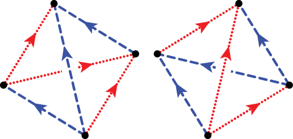
Figure 2.1. An ideal triangulation of the complement of the figure-eight knot in the three-sphere. Each edge is equipped with a colour -- red (dotted) or blue (dashed) -- and an orientation. These determine the face pairings. The flattening (into the plane) makes the triangulation taut and transverse. Note that the taut structure and the orientation determine the veering structure and thus the colours.

A model tetrahedron $t$ is taut if every model edge is equipped with a dihedral angle of zero or $\pi$, subject to the requirement that the sum of the three dihedral angles at any model vertex is $\pi$. It follows that there are exactly two model edges in $t$ with angle $\pi$; these do not share any vertex of $t$. The remaining four model edges, with angle zero, are called equatorial. A taut tetrahedron can be flattened into the plane with its equatorial edges forming its boundary; see Figure 2.1. A taut tetrahedron $t$ contains an equatorial square: a disk properly embedded in $t$ whose boundary is the four equatorial edges. An ideal triangulation $\mathcal{T}$ of $M$ is a taut triangulation if the model tetrahedra are taut and, for every edge $e$ in $|\mathcal{T}|$, the sum of the dihedral angles of the models of $e$ is $2\pi$ [13, Definition 1.1].

A taut model tetrahedron $t$ is transverse if every model face is equipped with a co-orientation (in or out of $t$), subject to the requirement that co-orientations agree across model edges of dihedral angle $\pi$ and disagree across model edges of dihedral angle zero. See Figure 2.2a. A taut triangulation $\mathcal{T}$ of $M$ is a transverse taut triangulation if every model tetrahedron is transverse taut and, for every face $f$ in $|\mathcal{T}|$, the associated face pairing preserves the co-orientations of the two model faces [13, Definition 1.2], [14, page 370].

2pt $0$ at 20 130 $0$ at 240 120 $0$ at 135 27 $0$ at 135 217 $\pi$ at 125 140 $\pi$ at 125 87

(a) Co-orientations and angles in a transverse taut tetrahedron.

(b) Co-orientations around edges can be deduced from the co-orientations on the faces of the model tetrahedra.

Figure 2.2.

Recall that the model tetrahedra are oriented. A taut model tetrahedron $t$ is veering if every model edge is equipped with a colour, red or blue, subject to the following.

• The colours on the equatorial edges alternate between red and blue.

• Viewing any model face (from the outside of the tetrahedron) the non-equatorial edge is followed, in anticlockwise order, by a red equatorial edge.

Suppose that $t$ is a veering tetrahedron. If the two non-equatorial edges of $t$ are both red (blue) then we call $t$ a red (blue) fan tetrahedron. If the two non-equatorial edges of $t$ have different colours then we call $t$ a toggle tetrahedron. See Figure 2.3a for all four of the possible veering model tetrahedra. Note that the taut structure and the orientation of $t$ determine the colouring of its equatorial edges.

Suppose now that $\mathcal{T}$ is a transverse taut triangulation of $M$. Then $\mathcal{T}$ is a transverse veering triangulation if there is a colouring of the edges of $|\mathcal{T}|$ making all of the model tetrahedra veering [1, Main construction], [13, Definition 1.3]. By the previous paragraph, when such a colouring exists it is unique. Also, if the colouring exists then the orientations of the model tetrahedra of $\mathcal{T}$ induce an orientation on $M$. For an example of a transverse veering triangulation, see Figure 2.1. The possible gluings between the various kinds of veering tetrahedra are recorded in Figure 2.3a.

(a) Upper tracks.

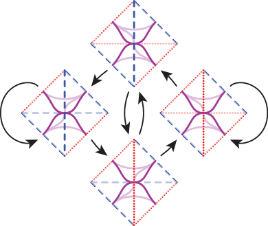
(b) Lower tracks.

Figure 2.3. In both subfigures, above and below we have toggle tetrahedra while left and right we have, respectively, blue and red fan tetrahedra. A black arrow indicates a possible gluing from an upper face of the initial tetrahedron to a lower face of the terminal. Note that fan tetrahedra of different colours never share a face. Finally, inside each tetrahedron $t$ on the left (right) we draw the branched surface $B^{t}$ ($B_{t}$).

2.2. Train-tracks

For background on train-tracks generally we refer to [17] as well as [21, Chapter 8]. Suppose that $\mathcal{V}$ is a transverse veering triangulation. Suppose that $f$ is a face of $\mathcal{V}$. Let $t$ and $t^{\prime}$ be the tetrahedra above and below $f$, respectively. We now define the upper and lower train-tracks $\tau^{f}$ and $\tau_{f}$ in $f$. The upper track $\tau^{f}$ consists of one switch at each edge midpoint and two branches perpendicular to the edges [1, Figure 11]. The two branches meet only at the switch on the non-equatorial edge of $t$ (the tetrahedron above $f$). The lower track $\tau_{f}$ is defined similarly, except the two branches now meet at the switch on the non-equatorial edge of $t^{\prime}$ (the tetrahedron below $f$). We call the region immediately between the two branches, adjacent to the shared switch, a track-cusp. See Figure 2.4. Starting in Section 7 we also discuss slightly more general train-tracks in slightly more general surfaces.

2pt $f$ at 88 71

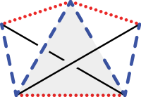
(a) The two taut tetrahedra adjacent to a face $f$ lie above and below $f$.

2pt $\tau^{f}$ [tr] at 65 42

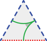
(b) The upper train-track $\tau^{f}$.

2pt $\tau_{f}$ [tl] at 77 37

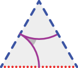
(c) The lower train-track $\tau_{f}$.

Figure 2.4.

2.3. Branched surfaces

For background on branched surfaces generally we refer to [5, Section 6.3].

Suppose that $M$ is an oriented three-manifold equipped with a transverse veering triangulation $\mathcal{V}$. Suppose that $t$ is a model tetrahedron of $\mathcal{V}$. The four faces $(f_{i})$ of $t$ contain their upper tracks $\tau^{i}$. These form a graph in $\partial t$, transverse to the edges of $t$. This graph bounds a normal quadrilateral and also a pair of normal triangles [12, page 4]. We arrange matters so that the three normal disks meet only along the lower faces of $t$, so that they are transverse to the equatorial square of $t$, and so that the union of the normal disks is a branched surface, denoted $B^{t}$. We call $B^{t}$ the upper branched surface in $t$. We define $B_{t}$, the lower branched surface in $t$ similarly, using the lower tracks $\tau_{i}$ instead of the upper. We finally define $B^{\mathcal{V}}=\cup_{t}B^{t}$ and $B_{\mathcal{V}}=\cup_{t}B_{t}$ to be the upper and lower branched surfaces for $\mathcal{V}$ in normal position. See Figure 2.5a.

We define the horizontal branched surface $B(\mathcal{V})$ to be the union of the faces of $\mathcal{V}$. Here we isotope the faces of $\mathcal{V}$, near their boundaries, to meet the one-skeleton of $\mathcal{V}$ as shown in Figure 2.2b. The horizontal branched surface $B(\mathcal{V})$ is taut [14, page 374]; this explains the name taut ideal triangulation.

The branch locus $\Sigma=\Sigma(B)$ of a branched surface $B$ is the subset of non-manifold points. Each component of $B-\Sigma$ is a sector of $B$. For $B^{\mathcal{V}}$ (and $B_{\mathcal{V}}$) a generic point of its branch locus is locally adjacent to exactly three sectors. The vertices of $B^{\mathcal{V}}$ (and $B_{\mathcal{V}}$) are the points of the branch locus locally meeting six sectors. Note that, since we have removed the zero-skeleton from $|\mathcal{V}|$, the horizontal branched surface $B(\mathcal{V})$ has no vertices [14, page 371].

We may move $B^{\mathcal{V}}$ into dual position by applying a small upward isotopy of $B^{\mathcal{V}}$. See Figure 2.5b. This done, every tetrahedron $t$ of $\mathcal{V}$ contains exactly one vertex of $B^{\mathcal{V}}$ and every face of $\mathcal{V}$ contains exactly one point of the branch locus. We arrange matters so that the vertex of $B^{\mathcal{V}}$ in $t$ is halfway between the lower edge and the equatorial square of $t$. Applying a small downward isotopy to $B_{\mathcal{V}}$ produces its dual position. We again arrange matters so that the vertex of $B_{\mathcal{V}}$ in $t$ is halfway between the upper edge (of $t$) and the equatorial square.

Remark 2.1.

In dual position, both $B^{\mathcal{V}}$ and $B_{\mathcal{V}}$ are isotopic to the dual two-skeleton of $\mathcal{V}$. See [10, Remark 6.4]. ∎

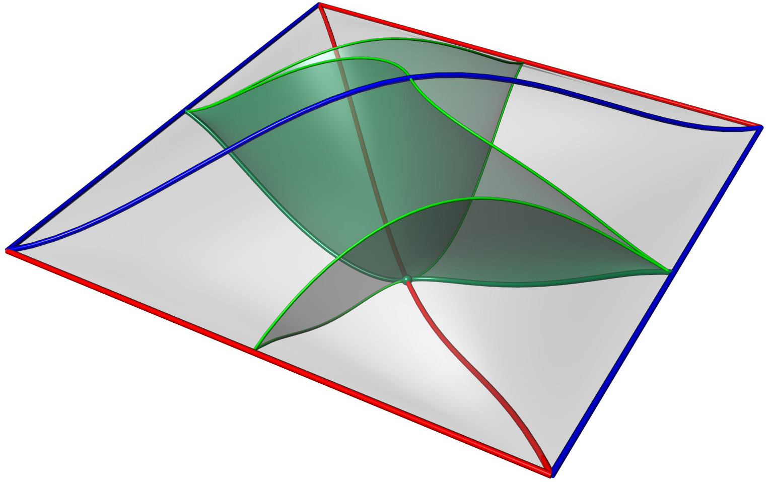
(a) Normal position.

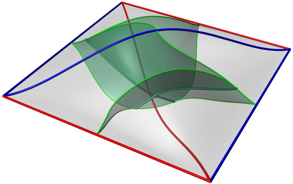
(b) Dual position.

Figure 2.5. Two positions of the upper branched surface in a tetrahedron.

Suppose that $M$ be an oriented three-manifold equipped with a transverse veering triangulation $\mathcal{V}$. Suppose that ${\widetilde{M}}$ is the universal cover of $M$. Suppose that ${\widetilde{B}}^{\mathcal{V}}$ and ${\widetilde{B}}_{\mathcal{V}}$ are the preimages of $B^{\mathcal{V}}$ and $B_{\mathcal{V}}$ in ${\widetilde{M}}$. We now restate [10, Corollary 6.12].

Lemma 2.2.

In the universal cover ${\widetilde{M}}$, with ${\widetilde{B}}^{\mathcal{V}}$ and ${\widetilde{B}}_{\mathcal{V}}$ in dual position, every subray of every branch line of ${\widetilde{B}}^{\mathcal{V}}$ and of ${\widetilde{B}}_{\mathcal{V}}$ meets toggle tetrahedra. ∎

3. Dynamics

Suppose that $M$ is a connected oriented three-manifold equipped with a riemannian metric. We loosely follow Mosher [16, page 36] for the next two definitions. See also [6, Figure 1.3].

Definition 3.1.

A dynamic vector field $X$ on $M$ is a smooth non-vanishing vector field. If $M$ has boundary then we require $X$ to be tangent to the boundary of $M$. ∎

The dynamic vector field $X$ gives us a local notion of upwards (the direction of $X$). Note that in our setting $X$ is smooth while in Mosher’s it is necessarily at best continuous.

Definition 3.2.

Suppose that $M$ is a three-manifold and $X$ is a dynamic vector field. Suppose that $B^{*}\subset M$ is a properly embedded branched surface. We say that $B^{*}$ is a stable dynamic branched surface with respect to $X$ if it has the following properties.

• For any point $p$ of any sector of $B^{*}$, there is a tangent to the sector, at $p$, which makes a positive dot product with $X$. Choosing the largest such gives a vector field $X^{*}$ on $B^{*}$. Integrating $X^{*}$ gives the upwards semi-flow.

• The semi-flow $X^{*}$ is transverse to the branch locus of $B^{*}$ and points from the side with fewer sheets to the side with more.

• The semi-flow $X^{*}$ is never orthogonal to the branch locus.

The only change needed to define an unstable dynamic branched surface $B_{*}$ is that $X_{*}$ points from the side with more sheets to the side with fewer. ∎

Note that Mosher requires his original vector field $X$ be tangent to $B^{*}$. However, we wish to use just one vector field with respect to which both branched surfaces $B^{\mathcal{V}}$ and $B_{\mathcal{V}}$ are dynamic (but do not yet form a dynamic pair).

Remark 3.3.

The terms stable and unstable come from the fact that any pseudo-Anosov flow $\Phi$ leads to a pair of two-dimensional foliations [5, page 226], [16, Section 3.1]. These are the weak stable foliation $F^{\Phi}$ and the weak unstable foliation $F_{\Phi}$. If $L$ is a leaf of $F^{\Phi}$ then any two flow lines $\ell$ and $\ell^{\prime}$ in $L$ are asymptotic in forward time. Finally, the stable branched surface $B^{\Phi}$ carries $F^{\Phi}$. ∎

Suppose that $t$ is one of the four model transverse veering tetrahedra (shown in Figure 2.3). Let $X_{t}$ be a non-vanishing vector field in $t$ with the following properties.

• The vector field $X_{t}$ is orthogonal to each face of $t$.

• Each orbit of $X_{t}$ connects a lower face of $t$ with an upper face.

• The branched surfaces $B^{t}$ and $B_{t}$ (in dual position) are stable and unstable with respect to $X_{t}$.

Now suppose that $\mathcal{V}$ is a transverse taut veering triangulation. We define $X_{\mathcal{V}}$ by gluing together the vector fields $X_{t}$.

Corollary 3.4.

The upper and lower branched surfaces $B^{\mathcal{V}}$ and $B_{\mathcal{V}}$ (in dual position) are, with respect to $X_{\mathcal{V}}$, stable and unstable dynamic branched surfaces. ∎

4. Dynamic pairs

In this section, loosely following Mosher [16, page 52], we give our definition of a dynamic pair of branched surfaces. Morally, these mimic the stable and unstable foliations of a pseudo-Anosov flow. The transversality of the foliations implies that the branched surfaces should be transverse and should not have various kinds of ‘‘bigon regions’’.

We make this precise and then discuss the main difficulties in proving Theorem 10.1.

4.1. Complementary components

Suppose that $M$ is a connected oriented three-manifold equipped with a riemannian metric. Suppose that $X$ is a dynamic vector field on $M$, as in Definition 3.1. Suppose that $B^{*}$ and $B_{*}$ are stable and unstable dynamic surfaces with respect to $X$. Suppose further that $B^{*}$ and $B_{*}$ meet transversely.

Definition 4.1.

Suppose that $C$ is a component of $M-(B^{*}\cup B_{*})$. We call $C$ a pinched tetrahedron if ${\overline{C}}$ (the closure taken in the induced path metric) has the following properties.

• ${\overline{C}}$ is a three-ball.

• $\partial{\overline{C}}$ consists of four triangles, called the faces of $C$.

• Each pair of faces meets in a simple arc; these six arcs form the one-skeleton of a tetrahedron.

• When mapped to $M$, two faces are sent to $B^{*}-B_{*}$ and two are sent to $B_{*}-B^{*}$.

• The two faces sent to $B^{*}-B_{*}$ meet in a single arc of (the preimage of) the branch locus of $B^{*}$; a similar property holds for the two faces sent to $B_{*}-B^{*}$. ∎

See Figure 4.1a for a picture of an embedded pinched tetrahedron.

(a) A pinched tetrahedron.

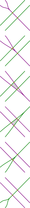
(b) Birth, life, and death.

Figure 4.1. The right shows horizontal slices through the left. See also Figures 2.2, 2.3 and 2.6 of [16].

Definition 4.2.

We call a foliation of (a three-dimensional region of) $M$ horizontal if it is everywhere transverse to $X$, to $B^{*}$, to $B_{*}$, and to $B^{*}\cap B_{*}$. ∎

The birth, life, and death of a pinched tetrahedron play out on the two-dimensional leaves of such a horizontal foliation.

Definition 4.3.

Suppose that $C$ is a pinched tetrahedron for $B^{*}$ and $B_{*}$. Since $C$ is simply connected for the purposes of this definition we may assume that $M$ is simply connected. Suppose that $(H_{s})_{s\in\mathbb{R}}$ is a horizontal foliation of a ball in $M$ containing $C$. As $s$ increases, we move upwards, in the direction of $X$. Let $\tau^{s}=H_{s}\cap B^{*}$ and $\tau_{s}=H_{s}\cap B_{*}$ be the upper and lower tracks in $H_{s}$ respectively. Let $C_{s}=C\cap H_{s}$. There are four special times $a<b<c<d$ as follows.

• At time $a$, the pinched tetrahedron $C$ is born as a track-cusp of $\tau^{a}$ crosses an arc of $\tau_{a}$, moving forwards.

• For $s\in(a,b)$, the disk $C_{s}$ is a green trigon. It has two sides and a track-cusp in $\tau^{s}$. The remaining side is in $\tau_{s}$.

• At time $b$, the track-cusp of $\tau^{b}$ (on the same branch line) crosses another arc of $\tau_{b}$, still moving forward.

• For $s\in(b,c)$, the disk $C_{s}$ is a quadragon. Its four sides alternate between $\tau^{s}$ and $\tau_{s}$.

• At time $c$, a track-cusp of $\tau_{c}$ crosses an arc of $\tau^{c}$, moving backwards.

• For $s\in(c,d)$, the disk $C_{s}$ is a purple trigon. It has two sides and a track-cusp in $\tau_{s}$. The remaining side is in $\tau^{s}$.

• At time $d$, the pinched tetrahedron $C$ dies as the track-cusp of $\tau_{d}$ (on the same branch line) crosses an arc of $\tau^{d}$, still moving backwards. ∎

Figure 4.1b shows $\tau^{s}\cup\tau_{s}$ for six representative generic heights.

Definition 4.4.

Suppose that $C$ is a component of $M-(B^{*}\cup B_{*})$. We call $C$ a dynamic torus shell if it is homeomorphic to $T^{2}\times(0,1)$. We require that for any $\epsilon$ the image of $T^{2}\times(0,\epsilon)$ in $C$ is an end of $M$. The other end of $C$ must have closure (in the path metric) homeomorphic to $T^{2}\times(1/2,1]$. The boundary of this must meet, in alternating fashion, annuli from $B^{*}-B_{*}$ and from $B_{*}-B^{*}$. The annuli from $B^{*}-B_{*}$ are the stable annuli of $C$ while the annuli from $B_{*}-B^{*}$ are the unstable annuli of $C$. See Figure 4.2.

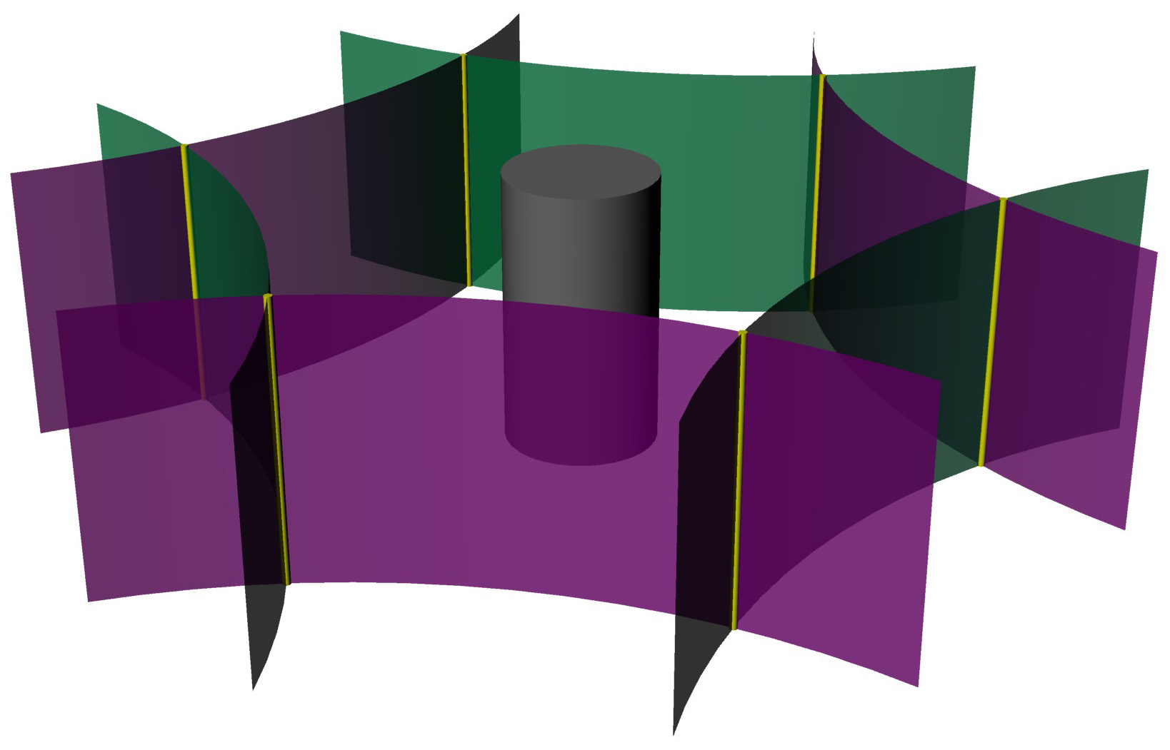
Figure 4.2. A section of an annulus or torus shell. The central grey cylinder represents an end of $M$.

Taking infinite degree covers of a dynamic torus shell yields (periodic) dynamic annulus shells and dynamic plane shells. More generally, such shells need not be periodic. This occurs only when neither $B^{*}$ nor $B_{*}$ is compact. There are two types of dynamic annulus shell. In one, the frontier is a bi-infinite alternating union of stable and unstable annuli. In the other, the frontier is a finite alternating union of stable and unstable strips of the form $[0,1]\times\mathbb{R}$. There is only one type of dynamic plane shell. Here the frontier is a bi-infinite alternating union of stable and unstable strips. Thus for any dynamic shell $C$, the components of the frontier (after cutting along $B^{*}\cap B_{*}$) are stable and unstable annuli or strips. These annuli or strips are the faces of the dynamic shell $C$. ∎

Definition 4.5.

Suppose that $C$ is a complementary region. Suppose that $F$ is an unstable face of ${\overline{C}}$. The components of $F-B^{(1)}_{*}$ are called the subfaces of $F$. The subfaces of a stable face are defined similarly. ∎

Definition 4.6.

A smooth path $\alpha$ in $B^{*}$ is upwards if it always crosses the branch locus of $B^{*}$ from the side with fewer sheets to the side with more. We make a similar definition for downwards paths in $B_{*}$. ∎

We are now equipped to give our definition of a dynamic pair.

Definition 4.7.

We say that $B^{*}$ and $B_{*}$ form a dynamic pair if they satisfy the following.

1. (Transversality): The branched surfaces $B^{*}$ and $B_{*}$ intersect transversely.

2. (Components): Every component of $M-(B^{*}\cup B_{*})$ is either a pinched tetrahedron or a dynamic shell.

3. (Transience): For every component $F$ of $B_{*}-B^{*}$ there is an unstable face $F^{\prime}\subset F$ of some dynamic shell so that $F^{\prime}$ is a sink for all upwards rays in $F$. The corresponding statement holds for downwards paths in $B^{*}-B_{*}$.

4. (Separation): No distinct pair of subfaces of dynamic shells are glued in $M$. ∎

Definition 4.8.

Suppose that $B^{*}$ and $B_{*}$ form a dynamic pair. Then their dynamic train-track is the intersection $B^{\mathcal{V}}\cap B_{\mathcal{V}}$. ∎

Remark 4.9.

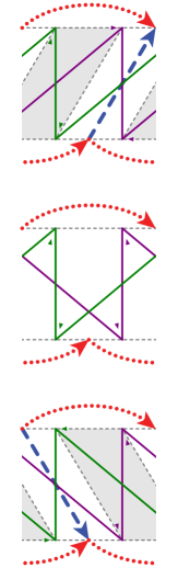
(a) Blue solid torus.

2pt c at 170 845 b at 170 780 a at 225 790 d at 225 735

c at 145 490 a at 70 500 a at 220 500 d at 245 425 d at 45 425 b at 110 415 b at 180 415

c at 120 195 b at 120 130 a at 65 140 d at 65 75

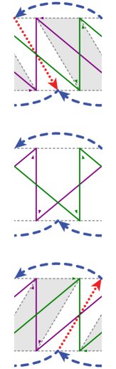
(b) Red solid torus.

Figure 9.10. Draped position for the figure-eight knot sibling with veering triangulation cPcbbbdxm_10 . The four pinched tetrahedra are labelled a through d. To obtain the pictures for the figure-eight knot complement with veering triangulation cPcbbbiht_12 , alter these figures by requiring that the orientation on every helical edge points upwards. (To relabel the pinched tetrahedra, start with those given at the top of Figure 9.10a and propagate outwards.)

Dynamic shells (and pinched tetrahedra) may meet each other or themselves along intervals of the dynamic train-track. For an example, see Figure 9.10. ∎

Our Definition 4.8 is taken directly from [16, page 54]. Note that our Definition 4.7 is more restrictive than Mosher’s [16, page 52]. Mosher allows dynamic shells to meet along subfaces while we do not. He also allows solid torus pieces. We do not require (or allow) solid torus pieces in the cusped case. In the closed case they are necessary; we deal with this as follows.

Remark 4.10.

Suppose that $\gamma$ is a curve in $T$, a torus boundary component of $M$. Suppose that $C$ is a dynamic torus shell containing $T$. Suppose that $\gamma$ meets the dynamic train-track (projected from $C$ to $T$) at least four times. Then Dehn filling $M$ along $\gamma$ converts $C$ into a solid torus piece $C(\gamma)$. So, after filling all dynamic torus shells we arrive at the closed case. ∎

4.2. The naive push-off

As noted in Remark 1.2, in normal position the branched surfaces $B^{\mathcal{V}}$ and $B_{\mathcal{V}}$ coincide in (at least) all normal quadrilaterals in all fan tetrahedra. To try and fix this, we choose orientations on the edges of $\mathcal{V}^{(1)}$. We then push $B_{\mathcal{V}}$ slightly in the directions of the edge orientations and pull $B^{\mathcal{V}}$ slightly against them. We call this pair of isotopies the naive push-off. In Examples 4.11 and 4.12 we see that this sometimes works and sometimes does not. The way in which the naive push-off fails is instructive; as noted in Remark 1.2 the obstructions are non-local.

Example 4.11.

In Figure 4.3a we draw an exploded view of the veering triangulation on the figure-eight knot complement, as previously introduced in Figure 2.1. The upper and lower train-tracks are the result of intersecting $B^{\mathcal{V}}$ and $B_{\mathcal{V}}$ with the faces and equatorial squares of the veering tetrahedra. The naive push-off keeps the dynamic branched surfaces dual to the horizontal branched surface $B=B(\mathcal{V})$ and makes them transverse to each other. Note that no pair of train-tracks in any horizontal cross-section form a bigon.

In fact, the push-off makes $B^{\mathcal{V}}$ and $B_{\mathcal{V}}$ into a dynamic pair. Parts (1) and (4) of Definition 4.7 can be checked cross-section by cross-section. For part (2), we have labelled cross-sections through the four pinched tetrahedra a_i through d_i, with subscripts indicating the vertical order. One must check that as we move vertically through the manifold, the sections through the regions assemble to form pinched tetrahedra (see Figure 4.1b) and dynamic torus shells. Note that in Figure 4.3a, as we move downwards from the middle section to the bottom of the two tetrahedra, regions c₁ and d₁ go from being quadragons to being green trigons (and then disappear), but the trigonal stage is not shown. Part (3) must be checked by hand. ∎

Example 4.12.

Consider the veering triangulation on the figure-eight knot sibling, shown in Figure 4.3b. Again we push $B_{\mathcal{V}}$ in the direction of the orientations of the edges; this time bigons appear in several of the horizontal cross-sections. In fact there is no orientation of the edges that leads to a dynamic pair via the naive push-off. This is because the mid-surface (Definition 5.14) for the figure-eight knot sibling is not transversely orientable. Further details are given in Remark 5.18. ∎

2pt b₄ at 104 407 a₆ at 51 402 d₂ at 104 384 a₂ at 83 373 b₄ at 48 358 a₆ at 103 354

b₃ at 104 254 a₅ at 67 238 b₇ at 112 230 d₁ at 103 213 b₃ at 48 201 a₅ at 103 197 a₁ at 85 184 c₃ at 70 184

b₂ at 99 104 a₄ at 52 100 b₆ at 82 87 b₂ at 48 48 a₄ at 99 42 c₂ at 70 30

a₄ at 205 407 b₆ at 257 402 c₂ at 205 384 b₂ at 227 373 a₄ at 261 358 b₆ at 206 354

a₃ at 205 254 b₅ at 242 238 a₇ at 201 230 c₁ at 208 213 a₃ at 261 201 b₅ at 206 197 b₁ at 224 183 d₃ at 239 186

a₂ at 210 104 b₄ at 257 100 a₆ at 227 87 a₂ at 261 48 b₄ at 210 42 d₂ at 239 32

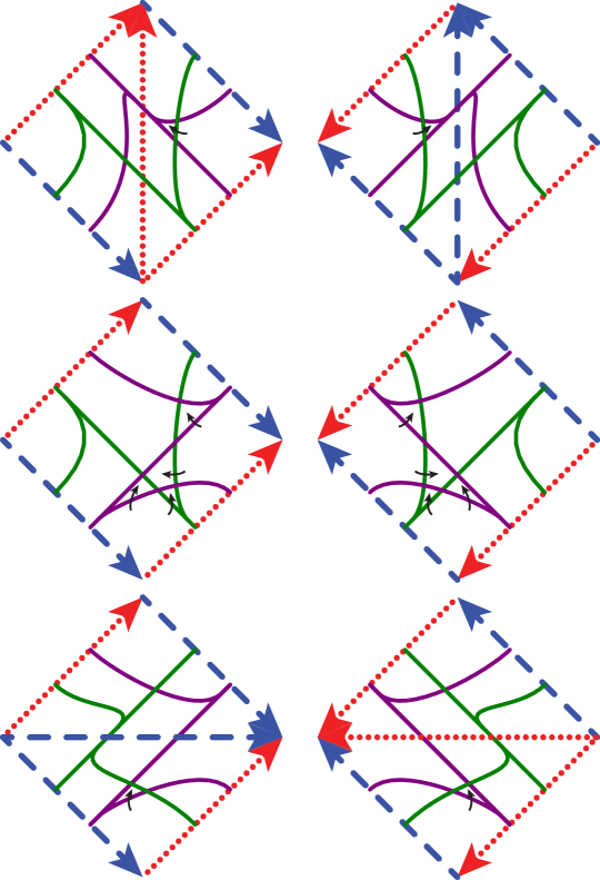
(a) The figure-eight knot complement with the veering triangulation cPcbbbiht_12 .

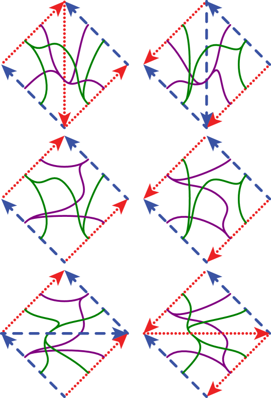
(b) The figure-eight knot sibling with the veering triangulation cPcbbbdxm_10 .

Figure 4.3. Canonical triangulations of the figure-eight knot complement and its sibling. Each column shows three slices: the upper and lower faces of, and an equatorial square through, one of the tetrahedra. In the figure-eight knot complement, $B^{\mathcal{V}}$ (green) and $B_{\mathcal{V}}$ (purple) have been naively pushed off each other to produce a dynamic pair. In the sibling, this does not work.

Even when it works, the naive push-off requires making a choice. Thus the resulting dynamic pair is not canonically associated to the initial veering triangulation.

Instead of isotoping the branched surfaces horizontally, we will ‘‘split’’ them closer to the stable and unstable foliations of the hypothesised pseudo-Anosov flow. To define these isotopies, we define various decompositions of $M$ (in Sections 5 and 6). We then describe a sequence of isotopies, of each of $B^{\mathcal{V}}$ and $B_{\mathcal{V}}$, through the new decompositions (in Sections 7, 8, and 9).

5. Shearing regions, mid-bands, and the mid-surface

Here we give a decomposition of a veering triangulation into a canonical collection of shearing regions. Each of these is either a solid torus or a solid cylinder. We use these to define the mid-bands and the mid-surface.

5.1. Shearing regions

Definition 5.1.

An ideal solid torus $U$ is a solid torus $D^{2}\times S^{1}$, together with a non-empty discrete subset of $(\partial D^{2})\times S^{1}$, called the ideal points of $U$. We define an ideal solid cylinder in similar fashion, replacing $S^{1}$ by $\mathbb{R}$. ∎

Definition 5.2.

A taut solid torus (cylinder) $U$ is an ideal solid torus (cylinder) decorated with a paring locus $\gamma$ containing all of the ideal points of $U$. The paring locus is a multi-curve $\gamma=\gamma(U)$ meeting every meridional disk exactly twice. There is at least one ideal point on every component of $\gamma$. A taut solid torus $U$ has a mid-band $B$; this is either an annulus or a Möbius band, properly embedded in $U$ and disjoint from $\gamma$. The mid-band of a taut solid cylinder is instead a strip, $[0,1]\times\mathbb{R}$. In all cases, the mid-band intersects every meridional disk in a single arc and every boundary compression of the mid-band intersects the pairing locus. ∎

Definition 5.3.

A transverse taut solid torus (cylinder) $U$ is a taut solid torus (cylinder) where $\partial U-\gamma$ has two components, called the upper and lower boundaries $\partial^{+}U$ and $\partial^{-}U$. These are equipped with transverse orientations that point out of and into $U$, respectively. Note that all taut solid cylinders can be equipped with such an orientation. ∎

In a transverse taut solid torus the mid-band is necessarily an annulus. In a taut solid cylinder it is necessarily a strip.

Definition 5.4.

A shearing region $U$ is a taut solid torus or cylinder, together with a colour (red or blue) and a squaring of $\partial U-\gamma$, with vertices at the ideal points. All edges contained in the paring locus $\gamma$ are the opposite colour to $U$ and are called longitudinal. All edges not in $\gamma$ are the same colour as $U$ and are called helical. The helical edges form a helix that spirals right or left (as $U$ is red or blue); the helix meets every meridional disk exactly once, transversely. We give the mid-band $B\subset U$ the same colour as $U$ itself. ∎

See Figure 5.1f for the local model of a red shearing region.

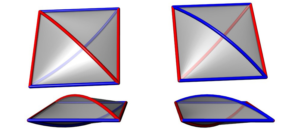
(a) Start with veering tetrahedra.

(b) Cut into half-tetrahedra, select red half-tetrahedra.

(c) Shear.

(d) Bend.

(e) Glue half-tetrahedra together.

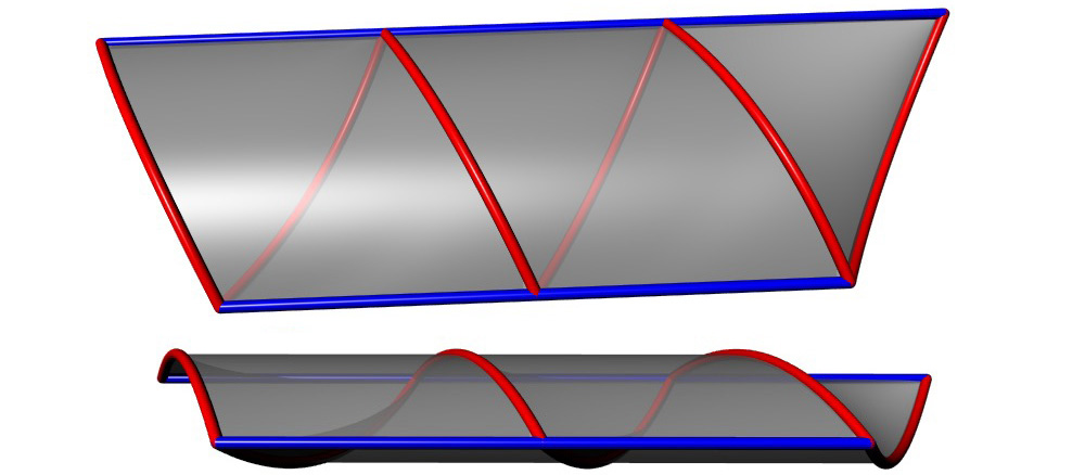
(f) Continue gluing.

Figure 5.1. Top and side views of the construction of a red shearing region.

Definition 5.5.

Suppose that $\mathcal{U}$ is a collection of model shearing regions. Let $\mathcal{U}^{(0)}$ be the set of ideal points. Suppose furthermore that the shearing regions are glued along all of their squares, respecting the colours of edges and so that every edge has exactly two helical models. We call $\mathcal{U}$ a shearing decomposition of $|\,\mathcal{U}-\mathcal{U}^{(0)}|$. The decomposition is called transverse if all of the shearing regions in $\mathcal{U}$ are transverse and the gluings respect the transverse orientations on the squares. ∎

Suppose that $\mathcal{V}$ is a veering triangulation (not necessarily transverse or finite). Recall from Section 2 that there are blue and red fan tetrahedra as well as toggle tetrahedra. Cutting a veering tetrahedron along its equatorial square results in a pair of half-tetrahedra; see Figure 5.1b. In every half-tetrahedra there is a unique (up to isotopy) half-diamond: this is a triangle, properly embedded in the half-tetrahedron, meeting only the edges of the colour of the $\pi$--edge, and those only exactly once at each midpoint. We give a half-diamond the colour of the edges it meets. See Figure 5.2. We arrange matters so that the two half-diamonds in a fan tetrahedron meet along their bases, and so form a full diamond. The two half-diamonds in a toggle tetrahedron $t$ meet in exactly one point: the centre of the equatorial square of $t$. For each half-diamond in a toggle tetrahedron, the central half of its intersection with the equatorial square is the boundary arc of the half-diamond. (In Definition 5.14, the union of the boundary arcs will give the boundary of the mid-surface.) Again, see Figure 5.2.

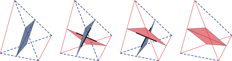
Figure 5.2. Diamonds and half-diamonds. Each half-diamond in a toggle tetrahedron has a boundary arc, shown here in black.

(a)

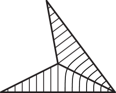
(b)

Figure 5.3. In Figure 5.3a we see adjacent half-diamonds in a veering triangulation. In Figure 5.3b we see an unpleasant possibility for adjacent half-diamonds in a taut triangulation.

Theorem 5.6.

Suppose that $\mathcal{V}$ is a veering triangulation (not necessarily transverse or finite). Then there is a canonical shearing decomposition of $M$ associated to $\mathcal{V}$.

Proof.

Suppose that $t$ is a half-tetrahedron and $d$ is its half-diamond. Fix a vertical line field on $d$ as shown in the left-most half-diamond of Figure 5.3a. Let $f$ and $f^{\prime}$ be the triangular faces of $t$. The colour of $d$ is the majority colour of the edges of $t$. Thus the colour of $t$ and $d$ matches the majority colour of both $f$ and $f^{\prime}$. Suppose that $t$ is glued to another half-tetrahedron, $t^{\prime}$, across $f^{\prime}$. Let $d^{\prime}$ be the half-diamond of $t^{\prime}$. Thus $d^{\prime}$ and $d$ have the same colour.

Note that the $\pi$–edges of $t$ and $t^{\prime}$ are distinct edges of the model face $f^{\prime}$. (This follows from the definition of a veering triangulation: see Figure 2.4a.) Thus, as shown in Figure 5.3a, we can locally extend the vertical line field on $d$, through $f^{\prime}$, to $d^{\prime}$. See Figure 5.1e. Let $f^{\prime\prime}$ be the other triangular face of $t^{\prime}$. Continuing in this fashion in both directions, we obtain a shearing region. The union of the half-diamonds is the mid-band. See Figure 5.4. ∎

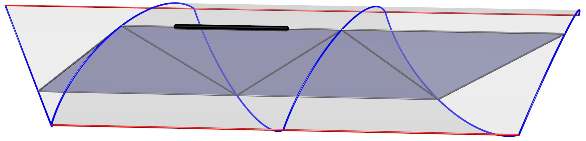
(a) Three-quarters view.

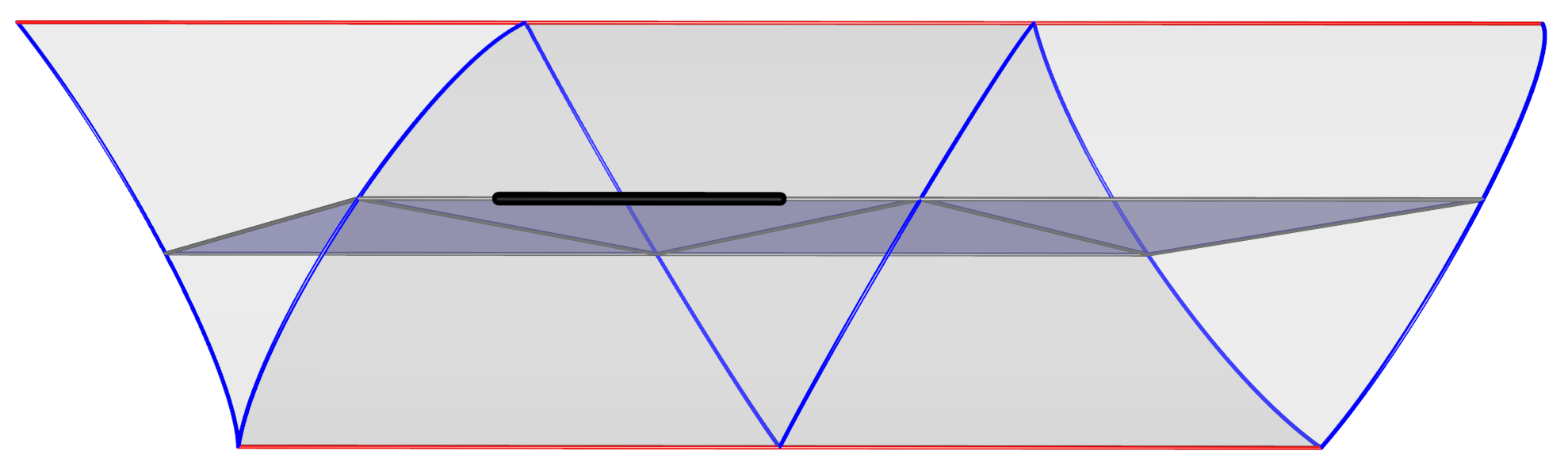
(b) View from above.

Figure 5.4. A red shearing region, with embedded mid-band. The boundary arc of the half-diamond (contained in a half-tetrahedron contained in a toggle tetrahedron) is drawn in black.

We give examples of mid-bands in Figures 5.5, 5.6, 5.7, and 5.8. These are taken from the veering census [11]. For each example we draw, in one column per tetrahedron, its upper and lower faces. On the faces we indicate their intersections with $B^{\mathcal{V}}$ and $B^{\mathcal{V}}$ after the straightening isotopy. We also draw the mid-annuli. See Figures 7.1, 7.2, and 7.3.

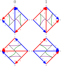
(a) Tetrahedra.

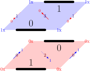
(b) Mid-annuli.

Figure 5.5. A veering triangulation for m004 from the SnapPea census [8]. This is cPcbbbiht_12 in the census of transverse veering triangulations [11].

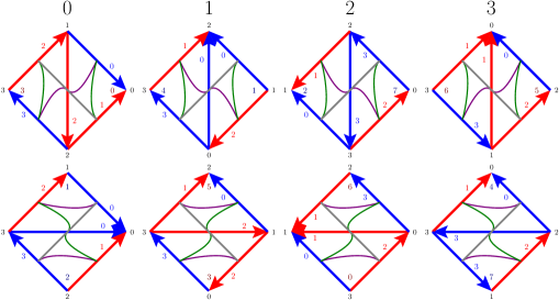
(a) Tetrahedra.

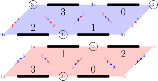
(b) Mid-annuli.

Figure 5.6. m203 , eLMkbcddddedde_2100 .

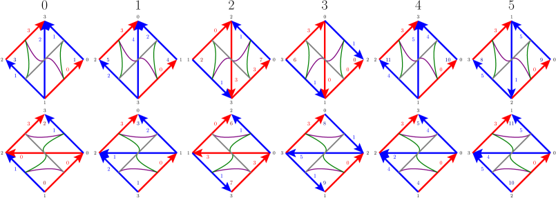
(a) Tetrahedra.

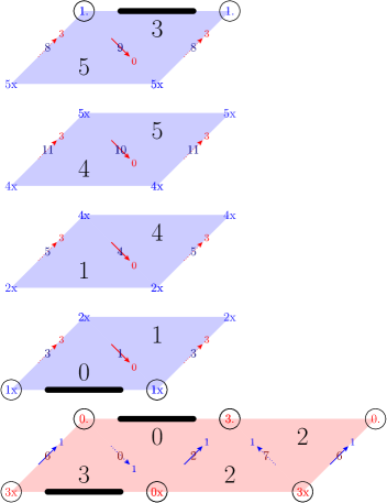
(b) Mid-annuli.

Figure 5.7. s227 , gLLAQbecdfffhhnkqnc_120012 .

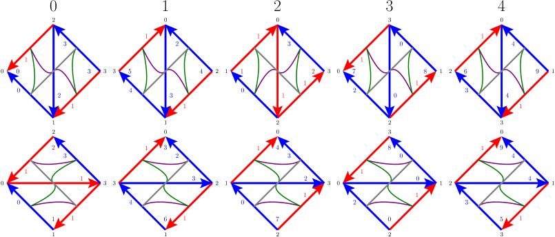
(a) Tetrahedra.

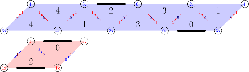
(b) Mid-annuli

Figure 5.8. m115 , fLLQccecddehqrwjj_20102 .

Remark 5.7.

If the veering triangulation $\mathcal{V}$ is transverse then the half-tetrahedra in each shearing region alternate between being the upper and lower halves of tetrahedra. Thus the transverse structure on $\mathcal{V}$ induces a transverse structure on the associated shearing decomposition. ∎

Remark 5.8.

Suppose that $\mathcal{V}$ is a finite transverse veering triangulation. We may interpret each shearing solid torus as a fractional Dehn twist. Thus the shearing decomposition (canonically) factors the “upwards dynamical system” as a product of fractional Dehn twists.

Despite this (and despite Corollary 1.1) it is not the case that every pseudo-Anosov homeomorphism decomposes as a product of fractional Dehn twists. ∎

Question 5.9.

Let $\gamma(U)$ be a core curve for the shearing region $U$. Performing certain Dehn fillings along $\gamma(U)$ produces new veering triangulations; see [18] and [23, Definition 4.1]. Let $\gamma(\mathcal{V})$ be the union of the curves $\gamma(U)$.

Suppose that $U$ and $V$ are a pair of regions. Suppose that the upper boundary of $U$ equals the lower boundary of $V$. That is, suppose that $\partial^{+}U=\partial^{-}V$. Then $\gamma(V)$ is parallel to $\gamma(U)$; accordingly we delete $\gamma(V)$ from $\gamma(\mathcal{V})$.

Now $\gamma(\mathcal{V})$ is a link canonically associated to $M$ and $\mathcal{V}$. What are the geometric properties of $M-\gamma(\mathcal{V})$? ∎

5.2. Crimping

Here we define the crimped shearing decomposition of $M$. This ensures that the union of the shearing regions of a fixed colour is a manifold (with various inward and outward paring loci) containing all of the veering edges of that colour. Crimping also improves the way that the mid-bands meet. Their union becomes the mid-surface. Crimping is similar to folding, in a train-track, all switches with both in- and out-degree bigger than one.

Suppose that $\mathcal{V}$ is a veering triangulation. The associated crimped shearing decomposition is obtained as follows.

Definition 5.10.

The equatorial branched surface $E(\mathcal{V})$ is the union of the equatorial squares of all veering tetrahedra. ∎

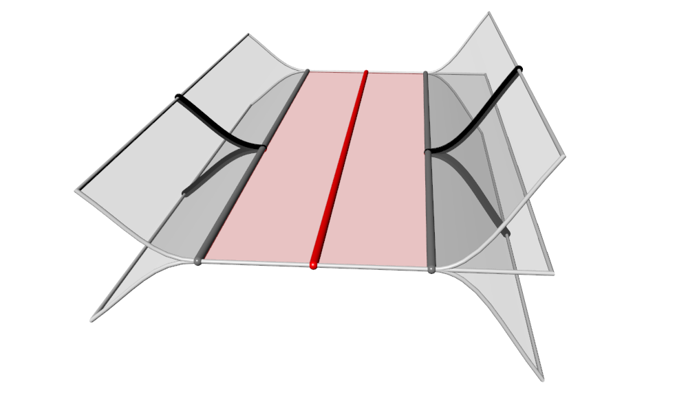
Figure 5.9. Top row: An edge $e\in\mathcal{V}^{(1)}$ before and after crimping on the right. No crimping is required on the left. Bottom row: Both sides are crimped. The veering edges are drawn in red, the crimped edges are drawn in grey, and the boundary arcs are drawn in black. The neighbourhoods $N_{\prec}(e)$ and $N_{\succ}(e)$, and the crimped rectangles, are shaded red.

Note that an edge $e\in\mathcal{V}^{(1)}$ lies in the branch locus of $E(\mathcal{V})$ if and only if the degree of $e$ (in $E(\mathcal{V})$) is at least three. Suppose that there are at least two squares to the right of $e$. Let $N_{\prec}(e)$ be a collar neighbourhood to the right side of $e$, taken inside of $E(\mathcal{V})$. (We choose the size of the collar neighbourhood so that it meets each boundary arc of each adjacent half-diamond in a single point.)

So $N_{\prec}(e)$ contains $e$ and a rectangle for every equatorial square to its right. See Figure 5.9 (upper left) for a picture of one possible $N_{\prec}(e)$. We define $N_{\succ}(e)$ similarly, again when there are at least two squares to the left of $e$. See Figure 5.9 (lower left).

Definition 5.11.

We obtain the crimped equatorial branched surface $E_{\succ\!\prec}(\mathcal{V})$ from the equatorial branched surface $E(\mathcal{V})$ by crimping edges, as follows. For every veering edge $e$, fold together all rectangles in $N_{\prec}(e)$ to obtain a single rectangle; do the same to the left collar $N_{\succ}(e)$. ∎

After crimping the sides of all veering edges (having at least two squares), the veering edges are disjoint from the branch locus of $E_{\succ\!\prec}(\mathcal{V})$. Also, there are no vertices in $E_{\succ\!\prec}(\mathcal{V})$. Thus we call the components of $E_{\succ\!\prec}^{(1)}(\mathcal{V})$ crimped edges. The midpoint of each crimped edge equals the endpoints of two boundary arcs. See Figure 5.9 (right) for pictures of possibilities for $E_{\succ\!\prec}(\mathcal{V})$.

Suppose that we had to crimp the right side of $e$. So, before crimping, $N_{\prec}(e)$ contained two or more rectangles. Then, after crimping, there is a single crimped rectangle between $e$ and the crimped edge immediately to the right of $e$. Note that two closed crimped rectangles are either disjoint or meet along their common veering edge. In our figures we colour the crimped edges as a dashed grey. Since we draw pictures in the cusped manifold, we will refer to the crimped rectangle as a crimped bigon. In Figures 5.9, 5.11, and 7.1 through 7.4 we shade crimped bigons the colour of their veering edge.

Crimping moves the equatorial square of a toggle tetrahedron into $E_{\succ\!\prec}(\mathcal{V})$. There it is subdivided, by the crimped edges, into four crimped bigons and one toggle square. In our figures we shade the toggle squares in grey. Since crimped bigons are disjoint, every toggle square has four cusps that reach out to the ideal points of the three-manifold. See Figure 5.10a. (The widths of these cusps are set in Section 8.3.)

The two boundary arcs (of the mid-surface) in the toggle tetrahedron lie inside of the toggle square. They end at the midpoints of the crimped edges and divide the toggle square into four symmetric regions. See Figure 5.10a. The veering hypothesis implies that a crimped bigon meets, along its crimped edge, exactly two toggle squares: one at the top and one at the bottom of a stack of fan tetrahedra. Similarly, the equatorial square of a fan tetrahedron is subdivided into two crimped bigons and one fan square. See Figure 5.10b.

Definition 5.12.

For every cusp $c$ of every toggle square $S$ we choose a short arc $\alpha_{c}$ properly embedded in $S$ which separates the cusp $c$ from the body of $S$. The arc $\alpha_{c}$ meets exactly two crimped edges on the boundary of $S$.

Suppose that $e$ is a crimped edge on the boundary of $S$. Note that $e$ is adjacent to exactly two toggle squares: $S$ is one and suppose that $S^{\prime}$ is the other. Let $\alpha^{\prime}_{c}$ be the chosen short arc cutting the cusp $c$ off of $S^{\prime}$. We arrange matters so that the end points of $\alpha_{c}$ and $\alpha^{\prime}_{c}$ on $e$ coincide.

Thus the union of all of the chosen arcs gives an embedded collection of loops and lines in the three-manifold; the components of the union are isotopic into the ideal points of the three-manifold. We take a small tubular neighbourhood of this union. (The radius of the tubular neighbourhood varies; the details are given in Section 8.3.) We call a connected component of the result a station.

Suppose that $\Sigma$ is a station. Suppose that $S$ is a toggle square meeting $\Sigma$. Let $E$ be the equatorial square containing $S$. Looking from above, the cusp of $S$ meeting $\Sigma$ lies between two veering edges of $E$, one red and one blue. If these are ordered red then blue as we walk anticlockwise around $\partial E$ then we say that $\Sigma$ is an upper station. Otherwise $\Sigma$ is a lower station. ∎

The naming scheme for stations is explained in Section 8. There upper track-cusps will pass through upper stations, and similarly for lower track-cusps and lower stations.

In Figure 5.10, the intersection of the stations with the squares is shown with dots coloured green (for upper stations) or purple (for lower stations).

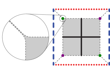
(a) Toggle square.

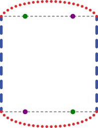
(b) Fan square.

Figure 5.10. The toggle square has four adjacent crimped bigons, the fan square has two. Here we draw the boundary arcs (of the half-diamonds immediately above and below) on the toggle square in black. The crimped edges are drawn in dashed grey. The upper and lower stations are here represented as small green and purple disks following the convention given in Definition 5.12.

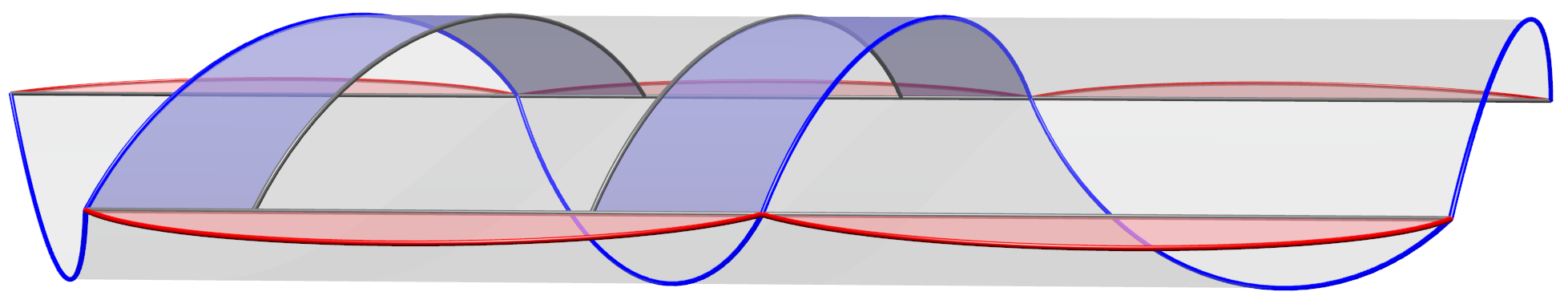
(a) View from the side.

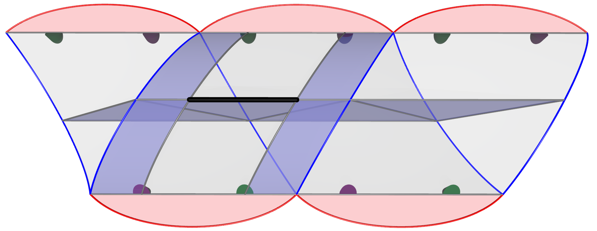
(b) View from above, with the mid-band and station (after intersecting with the crimped shearing region).

Figure 5.11. A crimped blue solid torus, and incident red crimped bigons. The crimped edges are drawn in grey and meet the boundary arc in its endpoints. Wherever the red and blue crimped bigons appear to meet, they are in fact separated by a cusp of the adjacent toggle square. See Figure 5.10a.

We define the (closures taken in the path metric of) components of $M-E_{\succ\!\prec}(\mathcal{V})$ as crimped shearing regions. See Figure 5.11. Let $U$ be a model crimped shearing region. As before, we write $\partial^{+}U$ and $\partial^{-}U$ for the upper and lower boundaries of $U$. Suppose that $e$ and $e^{\prime}$ bound a crimped bigon $B$ with $e\in\mathcal{V}^{(1)}$ and $e^{\prime}$ a crimped edge. If $B$ lies in either $\partial^{+}U$ or $\partial^{-}U$ then we say that $e$ and $e^{\prime}$ are helical for $U$. If $B\cap U=e^{\prime}$ then we say that $e$ and $e^{\prime}$ are longitudinal for $U$. Note that $\partial^{+}U\cap\partial^{-}U$ is the collection of longitudinal crimped edges for $U$.

Note that the stations meet $U$ in a collection of three-balls. Each such three-ball meets $\partial U$ in a disk. This disk is cut into exactly two pieces by the longitudinal crimped edge which it meets.

As before, we assign $U$ the colour of its helical edges. This colour is opposite to that of each edge of $\mathcal{V}^{(1)}$ that is parallel, across a crimped bigon, to the longitudinal crimped edges of $U$.

Within $U$, we replace each triangle of the original triangulation with a corresponding crimped triangle. The sides of each crimped triangle consist of two helical edges, one on $\partial^{+}U$ and one on $\partial^{-}U$, and a single longitudinal crimped edge.

The union of the crimped shearing regions is again homeomorphic to $M$; together they form the crimped shearing decomposition of $M$.

Definition 5.13.

The union of the red crimped shearing regions is the red submanifold of the crimped shearing decomposition. A connected component of the red submanifold is a red component. We define the blue submanifold and blue components similarly. These form the components of the monochromatic decomposition. ∎

Each red component is a handlebody with inward and outward paring loci. The red submanifold of the monochromatic decomposition contains all of the red edges of $\mathcal{V}^{(1)}$. Furthermore, its material boundary is the union of the toggle squares. Analogous statements are true for blue components and the blue submanifold.

5.3. The mid-surface

The mid-bands sit within the crimped shearing regions just as they sat within the original shearing regions. See Figure 5.11b. We may now glue the mid-bands to each other along their boundaries obtain a surface.

Definition 5.14.

The union of the red mid-bands in the red submanifold gives the red mid-surface $\mathcal{S}_{R}$. We build the blue mid-surface $\mathcal{S}_{B}$ in a similar fashion. We define the mid-surface to be $\mathcal{S}=\mathcal{S}_{R}\cup\mathcal{S}_{B}$. ∎

Note that each component of $\mathcal{S}_{R}$ sits inside, and is a deformation retract of, a red component of the crimped shearing decomposition. Thus $\mathcal{S}_{R}$ meets all red edges but no blue edges. A similar statement holds for $\mathcal{S}_{B}$. Each boundary arc of $\mathcal{S}_{R}$ meets precisely one boundary arc of $\mathcal{S}_{B}$; these intersect in a single point at the centre of the corresponding toggle square.

Note that $\mathcal{S}_{R}$ and $\mathcal{S}_{B}$ receive cell-structures from the (images under crimping of the) half-diamonds. Taking a horizontal union of half-diamonds yields a mid-band. Taking a diagonal union of half-diamonds (stopping at toggle squares, if any) yields a diagonal strip. Lemma 2.2 implies the following.

Corollary 5.15.

Every diagonal strip starts and ends at toggle squares. Thus every component of $\mathcal{S}_{R}$ and of $\mathcal{S}_{B}$ has at least one boundary component. ∎

Example 5.16.

In Figure 5.8 the red mid-surface has two diagonal paths, both traversing two half-diamonds. The blue mid-surface also has two diagonal paths, one traversing six half-diamonds and the other traversing ten. ∎

Every boundary component of the mid-surface runs alternatingly along boundary arcs contained in the upper and lower boundaries of crimped shearing regions. In Figures 5.5b, 5.6b, 5.7b, and 5.8b we give several examples; the boundary arcs are indicated by thick black lines. In Figure 5.5b both mid-surfaces are once-holed tori; each boundary component of each mid-surface consists of two boundary arcs. In Figure 5.6b both mid-surfaces are copies of $N_{3,1}$: the non-orientable surface with one boundary component and three cross-caps. In Figure 5.7b both mid-surfaces are copies of $N_{2,1}$: the once-holed Klein bottle. (This last was the first example of a non-fibered veering triangulation; see [13, Section 4].) Finally, in Figure 5.8b the mid-surfaces are a pair of once-holed Klein bottles, with one having greater area than the other.

Remark 5.17.

Mid-surfaces also allow one to see the walls of a veering decomposition, as defined by Agol and Tsang [2, Definition 3.3]. For example, in Figure 5.8 there is a wall of width three consisting of the tetrahedra 4 and 1. ∎

5.4. Labelling the mid-surface

We now describe the labelling scheme for the mid-surfaces used in the census [11]. This is useful when drawing pictures and discussing examples. Suppose that $\mathcal{V}$ is a finite transverse veering triangulation. We number the tetrahedra, the faces, the edges, and the vertices of the tetrahedra using the conventions from Regina [3]. Regina also provides us with orientations for the edges of $\mathcal{V}^{(1)}$; we will alter these to make them agree, as much as possible, with transverse orientations of mid-annuli.

We give four examples in Figures 5.5, 5.6, 5.7, and 5.8. For each example, we draw its mid-annuli and, in one column per tetrahedron, the upper and lower faces for each tetrahedron (viewed from above). On each face we draw the upper (green) and lower (purple) train-tracks. (Where these intersect, the intersection is coloured grey.)

In order to draw a mid-band $A=A(U)$ we choose a transverse orientation for it; this then induces a transverse orientation on each half-diamond $d$ of $A$.

In the examples of Figures 5.5, 5.6, 5.7, and 5.8 the mid-bands are all annuli and the transverse orientation points into the page.

We label the vertices, edges, and face of the half-diamond $d$ as follows.

• Suppose that $v$ is a vertex of $d$. We label $v$ with the number of the edge $e$ in $\mathcal{V}^{(1)}$ which contains $v$. Note that $e$ is helical for $U$. We append this number with one of the symbols from $\{\cdot,\text{x}\}$. The x means that the orientation of $e$ agrees with the transverse orientation on $d$; the dot means the opposite. (The x represents the fletching of an arrow, while the dot represents the arrowhead.)

• Suppose that $\epsilon$ is a diagonal edge of $d$. We label $\epsilon$ with the number of the face $f$ in $\mathcal{V}^{(2)}$ which contains $\epsilon$; we place the label at the midpoint of $\epsilon$. The vertices of $\epsilon$ are already labelled with the numbers of two of the three edges of $f$. Let $e$ be the third edge of $f$. Note that $e$ is longitudinal for $U$. We draw a small copy of $e$ on top of $\epsilon$ and label the copy with the number of $e$ (in the other colour and using a smaller font). Note that $\epsilon$ and $e$ cobound a rectangle in $f$; we use this rectangle to transport the orientation of $e$ to $\epsilon$. Finally, we draw the arrow dotted or solid as the transverse orientation on $d$ points towards or away from $e$. (That is, as drawn in Figures 5.5, 5.6, 5.7, and 5.8, the edge $e$ is behind or in front of $A$.)

• Suppose that $\epsilon$ is the base of a half-diamond $d$. If $d$ lies in a toggle tetrahedron then we draw a thick black line on $\epsilon$, to indicate the boundary arc on $d$.

• Finally, we label $d$ itself with the number of the tetrahedron that contains $d$.

Suppose that $A$ and $B$ are mid-annuli. Let $\partial^{-}A$ be the lower boundary of $A$, minus the open boundary arcs. Thus $\partial^{-}A$ is either a single line, a single circle, or a collection of intervals and at most two rays. We define $\partial^{+}B$ similarly. Suppose that $A$ and $B$ are glued to each other, say with a component $\gamma$ of $\partial^{-}A$ meeting a component of $\partial^{+}B$. (It is also possible for $A$, say, to be glued to itself.) We call the gluing $\gamma$ untwisted or twisted exactly as it does or does not faithfully transport the chosen transverse orientation on $A$ to the one on $B$.

In Figures 5.5, 5.6, 5.7, and 5.8 we indicate a twisted gluing by drawing a small black circle about all vertices of the affected boundary circle or sub-arc. We have chosen the transverse orientations of the mid-annuli to minimise the number of half-twists required.

Remark 5.18.

If all gluings are untwisted then the mid-surface is transversely orientable and thus orientable. Conversely, if the mid-surface is orientable then there is a choice of transverse orientations for the mid-bands that ensures that all gluings are untwisted. The naive push-off discussed in Section 4.2 should produce a dynamic pair when and only when the mid-surface is orientable.

Thus, if one is willing to pass to a double cover, then there should be edge orientations making the naive push-off work. However this push-off will not be invariant under the deck transformation. ∎

6. Bigon coordinates

In this section we place a coordinate system on the crimped shearing regions (introduced in Section 5.2). We also give a refinement of the crimped shearing decomposition of $M$ and introduce the horizontal cross-sections.

Let $B$ be a coordinate bigon: a oriented disk with two marked points $x$ and $y$ in its boundary. The points $x$ and $y$ are the corners of $B$. We equip $\partial B$ with the induced orientation. The two arcs of $\partial B-\{x,y\}$ are denoted by $\partial^{+}B$ and $\partial^{-}B$ respectively. We arrange matters so that $\partial^{+}B$ is the arc running from $y$ to $x$.

We equip $B$ with a pair of transverse foliations: the horizontal arcs all meet both corners while the vertical arcs all meet $\partial^{+}B$ and $\partial^{-}B$. We orient the former from $x$ to $y$ and the latter from $\partial^{-}B$ to $\partial^{+}B$. See Figure 6.1a.

We subdivide $B$ into a pair of sub-bigons called $\theta^{B}$ (upper) and $\theta_{B}$ (lower). These are shown in Figure 6.1b.

2pt $x$ [r] at 0 175 $y$ [l] at 575 175 $\partial^{+}B$ [br] at 120 300 $\partial^{-}B$ [tr] at 120 50

(a) Model bi-foliated coordinate bigon.

2pt $\theta^{B}$ at 290 250 $\theta_{B}$ at 290 100

(b) Bigon regions.

Figure 6.1.

Recall that $M$ is oriented and $\mathcal{V}$ is transverse veering. Suppose that $U$ is a model crimped shearing region. Thus $U$ inherits an orientation and, by Remark 5.7, a notion of ‘‘upwards’’. We now choose a homeomorphism $h$ between $U$ and $B\times S^{1}$ or $B\times\mathbb{R}$, as $U$ is a solid torus or cylinder. We require that $h$ preserve the various orientations. In particular, the upper boundary of $B$ is sent to the upper boundary of $U$ by $h$. We call $h$ the bigon coordinates for $U$.

Let $\Theta^{U}$ be the image of $\theta^{B}\times S^{1}$ (or $\theta^{B}\times\mathbb{R}$) in $U$. We define $\Theta_{U}$ similarly. Note that the upper boundaries of $U$ and $\Theta^{U}$ agree, as do the lower boundaries of $U$ and $\Theta_{U}$. That is, $\partial^{+}U=\partial^{+}\Theta^{U}$ and $\partial^{-}U=\partial^{-}\Theta_{U}$. Also, we have $\partial^{-}\Theta^{U}=\partial^{+}\Theta_{U}$. We take $\Theta^{\mathcal{V}}\subset M$ to be the union of the $\Theta^{U}$, taken over all model crimped shearing regions and then projected to $M$. We define $\Theta_{\mathcal{V}}$ similarly. The interiors of $\Theta^{\mathcal{V}}$ and $\Theta_{\mathcal{V}}$ are disjoint and their union is $M$; this is the $\Theta$--decomposition.

Remark 6.1.

Suppose that $U$ is a blue shearing region. We arrange the metric in $U$ (coming from bigon coordinates) to ensure the following.

1. In the induced coordinates on $\partial^{+}U$ the (pullbacks of the) blue edges of $\mathcal{V}^{(1)}$ are straight and, when viewed from above, have slope $\sqrt{3}$. Similarly, the blue edges in $\partial^{-}U$ are straight and, when viewed from above, have slope $-\sqrt{3}$.

2. For $p\in U$ we take $B(p,U)$ to be the coordinate bigon in $U$ containing $p$. Then the two notions of vertical (coming from the coordinate bigons $B(p,U)$ and the transverse veering structure) agree. Furthermore, the intersection of the mid-band $A(U)$ with any $B(p,U)$ is the central vertical arc of the latter.

3. As noted in Definition 5.12, each longitudinal crimped edge intersects the stations in two short intervals. These intervals appear slightly more than one-quarter of the length of the edge in from the ideal points of the three-manifold.

See Figure 5.11. We similarly give bigon coordinates to red model crimped shearing regions. ∎

We use the following notations for the various coordinate arcs and surfaces in bigon coordinates.

Definition 6.2.

Suppose that $U$ is a model crimped shearing region. Fix $p\in U$.

• As above, $B(p,U)$ is the coordinate bigon containing $p$.

• Let $x(p,U)=p\times S^{1}$ ($p\times\mathbb{R}$) be the horizontal circle (line) in $U$ through $p$.

• Let $y(p,U)$ be the leaf of the horizontal foliation of $B(p,U)$, through $p$.

• Let $z(p,U)$ be the leaf of the vertical foliation of $B(p,U)$, through $p$.

• Let $Y(p,U)$ be the union of the leaves $z(q,U)$ as $q$ ranges over $x(p,U)$. We call $Y(p,U)$ the vertical band in $U$ through $p$.

• Let $Z(p,U)$ be the union of the leaves $x(q,U)$ as $q$ ranges over $y(p,U)$. We call $Z(p,U)$ the (horizontal) cross-section in $U$ through $p$.

• Finally, we define $X(p,U)=B(p,U)$. ∎

Note that the upper and lower boundaries of $\Theta^{U}$ and $\Theta_{U}$ are horizontal cross-sections.

7. Straightening and shrinking

From now on, instead of working in $M$, we work in the universal cover ${\widetilde{M}}$. Thus we take care to ensure that our constructions are invariant under the action of the deck group. In a slight abuse of notation we continue to write $B^{\mathcal{V}}$ instead of the more correct ${\widetilde{B}}^{\mathcal{V}}$.

Here we define the straightening and shrinking isotopies. These are applied to the upper and lower branched surfaces $B^{\mathcal{V}}$ and $B_{\mathcal{V}}$. The isotopies are local: in each tetrahedron they (and the resulting shrunken position) depend only on the combinatorics of that tetrahedron and its immediate neighbours.

The branched surfaces begin in dual position (shown in Figure 2.5b). We straighten the branched surfaces to move as much of each as possible into the mid-surface $\mathcal{S}=\mathcal{S}_{R}\cup\mathcal{S}_{B}$. We shrink the branched surfaces to move vertices of $B^{\mathcal{V}}$ down into $\Theta_{\mathcal{V}}$ and those of $B_{\mathcal{V}}$ up into $\Theta^{\mathcal{V}}$.

We now describe in detail the upper straightening and shrinking isotopies of $B^{\mathcal{V}}$. The corresponding isotopies of $B_{\mathcal{V}}$ are defined similarly.

7.1. Straightening

First we straighten. We start with $B^{t}$ in dual position (shown in Figure 2.5b) and note that we have crimped. For a half-tetrahedron $h$ we take the sectors of $B^{h}$ that do not intersect any longitudinal crimped edge; we move those sectors to coincide with the (images after crimping of the) half-diamond of $h$.

The resulting position of the upper branched surface, in the various crimped half-tetrahedra, is shown in Figures 7.1, 7.2, and 7.3. Each figure has a $180^{\circ}$ symmetry about its central vertical axis. The resulting position of $B^{\mathcal{V}}$, in a piece of a crimped shearing region, is shown in Figure 7.4.

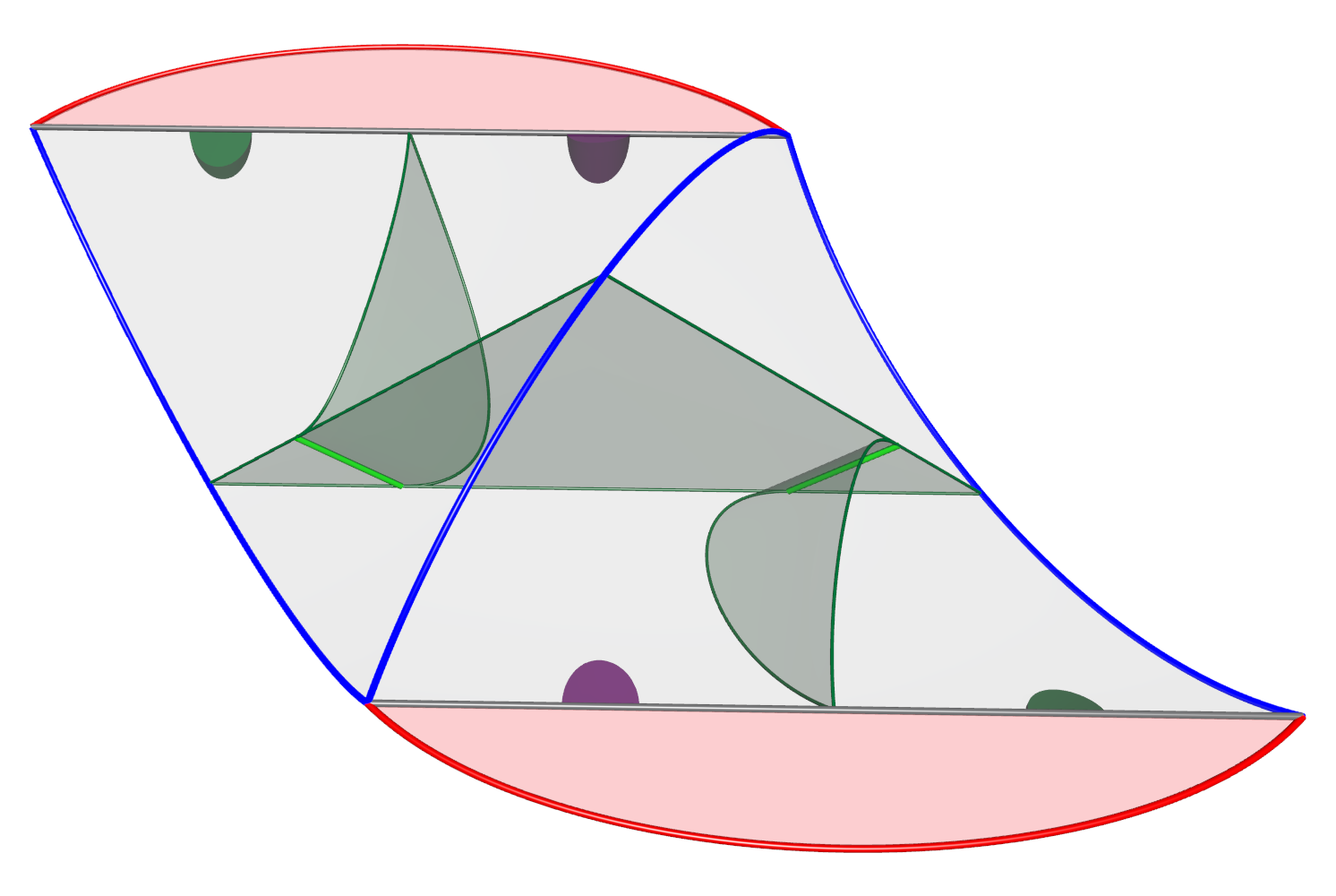
(a) Three-quarter view.

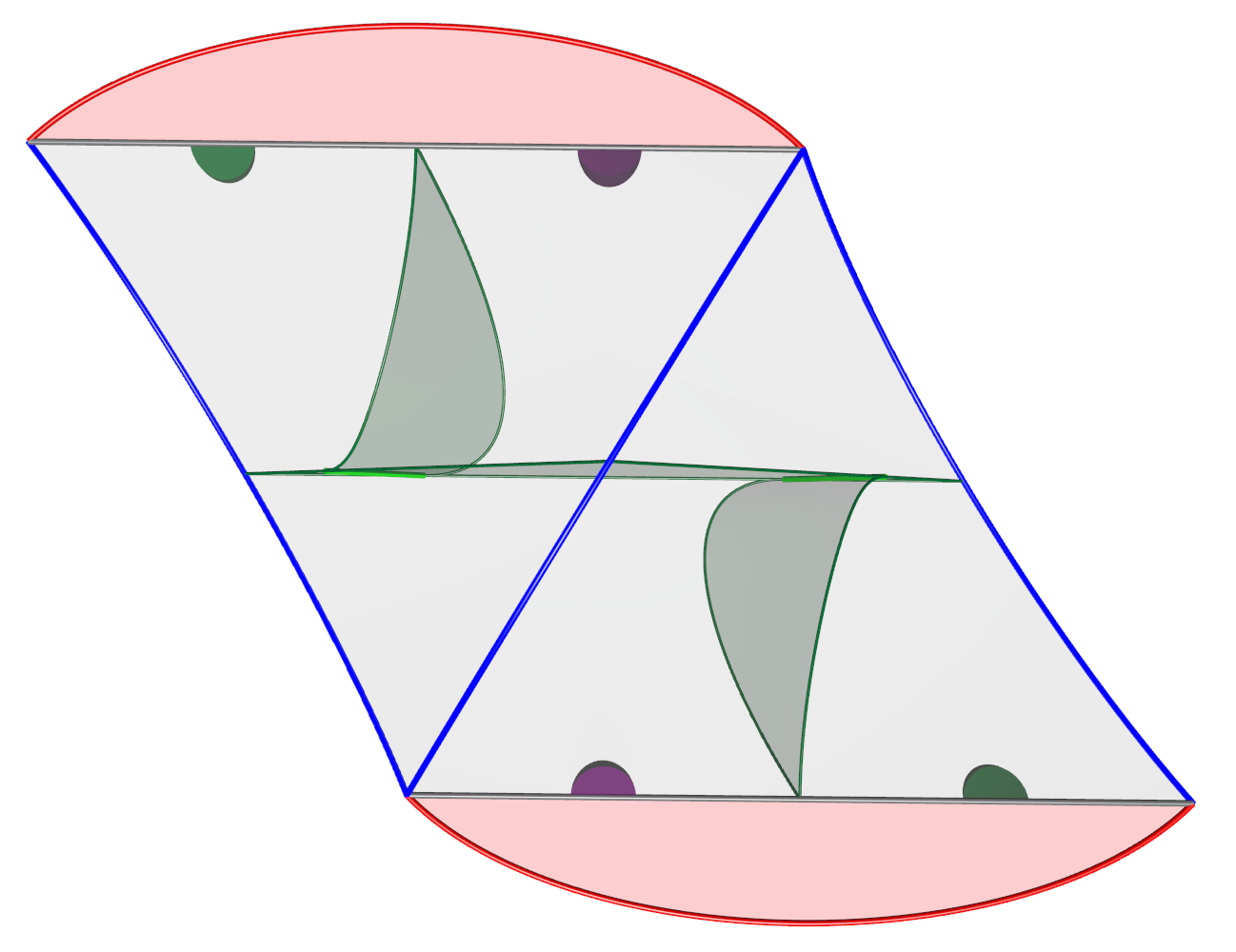
(b) Top view.

Figure 7.1. Straightened $B^{t}$ in an upper half-tetrahedron (toggle or fan).

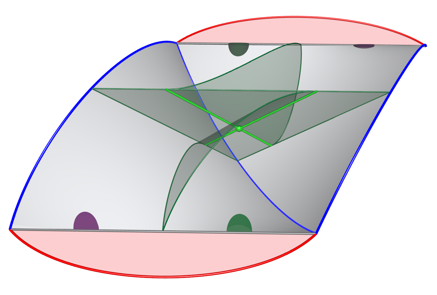
(a) Three-quarter view.

(b) Top view.

Figure 7.2. Straightened $B^{t}$ in a lower half-tetrahedron (fan).

(a) Three-quarter view.

(b) Top view.

Figure 7.3. Straightened $B^{t}$ in a lower half-tetrahedron (toggle).

(a) Three-quarter view.

(b) Top view.

Figure 7.4. Straightened $B^{\mathcal{V}}$ in a crimped shearing region.

We illustrate our construction with a running example. The example is fLLQccecddehqrwjj_20102 , chosen from the veering census [11]. Figure 7.5 shows the result of straightening in this example, in various cross-sections.

Remark 7.1.

In our pictures of cross-sections we shade all toggle squares in grey and all crimped bigons the colour of their veering edge. Along a branch interval of $B^{\mathcal{V}}$ within a crimped solid torus, track-cusps are labelled with the same letter. As we move from an upper boundary to a lower boundary the labels (on track-cusps of $B^{\mathcal{V}}$) advance by one letter. Track-cusps of $B_{\mathcal{V}}$ are indicated with small triangles. ∎

2pt $\partial^{+}\Theta^{\mathcal{V}}$ [r] at 10 1340 $\partial^{-}\Theta^{\mathcal{V}}=\partial^{+}\Theta_{\mathcal{V}}$ [r] at 10 760 $\partial^{-}\Theta_{\mathcal{V}}$ [r] at 10 178

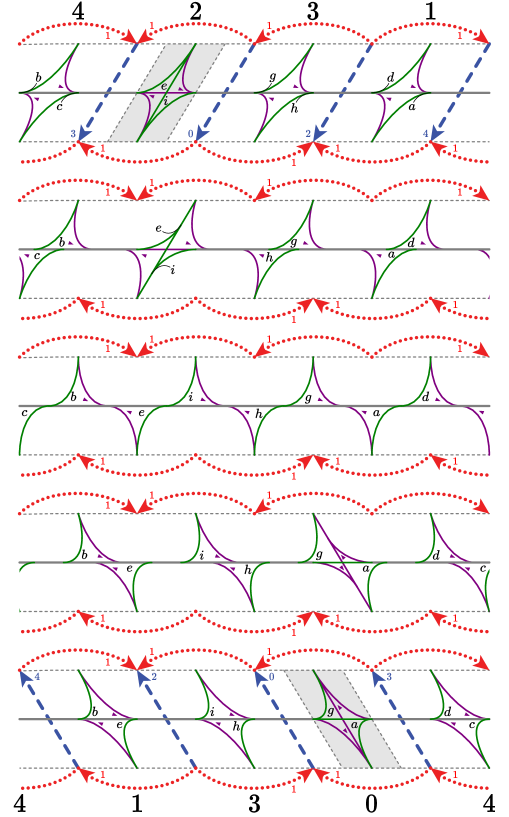
(a) Blue crimped solid torus.

(b) Red.

Figure 7.5. The intersection of $B^{\mathcal{V}}$ (and $B_{\mathcal{V}}$), after straightening, with various horizontal cross-sections of the crimped shearing decomposition of fLLQccecddehqrwjj_20102 . Compare with Figure 5.8. We indicate the position of track-cusps with letters or small triangles; sometimes we use a ‘‘whisker’’ pointing from a letter or triangle to the track-cusp itself. The stations are not drawn.

Remark 7.2.

In Figure 7.5 the upper boundary of the blue crimped solid torus $U$ is glued to the lower boundary of $U$ along the fan squares, by a $180^{\circ}$ rotation and a (left) shear. As a result, the blue helical veering edges and the red longitudinal veering edges (adjacent to fan squares) match on the top and bottom of $U$. The red longitudinal veering edges adjacent to the toggle squares do not match. This is because they are glued to the red crimped solid torus $V$. The upper and lower boundaries of $V$ are also glued, by a $180^{\circ}$ rotation and a (right) shear, along the red crimped bigons. ∎

Remark 7.3.

Suppose that $U$ is a crimped shearing region. Let $H=\partial^{-}U=\partial^{-}\Theta_{U}$ and $K=\partial^{+}U=\partial^{+}\Theta^{U}$. Let $\tau^{H}$ and $\tau^{K}$ be the intersections of $B^{\mathcal{V}}$ with $H$ and $K$, respectively. So $\tau^{H}$ and $\tau^{K}$ are train-tracks. We arrange matters so that $\tau^{H}$ meets longitudinal crimped (helical veering) edges of $H$ with a tangent vector which is parallel to the helical veering (longitudinal crimped) edges of $H$; see Figure 7.5. We do the same for $\tau^{K}$. This ensures that tangent vectors match up when sheared by the gluing maps.

Suppose that $H_{s}$ parametrises the cross-sections of $U$, with $H_{0}=\partial^{-}\Theta_{U}$, with $H_{1/2}=\partial^{+}\Theta_{U}=\partial^{-}\Theta^{U}$ and with $H_{1}=\partial^{+}\Theta^{U}$. As $s$ increases from $0$ to $1$, the tangent vectors of branches meeting longitudinal crimped edges shear. Again, see Figure 7.5. ∎

Remark 7.4.

Observe that all vertices of $B^{\mathcal{V}}$ now lie along the central curves of the middle cross-sections of the crimped shearing regions. That is, the vertices lie in the intersection of

• the middle cross-section $\partial^{-}\Theta^{\mathcal{V}}=\partial^{+}\Theta_{\mathcal{V}}$ and

• the mid-surface $\mathcal{S}=\mathcal{S}_{R}\cup\mathcal{S}_{B}$. ∎

Definition 7.5.

Suppose that $U$ is a crimped shearing region. Let $A=A(U)$ be the mid-band in $U$. Let $U^{\prime}$ equal $U$ minus its longitudinal crimped edges. We define the shearing projection $\rho_{U}\colon U^{\prime}\to A$ as follows.

• In every cross-section, $\rho_{U}$ projects along lines in bigon coordinates.

• In $\partial^{\pm}U$ these lines are parallel to the helical veering edges.

• In the cross-sections between the upper and lower boundaries of $U$ the direction of projection interpolates linearly.

Suppose that $U$ and $V$ are crimped shearing regions of the same colour with $\partial^{+}U$ intersecting $\partial^{-}V$. Then, by construction, $\rho_{U}$ and $\rho_{V}$ agree on $\partial^{+}U^{\prime}\cap\partial^{-}V^{\prime}$ (a union of fan squares and crimped bigons). So, for any union $\mathcal{U}$ of crimped shearing regions, all of the same colour, we may define $\rho_{\mathcal{U}}=\bigcup\rho_{U}$ where the union ranges over $U$ in $\mathcal{U}$. ∎

Remark 7.6.

Suppose that $\mathcal{U}$ is a union of crimped shearing regions, all of the same colour. Suppose that $C$ is the intersection of the branch lines of $B^{\mathcal{V}}$ (in straightened position) with $\mathcal{U}$. We draw the projection $\rho_{\mathcal{U}}(C)$ on the mid-surface $\mathcal{S}_{\mathcal{U}}$ in a particular example in Figure 7.6.

In straightened position, a branch interval (that is, a component of $C$) lies in the mid-surface until slightly below the toggle square it exits through. Thus that sub-interval and its projection under $\rho_{\mathcal{U}}$ agree and are (almost) straight. Just below the exiting toggle square, the track-cusp continues to move at constant speed (with respect to the $x$–coordinate). However, the shearing of the projections exactly cancel that motion. As a result, the projection of the remaining sub-interval is (almost) vertical. Finally, we note that the branch intervals and their projections are smooth curves. What we have drawn in Figure 7.6 is thus a (highly accurate) approximation of the actual position. ∎

(a) Blue mid-surface.

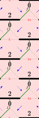
(b) Red.

Figure 7.6. The branch lines of $B^{\mathcal{V}}$, after straightening, projected to (a $\mathbb{Z}^{2}$ cover of each component of) the mid-surface $\mathcal{S}$. Compare with Figure 5.8. Note that we have drawn six fundamental domains, stacked vertically. The projection is drawn with a solid (dotted) line exactly as the corresponding track-cusps is in front of (behind) the branch surface.

Remark 7.7.

As noted in Corollary 3.4 the branched surface $B^{\mathcal{V}}$, when in dual position, is dynamic. Straightening makes parts of $B^{\mathcal{V}}$ vertical. However, the branch locus remains transverse, and not orthogonal, to vertical. Thus the straightened $B^{\mathcal{V}}$ is again dynamic. ∎

7.2. Shrinking

Next we shrink: in each crimped shearing region $U$, we form a very small collar $\Gamma^{U}$ of $\partial^{+}U$, obtained as a union of horizontal cross-sections $Z(p,U)$. Note that $\Gamma^{U}$ is disjoint from the vertices of $B^{\mathcal{V}}$. We now move $B^{\mathcal{V}}$ by a proper isotopy of $U$ which preserves $x$ and $y$ coordinates (in bigon coordinates) and permutes the cross-sections $Z(p,U)$. The isotopy carries the bottom of $\Gamma^{U}$ downwards to $\partial^{-}\Theta^{U}$ and evenly redistributes the cross-sections below $\Gamma^{U}$ inside of $\Theta_{U}$.

Before the isotopy, $B^{\mathcal{V}}$ was transverse to the equatorial squares. After the isotopy, $B^{\mathcal{V}}$ is almost vertical in all of $\Theta^{U}$. The intersections of $B^{\mathcal{V}}$ with $\partial^{+}U$ and $\partial^{-}U$ are unchanged by the shrinking isotopy. Note that the shrinking isotopy maintains the $180^{\circ}$ symmetry of the branched surfaces $B^{t}$. In Figure 7.7 we show the intersection of the shrunken $B^{\mathcal{V}}$ (and $B_{\mathcal{V}}$) with various horizontal cross-sections.

2pt $\partial^{+}\Theta^{\mathcal{V}}$ [r] at 10 1340 $\partial^{-}\Theta^{\mathcal{V}}=\partial^{+}\Theta_{\mathcal{V}}$ [r] at 10 760 $\partial^{-}\Theta_{\mathcal{V}}$ [r] at 10 178

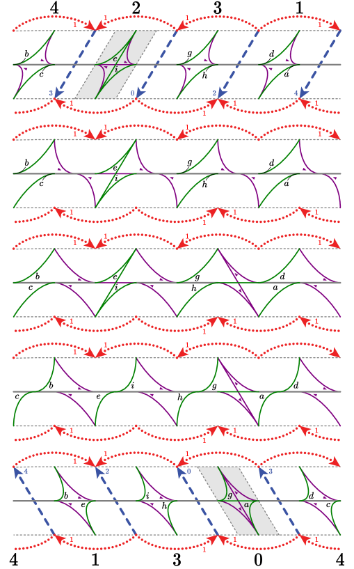
(a) Blue crimped solid torus.

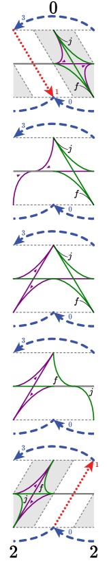
(b) Red.

Figure 7.7. The intersection of $B^{\mathcal{V}}$ (and $B_{\mathcal{V}}$), after shrinking, with various horizontal cross-sections of the crimped shearing decomposition of fLLQccecddehqrwjj_20102 . Compare with Figure 7.5.

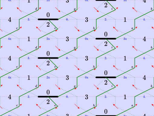
(a) Blue mid-surface.

(b) Red.

Figure 7.8. The branch lines of $B^{\mathcal{V}}$, after shrinking, projected to the mid-surfaces. Compare with Figure 7.6.

Remark 7.8.

Note that the shearing of tangent vectors, as in Remark 7.3, now occurs in $\Theta_{\mathcal{V}}$ for $B^{\mathcal{V}}$ (and in $\Theta^{\mathcal{V}}$ for $B_{\mathcal{V}}$). ∎

Remark 7.9.

Shrinking permutes cross-sections; thus by Remark 7.7 the shrunken branched surface $B^{\mathcal{V}}$ is again dynamic. ∎

8. Parting

Here we define the parting isotopies. These are applied to the upper and lower branched surfaces $B^{\mathcal{V}}$ and $B_{\mathcal{V}}$, placing them in parted position. These isotopies are almost local: in each tetrahedron, outside of the stations, they depend only on the combinatorics of that tetrahedron and its immediate neighbours. The way in which the branched surface intersects crimped edges inside of stations is more delicate and is dealt with in Section 8.3.

Concentrating on $B^{\mathcal{V}}$, we now sketch the construction before giving the details. We start in shrunken position (shown in Figure 7.7). In each cross-section of $\Theta^{\mathcal{V}}$, and near each crimped edge, we will move $B^{\mathcal{V}}$ towards a chosen station (corner) of the relevant toggle square. We will also isotope branches of $B^{\mathcal{V}}$ in cross-sections of $\Theta^{\mathcal{V}}$ to be (almost) line segments (in bigon coordinates). As for shrunken position, the parted position of $B^{\mathcal{V}}$ in $\Theta^{\mathcal{V}}$ will be almost a product.

This done, we will move $B^{\mathcal{V}}$ downward in $\Theta_{\mathcal{V}}$. This makes the intersection of $B^{\mathcal{V}}$ with the cross-sections into a sequence of train-tracks as follows. As they move up through $\Theta_{\mathcal{V}}$ they first perform a splitting of the track-cusps along their parting routes. They next perform a graphical isotopy where the track-cusps are (almost) motionless and the branches straighten to become (almost) line segments.

The branched surface $B_{\mathcal{V}}$ moves in a similar way but swapping $\Theta^{\mathcal{V}}$ and $\Theta_{\mathcal{V}}$. The combined procedure of splitting along routes and graphical isotopy will be used once (in space) in this section and three more times (twice in time and once in space) in Section 9. We use these to fill in the isotopy from parted position to their final draped position.

2pt $\partial^{+}\Theta^{\mathcal{V}}$ [r] at 10 1340 $\partial^{-}\Theta^{\mathcal{V}}=\partial^{+}\Theta_{\mathcal{V}}$ [r] at 10 760 $\partial^{-}\Theta_{\mathcal{V}}$ [r] at 10 178

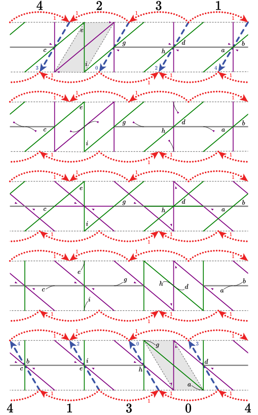
(a) Blue crimped solid torus.

(b) Red.

Figure 8.1. The intersection of $B^{\mathcal{V}}$ (and $B_{\mathcal{V}}$), after parting, with various cross-sections of the crimped shearing decomposition of fLLQccecddehqrwjj_20102 . The branched surfaces intersect the longitudinal crimped edges within stations. As in Figure 7.7, the branched surface $B^{\mathcal{V}}$ is almost vertical in $\Theta^{\mathcal{V}}$. Likewise, $B_{\mathcal{V}}$ is almost vertical in $\Theta_{\mathcal{V}}$.

(a) Blue mid-surface.

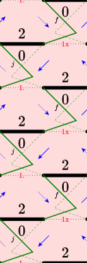
(b) Red.

Figure 8.2. The branch lines of $B^{\mathcal{V}}$, after parting, projected to the mid-surfaces. Compare with Figure 7.8.

8.1. Parting in $\Theta^{\mathcal{V}}$

We now describe the parting isotopy in $\Theta^{\mathcal{V}}$.

Suppose that $U$ is a crimped blue shearing region. Suppose that $e^{\prime}$ is a longitudinal crimped edge for $U$. Suppose that $e$ is the associated red veering edge and let $C$ be the crimped bigon which $e$ and $e^{\prime}$ cobound. Suppose that $S$ is the upper toggle square meeting $e^{\prime}$. We equip $C$ with the anti-clockwise orientation, as viewed from above. This induces orientations on $e$ and $e^{\prime}$. Let $c=C\cap B^{\mathcal{V}}$. The parting isotopy in $\Theta^{U}$ fixes $c\cap e$ and moves $c\cap e^{\prime}$ along $e^{\prime}$, against the orientation of $e^{\prime}$ (given just above), until it arrives at the station cutting off the cusp of the toggle square $S$. (If, instead, $U$ is red, then we move $c\cap e^{\prime}$ along $e^{\prime}$, following the orientation of $e^{\prime}$, again until it arrives at its station.) To see this motion, compare top lines of Figures 7.7 and 8.1.

In $\partial^{+}U$ we also move track-cusps outwards in fan squares until they arrive close to the midpoint of a helical edge. In other cross-sections of $\Theta^{U}$ we do the same, but now moving track-cusps until they almost meet the projection (in bigon coordinates) of the midpoint of a helical edge.

Remark 8.1.

Thus $B^{\mathcal{V}}$ is almost a product in $\Theta^{U}$. The track-cusps move very slowly forward in cross-sections to preserve dynamism. Track-cusps outside of stations all move at the same speed. The motion of track-cusps inside of stations is described in Section 8.3. Where a train-track meets a longitudinal crimped edge, its tangent vector remains parallel to the (projection of the) helical veering edges in $\partial^{+}U$. See Remark 7.8. ∎

Remark 8.2.

Parting in $\Theta^{\mathcal{V}}$ determines parted position in $\partial^{-}\Theta_{\mathcal{V}}$. The general picture is shown in Figure 8.3. The running example shows a particular case – see the bottom row of Figure 8.1. ∎

Remark 8.3.

Once in parted position, in any cross-section the train-track intersects crimped edges only within stations. Again, the exact location where a branch intersects a crimped edge within a station is set in Section 8.3. ∎

Remark 8.4.

Outside of stations, the parting isotopy in $\Theta^{U}$ depends only on whether a branch is below a toggle square or a fan square in $\partial^{+}U$. ∎

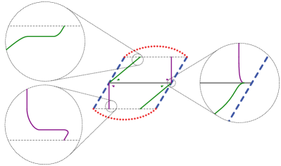
(a) Fan square in $\partial^{+}U$.

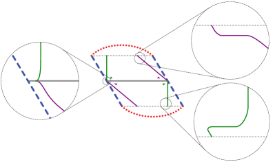
(b) Fan square in $\partial^{-}U$.

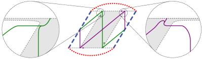
(c) Toggle square in $\partial^{+}U$.

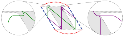
(d) Toggle square in $\partial^{-}U$.

Figure 8.3. In parted position the intersections of $B^{\mathcal{V}}$ and $B_{\mathcal{V}}$ with cross-sections are line segments except for (a) inside of the stations and (b) very close to the midpoints of helical edges. Note that here $U$, the containing crimped shearing region, is blue.

8.2. Graphical tracks and isotopies

In order to organise isotopies in cross-sections in $\Theta_{\mathcal{V}}$ we require the following.

Definition 8.5.

Suppose that $U$ is a crimped shearing region. Suppose that $H$ is a cross-section in $\Theta_{U}$. We consider the foliation of $H$ by lines (in bigon coordinates) parallel to the helical veering edges in $\partial^{-}U$. We say that a smooth arc $\alpha$ in $H$ is lower graphical if $\alpha$ is transverse to this foliation (except possibly at its endpoints). Suppose that $\tau$ is a train-track in $H$. If all branches of $\tau$ are lower graphical then we say that $\tau$ is lower graphical.

We define upper graphical for cross-sections in $\Theta^{U}$ using the helical veering edges in $\partial^{+}U$. If a track is upper or lower graphical we simply call it graphical. ∎

The definition implies the following.

Lemma 8.6.

Suppose that $\tau$ is a graphical train-track. Suppose that $\alpha$ is a train route in $\tau$. Then the result of splitting $\tau$ along $\alpha$, in a small neighbourhood of $\alpha$, is again graphical. ∎

Lemma 8.7.

Suppose that $B^{\mathcal{V}}$ is in parted position in $\Theta^{\mathcal{V}}$ (and thus in $\partial^{-}\Theta_{\mathcal{V}}$). Suppose that $H$ is either a cross-section in $\Theta^{\mathcal{V}}$ or in $\partial^{-}\Theta_{\mathcal{V}}$. Then the track $\tau^{H}=B^{\mathcal{V}}\cap H$ is lower graphical.

Proof.

Suppose that $H$ is a cross-section in $\partial^{+}\Theta^{\mathcal{V}}$. As discussed in Remark 8.4, parted position of $\tau^{H}$ (outside of stations) is defined locally. Also, as shown in Figure 8.3 all branches of $\tau^{H}$ outside of stations are straight and not parallel to the lower helical slope. Thus, outside of stations, all branches of are lower graphical. Inside of stations branches of $\tau^{H}$ are laid out according to Figures 8.3a and 8.3c; these are also lower graphical.

A similar argument, referring instead to Figures 8.3b and 8.3d, deals with the case where $H=\partial^{-}\Theta_{\mathcal{V}}$.

Finally suppose that $H$ is a cross-section inside of $\Theta^{\mathcal{V}}$. By Remark 8.1, the train-track $\tau^{H}$ is a projection (in bigon coordinates) of a (very slight) folding of the train-track in $\partial^{+}\Theta^{\mathcal{V}}$. Thus $\tau^{H}$ is again lower graphical. ∎

Definition 8.8.

Suppose that $H$ is a cross-section. Suppose that $b$ and $b^{\prime}$ are arcs in $H$ transverse to the lower foliation. Suppose that $b$ and $b^{\prime}$ have the same endpoints. The graphical isotopy of $b$ to $b^{\prime}$ is as follows. For every leaf $\ell$ of the lower foliation intersecting $b$, we move the point $b\cap\ell$ to the point $b^{\prime}\cap\ell$, along $\ell$, at constant speed so that its journey takes the entire time of the isotopy. ∎

8.3. Junctions

We introduce junctions as well as their heights and widths. We use these dimensions to determine the position of the siding inside of a junction, as well as its decomposition into blocks. This allows us to describe the intersection of the branched surface with a (small neighbourhood of a) longitudinal edge. This will resolve the issues raised in Remarks 8.1 and 8.3.

Remark 8.9.

The exact geometry of junctions is only used to make sure that track-cusps always move forward and never “overtake” each other, and to ensure that the branched surfaces do not have “accidental” intersections. The material on junctions, sidings, and blocks can safely be ignored on a first reading. ∎

Definition 8.10.

Suppose that $\Sigma$ is an upper station. Suppose that $S$ is a toggle square intersecting $\Sigma$. The upper junction $J=J(\Sigma,S)$ is obtained as follows. Suppose that $S^{\prime}$ is the next toggle square that $\Sigma$ intersects, travelling downwards from $S$. Let $U$ and $U^{\prime}$ be the crimped shearing regions directly below $S$ and directly above $S^{\prime}$. Then $J=J(\Sigma,S)$ is the (closure in the path metric of the) component of $\Sigma-(\partial^{+}U\cup\partial^{-}U^{\prime})$ intersecting $U$ and $U^{\prime}$. The height of $J$, denoted $h_{J}$, is the number of crimped shearing regions whose interior it intersects. Note that the height is finite by Lemma 2.2. We define lower junctions, and their heights, similarly. ∎

For the rest of this section, we fix the following. Suppose that $J=J(\Sigma,S)$ is the upper junction associated to the station $\Sigma$ and the toggle square $S$. Let $U$ be the crimped shearing region directly below $S$. Let $e$ be the crimped longitudinal edge of $U$ that intersects $J$.

Definition 8.11.

Let $c$ be the cusp of $e$ closest to $J$. Let $e^{\prime}$ be the other crimped longitudinal edge of $U$ meeting $c$. See Figure 5.11. Let $J^{\prime}$ be the upper junction intersecting $U$ and $e^{\prime}$. The width of $J$, denoted $w_{J}$, is defined to be the height of $J^{\prime}$. We make a similar definition for lower junctions. ∎

In the following definition it will be useful to consult Figure 5.11b.

Definition 8.12.

Let $c$ be the cusp of $e$ closest to $J$. Let $e^{\prime}$ be the other crimped longitudinal edge of $U$ meeting $c$. Let $J^{\prime}$ be the lower junction intersecting $U$ and $e^{\prime}$. Let $c^{\prime}$ be the other cusp of $e$. Let $e^{\prime\prime}$ be the other longitudinal crimped edge of $U$ meeting $c^{\prime}$. Let $J^{\prime\prime}$ be the upper junction intersecting $U$ and $e^{\prime\prime}$. We take $\epsilon$ to be a small universal constant (smaller than the “slightly more” used in Remark 6.1(3)). The radius of $J$, denoted $r_{J}$, is defined to be $\epsilon$ divided by the larger of

$$h^{\prime}+w^{\prime}\quad\mbox{and}\quad h^{\prime\prime}+w^{\prime\prime}$$

where these are the heights and widths of $J^{\prime}$ and $J^{\prime\prime}$ respectively. We make a similar definition for lower junctions. ∎

We use this to control the cross-sectional radius of stations (Definition 5.12). Suppose that $\Sigma$ is a station. Suppose that $J$ is a junction contained in $\Sigma$. Let $S^{\prime}$ be the toggle square meeting the lower boundary of $J$. Let $U^{\prime}$ be the crimped shearing region immediately above $S^{\prime}$. For any cross-section $H$ meeting $J$ other than those in the lower $1/8^{\rm th}$ of $U^{\prime}$, the radius of $J\cap H$ is $r_{J}$. The junction $J$ meets two other junctions along $\partial^{-}U^{\prime}$, say $J^{\prime}$ through $S^{\prime}$ and $J^{\prime\prime}$ not. In the lower $1/16^{\rm th}$ of $U^{\prime}$ the radius of $J\cap H$ is the larger of $r_{J^{\prime}}$ and $r_{J^{\prime\prime}}$. In the second $1/16^{\rm th}$ of $U^{\prime}$ the radius interpolates linearly between its values at its top and bottom.

Definition 8.13.

Let $e^{\prime}$ be the helical crimped edge in $\partial^{+}U$ which intersects $J$. Let $b$ be the branch of $B^{\mathcal{V}}\cap\partial^{+}U$ (in parted position) that intersects $e^{\prime}$. Let $p$ be the point of intersection between $b$ and $e^{\prime}$. Let $h_{J}$ and $w_{J}$ be the height and width of $J$ respectively. We set the $y$-coordinate of $p$ to be $r_{J}/(2h_{J}+w_{J})$, as measured in bigon coordinates from $e$. See Figure 8.4.

Outside of a small neighbourhood of the longitudinal crimped edges, the helical crimped edge $e^{\prime}$ is a line segment in $\partial^{+}U$. Extend this line (in bigon coordinates) until it intersects $e$ at a point $q$. We take $p^{\prime}$ to be the point of intersection between $x(p,U)$ and $y(q,U)$. Twice the distance between $p$ and $p^{\prime}$, along $x(p,U)$, is the block length, denoted $b_{J}$. The point $p^{\prime}$ is the last block boundary. The siding in $J$ is the component of $\big{(}x(p^{\prime},U)\cap J\big{)}-p^{\prime}$ containing $p$. The other block boundaries are the points of the siding which are an integer multiple of the block length away from $p^{\prime}$. The segments of the siding between block boundaries are called blocks. See Figure 8.4. ∎

2pt $e$ [l] at 35 207 $e^{\prime}$ [l] at 35 180 $b$ [l] at 35 147 $q$ [b] at 207 202 $p^{\prime}$ [t] at 207 160 $p$ [tr] at 151 145

Figure 8.4. The block boundaries are marked by black dots, with the last block boundary inside of the toggle square $S$. The labels are used in Definition 8.13.

Remark 8.14.

Note that each crimped edge appears in the various crimped shearing regions as a helical crimped edge exactly twice, and otherwise as a longitudinal crimped edge. When it appears as a helical crimped edge, it is once on an upper boundary of a crimped shearing region (see Figure 8.3c), and once on a lower boundary (see Figure 8.3d). Thus Definition 8.13 is well-defined. ∎

With conventions (on bigon coordinates) as given in Remark 6.1 the block length for $J$ is

$$b_{J}=\frac{2}{\sqrt{3}}\cdot\frac{r_{J}}{2h_{J}+w_{J}}$$

Let $(U_{i})_{i=1}^{N}$ be the crimped shearing regions meeting the interior of $J$. Thus $U_{1}=U^{\prime}$ and $U_{N}=U$. Let $H$ be a cross-section of any one of the $U_{i}$ other than in the lowest $1/8^{\rm th}$ of $U_{1}$. We project the siding and its blocks downward (using bigon coordinates) to obtain a siding, and its blocks, in $H$. The projection from $U_{i+1}$ down to $U_{i}$ has the effect of shearing the blocks back by a single block length. The distance between the siding and the longitudinal edge does not change. By our choice of radius the siding in $J\cap H$ contains $2h_{J}+w_{J}$ blocks. The train track in $J\cap H$, in parted position, is required to contain all of these blocks. (If $H$ lies in the lowest $1/16^{\rm th}$ of $U_{1}$ then the siding of $J\cap H$ is inherited from the junction immediately below $J\cap\partial^{-}U_{1}$ not meeting the toggle square. In the second $1/16^{\rm th}$ we interpolate.)

Recall that the toggle square $S$ lies in $\partial^{+}U$. Let $H_{s}$, for $s\in[1/2,1]$ be the cross-section of $\Theta^{U}$ at height $s$ in bigon coordinates. Let $k$ be the track-cusp of $B^{\mathcal{V}}\cap H_{1}$ (in parted position) contained in $J$. Let $K$ be the branch line running through $k$. Let $k_{s}=K\cap H_{s}$. We require that $k_{s}$ lies in the last block of the siding in $J\cap H_{s}$. Furthermore we require that $k_{1/2}$ lies at the middle of the block while $k_{1}$ meets the last block boundary. Finally, we require that the $k_{s}$ move at constant speed.

8.4. Parting routes

Fix $U$ a crimped shearing region. Let $H_{s}$, for $s\in[0,1/2]$ be the cross-section of $\Theta_{U}$ at height $s$ in bigon coordinates. We describe the parted position of $B^{\mathcal{V}}$ in $\Theta_{U}$ as an isotopy of the train-tracks $\tau^{s}=B^{\mathcal{V}}\cap H_{s}$. As $s$ ranges over $[0,1/4]$ we will split the tracks along parting routes. As $s$ ranges over $[1/4,1/2]$ we will perform a graphical isotopy. We now turn to the details.

Definition 8.15.

Suppose that $k$ is a track-cusp of $B^{\mathcal{V}}\cap\partial^{-}U$, whose position is determined by Remark 8.2. Let $K$ be the branch line of $B^{\mathcal{V}}$ (in shrunken position) determined by $k$. Let $\ell$ be the track-cusp of $K$ lying in $\partial^{+}U$, in prepared position. Let $\ell^{\prime}$ be the projection of $\ell$ (via bigon coordinates) to $\partial^{-}U$. Then the parting route $\alpha(k)$ is the unique route from $k$ to (just before) $\ell^{\prime}$ carried by the parted track in $\partial^{-}U$.

When $\ell^{\prime}$ lies in a junction (equivalently, if $\ell$ lies in a toggle square), the route $\alpha(k)$ ends in the same block as $\ell^{\prime}$, but three-quarters of a block length before $\ell^{\prime}$. ∎

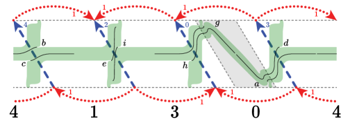
(a) Blue crimped solid torus.

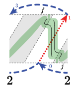
(b) Red.

(c) The sixth case.

Figure 8.5. Parting routes for the track-cusps in $\partial^{-}\Theta_{\mathcal{V}}$, where $\mathcal{V}$ is fLLQccecddehqrwjj_20102 . Here we draw a regular neighbourhood of the train-track in green. Compare with the last line of Figure 8.1.

By Remark 8.4, the parting isotopy in $\Theta^{\mathcal{V}}$ is local (outside of stations). Thus there are only finitely many (in fact six) combinatorial possibilities for $\alpha(k)$. These are all shown in Figure 8.5.

• Suppose that $\ell$ lies in a toggle square in $\partial^{+}U$.

  • If $k$ also lies in a toggle square (in $\partial^{-}U$) then we obtain the examples $f$ and $j$ in Figure 8.5b.

  • Otherwise $k$ does not lie in a toggle square and we obtain the examples $e$ and $i$ in Figure 8.5a.

• Suppose that $\ell$ does not lie in a toggle square.

  • Suppose that $\ell^{\prime}$ lies in a toggle square.

    • If $k$ lies in a toggle square then we obtain the examples shown in Figure 8.5c.

    • Otherwise $k$ does not lie in a toggle square and we obtain the examples $d$ and $h$ in Figure 8.5a.

  • Suppose that $\ell^{\prime}$ does not lie in a toggle square.

    • If $k$ lies in a toggle square then we obtain the examples $a$ and $g$ in Figure 8.5a.

    • Otherwise $k$ does not lie in a toggle square and we obtain the examples $b$ and $c$ in Figure 8.5a.

8.5. Splitting along parting routes

Suppose that $U$ is a crimped shearing region. Let $H_{s}$ be the family of cross-sections of $\Theta_{U}$, with $H_{0}=\partial^{-}\Theta_{U}$ and $H_{1/2}=\partial^{+}\Theta_{U}$. Recall that $B^{\mathcal{V}}$ in parted position is already specified in $H_{0}$ and $H_{1/2}$. Instead of parametrising the parting isotopy explicitly, we specify parted position in $B^{\mathcal{V}}\cap H_{s}$ by giving a family of train-tracks.

2pt $\partial^{+}\Theta_{\mathcal{V}}$ [r] at 10 1327 Graphical isotopy at -120 1040 Splitting along parting routes at -120 470 $\partial^{-}\Theta_{\mathcal{V}}$ [r] at 10 179

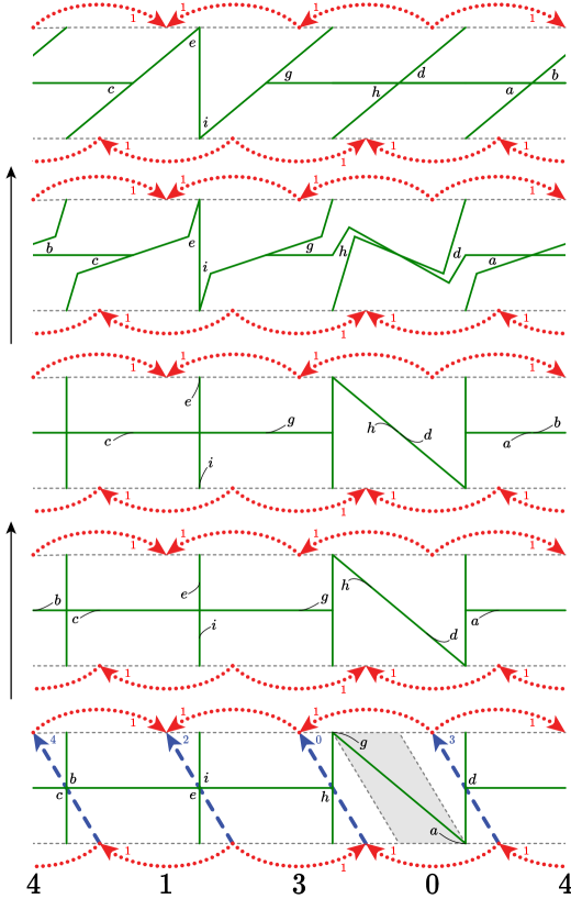
(a) Blue crimped solid torus.

(b) Red.

Figure 8.6. The result $B_{1}$ of the parting isotopy in $\Theta_{\mathcal{V}}$ where $\mathcal{V}$ is fLLQccecddehqrwjj_20102 . The five diagrams show (from the bottom moving up) $B_{1}\cap C_{s}$ for $s\in(0,1/8,1/4,3/8,1/2)$. Thus this figure interpolates the lower three lines of Figure 8.1. The bottom cross-section contains blue helical edges.

As $s$ ranges over $[0,1/4]$ the intersections of $B^{\mathcal{V}}$ (in parted position) with the cross-sections $H_{s}$ show a movie of a splitting along all of the parting routes. In detail: if $k$ is a track-cusp in $H_{0}$ we split $k$ forward in a small neighbourhood of its parting route $\alpha(k)$. The result in an example is shown in the lower three rows of Figure 8.6. When two track-cusps $k$ and $\ell$ meet, travelling in opposite directions, they split past each other. (If $U$ is blue and there is (not) a toggle square above, this is a left (right) split. If $U$ is red the directions swap.) Outside of stations each track-cusp moves so that

• its $x$--coordinate moves at constant speed and

• its journey takes all of $[0,1/4]$.

Inside of stations we follow the same rule with one exception; track-cusps inside of toggle squares split to the boundary of their square and then move as above. See Figure 8.3c.

The construction of the parting routes (Definition 8.15) implies that track-cusps in $H_{1/4}$ either lie very near to the centre line of the cross-section or lie in stations. See the middle row of Figure 8.6. This describes splitting along the parting routes.

8.6. The graphical isotopy for parted position

Remark 8.16.

Let $\tau^{1/4}$ be the train-track in $H_{1/4}$ given by splitting along parting routes. Lemmas 8.7 and 8.6 ensure that all branches of $\tau^{1/4}$ are lower graphical. Where $\tau^{1/4}$ meets a longitudinal crimped edge, its tangent vector is parallel to the (projection of the) helical veering edges in $\partial^{-}U$.

Let $\tau^{1/2}$ be the train-track in $H_{1/2}$ given by parted position in $\Theta^{U}$. Lemma 8.7 implies that $\tau^{1/2}$ is lower graphical. Where $\tau^{1/2}$ meets a longitudinal crimped edge, its tangent vector is parallel to the (projection of the) helical veering edges in $\partial^{+}U$. ∎

For $s\in[1/4,1/2]$, we perform a lower graphical isotopy from $\tau^{1/4}$ to $\tau^{1/2}$, as follows. By Remark 8.16 both train-tracks are lower graphical. Also they are combinatorially isomorphic and their track-cusps are in (almost) the same places in bigon coordinates.

We now isotope $\tau^{1/4}$ to $\tau^{1/2}$ as follows.

• We move each track-cusp slightly forward from its position in $\tau^{1/4}$ to its position in $\tau^{1/2}$.

• At the same time we perform a lower graphical isotopy (as in Definition 8.8), moving every branch from its position in $\tau^{1/4}$ to its position in $\tau^{1/2}$. This isotopy also changes the tangent vector where $\tau^{s}$ meets a longitudinal crimped edge. See Figure 8.6b.

Points move at constant speed so that their journey takes all of $[1/4,1/2]$. This describes the lower graphical isotopy from $\tau^{1/4}$ to $\tau^{1/2}$.

An example is given in the upper three rows of Figure 8.6.

Lemma 8.17.

The branched surface $B^{\mathcal{V}}$ in parted position is dynamic and is isotopic to shrunken position.

Proof.

The intersection with each cross-section is a train-track. Moreover, by construction the track-cusps always move forwards as we move up through cross-sections. Therefore the branched surface is dynamic.

In Section 8.1 we explicitly describe the isotopy between the shrunken branched surface and the parted branched surface in $\Theta^{\mathcal{V}}$. Thus in $\Theta_{\mathcal{V}}$ the shrunken branched surface and the constructed branched surface meet $\partial^{-}\Theta_{\mathcal{V}}$ and $\partial^{+}\Theta_{\mathcal{V}}$ with the same combinatorics. Thus the constructed branched surface is isotopic to the shrunken branched surface. ∎

We call the result parted position for $B^{\mathcal{V}}$. We define parted position for the lower branched surface $B_{\mathcal{V}}$ analogously.

9. Draping

Here we define the draping isotopies. These are applied to the upper and lower branched surfaces $B^{\mathcal{V}}$ and $B_{\mathcal{V}}$ starting from parted position and ending in draped position.

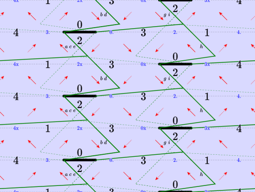
(a) Blue mid-surface.

(b) Red.

Figure 9.9. The branch lines of $B^{\mathcal{V}}$, in draped position, projected to the mid-surfaces. Compare with Figure 8.2.

As usual we concentrate on the upper case. The name draped comes from the final position of the branch lines. Suppose that $C$ is a branch line. Suppose that $\mathcal{U}$ is a component of the monochromatic decomposition, as in Definition 5.13. Suppose that $C^{\prime}=C\cap\mathcal{U}$ is a branch interval. Suppose that the initial point of $C^{\prime}$ lies in $\partial^{-}\Theta_{U}$: here $U$ is a crimped shearing region in $\mathcal{U}$. In draped position $C^{\prime}$ runs just above $\partial^{-}\Theta_{U}$, until it encounters the downwards projection (in bigon coordinates) of a toggle square. At that point $C^{\prime}$ moves sharply upwards to get just above that toggle square. The process then repeats until $C^{\prime}$ exits $\mathcal{U}$ through some toggle square. Thus the image of $C^{\prime}$, under the shearing projection into the midsurface (Definition 7.5), is ‘‘draped’’ over the images of the toggle squares. See Figure 9.9 for the images of the draped branch intervals in our running example.

We begin with an outline of the construction. The branched surface $B^{\mathcal{V}}$ begins in parted position, as provided in Section 8. Justifying Remark 1.4, the draping isotopy is fixed on the union of the toggle squares. That is, it is fixed on the boundaries of the components of the monochromatic decomposition.

We use $B^{\mathcal{V}}_{t}$ to denote the image of $B^{\mathcal{V}}$ at time $t\in[0,1]$. In $\Theta^{\mathcal{V}}$, where $B^{\mathcal{V}}_{0}$ is almost a product, on each cross-section we will perform (in time)

• an almost identical splitting along the draping routes, and

• an almost identical lower graphical isotopy.

This will determine $B^{\mathcal{V}}_{t}\cap\Theta^{\mathcal{V}}$ for all $t$, and thus will fix $B^{\mathcal{V}}_{t}\cap\partial^{\pm}\Theta_{\mathcal{V}}$.

As with the parting isotopy, the motion in the interior of $\Theta_{\mathcal{V}}$ is significantly more complicated. Suppose that $U$ is a crimped shearing region. To build $B^{\mathcal{V}}_{1}\cap\Theta_{U}$ we start from $B^{\mathcal{V}}_{1}\cap\partial^{-}\Theta_{U}$. Let $H_{1/4}$ be the central cross-section of $\Theta_{U}$. We will perform (in space)

• a splitting along suffix routes to produce $B^{\mathcal{V}}_{1}\cap H_{1/4}$ followed by

• a lower graphical isotopy to $B^{\mathcal{V}}_{1}\cap\partial^{+}\Theta_{U}$.

Finally, suppose that $H_{s}$ is any cross-section of $\Theta_{U}$. To build $B^{\mathcal{V}}_{t}\cap H_{s}$ we start from $B^{\mathcal{V}}_{0}\cap H_{s}$. We will then perform (in time)

• a splitting along prefix routes to produce $B^{\mathcal{V}}_{1/2}\cap H_{s}$ followed by

• a lower graphical isotopy to $B^{\mathcal{V}}_{1}\cap H_{s}$.

In Figure 9.1 we indicate in the domain of the isotopy which splitting routes are used where and when, and also the supports of the lower graphical isotopies.

2pt $\alpha$ [r] at 10 95 $\beta$ [t] at 170 10 $\beta$ [t] at 170 388 $\beta$ [t] at 170 460 $\beta$ [t] at 170 532 $\gamma$ [l] at 625 95 $\delta$ [t] at 170 98 $\delta$ [t] at 170 170 $\delta$ [t] at 170 242

Figure 9.1. The domain of the draping isotopy into $U$. The time coordinate $t$ runs from left to right in the interval $[0,1]$; the space coordinate $s$ runs from bottom to top in the interval $[0,1]$. The dashed line separates the preimage of $\Theta^{U}$ from that of $\Theta_{U}$. The labels $\alpha$, $\beta$, $\gamma$, and $\delta$ indicate the parting, draping, suffix, and prefix routes used for the four splittings. The shaded intervals and region are the supports of the lower graphical isotopies.

9.1. Draping routes

Definition 9.1.

Suppose that $B^{\mathcal{V}}$ is in parted position. Suppose that $K$ is a branch line. Suppose that $U$ is a crimped shearing region. Suppose that $K$ intersects $\partial^{-}U$ at a point $k_{0}$. Starting at $k_{0}$, we follow $K$ upwards until it hits, for the first time, a toggle square $S=S(k_{0})$ not containing $k_{0}$. (This exists by Lemma 2.2.) Let $N$ be the number of crimped shearing regions meeting $K$ strictly between $k_{0}$ and $S$. Let $k_{N}$ be the intersection of $K$ and $S$. Note that $N$ is bounded from above by the height of the junction containing $k_{N}$.

Denote these crimped shearing regions as $U_{i}$ with increasing index as we ascend $K$, starting with $U=U_{1}$. Let $k_{i}$ be the intersection of $K$ with $\partial^{+}U_{i}$. Thus $S$ lies in $\partial^{+}U_{N}$. We parametrise the subinterval $[k_{0},k_{N}]$ of $K$ by $[0,N]$ so that $[i,i+1]$ maps to $[k_{i},k_{i+1}]$.

We now define the draping routes $\beta(k_{r})$ for $r\in[0,N]$ by a (downwards) recursion. As our base case, we take $\beta(k_{N})$ to be the train route with length zero carried by $B^{\mathcal{V}}_{0}\cap\partial^{+}U_{N}$ which starts and ends at $k_{N}$. Since $\beta(k_{N})$ has length zero, it consists only of a tangent vector based at $k_{N}$ and pointing away from the track-cusp. See the station shown on the left-hand side of Figure 8.3c.

Fix $r$ and $s$ in $[0,N]$ with $r<s$. Suppose that $[k_{r},k_{s}]$ is contained inside of $U_{i}$, one of the crimped shearing regions. Thus $i\leq r<s\leq i+1$. Let $H_{r}$ ($H_{s}$) be the cross-section of $U_{i}$ through $k_{r}$ ($k_{s}$). Suppose now that we are given the draping route $\beta(k_{s})$, carried by $B^{\mathcal{V}}\cap H_{s}$. The recursive hypothesis tells us that $\beta(k_{s})$ runs from $k_{s}$ to a point inside of a junction $J$. We now form a train route $\eta(k_{r})$, carried by $B^{\mathcal{V}}\cap H_{r}$, as follows.

• The start of $\eta(k_{r})$ is $k_{r}$.

• The $x$–coordinate of the end of $\eta(k_{r})$ is $(s-r)b_{J}$ behind the end of $\beta(k_{s})$. (Here $b_{J}$ is the block length of $J$, as given in Definition 8.13.) Thus the end of $\eta(k_{r})$ lies in $J$ and is in the same block as the end of $\beta(k_{s})$.

To define $\beta(k_{r})$ (and so complete the recursion) we consider cases.

1. Suppose that $k_{r}$ is in the interior of $U_{i}$. In this case we take $\beta(k_{r})=\eta(k_{r})$.

2. Suppose instead that $k_{r}$ lies in the lower boundary of $U_{i}$. Suppose, in addition, that $k_{r}$ lies in a toggle square. In this case $r=0$ and we take $\beta(k_{r})$ to have length zero.

3. Suppose instead that $k_{r}$ does not lie in a toggle square.

   1. Suppose, in addition, that $\eta(k_{r})$ does not meet any toggle squares. In this case we again take $\beta(k_{r})=\eta(k_{r})$. Note that the end point of $\beta(k_{r})$ lies inside of the same junction (and same block) as the end point of $\beta(k_{s})$.

   2. Suppose instead that $\eta(k_{r})$ does meet a toggle square; in this case we truncate. We delete from $\eta(k_{r})$ all intersections with toggle squares and keep only the segment meeting $k_{r}$, to obtain $\eta^{\prime}(k_{r})$. Note that $\eta^{\prime}(k_{r})$ ends in a junction $J^{\prime}$, on a helical crimped edge. Let $n$ be the number of helical veering edges crossed by $\eta^{\prime}(k_{r})$. We finally obtain $\beta(k_{r})$ by removing a segment of length $(n-1/2)b_{J^{\prime}}$ from the end of $\eta^{\prime}(k_{r})$. ∎

For examples see Figures 9.2 and 9.3.

2pt Graphical isotopy at -110 1040 Splitting along parting routes at -110 470 $\partial^{+}\Theta_{U}$ [r] at 10 1337 $\partial^{-}\Theta_{U}$ [r] at 10 179

Figure 9.2. Draping routes $\beta(a)$ through $\beta(i)$ for the track-cusps in cross-sections of $\Theta_{U}$. Here $U$ is the blue crimped solid torus of fLLQccecddehqrwjj_20102 ; compare with Figure 8.6a. The lowest line shows the $\eta$ routes in $\partial^{-}U$. Note that this figure cannot be drawn to scale; because we have thickened the tracks we cannot represent the exact positions of ends of routes. Likewise, we do not see the difference between the $\eta$ and the $\eta^{*}$ routes (Definition 9.3). This, and Lemma 9.4, allows us to draw the parting $\alpha$ routes (dotted) as subsets of the $\eta$ routes.

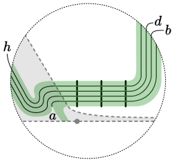
(a) Before truncation.

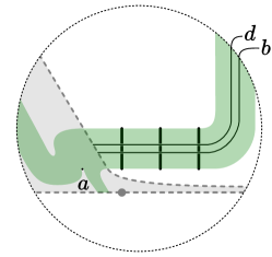
(b) First truncation.

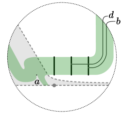
(c) Second truncation.

Figure 9.3. A magnification of the lower right of the toggle square in Figure 9.2. The routes $\eta$ (before truncation) are on the left. The routes $\eta^{\prime}$ (after first truncation) are in the centre. (The $\eta^{\prime}$ routes appear to end at points with different $x$--coordinate; this is an artefact of drawing the train-track with positive width.) The draping routes $\beta$ (after second truncation) are on the right.

Lemma 9.2.

The draping routes given in Definition 9.1 are well-defined.

Proof.

We must check in case (3) of Definition 9.1 that the end points of the draping routes lie inside of junctions. Moreover, we must also check that there is at least one more block free behind the endpoint. This is necessary because routes in the lower boundary of a crimped shearing region (but not in a toggle square) also appear in the upper boundary of the crimped shearing region immediately below, sheared back by one block.

We first fix notation. Suppose that $U$ is a crimped shearing region. Suppose that $H=\partial^{-}U$. Suppose that $k$ is a track-cusp of $\tau^{H}$. Consider the draping route $\beta(k)$.

Now suppose that we are in case (3a). Suppose that the endpoint of $\beta(k)$ lies in junction $J$ in the $m^{\rm th}$ block (as measured from the last block boundary as in Definition 8.13). By induction, $m$ is at most $w_{J}+2N$ where $N$ is the number of crimped shearing regions between $H$ and the toggle square meeting the upper boundary of $J$. Thus $N\leq h_{J}$. Since the number of blocks in $J$ is $w_{J}+2h_{J}$ we are done.

Instead, suppose that we are in case (3b). When we truncate $\eta(k)$, the end of $\eta^{\prime}(k)$ lands in a junction $J^{\prime}$, say. Suppose that to obtain $\beta(k)$ we truncate a segment of length $(n-1/2)b_{J^{\prime}}$ from the end of $\eta^{\prime}(k)$. The definition of $n$ ensures that there are no toggle squares in $H$ between the beginning and the end of $\beta(k)$. Let $K$ be the branch line containing $k$. Set $k_{0}=k$ and in general let $k_{i}$ be the intersection between $K$ and the lower boundary of the $i^{\rm th}$ crimped shearing region above $k$ as we travel up $K$. Let $\Sigma^{\prime}$ be the station containing $J^{\prime}$. The recursive construction of $\beta(k_{i})$ ensures that for $i\leq n$ there are no toggle squares intersecting $\eta(k_{i})$ between $k_{i}$ and $\Sigma^{\prime}$. Thus $n\leq w_{J^{\prime}}$. Since the number of blocks in $J^{\prime}$ is $w_{J^{\prime}}+2h_{J^{\prime}}$ we are done. See Figure 9.4. ∎

2pt $H$ [r] at 0 220 $k_{0}$ [r] at 170 220 $k_{1}$ [r] at 242 292 $k_{2}$ [r] at 314 364 $k_{3}$ [r] at 386 436 $J^{\prime}$ [l] at 764 148 $J^{\prime\prime}$ [l] at 620 148 $\Sigma^{\prime}$ [b] at 333 577

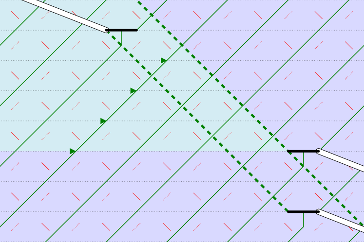
Figure 9.4. Straightened branch lines of $B^{\mathcal{V}}$, projected to the mid-surface $\mathcal{S}$. The station $\Sigma^{\prime}$ and the junctions $J^{\prime}$ and $J^{\prime\prime}$ are marked with dashed lines. In this example the height of $J^{\prime\prime}$ (and thus the width of $J^{\prime}$) is six. The cross-section $H$ and the cross-sections $k_{i}$ are also indicated. The draping route $\beta(k_{0})$ lies in $H$ and runs from $k_{0}$ to a point in the upper boundary of $J^{\prime}$. Note that $w_{J^{\prime}}$ only gives an upper bound for the number of track-cusps we must accommodate in $J^{\prime}\cap H$. The actual count is the number of branch lines in the green wedge that separate $J^{\prime}$ from any other toggle square in the wedge.

Definition 9.3.

Suppose that $k$ is a track-cusp in $B^{\mathcal{V}}\cap\partial^{-}\Theta_{\mathcal{V}}$. Let $\eta^{*}(k)$ be the route $\eta(k)$ (as in Definition 9.1) extended by $1/4$ of a block. ∎

Lemma 9.4.

The parting route $\alpha(k)$ is a subset of $\eta^{*}(k)$.

Proof.

Suppose that $\alpha(k)$ and $\eta^{*}(k)$ are contained in $\partial^{-}U$ where $U$ is a crimped shearing region. Both $\alpha(k)$ and $\eta(k)$ are created by folding routes in $\partial^{+}U$ downwards. The route creating $\alpha(k)$ has length zero and is the initial point of the route creating $\eta(k)$. The extra $1/4$ of a block is needed because we truncated a $3/4$ block to form $\alpha(k)$ but a full block to form $\eta(k)$. ∎

See Figures 9.1 and 9.2.

Lemma 9.5.

Suppose that $H$ is any cross-section. Suppose that $k$ and $\ell$ are track-cusps of $B^{\mathcal{V}}\cap H$. Then $\beta(k)$ and $\beta(\ell)$ do not cross (that is, there is a small motion of $\beta(k)$ making the two routes disjoint).

Furthermore, if $H$ is the lower boundary of a crimped shearing region $U$ then $\eta^{*}(k)$ and $\beta(\ell)$ do not cross.

Proof.

We use the notation of Definition 9.1. Let $[k_{0},k_{1}]$ and $[\ell_{0},\ell_{1}]$ be the resulting branch intervals in the branch lines $K$ and $L$ containing $k$ and $\ell$ respectively. Let $k_{r}$ and $\ell_{s}$ be the last points in these branch intervals for which there is a horizontal cross-section $H^{\prime}$ containing both. We deduce that $H^{\prime}$ is the upper boundary of some crimped shearing region $U$.

Claim 9.6.

$\beta(k_{r})$ and $\beta(\ell_{s})$ are disjoint, thus they do not cross.

Proof.

If $r=1$ then $\beta(k_{r})$ is contained in a station. In this case, if $\beta(\ell_{s})$ meets $\beta(k_{r})$ then (due to the truncation step of the construction) we find that $\beta(k_{r})=\beta(\ell_{s})$. Thus $k_{0}=\ell_{0}$ and we are done.

A similar proof deals with the case that $s=1$. We may now suppose that $r<1$ and $s<1$. Let $T^{\prime}$ be the union of the toggle squares of $H^{\prime}$. Define $H^{\prime\prime}=H^{\prime}-T^{\prime}$. Note that each component of $H^{\prime\prime}$ also appears as a subsurface of the lower boundary of some crimped shearing region. Since $k_{r}$ and $\ell_{s}$ are the last points of $[k_{0},k_{1}]$ and $[\ell_{0},\ell_{1}]$ in a common cross-section, we find that $k_{r}$ and $\ell_{s}$ are necessarily in different components of $H^{\prime\prime}$. By construction $\beta(k_{r})$ and $\beta(\ell_{s})$ are also contained in these components, so are disjoint.

Now suppose that $\eta^{*}(k)$ and $\beta(\ell)$ lie in the lower boundary of a crimped shearing region. By continuity $\eta(k)$ and $\eta(\ell)$ do not cross. Thus $\eta^{*}(k)$ and $\beta(\ell)$ do not cross. ∎

We now reparametrise $[k_{0},k_{r}]$ and $[\ell_{0},\ell_{s}]$ by the unit interval and re-choose our notation so that, for all $q\in[0,1]$, the track-cusps $k_{q}$ and $\ell_{q}$ lie in the same cross-section $H_{q}$. By the claim, when $q=1$ the routes $\beta(k_{q})$ and $\beta(\ell_{q})$ are disjoint in $H_{q}$. Let $\tau^{q}=B^{\mathcal{V}}\cap H_{q}$. The tracks $\tau^{q}$ fold as $q$ decreases. Folding preserves the property of not crossing, and we are done. ∎

9.2. The upper draping isotopy in $\Theta^{\mathcal{V}}$

In $\Theta^{\mathcal{V}}$, where $B^{\mathcal{V}}_{0}$ is almost a product, we perform (in time) an almost product splitting along the draping routes and then a lower graphical isotopy.

9.2.1. Splitting along draping routes

Suppose that $H$ is a horizontal cross-section in $\Theta^{\mathcal{V}}$ and suppose that $k\in B^{\mathcal{V}}\cap H$ is a track-cusp. Let $D$ be the difference between the $x$--coordinates of the beginning and end of $\beta(k)$. For $t\in[0,1/2]$ we split $k$ forward in a small neighbourhood of its draping route $\beta(k)$ at speed $2D$ (as measured in the $x$--coordinate).

Applying Lemma 9.5, when two track-cusps $k$ and $\ell$ meet, travelling in opposite directions, they split past each other. As they pass, they split to the left or right as determined by the combinatorics of their draping routes. Note that each track-cusp moves at the constant speed required for its journey to take all of $[0,1/2]$. Thus, by Lemma 9.5, track-cusps travelling in the same direction never meet.

This describes splitting along draping routes. The motion of the track-cusps, in an example, is shown in the lower three rows of Figure 9.5.

9.2.2. The graphical isotopy

All track-cusps of $B^{\mathcal{V}}_{1/2}\cap H$ lie in junctions. Also, by Lemmas 8.7 and 8.6, all branches of $B^{\mathcal{V}}_{1/2}\cap H$ are graphical with respect to the lower foliation.

So, for $t\in[1/2,1]$, we do the following. Outside of junctions we perform a lower graphical isotopy to make all branches straight in bigon coordinates. Due to our choice of radius of junctions (Definition 8.12) the straightened branches do not intersect junctions (other than the ones at their endpoints). Inside of junctions, the sidings remain fixed and other branches move so that their slopes (at the boundary) match the slopes outside of stations. See the upper three rows of Figure 9.5.

This describes the lower graphical isotopy.

2pt Graphical isotopy at 120 1000 Splitting along draping routes at 120 430

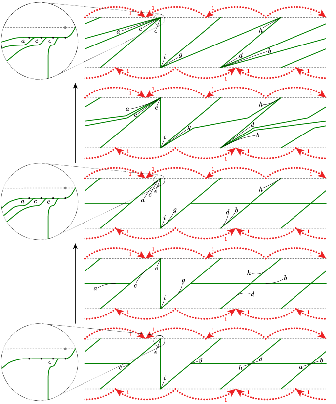
Figure 9.5. The draping isotopy for the cross-section $\partial^{-}\Theta^{\mathcal{V}}=\partial^{+}\Theta_{\mathcal{V}}$ at the middle of $U$. The five diagrams show (from the bottom moving up) $B^{\mathcal{V}}_{t}\cap H_{1/2}$ for $t\in(0,1/4,1/2,3/4,1)$. Here $U$ is the blue crimped solid torus for fLLQccecddehqrwjj_20102 . Following Definition 8.13 the number of blocks in the junction is eleven; however in each figure we only draw the blocks needed for the track-cusps in that figure.

Remark 9.7.

Suppose that $H$ is a cross-section in $\Theta^{\mathcal{V}}$. By construction (Definition 9.1) after splitting along draping routes and performing the lower graphical isotopy all track-cusps of $B^{\mathcal{V}}\cap H$ are in blocks in junctions.

As $H$ interpolates from $\partial^{-}\Theta^{U}$ to $\partial^{+}\Theta^{U}$, the only change in the train-tracks $B^{\mathcal{V}}\cap H$ is that track-cusps move forwards in their blocks. (Here we compare positions by projection in bigon coordinates.) ∎

Remark 9.8.

As in Remark 8.2, the intersection of the image of the upper draping isotopy with cross-sections in $\Theta^{\mathcal{V}}$ determines the intersection of the image of the upper draping isotopy with $\partial^{-}\Theta_{\mathcal{V}}$. For the result in our running example see Figure 9.6. ∎

2pt Graphical isotopy at -140 1030 Splitting along draping routes at -140 470

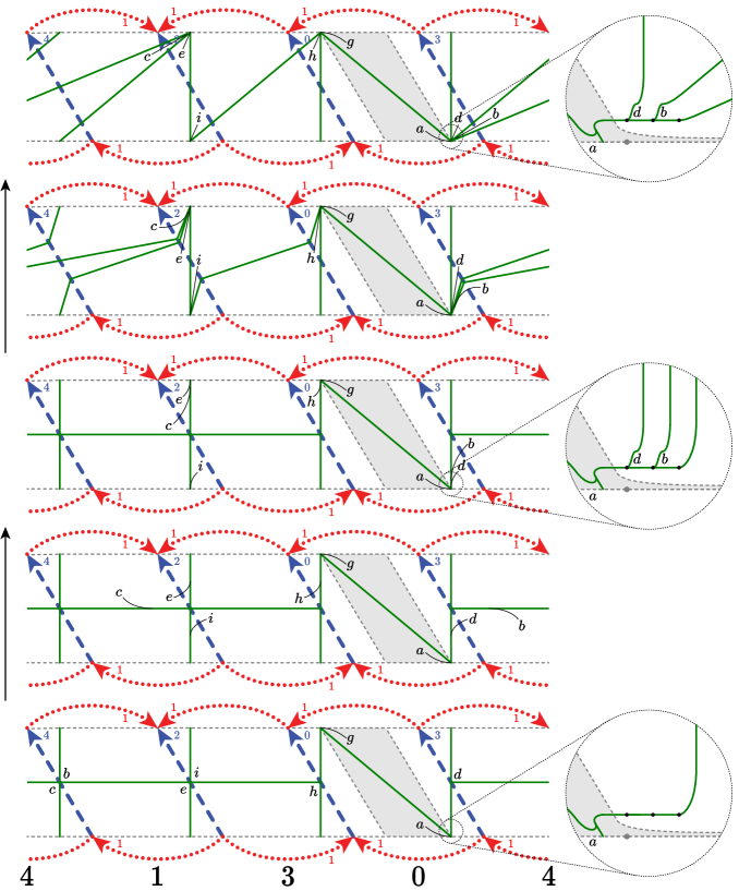
Figure 9.6. The draping isotopy for the cross-section $\partial^{-}\Theta_{U}$. The five diagrams show (from the bottom moving up) $B^{\mathcal{V}}_{t}\cap H_{0}$ for $t\in(0,1/4,1/2,3/4,1)$. Here $U$ is the blue crimped solid torus for fLLQccecddehqrwjj_20102 .

9.3. The upper draping isotopy in $\Theta_{\mathcal{V}}$

Fix $U$, a blue crimped shearing region. We use $H_{s}$ to denote the cross-section of $\Theta_{U}$ at height $s\in[0,1/2]$. It remains to describe the intersections $B^{\mathcal{V}}_{t}\cap H_{s}$. The intersections $B^{\mathcal{V}}_{0}\cap H_{s}$ are given by parted position. Also, $B^{\mathcal{V}}_{t}\cap H_{1/2}$ and (by Remark 9.8) $B^{\mathcal{V}}_{t}\cap H_{0}$ are determined by the splitting and lower graphical isotopy given in Section 9.2. This gives three sides of the boundary of the isotopy.

9.3.1. Suffix routes

We now describe the fourth side; that is, we describe $B^{\mathcal{V}}_{1}\cap H_{s}$ for $s\in[0,1/2]$. To do this we start from the given $B^{\mathcal{V}}_{1}\cap H_{0}$ and perform (in space):

• a splitting along suffix routes to produce $B^{\mathcal{V}}_{1}\cap H_{1/4}$ followed by

• a lower graphical isotopy to $B^{\mathcal{V}}_{1}\cap H_{1/2}$.

Definition 9.9.

Suppose that $k_{0,0}$ is a track-cusp of $B^{\mathcal{V}}_{0}\cap H_{0}$. We take $\beta(k_{0,0})$ as given by Definition 9.1. We take $\eta^{*}(k_{0,0})$ as given by Definition 9.3. We define $\gamma^{*}=\eta^{*}(k_{0,0})-\beta(k_{0,0})$. This is well-defined because $\beta(k_{0,0})\subset\eta(k_{0,0})$.

Let $k_{1,0}$ be the track-cusp of $B^{\mathcal{V}}_{1}\cap H_{0}$ which is the endpoint of $\beta(k_{0,0})$. By Lemma 9.5 none of the draping routes in $B^{\mathcal{V}}_{0}\cap H_{0}$ cross $\gamma^{*}$. Therefore we may define $\gamma(k_{1,0})$, the suffix route for $k_{1,0}$, by taking the image of $\gamma^{*}$ under the splitting and lower graphical isotopy defined in Section 9.2. Note that $\gamma(k_{1,0})$ starts at $k_{1,0}$ and is carried by $B^{\mathcal{V}}_{1}\cap H_{0}$. ∎

As in Sections 8.5 and 9.2.1, we now perform a splitting (in space) along the suffix routes $\gamma$. As $s$ progresses through $[0,1/2]$ we split each track-cusp $k_{1,0}$ forward along its suffix route $\gamma(k_{1,0})$.

With that done, we perform (in space) a lower graphical isotopy, analogous to the ones described in Sections 8.6 and 9.2.2. As $s$ progresses through $[1/4,1/2]$, outside of junctions we straighten the train-track by a graphical isotopy along the lower foliation. Since this is an isotopy in space, just as in Section 8.6, inside of junctions track-cusps move forward to maintain dynamism (at constant speed within their blocks) and branches move via graphical isotopy along the lower foliation as needed. See Figure 9.7.

2pt Graphical isotopy at 110 1040 Splitting along suffix routes at 110 470 $\partial^{+}\Theta_{U}$ [r] at -20 1337 $\partial^{-}\Theta_{U}$ [r] at -20 179

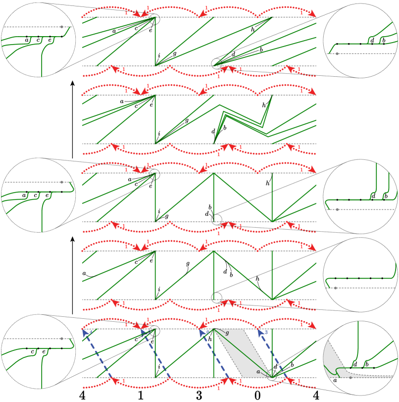
Figure 9.7. The result $B^{\mathcal{V}}_{1}$ of the draping isotopy in $\Theta_{U}$ where $U$ is the blue crimped solid torus for fLLQccecddehqrwjj_20102 . The five diagrams show (from the bottom moving up) $B^{\mathcal{V}}_{1}\cap H_{s}$ for $s\in(0,1/8,1/4,3/8,1/2)$.

9.3.2. Prefix routes

Now that we have constructed the four sides of the isotopy we fill in the interior. That is, we describe the train-tracks $B^{\mathcal{V}}_{t}\cap H_{s}$ for $s\in(0,1/2)$ and $t\in(0,1)$. To build $B^{\mathcal{V}}_{t}\cap H_{s}$ we start from $B^{\mathcal{V}}_{0}\cap H_{s}$ and perform (in time)

• a splitting along prefix routes to produce $B^{\mathcal{V}}_{1/2}\cap H_{s}$ followed by

• a lower graphical isotopy to $B^{\mathcal{V}}_{1}\cap H_{s}$.

Notation 9.10.

Where defined, we take $k_{t,s}$ to be the track-cusp of $B^{\mathcal{V}}_{t}\cap H_{s}$ corresponding to $k_{0,0}$. Let $x_{t,s}$ be the $x$–coordinate of $k_{t,s}$ (in bigon coordinates). ∎

Remark 9.11.

Suppose that $s$ lies in $(0,1/2)$. Suppose that $J$ is the junction containing the endpoint of $\beta(k_{0,s})$. Breaking symmetry, suppose that the orientation of $\beta(k_{0,0})$ points in the direction of increasing $x$–coordinate. Thus the same holds for the orientation of $\beta(k_{0,s})$. With the above notation, the endpoints of $\beta(k_{0,s})$ have $x$–coordinates

$$x_{0,s}\quad\mbox{and}\quad x_{1,1/2}-(1/2-s)b_{J}$$

where $b_{J}$ is the block length defined in Definition 8.13. ∎

Definition 9.12.

Suppose that $s$ lies in $(0,1/2)$. We define the prefix route $\delta(k_{0,s})$ to be the prefix of $\beta(k_{0,s})$ which ends at the point with $x$–coordinate equal to $x_{1,s}$. ∎

Lemma 9.13.

With the above notation, for all $s\in(0,1/2)$ we have

$$x_{0,s}\leq x_{1,s}\leq x_{1,1/2}-(1/2-s)b_{J}$$

Thus the coordinate $x_{1,s}$ lies in the interval of $x$–coordinates of the draping route $\beta(k_{0,s})$. Thus the prefix route $\delta(k_{0,s})$ is well-defined.

Proof.

Again breaking symmetry, suppose that the orientation of $\beta(k_{0,0})$ points in the direction of increasing $x$–coordinate. It follows that the same holds for $\alpha(k_{0,0})$ and $\gamma(k_{1,0})$. The lengths of the various routes, the motion of track-cusps during graphical isotopies, and Lemma 9.4 give the inequalities shown in Table 9.1. (The ordering of $x_{1,0}$ and $x_{0,1/2}$ depends on the combinatorial type of the track-cusp $k_{0,0}$.)

$x_{0,1/2}$	$\leq$	$x_{1,1/2}$
$<$		$<$
$x_{0,1/4}$	$\leq$	$x_{1,1/4}$
$<$		$<$
$x_{0,0}$	$\leq$	$x_{1,0}$

Table 9.1.

We now show that $x_{0,s}\leq x_{1,s}$. Suppose that $s$ lies in $(0,1/4)$. Note that $x_{0,s}$ is a barycentric combination of $x_{0,0}$ and $x_{0,1/4}$. Likewise $x_{1,s}$ is a barycentric combination of $x_{1,0}$ and $x_{1,1/4}$, with the same coefficients. Thus the first inequality follows from the middle and lower lines of Table 9.1. The same argument, applied to the upper and middle lines of Table 9.1, deals with $s$ lying in $(1/4,1/2)$.

We now show that $x_{1,s}\leq x_{1,1/2}-(1/2-s)b_{J}$. Suppose that $s$ lies in $(1/4,1/2)$. The track-cusp $k_{1,s}$ is in its block and moving at speed exactly $b_{J}$. Note that $x_{1,1/2}-(1/2-s)b_{J}$ also moves at speed exactly $b_{J}$. This establishes the inequality (in fact equality) for $s$ in $(1/4,1/2)$. Now suppose that $s$ lies in $(0,1/4)$. By construction $\gamma(k_{1,0})$ has length at least $\frac{1}{4}b_{J}$, so $x_{1,s}$ moves at speed at least $b_{J}$. Thus the inequality also holds for $s$ in $(0,1/4)$. ∎

For each fixed $s$ in $(0,1/2)$, we split along the prefix routes (for $t\in[0,1/2]$). While splitting, each track-cusp moves from its position in $B^{\mathcal{V}}_{0}\cap H_{s}$ to its position in $B^{\mathcal{V}}_{1}\cap H_{s}$. We then perform the lower graphical isotopy (for $t\in[1/2,1]$); since this is an isotopy in time rather than space, the track-cusps do not move.

This completes the definition of the upper draping isotopy; we call the result draped position. Note that the upper draping isotopy is continuous by construction.

The lower draping isotopy of $B_{\mathcal{V}}$ is defined analogously, with the roles of $\Theta^{U}$ and $\Theta_{U}$ reversed. For examples, see Figures 9.8, 9.9, and 9.10.

9.4. Draped position

With draped position in hand we make a sequence of observations.

2pt $\partial^{+}\Theta^{\mathcal{V}}$ [r] at 10 835 $\partial^{-}\Theta^{\mathcal{V}}=\partial^{+}\Theta_{\mathcal{V}}$ [r] at 10 505 $\partial^{-}\Theta_{\mathcal{V}}$ [r] at 10 185

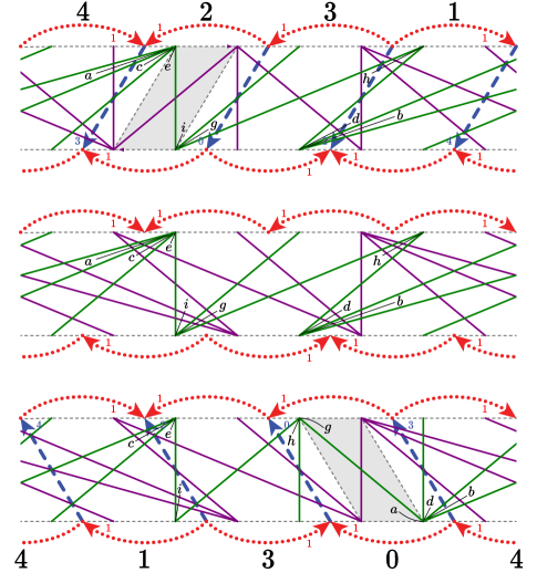
(a) Blue crimped solid torus.

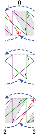
(b) Red.

Figure 9.8. The intersection of $B^{\mathcal{V}}$ (and $B_{\mathcal{V}}$), in draped position, with various cross-sections ($s=0,1/2,1$) of the crimped shearing decomposition of fLLQccecddehqrwjj_20102 . Compare with Figure 8.1.

2pt $\partial^{+}\Theta^{\mathcal{V}}$ [r] at 10 780 $\partial^{-}\Theta^{\mathcal{V}}=\partial^{+}\Theta_{\mathcal{V}}$ [r] at 10 450 $\partial^{-}\Theta_{\mathcal{V}}$ [r] at 10 130 a at 120 845 c at 120 780 d at 65 790 b at 65 735

a at 145 490 d at 70 500 d at 220 500 b at 245 425 b at 45 425 c at 110 415 c at 180 415

a at 170 195 c at 170 130 d at 225 140 b at 225 75

Remark 9.14.

Suppose that $H$ is any cross-section. Suppose that $J$ is a junction which intersects $H$. Suppose that $B^{\mathcal{V}}$ is in draped position. Let $b$ be a branch of either $\tau^{H}$ or $\tau_{H}$. By our choice of radius $r_{J}$ (Definition 8.12), the branch $b$ intersects $J$ if and only if (at least) one end of $b$ lies in $J$. ∎

Lemma 9.15.

In draped position, the branched surfaces $B^{\mathcal{V}}$ and $B_{\mathcal{V}}$ are dynamic.

Proof.

In draped position the branched surface $B^{\mathcal{V}}$ is transverse to the cross-sections of all crimped shearing regions. Furthermore, we have arranged that track-cusps always move forwards as we move up through cross-sections. The same argument applies to $B_{\mathcal{V}}$. ∎

Suppose that $H$ is a cross-section in a crimped shearing region $U$. Suppose that $B^{\mathcal{V}}$ and $B_{\mathcal{V}}$ are in draped position. We again define $\tau^{H}=B^{\mathcal{V}}\cap H$ and $\tau_{H}=B_{\mathcal{V}}\cap H$.

Remark 9.16.

Suppose that $B^{\mathcal{V}}$ and $B_{\mathcal{V}}$ are in draped position. Suppose that $U$ is a crimped shearing region. Suppose that $H$ is either $\partial^{+}U$, the upper boundary of $U$, or $\partial^{-}U$, the lower boundary.

1. Each track-cusp of $\tau^{H}$ and $\tau_{H}$ is in a junction.

2. Outside of the junctions, the branches of $\tau^{H}$ and $\tau_{H}$ are line segments (in bigon coordinates).

3. Suppose that $e$ is a helical edge in $H$. Suppose that, of the two equatorial squares adjacent to $e$, at least one contains a toggle square. Then the upper junctions immediately adjacent to $e$ are connected by a branch of $\tau^{H}$. Similarly, the lower junctions are connected by a branch of $\tau_{H}$.

4. Every component of $H-\tau^{H}$ contains exactly one track-cusp, and exactly one ideal vertex of $U$. The same holds for $H-\tau_{H}$.

Moreover, if $U$ is a blue shearing region then we have the following.

1. Outside of toggle squares and junctions, the branches of $\tau^{H}$ have strictly positive slope (in bigon coordinates on $H$) and the branches of $\tau_{H}$ have strictly negative slope.

2. Inside of toggle squares, outside of junctions, there is exactly one branch of $\tau^{H}$ and exactly one branch of $\tau_{H}$. If $H=\partial^{+}U$ then these branches have strictly positive slope with the slope of $\tau^{H}$ more positive than that of $\tau_{H}$. If instead $H=\partial^{-}U$ then these branches have strictly negative slope with the slope of $\tau_{H}$ more negative than that of $\tau^{H}$.

When $U$ is a red shearing region, similar statements hold, swapping the signs of slopes. ∎

In our figures, some branches of the draped train-tracks appear to be vertical, contradicting Remark 9.16(5) and (6). However, due to the perturbation of Remark 6.1(3) and our choice of junction radius (Definition 8.12), these branches in fact have finite slopes.

We generalise Remark 9.16(4) to other cross-sections as follows.

Proposition 9.17.

Suppose that $U$ is a crimped shearing region. Let $H$ be a cross-section of $U$. Then every component of $H-\tau^{H}$ contains exactly one track-cusp and exactly one ideal vertex of $U$. The same holds for $H-\tau_{H}$.

Proof.

The result holds for $H^{\prime}=\partial^{-}U$ by Remark 9.16(4). Moving upwards from $H^{\prime}$ to $H$ we perform splittings and graphical isotopies. Neither of these changes the combinatorics of a region of $H-\tau^{H}$. ∎

From Remarks 9.7 and 9.16 we deduce the following.

Corollary 9.18.

Suppose that $B^{\mathcal{V}}$ and $B_{\mathcal{V}}$ are in draped position. Suppose that $U$ is a blue shearing region. Suppose that $H$ is the lower boundary of $\Theta^{U}$ (which equals the upper boundary of $\Theta_{U}$).

1. Each track-cusp of $\tau^{H}$ and $\tau_{H}$ is in a junction.

2. Outside of the junctions, the branches of $\tau^{H}$ and $\tau_{H}$ are line segments (in bigon coordinates).

3. Outside of the junctions, the branches of $\tau^{H}$ have strictly positive slope and the branches of $\tau_{H}$ have strictly negative slope.

Finally, all of the above again holds, swapping slopes appropriately, when $U$ is a red shearing region. ∎

Lemma 9.19.

Suppose that $B^{\mathcal{V}}$ and $B_{\mathcal{V}}$ are in draped position. Suppose that $U$ is a blue shearing region. Suppose that $H$ is any cross-section of $U$. Let $c$ be a cusp of $U$. Let $E$ be the component of $H-(\tau^{H}\cup\tau_{H})$ meeting $c$. Then (outside of junctions) the branches of $\tau^{H}$ appearing in the boundary of $E$ have positive slope; the branches of $\tau_{H}$ appearing in the boundary of $E$ have negative slope. There is a similar statement for a red shearing region.

Proof.

We begin by considering branches of the upper train-track in $\partial^{-}U$. By Remark 9.16(5) and (6), the only branches of the incorrect slope are in toggle squares. Appealing to Remark 9.16(3), such branches are separated from the cusp $c$ by other branches.

We now move upwards from $\partial^{-}U=\partial^{-}\Theta_{U}$ to $\partial^{+}\Theta_{U}$. Splitting along draping routes does not change the slopes of branches appearing in the boundary of $E$. The graphical isotopy does change slopes. Positive slopes remain positive, while any negative slopes (above toggle squares) become positive. Moreover, branches with negative slope never make up part of the boundary of $E$ because the graphical isotopies follow the lower foliation. ∎

Lemma 9.20.

Each subray of each branch line of $B^{\mathcal{V}}$ and of $B_{\mathcal{V}}$, in draped position, meets crimped shearing regions of both colours.

Proof.

This follows from Lemma 2.2 and the fact that our isotopies do not change combinatorics in toggle squares. ∎

10. The dynamic pair

Theorem 10.1.

Suppose that $\mathcal{V}$ is a transverse veering triangulation. In draped position, the upper and lower branched surfaces $B^{\mathcal{V}}$ and $B_{\mathcal{V}}$ form a dynamic pair; this position is canonical. Furthermore, if $\mathcal{V}$ is finite then draped position is produced algorithmically in polynomial time. Finally, the dynamic train-track $B^{\mathcal{V}}\cap B_{\mathcal{V}}$ has at most a quadratic number of edges.

The branched surfaces $B^{\mathcal{V}}$ and $B_{\mathcal{V}}$ are individually dynamic by Lemma 9.15. We now verify the hypotheses of Definition 4.7. Again, it will be convenient to work equivariantly in the universal cover.

10.1. Transversality

Let $U$ be a crimped shearing region.

Lemma 10.2.

Suppose that $H$ is a cross-section of $U$. Then the train-tracks $\tau^{H}$ and $\tau_{H}$ are transverse.

Proof.

Let $H_{s}$, for $s\in[0,1/2]$, be the cross-sections of $\Theta_{U}$. Let $\tau^{s}=B^{\mathcal{V}}\cap H_{s}$ and let $\tau_{s}=B_{\mathcal{V}}\cap H_{s}$. The train-tracks $\tau^{0}$ and $\tau_{0}$ are transverse by Remark 9.16(1), (5), and (6), as well as Remark 9.14. As $s$ increases, the train-tracks $\tau^{s}$ perform the neighbourhood and then graphical isotopies as described in Section 9.3. Also, by Remark 9.7, the train-tracks $\tau_{s}$ are all essentially the same in bigon coordinates.

During the splitting (that is, for $s\in[0,1/4]$), the track-cusps of $\tau^{s}$ split forward in a small neighbourhood of (the projection of) $\tau^{0}$. Thus the train-tracks $\tau^{s}$ and $\tau_{s}$ are transverse for $s\in[0,1/4]$.

By Corollary 9.18, the train-tracks $\tau^{1/2}$ and $\tau_{1/2}$ are transverse. We now consider $s\in[1/4,1/2]$. The graphical isotopy interpolates between $\tau^{1/4}$ and $\tau^{1/2}$. Let $b^{s}$ and $c_{s}$ be branches of $\tau^{s}$ and $\tau_{s}$ respectively.

Claim.

The branches $b^{s}$ and $c_{s}$ are transverse.

Proof.

By Remark 9.7, in $\Theta_{U}$ the track-cusps of $\tau_{H}$ lie within junctions. The lower graphical isotopy leaves upper track-cusps in junctions, and the upper and lower junctions are disjoint. Thus the endpoints of $b^{s}$ and $c_{s}$ are disjoint.

Let $c_{0}$ be the projection of $c_{s}$ down to $\partial^{-}U$. Suppose that $c_{0}$ lies completely within a toggle square. If the projection of $b^{1/2}$ misses this toggle square then we are done. Otherwise let $a^{s}$ be the linear segment of $b^{s}$ whose projection meets the toggle square. Since the isotopy is lower graphical, the slope of $a^{s}$ is between that of $a^{1/4}$ and $a^{1/2}$. Applying Remark 9.16(6) and Corollary 9.18(3) we find that the slope of $c_{s}$ is more negative than that of $a^{s}$. We deduce that $c_{s}$ is transverse to $a^{s}$ and thus to $b^{s}$.

Suppose instead that $c_{0}$ is disjoint from the toggle squares. In this case the proof is similar, but easier. Now the slope of $c_{s}$ is always negative by Corollary 9.18(3). Also, the slope of $a^{s}$ is always positive by Remark 9.16(5), by Corollary 9.18(3), and by appealing to the lower graphical isotopy. ∎

Swapping the roles of upper and lower and repeating the argument shows that $\tau^{H}$ and $\tau_{H}$ are transverse for every cross-section $H$ in $\Theta^{U}$. ∎

This lemma proves that $B^{\mathcal{V}}$ and $B_{\mathcal{V}}$ are transverse. The proof above also implies the following.

Remark 10.3.

As $H$ moves upwards, if a track-cusp of $\tau^{H}$ moves through $\tau_{H}$, it does so going forwards. Similarly, whenever a track-cusp of $\tau_{H}$ moves through $\tau^{H}$, it does so going backwards. ∎

10.2. Components

We must show that every component $C$ of $M-(B^{\mathcal{V}}\cup B_{\mathcal{V}})$ is either a dynamic shell (Definition 4.4) or a pinched tetrahedron (Definition 4.1).

10.2.1. Dynamic shell

Suppose that $C$ contains one (thus by Proposition 9.17, exactly one) cusp $c$ of $M$. Let $v$ be a model of $c$ where $v$ is an ideal vertex of a red crimped shearing region $U$. Let $E=E(v,U)$ be the component of $U-(B^{\mathcal{V}}\cup B_{\mathcal{V}})$ incident to $v$. Our goal now is to prove the following.

• $E$ is a three-ball,

• the frontier of $E$ in $U$ consists of two vertical ‘‘half-bigons’’ (one from each of $B^{\mathcal{V}}$ and $B_{\mathcal{V}}$),

• the boundary of $E$ in $\partial^{+}{U}$ consists of a triangle, intersecting a single helical edge of $\partial^{+}U$, and

• the boundary of $E$ in $\partial^{-}{U}$ consists of a triangle, intersecting a single helical edge of $\partial^{-}U$.

Fix a cross-section $H$ of $U$. Looking into $H$ from the vertex $v$, we see a branch of $\tau_{H}$ ending on the boundary of $H$ to our left and a branch of $\tau^{H}$ ending on the boundary of $H$ to our right. Appealing to Lemma 9.19, the frontier of $H\cap E$ lies in a train route of $\tau^{H}$ and a train route of $\tau_{H}$. For each $H$, these routes intersect precisely once. Stacking the cross-sections together, the routes form the desired half-bigons. This shows that $E$ is a three-ball with the desired properties.

A similar argument applies for a blue shearing region $U$. Here the half-bigon of $B^{\mathcal{V}}$ is to the left, and the half-bigon of $B_{\mathcal{V}}$ is to the right.

Taking the union of the three-balls $E(v,U)$, as $v$ ranges over the models of $c$, gives $C$. The half-bigons glue to give the stable and unstable faces of $C$. Note that any one half-bigon meets only finitely many others because the edges of $\mathcal{V}$ have finite degrees. Therefore, the $E(v,U)$ glue together to form a dynamic shell.

10.2.2. Pinched tetrahedron

Before obtaining our pinched tetrahedra we need the following definition and lemma.

Definition 10.4.

Suppose that $H\subset U$ is a cross-section. We define the bigon extension $\stackon[1pt]{H}{\kern 3.20007pt\scalebox{0.6}{\rotatebox{90.0}{$\llparenthesis$} }}$ as follows. The boundary of $H$ consists of longitudinal crimped edges. Each such edge $e$ cobounds a crimped bigon $B$ with a veering edge $e^{\prime}$. We obtain $\stackon[1pt]{H}{\kern 3.20007pt\scalebox{0.6}{\rotatebox{90.0}{$\llparenthesis$} }}$ by gluing each such crimped bigon $B$ to $H$ along its edge $e$. ∎

We now suppose that $C$ is a component of $M-(B^{\mathcal{V}}\cup B_{\mathcal{V}})$ which does not contain any cusp $c$ of $M$.

Lemma 10.5.

Suppose that $H$ is a cross-section of a crimped shearing region $U$, meeting $C$. Then the intersection $C\cap\stackon[1pt]{H}{\kern 3.20007pt\scalebox{0.6}{\rotatebox{90.0}{$\llparenthesis$} }}$ is either a trigon or a quadragon, as defined in Definition 4.3. Moreover, as $H$ moves up through $U$, components change according to the sequence given in Definition 4.3.

Proof.

Suppose that $U$ is a red crimped shearing region. Let $H_{s}$ for $s\in[0,1]$ be the cross-sections of $U$. Thus $H_{0}=\partial^{-}U$.

Claim.

Let $\textsc{r}=C\cap\stackon[1pt]{H}{\kern 3.20007pt\scalebox{0.6}{\rotatebox{90.0}{$\llparenthesis$} }}_{0}$. Then r is either a trigon or a quadragon.

Proof.

First suppose that r is entirely contained within $H=H_{0}$. Appealing to Remark 9.16, the boundary of r is a piecewise loop in $H$ with either three or four corners. (Outside of toggle squares, the two train-tracks have opposite signs so there cannot be more than four corners. Inside of toggle squares the combinatorics is standardised.) These corners are either at transverse intersections between $\tau^{H}$ and $\tau_{H}$ or at track-cusps. If there are four corners then they are all transverse intersections between $\tau^{H}$ and $\tau_{H}$ and r is a quadragon. If there are three corners then two are transverse intersections and one is a track-cusp. Thus r is a trigon.

Now suppose that r is not entirely contained within $H$. By Remark 9.16(3), the component r meets a crimped bigon $B$ and contains the midpoint of the crimped edge. The frontier of r in $B$ consists of exactly one arc from each of $\tau^{B}$ and $\tau_{B}$, meeting at a point. The claim now follows in a manner similar to the previous paragraph. ∎

More generally, suppose that the claim holds with $H_{s}$ replacing $H_{0}$. Let $\tau^{s}=H_{s}\cap B^{\mathcal{V}}$ (green) and $\tau_{s}=H_{s}\cap B_{\mathcal{V}}$ (purple). Remark 10.3 tells us that as $s$ increases, there are only two combinatorial changes:

1. Track-cusps of $\tau^{s}$ move forwards through branches of $\tau_{s}$.

2. Track-cusps of $\tau_{s}$ move backwards through branches of $\tau^{s}$.

The first move simultaneously creates a new green trigon and converts a green trigon into a quadragon. The second move simultaneously deletes a purple trigon, and converts a quadragon into a purple trigon. These are both moves between stages in the life of a pinched tetrahedron, as given in Definition 4.3, as required. This proves Lemma 10.5. ∎

Equipped with this lemma we now prove that $C$ is a pinched tetrahedron. Let $H$ be a cross-section through a crimped shearing region $U$. Let r be a region of $\stackon[1pt]{H}{\kern 3.20007pt\scalebox{0.6}{\rotatebox{90.0}{$\llparenthesis$} }}-(B^{\mathcal{V}}\cup B_{\mathcal{V}})$. Let $S^{\textsc{r}}$ be the component of $\stackon[1pt]{H}{\kern 3.20007pt\scalebox{0.6}{\rotatebox{90.0}{$\llparenthesis$} }}-\tau^{H}$ containing r. Let $S_{\textsc{r}}$ be the component of $\stackon[1pt]{H}{\kern 3.20007pt\scalebox{0.6}{\rotatebox{90.0}{$\llparenthesis$} }}-\tau_{H}$ containing r. Thus $\textsc{r}=S_{\textsc{r}}\cap S_{\textsc{r}}$. Using Proposition 9.17 twice, gives a pair of track-cusps $s^{\textsc{r}}\subset S^{\textsc{r}}$ and $s_{\textsc{r}}\subset S_{\textsc{r}}$.

First suppose that r is a green trigon. Thus r contains $s^{\textsc{r}}$. We must show that this track-cusp eventually crosses a purple arc, turning r into a quadragon. By Lemma 9.20, moving up, (the branch line containing) $s^{\textsc{r}}$ eventually enters the bottom of a crimped shearing region $V$ through a toggle square. If the region r persists into $\partial^{-}V$, and is still a green trigon, then moving up through $\Theta_{V}$, the track-cusp $s^{\textsc{r}}$ splits forwards and hits the purple arc given by Remark 9.16(3). This turns r into a quadragon.

Moving down instead of up, a similar argument shows that every green trigon is born at some point. Similar arguments also show that as we move up purple trigons eventually die, and that as we move down, purple trigons eventually turn into quadragons.

Lastly we must show that no quadragon can remain a quadragon forever. Suppose now that r is a quadragon in a cross-section $H$. As we move down, (the branch line containing) $s^{\textsc{r}}$ is eventually inside a toggle square within a cross-section $K=\partial^{-}U$. Using Remark 9.16(3), we observe that the component of $\stackon[1pt]{K}{\kern 3.20007pt\scalebox{0.6}{\rotatebox{90.0}{$\llparenthesis$} }}-B^{\mathcal{V}}$ containing $s^{\textsc{r}}$ has no quadragons. Therefore for some cross-section below $H$ and above $K$, the region r became a trigon. A similar argument shows that quadragons must eventually become trigons as we move upwards.

This completes the proof that components of $M-(B^{\mathcal{V}}\cup B_{\mathcal{V}})$ are either dynamic shells or pinched tetrahedra.

10.3. Transience

Suppose that $F$ is a component of $B_{\mathcal{V}}-B^{\mathcal{V}}$. Let $\alpha$ be an upwards ray in $F$, in the sense of Definition 4.6. Let $x$ be the initial point of $\alpha$. Let $U$ be a crimped shearing region containing $x$, and let $H$ be the cross-section of $U$ containing $x$. Proposition 9.17 implies that there is one ideal vertex $v$ of $U$ in the component of $H-\tau^{H}$ containing $x$. Let $c$ be the cusp of $M$ containing $v$. By Section 10.2, there is a unique dynamic shell $C$ containing $c$.

Let $(\textsc{r}_{i})$ be the (necessarily finite) collection of components of $H-(\tau^{H}\cup\tau_{H})$ which separate, in $H-\tau^{H}$, the region $C\cap H$ from the point $x$. Let $f\subset F\cap H$ be the component containing $x$. As we flow upwards through cross-sections $H_{s}$, even when we move from one crimped shearing region to the next, each of the $\textsc{r}_{i}$ evolves according to Definition 4.3. Thus they all eventually collapse. Moreover, by Remark 10.3, no new regions are created between $\alpha\cap H_{s}$ and $C\cap H_{s}$. So $\alpha$ eventually flows into an unstable face of $C$. The same argument applies to components of $B^{\mathcal{V}}-B_{\mathcal{V}}$, flowing downwards.

10.4. Separation

Recall from Remark 2.1 that both $B^{\mathcal{V}}$ and $B_{\mathcal{V}}$ are isotopic (ignoring the branching structure) to the dual two-skeleton of $\mathcal{V}$. Suppose that $C$ and $D$ are components of $M-(B^{\mathcal{V}}\cup B_{\mathcal{V}})$, each containing a cusp of $M$. Thus, by Proposition 9.17, each of $C$ and $D$ contains exactly one cusp of $M$. Suppose that $F$ is a two-cell of the natural cell structure on $B^{\mathcal{V}}\cup B_{\mathcal{V}}$. Suppose that $F$ meets $C$ on one side and $D$ on the other. Then we can find a proper arc dual to $F$, and thus disjoint from one of $B^{\mathcal{V}}$ or $B_{\mathcal{V}}$. This is a contradiction.

10.5. Canonicity and complexity

The construction does not make any arbitrary choices so draped position is canonical. In particular, if we reverse the orientation of the manifold or the coorientation of the faces of the triangulation (or both) then only labels change; the underlying combinatorics of the dynamic pair remains the same.

Now suppose that $\mathcal{V}$ is a finite transverse veering triangulation. Let $|\mathcal{V}|$ denote the number of veering tetrahedra. In building the shearing decomposition (Theorem 5.6), we produce $2|\mathcal{V}|$ half-tetrahedra and perform $2|\mathcal{V}|$ gluings. This requires linear time. In producing the crimped shearing decomposition (Section 5.2), the work is now proportional to the sum of the edge degrees, which is $6|\mathcal{V}|$. This again requires linear time.

To specify the draped positions of $B^{\mathcal{V}}$ and $B_{\mathcal{V}}$, it suffices to determine the position of every track-cusp $c$ in each horizontal cross-section $H$ appearing in the $\Theta$--decomposition of every crimped shearing region $U$. The branch intervals of $B^{U}$ lie in junctions except, possibly, in the lower half of $\Theta_{U}$. Taking $H=\partial^{-}U$, and supposing that the track-cusp $c$ lies in a toggle square, we find that $c$ splits forward in the (space) splitting described in Section 9.3. The path of $c$ is exactly the train route $\beta(c)$ described in Section 9.2. The naive algorithm to produce the route takes time at most quadratic in the heights and widths of various junctions. Thus the total time required to compute the $\beta$ routes is polynomial.

We now bound the number of edges in the dynamic train-track $B^{\mathcal{V}}\cap B_{\mathcal{V}}$. Note that the dynamic train-track is disjoint from the junctions (Remark 9.14). Suppose that $(U_{i})_{i=1}^{m}$ is a collection of blue crimped shearing regions with the following properties.

1. $U=U_{1}$ has at least one toggle square in $\partial^{-}U$.

2. $V=U_{m}$ has at least one toggle square in $\partial^{+}V$.

3. For $i=1,2,\ldots,m-1$, the upper boundary of $U_{i}$ equals the lower boundary of $U_{i+1}$.

4. There are no toggle squares in this shared cross-section.

5. The length of $U$, and thus of all of the $U_{i}$, is $n$.

We allow $m$ to be one (and thus $U=V$). We also allow $n$ to be one.

Let $H=\partial^{+}\Theta_{U}$ be the middle cross-section of $U$. The track $\tau_{H}$ has $2n$ branches (outside of the junctions). Each of these branches is a line segment in $H$. Since the draping isotopy is fixed on toggle squares, consulting Figure 8.3d and recalling Remark 9.7, each branch of $\tau_{H}$ above a toggle square has projection to $\partial^{-}U$ contained within that toggle square. The remaining branches of $\tau_{H}$ have projections that avoid the toggle squares. Thus no branch of $\tau_{H}$ wraps all the way around $H$. Thus their slopes are more negative than $-1/n$ (times a universal factor of $\sqrt{3}/2$, which we ignore).

Let $K=\partial^{-}\Theta^{V}$ be the middle cross-section of $V$. By a similar argument, $\tau^{K}$ has $2n$ branches (outside of the junctions). Again, each is a line segment in $K$. Furthermore, all of these are either below toggle squares or have slope greater than $1/n$. Since there are no toggle squares between $U$ and $V$ the track $\tau^{H}$ is obtained from $\tau^{K}$ by shearing one unit, $m$ times. Thus the branches of $\tau^{H}$ have slope greater than $1/(m+n)$. Therefore any branch of $\tau^{H}$ wraps at most $(m+n)/n$ times around $H$. It follows that each branch of $\tau^{H}$ meets each branch of $\tau_{H}$ at most $((m+n)/n)+1$ times. There are $(2n)^{2}$ such pairs, for a total of at most $4n(m+2n)$ intersections. This counts all edges of the dynamic train-track above $H$ and below $K$. Edges of the dynamic train-track either continue or merge in pairs as we descend from $H$ to $\partial^{-}U$. Thus there are at most an additional $4n(m+2n)$ edges in $\Theta_{U}$. Likewise there are at most an additional $4n(m+2n)$ edges in $\Theta^{V}$.

There are now two cases. If $m\geq n$ then the size of the dynamic train-track in $\cup_{i}U_{i}$ is $O(nm)$; this is proportional to the number of half-tetrahedra in $\cup_{i}U_{i}$. If $m\leq n$ then the size is instead $O(n^{2})$; this is bounded above by the square of the number of half-tetrahedra in $\cup_{i}U_{i}$. Summing, we deduce that the size of the dynamic train-track is at most quadratic in $|\mathcal{V}|$.

This completes the proof of Theorem 10.1. ∎

Question 10.6.

There is a sequence $(\mathcal{V}_{k})_{k=2}^{\infty}$ of veering triangulations with the following properties.

• $\mathcal{V}_{k}$ has $k$ tetrahedra.

• $\mathcal{V}_{k+1}$ is obtained from $\mathcal{V}_{k}$ by horizontal veering Dehn surgery (along a Möbius band) [18].

• The size of the dynamic train-track of $\mathcal{V}_{k}$ grows quadratically with $k$.

Thus we may ask if there is some other canonical (independent of orientation and coorientations) construction of a dynamic pair which yields a smaller dynamic train-track. ∎

Appendix A From equatorial squares to maximal rectangles

For our future work, we require an analysis of maximal rectangles in the leaf space for the ‘‘flow’’ associated to a given veering triangulation. We proceed as follows.

Suppose that $M$ is a three-manifold. Suppose that $\mathcal{V}$ is a veering triangulation of $M$. Let $\mathcal{U}$ be the associated crimped shearing decomposition of $M$, as defined in Section 5.2. As usual, we now work in the universal cover.

Definition A.1.

Suppose that $t$ is a veering tetrahedron of $\mathcal{V}$. Let $E=E(t)$ be its equatorial square. Let $e_{0}$, $e_{1}$, $e_{2}$, and $e_{3}$ be the veering edges of $E$. Recall that $E_{\succ\!\prec}(\mathcal{V})$ is the crimped equatorial branched surface (Definition 5.11). Let $n_{i}$ be a small regular neighbourhood of $e_{i}$ taken in $E_{\succ\!\prec}(\mathcal{V})$. Let $s_{i}=n_{i}-E$.

Let $U$ and $V$ be the crimped shearing regions above and below $s_{i}$ respectively. Let $H_{i}$ be the component of $\partial^{-}U\cap\partial^{+}V$ containing $s_{i}$. We define $X=X(t)=E\cup(\cup_{i}H_{i})$ to be the cross associated to the tetrahedron $t$. ∎

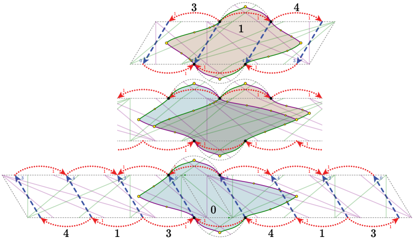
Figure A.1. The first row shows the cross for the equatorial square for tetrahedron 1 in fLLQccecddehqrwjj_20102 . The second row shows the T-shape for the unique (in the universal cover) face shared by tetrahedra 1 and 0. The third row shows the cross for the equatorial square for tetrahedron 0. The corresponding tetrahedron and face rectangles are shaded. The vertices and edges of the dual graph are shown only on the boundary of the rectangles. The cusps are shown with black dots while other regions are indicated with yellow dots. Corners of the rectangles are drawn with larger yellow dots.

As usual, we define $\tau^{X}=X\cap B^{\mathcal{V}}$, and similarly define $\tau_{X}$. These are train-tracks properly embedded in $X$. Let $\tau(X)\subset X$ be the graph dual to the union $\tau^{X}\cup\tau_{X}$. In a small abuse, we place vertices of $\tau(X)$, if dual to a cusp region, at the associated cusp. We call an edge $e^{\prime}$ of $\tau(X)$ upper or lower as its dual edge $e$ lies in $\tau_{X}$ or $\tau^{X}$ respectively. A rectangle in $X$ is an embedded disk in $X$ whose sides in $\tau(X)$ alternate between upper and lower exactly four times.

Lemma A.2.

There is a unique rectangle $R=R(t)$ in $X=X(t)$ so that $\partial R$ meets the vertices of $t$ and is disjoint from all junctions.

Proof.

Fix an edge $e$ of the equatorial square $E=E(t)$. Let $c$ and $d$ be the cusps at the two ends of $e$. Let $Y$ be the component of $X-e$ not containing $E$. Suppose that the junction immediately adjacent to $c$, in $Y$, intersects $\tau^{Y}$. Thus the junction immediately adjacent to $d$, in $Y$, intersects $\tau_{Y}$. Let $F$ be the connected component of $Y-\tau_{Y}$ containing $c$. Similarly, let $G$ be the connected component of $Y-\tau^{Y}$ containing $d$. By Remark 9.16(2) and (5), the regions $F$ and $G$ intersect in a quadragon. We deduce that there is a unique path in the dual graph (to $\tau^{Y}\cup\tau_{Y}$) from $c$ to $d$ that changes from lower to upper, exactly once, and which avoids junctions. See Figure A.1.

Suppose that the junction immediately adjacent to $c$, in $Y$, instead intersects $\tau_{Y}$. Then a similar argument finds a path in the dual graph from $c$ to $d$ that changes from upper to lower, exactly once, and which avoids junctions.

Doing the above for all four edges of $E$ gives the boundary of a rectangle $R=R(t)$. As required, $\partial R$ meets the vertices of $t$ and avoids junctions. The uniqueness of $R$ follows from the slope conditions on the branches of $\tau^{X}$ and $\tau_{X}$ and the requirement that $\partial R$ avoids junctions. ∎

Note that $R(t)$ receives a cellulation from its intersection with $\tau^{X}$ and $\tau_{X}$. We use $R^{(1)}(t)$ to denote the edges of $R(t)$ belonging to $\tau^{X}$. Similarly, $R_{(1)}(t)$ denotes the edges of $R(t)$ belonging to $\tau_{X}$. We now turn to constructing rectangles for the faces of $\mathcal{V}$.

Definition A.3.

Suppose that $f$ is a veering face of $\mathcal{V}$. Let $e_{0}$, $e_{1}$, and $e_{2}$ be its veering edges. Two of these, say $e_{1}$ and $e_{2}$ are the same colour. Let $c_{i}$ be the vertex of $f$ opposite $e_{i}$. Let $W^{\prime}$ be the shearing region (in the shearing decomposition), containing $f$. Let $W$ be the corresponding crimped shearing region. The edges $e_{1}$ and $e_{2}$ are helical in $\partial W$; also there is a longitudinal crimped edge $e^{\prime}_{0}$ in $\partial W$ that cobounds a crimped bigon $B$ with $e_{0}$. Let $n_{0}$ be a small regular neighbourhood of $e_{0}$ taken in $E_{\succ\!\prec}(\mathcal{V})$. Let $s_{0}=n_{0}-B$.

Let $U$ and $V$ be the crimped shearing regions above and below $s_{0}$ respectively. Let $H_{0}$ be the component of $\partial^{-}U\cap\partial^{+}V$ containing $s_{0}$. We take $H$ to be the central cross-section of $W$. We define $T=T(f)=H\cup H_{0}$ to be the T-shape associated to $f$. ∎

The proof of the following is similar to that of Lemma A.2, replacing Remark 9.16 by Corollary 9.18.

Lemma A.4.

There is a unique rectangle $R=R(f)$ in $T=T(f)$ so that $\partial R$ meets the vertices of $f$ and is disjoint from all junctions. ∎

Again, $R(f)$ receives a cellulation from the tracks $\tau^{T}$ and $\tau_{T}$.

Proposition A.5.

Suppose that $f$ is a face of $\mathcal{V}$. Suppose that $t$ and $t^{\prime}$ are the tetrahedra of $\mathcal{V}$ below and above $f$, respectively. Let $T=T(f)$, let $X=X(t)$, and let $X^{\prime}=X(t^{\prime})$. The upwards combinatorial flow from $R(t)\subset X$ to $T$ takes

• distinct cusps to distinct cusps;

• vertices to vertices,

• edges of $R^{(1)}(t)$ to edges of $T^{(1)}$,

• edges of $R_{(1)}(t)$ to edge-paths of $T_{(1)}$, and

• two-cells of $R(t)$ to unions of two-cells of $T$.

There is a similar statement for the downwards combinatorial flow from $R(t^{\prime})\subset X^{\prime}$ to $T$. The images of $R(t)$ and $R(t^{\prime})$ in $T$ have intersection exactly $R(f)$. ∎

One example of Proposition A.5 is shown in Figure A.1.

References

- [1] Ian Agol. Ideal triangulations of pseudo-Anosov mapping tori. In Topology and geometry in dimension three, volume 560 of Contemp. Math., pages 1--17. Amer. Math. Soc., Providence, RI, 2011. arXiv:1008.1606, doi:10.1090/conm/560/11087.
- [2] Ian Agol and Chi Cheuk Tsang. Dynamics of veering triangulations: infinitesimal components of their flow graphs and applications, 2022. arXiv:2201.02706.
- [3] Benjamin A. Burton, Ryan Budney, and William Pettersson and others. Regina: Software for low-dimensional topology, 1999--2023. https://regina-normal.github.io/.
- [4] Danny Calegari. Bounded cochains on 3-manifolds, 2001. https://arxiv.org/abs/math/0111270, doi:10.48550/ARXIV.MATH/0111270.
- [5] Danny Calegari. Foliations and the geometry of 3-manifolds. Oxford Mathematical Monographs. Oxford University Press, Oxford, 2007. http://math.uchicago.edu/~dannyc/books/foliations/foliations.html.
- [6] Joe Christy. Branched surfaces and attractors. I. Dynamic branched surfaces. Trans. Amer. Math. Soc., 336(2):759--784, 1993. doi:10.2307/2154374.
- [7] Baris Coskunuzer. Uniform 1-cochains and genuine laminations. Topology, 45(4):751--784, 2006. https://doi-org.argo.library.okstate.edu/10.1016/j.top.2006.03.002, doi:10.1016/j.top.2006.03.002.
- [8] Marc Culler, Nathan Dunfield, Matthias Goerner, and Jeffrey R. Weeks. SnapPy, a computer program for studying the geometry and topology of three-manifolds. http://snappy.computop.org.
- [9] Sérgio R. Fenley. Foliations with good geometry. J. Amer. Math. Soc., 12(3):619--676, 1999. doi:10.1090/S0894-0347-99-00304-5.
- [10] Steven Frankel, Saul Schleimer, and Henry Segerman. From veering triangulations to link spaces and back again, 2022. arXiv:1911.00006.
- [11] Andreas Giannopoulos, Saul Schleimer, and Henry Segerman. A census of veering structures. https://math.okstate.edu/people/segerman/veering.html.
- [12] Cameron McA. Gordon. The theory of normal surfaces. Based on lecture notes; typeset by Autumn Kent. https://homepages.warwick.ac.uk/~masgar/Articles/Gordon/normal.pdf.
- [13] Craig D. Hodgson, J. Hyam Rubinstein, Henry Segerman, and Stephan Tillmann. Veering triangulations admit strict angle structures. Geom. Topol., 15(4):2073--2089, 2011. arXiv:1011.3695, doi:10.2140/gt.2011.15.2073.
- [14] Marc Lackenby. Taut ideal triangulations of 3-manifolds. Geom. Topol., 4:369--395, 2000. arXiv:math/0003132, doi:10.2140/gt.2000.4.369.
- [15] Michael P. Landry and Chi Cheuk Tsang. Endperiodic maps, splitting sequences, and branched surfaces, 2023. arXiv:2304.14481.
- [16] Lee Mosher. Laminations and flows transverse to finite depth foliations. Preprint, 1996. https://web.archive.org/web/20190829013413/http://andromeda.rutgers.edu/~mosher/.
- [17] R. C. Penner and J. L. Harer. Combinatorics of train tracks, volume 125 of Annals of Mathematics Studies. Princeton University Press, Princeton, NJ, 1992. doi:10.1515/9781400882458.
- [18] Saul Schleimer and Henry Segerman. Veering Dehn surgery. In preparation.
- [19] Saul Schleimer and Henry Segerman. Essential loops in taut ideal triangulations. Algebr. Geom. Topol., 20(1):487--501, 2020. arXiv:1902.03206, doi:10.2140/agt.2020.20.487.
- [20] Saul Schleimer and Henry Segerman. From loom spaces to veering triangulations, 2021. arXiv:2108.10264.
- [21] William P. Thurston. Geometry and topology of three-manifolds. Lecture notes, 1978. http://msri.org/publications/books/gt3m/.
- [22] Chi Cheuk Tsang. Constructing Birkhoff sections for pseudo-Anosov flows with controlled complexity, 2022. arXiv:2206.09586.
- [23] Chi Cheuk Tsang. Veering branched surfaces, surgeries, and geodesic flows, 2022. arXiv:2203.02874.