Model Predictive Control with Reach-avoid Analysis
Abstract
In this paper we investigate the optimal controller synthesis problem, so that the system under the controller can reach a specified target set while satisfying given constraints. Existing model predictive control (MPC) methods learn from a set of discrete states visited by previous (sub-)optimized trajectories and thus result in computationally expensive mixed-integer nonlinear optimization. In this paper a novel MPC method is proposed based on reach-avoid analysis to solve the controller synthesis problem iteratively. The reach-avoid analysis is concerned with computing a reach-avoid set which is a set of initial states such that the system can reach the target set successfully. It not only provides terminal constraints, which ensure feasibility of MPC, but also expands discrete states in existing methods into a continuous set (i.e., reach-avoid sets) and thus leads to nonlinear optimization which is more computationally tractable online due to the absence of integer variables. Finally, we evaluate the proposed method and make comparisons with state-of-the-art ones based on several examples.
1 Introduction
Control synthesis is a fundamental problem which automatically constructs a control strategy that induces a system to exhibit a desired behavior. Due to the ability of handling control and state constraints and yielding high performance control systems Camacho and Alba (2013), control design methods based on MPC have gained great popularity and found wide acceptance in industrial applications, ranging from autonomous driving Verschueren et al. (2014); Kabzan et al. (2019) to large scale interconnected power systems Ernst et al. (2008); Mohamed et al. (2011).
In MPC design methods one issue is to guarantee feasibility of the successive optimization problems Scokaert and Rawlings (1999). Because MPC is ‘greedy’ in its nature, i.e., it only searches for the optimal strategy within a finite horizon, an MPC controller may steer the state to a region starting from where the violation of hard state constraints cannot be avoided. Although this feasibility issue could be solved by using a sufficiently long prediction horizon, we may not be able to afford the computation overhead due to the limited computational resources. Consequently, several solutions towards the feasibility issue are proposed Zheng and Morari (1995); Zeng et al. (2021); Ma et al. (2021). Besides the feasibility issue of satisfying all hard state constraints Zheng and Morari (1995); Zeng et al. (2021); Ma et al. (2021), a system is also desired to achieve certain performance objective in an optimal sense. In existing literature, stability performance of approaching an equilibrium within the MPC framework is extensively studied. One common solution of achieving stability is adding Lyapunov functions as terminal costs and/or corresponding invariant sets as terminal sets Michalska and Mayne (1993); Limon et al. (2005); Limón et al. (2006); Mhaskar et al. (2006); de la Peña and Christofides (2008); Wu et al. (2019); Grandia et al. (2020). This has motivated significant research work on applications of this control design to nonlinear processes Yao and Shekhar (2021). However, in many real applications stability performance is demanding. For example, a spacecraft rendezvous may require the chaser vehicle to be at a certain position relative to the target, moving towards it with a certain velocity. All of these quantities are specified with some tolerance, forming a target region in the state space. When the chaser enters that region a physical connection would be made and the maneuver is complete. However, since the target velocity is non-zero, the region is not invariant and stability cannot be achieved. Regarding this practical issue, the formulation in this paper replaces the notion of stability with reachability: given a target set, the system will achieve the reachability objective of reaching the target set in finite time successfully. To the best of our knowledge, the learning model predictive control (LMPC) proposed in Rosolia and Borrelli (2017), which utilizes the historical data to improve suboptimal controllers iteratively, is the only method within the MPC framework which can solve this problem. However, it leads to mixed-integer nonlinear programming problems which are fundamentally challenging to solve.
In this work, we consider control tasks where the goal is to steer the system from a starting configuration to a target set in finite time, while satisfying state and input constraints. The control task is formalized as a reach-avoid optimization problem. For solving the optimization problem, we propose a novel learning based MPC algorithm which fuses iterative learning control (ILC) Arimoto et al. (1984) and reach-avoid analysis in Zhao et al. (2022). The proposed algorithm utilizes MPC to iteratively improve upon a suboptimal controller. Based on a suboptimal controller obtained in the previous iteration, the reach-avoid analysis is to compute a set of initial states such that the closed-loop system can reach the target set without a violation of the state and input constraints. In our algorithm, the reach-avoid analysis not only provides terminal constraints which ensure feasibility of the MPC, but also expands the viability space of the system and thus facilitates exploring better trajectories with lower costs. Finally, several examples demonstrate the benefits of our algorithm over state-of-the-art ones.
The closest work to the present one is Rosolia and Borrelli (2017). Due to the use of a set of discrete states visited by previous (sub-)optimized trajectories, computationally expensive mixed-integer nonlinear programming problems have to be addressed online in the proposed LMPC, limiting its application in practice. Our method is inspired by Rosolia and Borrelli (2017). However, it incorporates the recently developed reach-avoid analysis technique and expands discrete states into a continuous (reach-avoid) set, which not only facilitates exploring better trajectories but also leads to a novel MPC formulation which involves solving more computationally tractable nonlinear programming problems online. Besides, this work is also close to the ones on model-based safe reinforcement learning, such as Thomas et al. (2021); Luo and Ma (2021); Wen and Topcu (2018). However, these studies prioritize enforcing the safety objective rather than achieving a joint objective of safety and reachability.
2 Preliminaries
In this section we introduce the reach-avoid optimization problem of interest. Throughout this paper, and denote the set of -dimensional real vectors and non-negative integers, respectively. denotes the ring of polynomials in variables given by the argument. represents the set of sum-of-squares polynomials over variable , i.e., .
2.1 Problem Statement
Consider a discrete-time dynamical system
| (1) |
where is the system dynamics, is the state and is the control.
Definition 1.
A control policy is a sequence of control inputs , where . Furthermore, we define as the set of all control policies.
Given a safe set and a target set with , a control policy is safe with respect to a state , if the control policy will drive system (1) starting from to reach the target set in finite time while staying inside the safe set before the first target hitting time. The associated cost of reaching the target set safely is defined below.
Definition 2.
Given a state , and a safe policy , the cost with respect to the state and the policy is defined below:
| (2) |
where , , and is continuous and satisfies
| (3) |
In this paper, we would like to synthesize a safe control policy with respect to a specified initial state such that system (1) will enter the target set with the minimal cost in finite time while staying inside the safe set before the first target hitting time.
Problem 1.
We attempt to solve the following reach-avoid optimization problem:
| (4) |
where is the first time of hitting the target set .
Due to uncertainties on the target hitting time, it is challenging to solve optimization (4) directly. However, the computational complexity can be reduced when searching for a feasible sub-optimal solution. In this paper we will adopt a learning strategy to solving (4), which iteratively improves upon already known suboptimal policies as the LMPC algorithm in Rosolia and Borrelli (2017). Consequently, an initial feasible policy is needed, as formulated in Assumption 1.
Assumption 1.
Remark 1.
The availability of a feasible control policy is not restrictive in practice for a number of applications. For instance, with race cars one can always run a path at very low speed to obtain a control policy.
2.2 Guidance-barrier Functions
In this subsection we introduce guidance-barrier functions. They not only provide terminal constraints in our MPC method escorting system (1) to the target set safely, but also generate a set which curves out a viability space for system (1) to reach the target set safely.
Definition 3.
Given the safe set , target set and a factor , a bounded function is a guidance-barrier function of system (1) with the feedback controller , if it satisfies the following constraints:
| (5) |
where , and is a user-defined positive number.
When is polynomial over , and is semi-algebraic set, i.e., , a set of the form with can be obtained using program (3) in Zhao et al. (2022).
Remark 2.
A reach-avoid set can be computed via solving constraint (5), which is a set of states such that there exists a control policy driving system (1) to enter the target set in finite time while staying inside the safe set before the first target hitting time.
Theorem 1.
Given the safe set , target set and a factor , if is a guidance-barrier function of system (1) with the feedback controller , then is a reach-avoid set.
3 Reach-avoid Model Predictive Control
In this section we elucidate our learning-based algorithm for solving optimization (4) in Problem 1, which is built upon a so-called reach-avoid model predictive control (RAMPC). The proposed RAMPC is constructed based on a guidance-barrier function.
Our RAMPC algorithm is iterative and at each iteration it mainly consists of three steps. The first step is to synthesize a feedback controller by interpolating the suboptimal state-control pair obtained in the previous iteration. Then, a guidance-barrier function satisfying (5) with the synthesized feedback controller is computed. Finally, based on the computed guidance-barrier function a MPC controller, together with its resulting state trajectory, is generated online. The framework of the algorithm is summarized in Alg. 1.
For solving (5) in Alg. 1, when is polynomial over , and , and are semi-algebraic sets, i.e., , the problem of solving constraint (5) can be transformed into a semi-definite programming problem (6),
| (6) |
where , .
Otherwise, sample-based approaches in the context of randomized algorithms Tempo et al. (2013) for robust convex optimization can be employed to solve constraint (5). The basis of these approaches is the Almost Lyapunov condition Liu et al. (2020), which allow the Lyapunov conditions to be violated in restricted subsets of the space while still ensuring stability properties. Although results from these approaches lack rigorous guarantees, nice empirical performances demonstrated the practicality of these approaches in existing literature (e.g., Chang and Gao (2021)). We will revisit it in our future work.
Remark 4.
In the following subsection we will introduce the RAMPC optimization in Alg. 1.
3.1 Reach-avoid Model Predictive Control
This subsection introduces the RAMPC optimization in Alg. 1, which involves solving the MPC optimization problem online :
| (7) |
where the superscript is the iteration index, is the state predicted time steps ahead, computed at time , initialized at with , and similarly for , and is the cost with respect to the state and the control policy .
In (7), the terminal constraint
| (8) |
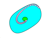
guarantees that the terminal state lies in the reach-avoid set , which carves out a larger continuous viability space (visualized as the cyan region in Fig. 1) for system (1) to be capable of achieving the reach-avoid objective. This is different from the LMCP method in Rosolia and Borrelli (2017), which restricts terminal states within previously explored discrete states (visualized as pink points in Fig. 1) and thus leads to computationally demanding mixed-integer nonlinear optimization. As to the practical computations of the cost , we will give a detailed introduction in Subsection 3.2.
Let
| (9) |
be the optimal solution to (7) at time and the corresponding optimal cost. Then, at time of the iteration , the first element of is applied to the system (1) and thus the state of system (1) turns into
| (10) |
where , which will be the used to update the initial state in (7) for subsequent computations. Once there exist and s.t. , we terminate computations in this iteration: from the state on, we will apply the control actions successively to system (1).
Let be the control policy applied to system (1) by solving optimization (7). The resulting state-control pair , where , is obtained. We can conclude that the performance of is no worse than that of , i.e., . This conclusion can be justified by Theorem 3.
Under Assumption 2, we in Theorem 2 show that the RAMPC (7) is feasible and system (1) with controllers computed by solving (7) satisfies the reach-avoid property, and in Theorem 3 show that the -th iteration cost is non-increasing as increases in RAMPC (7). Their proofs can be found in the appendix.
Assumption 2.
At each iteration the computed reach-avoid set via solving (5) is non-empty. In addition, we assume that it includes the state trajectory 111This assumption can be realized by interpolating the feedback controller s.t. , . This requirement mainly serves for our theoretical analysis since it can guarantee that our algorithm can iteratively improve the policy (Theorem 3). However, in practical this requirement is not indispensable regarding efficient computations..
Theorem 2.
3.2 Estimating Terminal Costs via Scenario Optimization
In practice, the exact terminal cost is challenging, even impossible to obtain. In this subsection, we present a linear programming method based on the scenario optimization Calafiore and Campi (2006) to compute an approximation of the terminal cost in the probably approximately correct (PAC) sense.
Let be the independent samples extracted from according to the uniform distribution , and be the corresponding cost of the roll-out from with the controller . Such cost can be simply computed by summing up the cost along the closed-loop realized trajectory until the target set is reached. Finally, using the set of sample states and correspding costs , we approximate the terminal cost using the scenario optimization Calafiore and Campi (2006).
A linearly parameterized model template , is utilized, which is a linear function in unknown parameters but can be nonlinear over . Then we construct the following linear program over based on the family of given datum :
| (11) |
where is a pre-specified upper bound for , .
Denote the optimal solution to (11) by . The discrepancy between and is formally characterized by two parameters: the error probability and confidence level .
Theorem 4.
Thus, we relax optimization (4) into the following form:
| (12) |
where is the approximate terminal cost at the state , which is obtained via solving (11).
Proposition 1.
With at least confidence,
holds with the probability larger than or equal to , i.e.,
4 Examples
In this section we evaluate our RAMPC algorithm, i.e., Alg. 2, and make comparisons with the LMPC algorithm in Rosolia and Borrelli (2017) on several examples. All the experiments were run on MATLAB 2022b with CPU 12th Gen Intel(R) Core(TM) i9-12900K and RAM 64 GB. Constraint (5) is solved by encoding it into sum-of-squares constraints which is treated by the semi-definite programming solver MOSEK; the nonlinear programming (7) and the mixed-integer nonlinear programming in the LMPC algorithm in Rosolia and Borrelli (2017) are solved using YALMIP Lofberg (2004). In addition, we take as a linear function to interpolate the -th state-control trajectory at each iteration . The configuration parameters in Alg. 2 for all examples are shown in Table 1.
| Example | |||||||
|---|---|---|---|---|---|---|---|
| Ex. 1 | 1.001 | 1 | 4 | 8 | 0.1 | 0.1 | 0.1 |
| Ex. 2 | 1.001 | 1 | 3 | 8 | 0.1 | 0.05 | 0.05 |
| Ex. 3 | 1.001 | 1 | 4 | 6 | 0.002 | 0.1 | 0.1 |
Example 1.
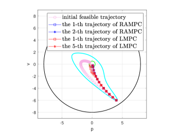
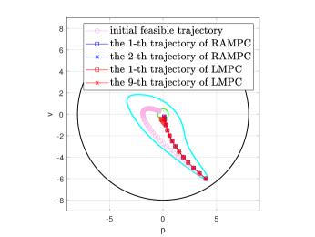
Consider the drone system from Rosolia and Borrelli (2017),
where , and are respectively the position and velocity of the drone at time , is the control input and is the control interval which is equal to .
We assume , initial state , target set and control input set . The set in constraint (5) is obtained by solving a semi-define program as in Zhao et al. (2022). The cost in optimization (4) is . For simplicity of presentation herein, we do not present the initial state-control trajectory which is a long sequence. The initial state-control trajectory is induced by the feedback controller . For scenario optimization (11), we use a template of the polynomial form and sampled points which can be computed via Theorem 4.
We compare our RAMPC algorithm with the LMPC one in Rosolia and Borrelli (2017) with the same prediction horizon and termination conditions (i.e., and ). Since this system is linear, instead of using a set of explored discrete states, the terminal constraint in the LMPC algorithm can be constructed by its convex hull, thus resulting in non-linear programs instead of mixed-integer nonlinear programs as mentioned in Rosolia and Borrelli (2017). The performances of trajectories (shown in Figure 2) generated by both are compared. The iteration costs and computation times at each iteration of RAMPC and LMPC are presented in Table 2. It is observed that the iteration costs in our algorithm drop more quickly than those in the LMPC one. Also, our RAMPC algorithm is more efficient than the LMPC one. RAMPC terminates after iterations with the computation time of , but LMPC converges more slowly and has to take iterations with the computation time of .
| Iteration | Iteration Cost | Time Cost(seconds) | ||
|---|---|---|---|---|
| RAMPC | LMPC | RAMPC | LMPC | |
| 0 | 369.8267 | 369.8267 | ||
| 1 | 215.1007 | 222.2482 | 3.3204 | 3.1741 |
| 2 | 215.1002 | 217.3604 | 3.0100 | 1.5634 |
| 3 | - | 215.3008 | - | 1.1980 |
| 4 | - | 215.1003 | - | 1.1023 |
| 5 | - | 215.1044 | - | 1.1881 |
| total time | 8.2259 | |||
Example 2.
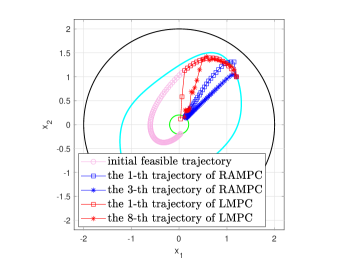
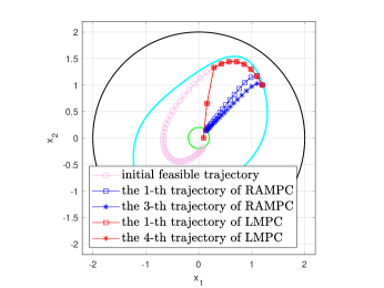
Consider the Euler version with the time step of the controlled reversed-time Van der Pol oscillator in Drazin and Drazin (1992):
with the safe set , initial state , target set and input set .
In (5), the set is computed by solving a semi-define program in Zhao et al. (2022). In addition, the cost , where , is adopted. The initial trajectory is induced by the controller . For scenario optimization (11), we use a template of the polynomial form and samples which can be computed via Theorem 4. LMPC uses the same prediction horizon and termination conditions (i.e., and ).
Some trajectories generated by our RAMPC algorithm and the LMPC algorithm are visualized in Figure 3. Our RAMPC algorithm terminates after the third iteration, but the LMPC one does not terminate after eight iterations. Figure 3 shows that the initial trajectory and the trajectory generated by the first iteration in the LMPC algorithm are too close to be indistinguishable within the first few time steps, which on the other hand further reflects that the controller generated in the first iteration of the LMPC algorithm may not improve the performance induced by the initial control policy. Besides, it is observed that the eighth trajectory from the LMPC algorithm looks not stable and has strong oscillations, which are not expected in practice. In contrast, the trajectory generated by our algorithm is smoother.
Table 3 summarizes the iteration costs and the computation times at each iteration of our RAMPC algorithm and the LMPC one. The iteration cost induced by the initial trajectory is , after three iterations our RAMPC algorithm reduces the cost to with the computation time of . In contrast, the LMPC algorithm needs more than 8 iterations with the computation time of almost more than hours to achieve the same cost. This striking contrast definitely demonstrates that our RAMPC algorithm can solve optimization (4) more efficiently for some cases.
| Iteration | Iteration Cost | Time Cost(seconds) | ||
|---|---|---|---|---|
| RAMPC | LMPC | RAMPC | LMPC | |
| 0 | 64.3087 | 64.3087 | ||
| 1 | 30.9693 | 40.0714 | 10.6583 | 45.0 |
| 2 | 29.2919 | 39.3270 | 10.2248 | 59.4 |
| 3 | 29.2824 | 38.5239 | 10.4010 | 558.5 |
| 4 | - | 37.6402 | - | 1298 |
| 5 | - | 36.7088 | - | 1653.3 |
| 6 | - | 35.7561 | - | 2033.6 |
| 7 | - | 35.2567 | - | 2115.2 |
| 8 | - | 34.9022 | - | 1706.1 |
| total time | 9469.1 | |||
Example 3.
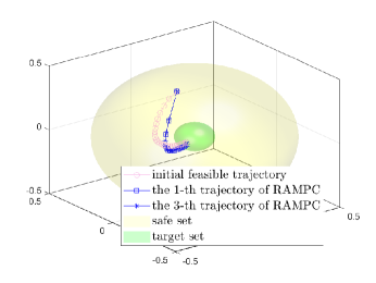
Consider the Euler version with the time step of the controlled 3D Van der Pol oscillator from Korda et al. (2014):
with the safe set , initial state , target set and input set .
The set is utilized in (5) by solving a semi-define program, as described in Zhao et al. (2022). We use the cost function in this example, where . The initial trajectory is generated by the controller . The template of the polynomial form and sample number computed through Theorem 4 are adopted for scenario optimization (11). The prediction horizon and termination condition are same for LMPC.
In this example, LMPC is unable to achieve the desired task of reducing the iteration cost and generating a suitable controller. In contrast, our RAMPC algorithm demonstrates good performance and can generate an effective controller. Table 4 summarizes the iteration costs and computation times at each iteration of our RAMPC algorithm. The initial trajectory and ones generated in the first and last iterations of our RAMPC algorithm are visualized in Figure 4.
| Iteration | Iteration Cost | Time Cost(seconds) |
|---|---|---|
| 0 | 1.3489 | |
| 1 | 0.8344 | 7.8186 |
| 2 | 0.8295 | 7.8022 |
| 3 | 0.8291 | 7.7416 |
| total time | 23.3623 |
Discussions on configuration parameters.
Here we give a brief discussion on the configuration parameters: based on the experiments (some are presented in the appendix). The less conservative the computed reach-avoid set in each iteration is, the smaller the iteration cost is. Therefore, is recommended to be as close to one as possible, but it cannot be one. For details, please refer to Zhao et al. (2022); the upper bound can be any positive number since if satisfies constraint (5) with , then also satisfies constraint (5) with ; and , especially , affect the number of iterations and thus the quality of controllers. Generally, a larger and/or smaller will improve the control performance, but the computational burden increases; the approximation error for terminal costs is formally characterized in the PAC sense using and . These two parameters and the size of parameters determine the minimal number of samples for approximating terminal costs according to Theorem 4. Smaller and will lead to more accurate approximations of terminal costs in the PAC sense. However, regarding the overfitting issue and the computational burden of solving (11), too small and are not desired in practice; the prediction horizon controls how far into the future the MPC predicts the system response. Like other MPC schemes, a longer horizon generally increases the control performance, but requires an increasingly powerful computing platform (due to solving (7) online), excluding certain control applications. In practice, an appropriate choice strongly depends on computational resources and real-time requirements. In addition, it is worth remarking here that the costs obtained by RAMPC are not sensitive to for some cases. For details, please refer to experimental results in the appendix.
5 Conclusion
In this paper we proposed a novel RAMPC algorithm for solving a reach-avoid optimization problem. The RAMPC algorithm is built upon MPC and reach-avoid analysis. Rather than solving computationally intractable mixed-integer nonlinear optimization online, it addresses computationally more tractable nonlinear optimization. Moreover, due to the incorporation of reach-avoid analysis, which expands the viability space, the RAMPC algorithm can provide better controllers with a smaller number of iterations. Several numerical examples demonstrated the advantages of our RAMPC algorithm.
Acknowledgments
This research was supported by the NSFC under grant No. 61836005, CAS Project for Young Scientists in Basic Research under grant No. YSBR-040, NSFC under grant No. 52272329, and CAS Pioneer Hundred Talents Program.
References
- Arimoto et al. [1984] Suguru Arimoto, Sadao Kawamura, and Fumio Miyazaki. Bettering operation of robots by learning. Journal of Robotic systems, 1(2):123–140, 1984.
- Calafiore and Campi [2006] Giuseppe Carlo Calafiore and Marco C Campi. The scenario approach to robust control design. IEEE Transactions on Automatic Control, 51(5):742–753, 2006.
- Camacho and Alba [2013] Eduardo F Camacho and Carlos Bordons Alba. Model predictive control. Springer science & business media, 2013.
- Chang and Gao [2021] Ya-Chien Chang and Sicun Gao. Stabilizing neural control using self-learned almost lyapunov critics. In Proceedings of the 2021 IEEE International Conference on Robotics and Automation, pages 1803–1809. IEEE, 2021.
- de la Peña and Christofides [2008] David Muñoz de la Peña and Panagiotis D Christofides. Lyapunov-based model predictive control of nonlinear systems subject to data losses. IEEE Transactions on Automatic Control, 53(9):2076–2089, 2008.
- Drazin and Drazin [1992] Philip G Drazin and Philip Drazin Drazin. Nonlinear systems. Number 10. Cambridge University Press, 1992.
- Ernst et al. [2008] Damien Ernst, Mevludin Glavic, Florin Capitanescu, and Louis Wehenkel. Reinforcement learning versus model predictive control: a comparison on a power system problem. IEEE Transactions on Systems, Man, and Cybernetics, Part B (Cybernetics), 39(2):517–529, 2008.
- Grandia et al. [2020] Ruben Grandia, Andrew J Taylor, Andrew Singletary, Marco Hutter, and Aaron D Ames. Nonlinear model predictive control of robotic systems with control lyapunov functions. arXiv preprint arXiv:2006.01229, 2020.
- Kabzan et al. [2019] Juraj Kabzan, Lukas Hewing, Alexander Liniger, and Melanie N Zeilinger. Learning-based model predictive control for autonomous racing. IEEE Robotics and Automation Letters, 4(4):3363–3370, 2019.
- Korda et al. [2014] Milan Korda, Didier Henrion, and Colin N Jones. Controller design and region of attraction estimation for nonlinear dynamical systems. IFAC Proceedings Volumes, 47(3):2310–2316, 2014.
- Limon et al. [2005] Daniel Limon, Teodoro Alamo, and Eduardo F Camacho. Enlarging the domain of attraction of mpc controllers. Automatica, 41(4):629–635, 2005.
- Limón et al. [2006] Daniel Limón, Teodoro Alamo, Francisco Salas, and Eduardo F Camacho. On the stability of constrained mpc without terminal constraint. IEEE Transactions on Automatic Control, 51(5):832–836, 2006.
- Liu et al. [2020] Shenyu Liu, Daniel Liberzon, and Vadim Zharnitsky. Almost lyapunov functions for nonlinear systems. Automatica, 113:108758, 2020.
- Lofberg [2004] Johan Lofberg. Yalmip: A toolbox for modeling and optimization in matlab. In Proceedings of the 2004 IEEE International Conference on Robotics and Automation (IEEE Cat. No.04CH37508), pages 284–289. IEEE, 2004.
- Luo and Ma [2021] Yuping Luo and Tengyu Ma. Learning barrier certificates: Towards safe reinforcement learning with zero training-time violations. Advances in Neural Information Processing Systems, 34:25621–25632, 2021.
- Ma et al. [2021] Haitong Ma, Xiangteng Zhang, Shengbo Eben Li, Ziyu Lin, Yao Lyu, and Sifa Zheng. Feasibility enhancement of constrained receding horizon control using generalized control barrier function. In Proceedings of the 4th IEEE International Conference on Industrial Cyber-Physical Systems, pages 551–557. IEEE, 2021.
- Mhaskar et al. [2006] Prashant Mhaskar, Nael H El-Farra, and Panagiotis D Christofides. Stabilization of nonlinear systems with state and control constraints using lyapunov-based predictive control. Systems & Control Letters, 55(8):650–659, 2006.
- Michalska and Mayne [1993] Hannah Michalska and David Q Mayne. Robust receding horizon control of constrained nonlinear systems. IEEE Transactions on Automatic Control, 38(11):1623–1633, 1993.
- Mohamed et al. [2011] TH Mohamed, H Bevrani, AA Hassan, and T Hiyama. Decentralized model predictive based load frequency control in an interconnected power system. Energy Convers. Manag., 52(2):1208–1214, 2011.
- Rosolia and Borrelli [2017] Ugo Rosolia and Francesco Borrelli. Learning model predictive control for iterative tasks. a data-driven control framework. IEEE Transactions on Automatic Control, 63(7):1883–1896, 2017.
- Scokaert and Rawlings [1999] Pierre OM Scokaert and James B Rawlings. Feasibility issues in linear model predictive control. AIChE Journal, 45(8):1649–1659, 1999.
- Tempo et al. [2013] Roberto Tempo, Giuseppe Calafiore, and Fabrizio Dabbene. Randomized algorithms for analysis and control of uncertain systems: with applications. Springer, 2013.
- Thomas et al. [2021] Garrett Thomas, Yuping Luo, and Tengyu Ma. Safe reinforcement learning by imagining the near future. Advances in Neural Information Processing Systems, 34:13859–13869, 2021.
- Verschueren et al. [2014] Robin Verschueren, Stijn De Bruyne, Mario Zanon, Janick V Frasch, and Moritz Diehl. Towards time-optimal race car driving using nonlinear mpc in real-time. In Proceedings of the 53rd IEEE Conference on Decision and Control, pages 2505–2510. IEEE, 2014.
- Wen and Topcu [2018] Min Wen and Ufuk Topcu. Constrained cross-entropy method for safe reinforcement learning. Advances in Neural Information Processing Systems, 31, 2018.
- Wu et al. [2019] Zhe Wu, Fahad Albalawi, Zhihao Zhang, Junfeng Zhang, Helen Durand, and Panagiotis D Christofides. Control lyapunov-barrier function-based model predictive control of nonlinear systems. Automatica, 109:108508, 2019.
- Yao and Shekhar [2021] Ye Yao and Divyanshu Kumar Shekhar. State of the art review on model predictive control (mpc) in heating ventilation and air-conditioning (hvac) field. Build. Environ., 200:107952, 2021.
- Zeng et al. [2021] Jun Zeng, Bike Zhang, and Koushil Sreenath. Safety-critical model predictive control with discrete-time control barrier function. In Proceedings of the 2021 American Control Conference, pages 3882–3889. IEEE, 2021.
- Zhao et al. [2022] Changyuan Zhao, Shuyuan Zhang, Lei Wang, and Bai Xue. Inner-approximating robust reach-avoid sets for discrete-time polynomial dynamical systems. IEEE Transactions on Automatic Control, 2022.
- Zheng and Morari [1995] Alex Zheng and Manfred Morari. Stability of model predictive control with mixed constraints. IEEE Transactions on Automatic Control, 40(10):1818–1823, 1995.
Appendix I
The proof of Theorem 2:
Proof.
We firstly prove the RAMPC (7) satisfies recursive feasibility for at every iteration .
1) Assume that the -th iteration the trajectory generated by RAMPC (7) is feasible (when , the initial trajectory is feasible), then we will show that at time of the -th iteration the RAMPC (7) is feasible.
At time of the -th iteration the first steps trajectory
| (13) |
with the related input sequence,
| (14) |
satisfies the constraints in (7), thus (13) and (14) is a feasible solution of RAMPC (7) at of the -th iteration.
2). Assume that at time of the -th iteration the RAMPC (7) is feasible, then we will show that at time of the -th iteration RAMPC (7) is feasible.
Let and in (9) be the optimal trajectory and input sequence at time .
We define . With the fact that is a reach-avoid set with the controller , and the first constraint in (5), we have which satisfies the terminate constraint (8).
At time of the -th iteration the input sequence
| (15) |
with the related feasible state trajectory,
| (16) |
satisfies the constraints in (7), Thus (15) and (16) is a feasible solution for RAMPC (7) at time .
With the principle of induction, the RAMPC (7) is feasible for and .
Next we will prove that the resulting trajectory (as shown in (10)) at iteration satisfies the reach-avoid property. According to the terminate constraint (8), we have that
i.e. , If the trajectory never reach the target set , then , which contracts the fact that is bounded over the compact set . Consequently, there exists such that and thus . Also, from the constraint , we have that (see Remark 2) and thus . ∎
The proof of Theorem 3:
Appendix II
Example 4.
Consider the system in Example 1, but with the different configurations in Table 5. Table 6 summarizes the costs obtained at each iteration of our RAMPC algorithm and the LMPC one, and Table 7 shows the computation times of each iteration for these two algorithms. Some trajectories generated by our RAMPC algorithm and the LMPC algorithm are visualized in Figure 5.
| Iteration | Iteration Cost | |
|---|---|---|
| RAMPC | LMPC | |
| 0 | 369.8267 | 369.8267 |
| 1 | 215.1011 | 217.1582 |
| 2 | 215.1025 | 216.0086 |
| 3 | - | 215.5209 |
| 4 | - | 215.2383 |
| 5 | - | 215.1722 |
| 6 | - | 215.1324 |
| 7 | - | 215.1106 |
| 8 | - | 215.1003 |
| 9 | - | 215.1007 |
| Iteration | Time Cost(seconds) | |
|---|---|---|
| RAMPC | LMPC | |
| 3.3884 | 2.6410 | |
| 2.7991 | 1.4724 | |
| - | 1.0895 | |
| - | 1.0568 | |
| - | 1.0892 | |
| - | 1.0536 | |
| - | 1.0428 | |
| - | 1.1520 | |
| - | 1.0190 | |
| total | 11.6164 | |
Example 5.
Consider the system in Example 2 with and the different configurations in Table 8. Table 9 summarizes the costs obtained at each iteration of our RAMPC algorithm and the LMPC one, and Table 10 shows the computation times of each iteration for these two algorithms. Some trajectories generated by our RAMPC algorithm and the LMPC algorithm are visualized in Figure 6.
| Iteration | Iteration Cost | |
|---|---|---|
| RAMPC | LMPC | |
| 0 | 36.0724 | 36.0724 |
| 1 | 15.4891 | 20.4661 |
| 2 | 15.1858 | 21.3654 |
| 3 | 15.1860 | 20.4661 |
| 4 | - | 20.4661 |
| Iteration | Time Cost(seconds) | |
|---|---|---|
| RAMPC | LMPC | |
| 5.2348 | 208.7463 | |
| 5.0935 | 142.7198 | |
| 5.0953 | 9.9840 | |
| - | 6.4926 | |
| total | 367.9428 | |
Example 6.
Consider the system in Example 2 with :
- a
- b
| Iteration | Iteration Cost | |||||
|---|---|---|---|---|---|---|
| 2 | 4 | 6 | 8 | 10 | 12 | |
| 0 | 36.0724 | 36.0724 | 36.0724 | 36.0724 | 36.0724 | 36.0724 |
| 1 | 15.4891 | 16.4719 | 15.3693 | 15.3882 | 15.2546 | 15.1886 |
| 2 | 15.1858 | 15.2198 | 15.1777 | 15.1640 | 15.1755 | 15.1703 |
| 3 | 15.1860 | 15.1696 | 15.1673 | 15.1690 | 15.1714 | 15.1719 |
| Iteration | Time Cost | |||||
|---|---|---|---|---|---|---|
| 2 | 4 | 6 | 8 | 10 | 12 | |
| 1 | 5.2348 | 5.2193 | 5.9456 | 3.9578 | 4.1903 | 3.5610 |
| 2 | 5.0935 | 5.2343 | 5.8533 | 5.9139 | 6.0883 | 6.2036 |
| 3 | 5.0953 | 5.6513 | 5.6288 | 6.3013 | 6.9170 | 6.4566 |
| total | 15.4236 | 16.1050 | 17.4276 | 16.1730 | 17.1956 | 16.2212 |
| Iteration | Iteration Cost | |||||
|---|---|---|---|---|---|---|
| 2 | 4 | 6 | 8 | 10 | 12 | |
| 0 | 36.0724 | 36.0724 | 36.0724 | 36.0724 | 36.0724 | 36.0724 |
| 1 | 17.0569 | 16.5073 | 15.8408 | 15.4489 | 15.2860 | 15.2233 |
| 2 | 15.1790 | 15.2286 | 15.1805 | 15.1731 | 15.1641 | 15.1661 |
| 3 | 15.1990 | 15.1678 | 15.1661 | 15.1777 | 15.1922 | 15.1703 |
| Iteration | Time Cost | |||||
|---|---|---|---|---|---|---|
| 2 | 4 | 6 | 8 | 10 | 12 | |
| 1 | 5.4749 | 4.7185 | 5.9308 | 6.3891 | 9.3374 | 7.7943 |
| 2 | 5.1461 | 5.5312 | 6.5768 | 6.3372 | 6.4644 | 8.1602 |
| 3 | 5.4065 | 5.3546 | 5.6288 | 7.1605 | 6.8632 | 9.3544 |
| total | 16.0275 | 15.6043 | 17.4276 | 19.8869 | 22.6650 | 25.3089 |