Recyclable Tuning for Continual Pre-training

Abstract

Continual pre-training is the paradigm where pre-trained language models (PLMs) continually acquire fresh knowledge from growing data and gradually get upgraded. Before an upgraded PLM is released, we may have tuned the original PLM for various tasks and stored the adapted weights. However, when tuning the upgraded PLM, these outdated adapted weights will typically be ignored and discarded, causing a potential waste of resources. We bring this issue to the forefront and contend that proper algorithms for recycling outdated adapted weights should be developed. To this end, we formulate the task of recyclable tuning for continual pre-training. In pilot studies, we find that after continual pre-training, the upgraded PLM remains compatible with the outdated adapted weights to some extent. Motivated by this finding, we analyze the connection between continually pre-trained PLMs from two novel aspects, i.e., mode connectivity, and functional similarity. Based on the corresponding findings, we propose both an initialization-based method and a distillation-based method for our task. We demonstrate their feasibility in improving the convergence and performance for tuning the upgraded PLM. We also show that both methods can be combined to achieve better performance. The source codes are publicly available at https://github.com/thunlp/RecyclableTuning.

1 Introduction

The emergence of pre-trained language models (PLMs) has revolutionized the entire field of natural language processing (NLP) (Bommasani et al., 2021). Through downstream adaptation, PLMs effectively stimulate the knowledge acquired during pre-training and achieve remarkable success in various downstream tasks (Devlin et al., 2019; Liu et al., 2019; Raffel et al., 2020). Such adaptation can be achieved by either full-parameter fine-tuning or parameter-efficient tuning (Houlsby et al., 2019), and the latter enables learning lightweight adapted modules for downstream tasks. Currently, a de facto paradigm for handling NLP tasks has been formed, dividing practitioners into two groups: (1) upstream suppliers, who pre-train PLMs on task-agnostic data and release them on public platforms, e.g., HuggingFace (Wolf et al., 2020), and (2) downstream consumers, who download the PLM and conduct personalized adaptation using task-specific data. The corresponding adapted weights might then be shared with third parties via platforms such as AdapterHub (Pfeiffer et al., 2020).

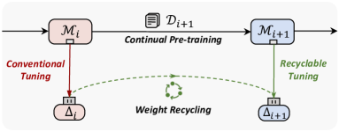
Figure 1: Task formulation. The original PLM $\mathcal{M}_{i}$ is upgraded to $\mathcal{M}_{i+1}$ through continual pre-training on emerging data $\mathcal{D}_{i+1}$. Our goal is to recycle the existing adapted weights $\Delta_{i}$ of $\mathcal{M}_{i}$ for tuning $\mathcal{M}_{i+1}$.

In real-world scenarios, PLMs may constantly get upgraded and released by the supplier. Correspondingly, the customer-side compatible update of adapted weights becomes necessary. Continual pre-training (Qin et al., 2022c) is a typical scenario where PLMs continually acquire fresh knowledge from growing data and gradually get upgraded. Before an upgraded PLM is released, consumers may have tuned the original PLM for various tasks and stored the adapted weights. However, when tuning the upgraded PLM, these outdated adapted weights will typically be ignored and discarded. This can lead to a loss of knowledge about downstream tasks encapsulated in the outdated weights, as well as a potential waste of computational resources. In this paper, we bring this issue to the forefront and argue that proper algorithms for recycling outdated adapted weights should be developed. To this end, we formulate the task of recyclable tuning for continual pre-training, which is illustrated in Figure 1.

Due to the parameter change during continual pre-training, one potential concern for recycling outdated adapted weights is their mismatch with the upgraded PLM. However, our pilot studies reveal that directly applying the outdated weights to the upgraded PLM yields substantial performance improvements as compared to zero-shot inference of the PLM. This shows that the upgraded PLM remains compatible with the outdated weights to some extent, indicating a close connection between continually pre-trained PLMs. Intuitively, such a connection provides a strong basis for our assertion that outdated weights are recyclable and useful.

To uncover hints for solving our task, we further investigate such a connection from two aspects: (1) linear mode connectivity (Qin et al., 2022b). We demonstrate that after adapting both the upgraded PLM and the original PLM to the same task, linearly interpolating the parameters of both adapted models could produce a series of checkpoints with high task performance (low loss). Such a property indicates a close parametric connection of both PLMs in the loss landscape; (2) functional similarity. After adapting both PLMs to the same task, we observe that their corresponding attention heads exhibit similar patterns given the same input. Such representational proximity implies that both PLMs own similar functionalities during text processing.

Both analyses above demonstrate the close connections between continually pre-trained PLMs. Based on the corresponding findings, we propose two methods for recyclable tuning:

(1) Initialization-based method, which leverages the adapted weights of the original PLM as the initialization for the upgraded PLM. This method is motivated by their close parametric connection in the loss landscape. We demonstrate that for a target task, initializing the tunable parameters with the outdated weights from a similar source task could accelerate the convergence and improve the training efficiency, compared to using random initialization. In addition, after sufficient training, this method generally improves the final performance. We also observe that the benefits of this method in terms of convergence and performance are greater when the source and target tasks are more similar.

(2) Distillation-based method, which distills the knowledge stored in outdated weights for tuning the upgraded PLM. We demonstrate that knowledge distillation can effectively facilitate knowledge transfer between continually pre-trained PLMs. Using only a small number of labeled examples, the upgraded PLM can outperform the original PLM when trained with far more examples. We also show that both initialization-based and distillation-based methods can be combined to further improve the performance. This means knowledge transfer through parameter space and model outputs are complementary to each other.

In a nutshell, these results highlight the practical benefits of recyclable tuning and point to an important future direction in sustainable NLP.

2 Related Work

Continual Pre-training.

Conventionally, PLMs are trained on static data, ignoring that streaming data from various sources could continually grow. Continual pre-training requires PLMs to accumulate new knowledge in a continual manner (Gururangan et al., 2020), meanwhile alleviating the catastrophic forgetting problem. Prior works in this field focus on building benchmarks and analyses (Jang et al., 2021, 2022). Later works explored the applicability of traditional continual learning algorithms under this setting (Jin et al., 2022; Wu et al., 2021). Recent efforts were also spent on continual pre-training in a computationally efficient way (Qin et al., 2022c).

Previous works focus on improving the capabilities of PLMs during pre-training from the standpoint of upstream suppliers. Instead, we shift the focus to downstream adaptation from the perspective of customers. We highlight a previously overlooked issue of the incompatibility between upgraded PLMs and the existing adapted weights. For the first time, we examine the connections between continually pre-trained models and demonstrate the potential benefits of recycling outdated weights.

Knowledge Transfer for PLMs.

Transfer learning for PLMs has gained increasing attention recently. Some works study task-level transferability for an individual PLM and find that fine-tuning on certain source tasks conduces to the performance on similar target tasks (Vu et al., 2020; Poth et al., 2021; Aghajanyan et al., 2021). Differently, we also study cross-task knowledge transfer for two different PLMs under the continual pre-training scenario (§ 5.1). Besides, researchers also investigate cross-model knowledge transfer. They try to recycle lightweight adapted weights of the same task between two independently pre-trained PLMs, e.g., PLMs with distinct data (Su et al., 2022). As we would show later, unlike independently trained PLMs, continually pre-trained PLMs are guaranteed close connections. This distinction determines our setting is unique to previous works and may require different solutions.

3 Problem Formulation

Continual Pre-training.

Following Qin et al. (2022c), we simulate the scenario where new data from $4$ domains is gathered sequentially, i.e., biomedical papers (Bio, $\mathcal{D}_{1}$) (Lo et al., 2020), amazon reviews (Rev, $\mathcal{D}_{2}$) (He and McAuley, 2016), computer science papers (CS, $\mathcal{D}_{3}$) (Lo et al., 2020), and news articles (Ns, $\mathcal{D}_{4}$) (Zellers et al., 2019). Starting from the official $\text{RoBERTa}_{\texttt{BASE}}$ (Liu et al., 2019) (denoted as $\mathcal{M}_{0}$), we continually pre-train $\mathcal{M}_{0}$ on $4$ domains. For each domain, we set the pre-training steps to $12.5$k and the batch size to $2048$. Denote $\mathcal{M}_{i}$ as the PLM that finishes training on $\mathcal{D}_{i}$, and $\mathcal{M}_{i}(t)$ as the PLM that starts from $\mathcal{M}_{i-1}$ and is trained on $\mathcal{D}_{i}$ for $t$ steps. We assume the suppliers only release the PLM that finishes training on each domain, i.e., $\{\mathcal{M}_{\text{1}},\cdots,\mathcal{M}_{\text{4}}\}$ are developed and released. The pre-training details are described in § D.1.

Downstream Adaptation.

At the same time, we have a set of downstream tasks to handle. To adapt $\mathcal{M}_{i}$ ($0\!\leq\!i\leq 4$) towards a task $\mathcal{T}_{j}$, we conduct supervised training using the loss function $\mathcal{L}_{\mathcal{T}_{j}}$. Denote the pre-trained weights of $\mathcal{M}_{i}$ as $\theta_{i}^{0}$, we obtain its adapted weights $\Delta_{i}^{\mathcal{T}_{j}}$ for $\mathcal{T}_{j}$ after training. By assembling both $\theta_{i}^{0}$ and $\Delta_{i}^{\mathcal{T}_{j}}$, the resultant model $\theta_{i}^{\mathcal{T}_{j}}\!=\!\theta_{i}^{0}\!\oplus\!\Delta_{i}^{\mathcal{T}_{j}}$ can be deployed to handle $\mathcal{T}_{j}$. Throughout this paper, we consider two tuning methods: full-parameter fine-tuning and a representative parameter-efficient tuning method, adapter tuning (Houlsby et al., 2019) (see § A.1 for more backgrounds). For the former, we have $|\Delta_{i}^{\mathcal{T}_{j}}|\!=\!|\theta_{i}^{0}|$; while for the latter, $|\Delta_{i}^{\mathcal{T}_{j}}|\!\ll\!|\theta_{i}^{0}|$, where $|\cdot|$ denotes the number of parameters.

Recyclable Tuning.

Before the release of an upgraded PLM $\mathcal{M}_{i^{\prime}}$ ($i\!<\!i^{\prime}$), we have obtained adapted weights $\Delta_{i}^{\mathcal{T}_{j}}$ of an old PLM $\mathcal{M}_{i}$ for task $\mathcal{T}_{j}$. Recyclable tuning aims at transferring the knowledge of $\Delta_{i}^{\mathcal{T}_{j}}$ to assist tuning $\mathcal{M}_{i^{\prime}}$ (i.e., learning new weights $\Delta_{i^{\prime}}^{\mathcal{T}_{j}}$). We denote the above process as $\Delta_{i}^{\mathcal{T}_{j}}\!\rightarrow\!\Delta_{i^{\prime}}^{\mathcal{T}_{j}}$. Intuitively, $\Delta_{i}^{\mathcal{T}_{j}}$ encapsulates abundant knowledge about the task $\mathcal{T}_{j}$, which should benefit learning $\Delta_{i^{\prime}}^{\mathcal{T}_{j}}$ if exploited properly. Such benefits may include improving training efficiency or performance. To gain insights of solving the task, we first conduct a series of empirical analyses in § 4 to understand the connections among $\mathcal{M}_{i}$, $\mathcal{M}_{i^{\prime}}$, $\Delta_{i}^{\mathcal{T}_{j}}$, and $\Delta_{i^{\prime}}^{\mathcal{T}_{j}}$.

4 Empirical Analysis

We first investigate the compatibility of outdated weights and the upgraded PLM (§ 4.1), then we explore the (1) parametric connections and (2) representational connections of continually pre-trained PLMs from two aspects: (1) linear mode connectivity (§ 4.2) and (2) functional similarity (§ 4.3). The implementation details are left in § D.2.

4.1 Model Compatibility Analysis

We explore to what extent the outdated weights are compatible with the upgraded PLM and how this compatibility changes during continual pre-training. Specifically, we directly apply outdated weights to the upgraded PLM and record the performance variation during continual pre-training.

Settings.

We first investigate the process when upgrading $\mathcal{M}_{0}$ to $\mathcal{M}_{1}$ on the Bio domain ($\mathcal{D}_{1}$). For downstream evaluation, we choose two classification tasks: ChemProt (Kringelum et al., 2016), which is a relevant downstream task to the Bio domain, and MNLI (Williams et al., 2018). Denote the model continually pre-trained on $\mathcal{D}_{1}$ for $t$ steps as $\mathcal{M}_{1}(t)$, its pre-trained weights as $\theta_{1}^{0}(t)$, and the adapted weights of $\mathcal{M}_{0}$ for the downstream task as $\Delta_{0}^{\mathcal{T}}$. We directly apply $\Delta_{0}^{\mathcal{T}}$ to the upgraded PLM $\mathcal{M}_{1}(t)$, i.e., $\theta_{1}^{0}(t)\oplus\Delta_{0}^{\mathcal{T}}$, and evaluate the performance on the test set of the downstream task. In experiments, $t$ is selected from $1.25$k to $12.5$k with an interval of $1.25$k. We also report $\mathcal{M}_{1}(t)$’s zero-shot inference performance by testing $\theta_{1}^{0}(t)$.

Results.

From the results in Figure 2 (a, b), we observe that for both adapter and fine-tuning: (1) with $t$ increasing, the performance of $\theta_{1}^{0}(t)\!\oplus\!\Delta_{0}^{\mathcal{T}}$ drops quickly at first. This means that $\Delta_{0}^{\mathcal{T}}$ becomes outdated shortly after the backbone model $\mathcal{M}_{1}(t)$ changes. (2) After sufficient pre-training steps, the performance converges to a plateau which is still much higher than the zero-shot inference performance of $\mathcal{M}_{1}(t)$. This implies that continually pre-trained PLMs are intrinsically connected with their “ancestors”, otherwise the ancestor’s adapted weights $\Delta_{0}^{\mathcal{T}}$ would not improve the performance of its offspring $\mathcal{M}_{1}(t)$.

Extension to Multiple Domains.

Next, we extend the above experiments to $4$ sequentially released PLMs as mentioned in § 3 by directly applying $\Delta_{0}^{\mathcal{T}}$ to $\{\mathcal{M}_{1},\cdots,\mathcal{M}_{4}\}$. We derive from Figure 2 (c, d) that: (1) applying outdated weights consistently performs better than zero-shot inference even if the backbone PLM is trained over multiple domains; (2) the performance of $\mathcal{M}_{4}$ is the best among $\{\mathcal{M}_{1},\cdots,\mathcal{M}_{4}\}$ though $\mathcal{M}_{4}$ is trained for the longest time. This may be because the Ns domain ($\mathcal{D}_{4}$) is the most similar one to $\mathcal{M}_{0}$’s pre-training data (Gururangan et al., 2020), and continual pre-training on a similar domain of the original PLM mitigates the incompatibility.

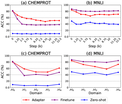
Figure 2: (a, b): performance variation w.r.t. pre-training steps ($t$) when applying the outdated weights ($\Delta_{0}^{\mathcal{T}}$) to $\mathcal{M}_{1}(t)$. (c, d): performance variation when applying the outdated weights ($\Delta_{0}^{\mathcal{T}}$) to $\{\mathcal{M}_{1},\cdots,\mathcal{M}_{4}\}$.

4.2 Linear Mode Connectivity Analysis

Backgrounds.

Linear mode connectivity measures whether two sets of model weights can be connected via a linear parametric path, along which the performance (loss) of the downstream task remains high (low) (Frankle et al., 2020). In other words, it tests whether linear interpolations of two model weights perform comparably to both endpoints. If this property holds, then both model weights probably lie in the same loss basin, which indicates a close connection between them in the parameter space (Qin et al., 2022b). For more detailed backgrounds, please refer to § A.2.

Settings.

Following most of the settings in § 4.1, we adapt both $\mathcal{M}_{0}$ and $\mathcal{M}_{1}(t)$ towards the task ChemProt and obtain the weights $\theta_{0}^{\mathcal{T}}$ and $\theta_{1}^{\mathcal{T}}(t)$, where $\theta_{0}^{\mathcal{T}}=\theta_{0}^{0}\oplus\Delta_{0}^{\mathcal{T}}$ and $\theta_{1}^{\mathcal{T}}(t)=\theta_{1}^{0}(t)\oplus\Delta_{1}^{\mathcal{T}}(t)$. Then we linearly interpolate both $\theta_{0}^{\mathcal{T}}$ and $\theta_{1}^{\mathcal{T}}(t)$ as:

$$\theta(\mu)=(1-\mu)\theta_{0}^{\mathcal{T}}+\mu\theta_{1}^{\mathcal{T}}(t),$$ (1)

where $\mu\in(0,1)$. In experiments, we evaluate the performance of $25$ evenly distributed interpolations and two endpoints (i.e., $\mu=0$ and $\mu=1$). If there does not exist a significant performance drop along the linear path, we deem both endpoints linearly mode connected. We choose $\mathcal{M}_{1}(t)$ that is continually pre-trained for $\{2.5,5.0,7.5,10.0,12.5\}$k steps and evaluate mode connectivity for each $\mathcal{M}_{1}(t)$ and $\mathcal{M}_{0}$. In addition, we pre-train a new $\text{RoBERTa}_{\texttt{BASE}}$ (dubbed as $\mathcal{M}_{\text{IND}}$) from scratch (details in § D.1) and test its connectivity with $\mathcal{M}_{0}$, i.e., $\theta(\mu)\!=\!(1\!-\!\mu)\theta_{0}^{\mathcal{T}}\!+\!\mu\theta_{\text{IND}}^{\mathcal{T}}$. In this way, we can compare the difference between continually pre-trained models ($\mathcal{M}_{0}$ and $\mathcal{M}_{1}(t)$) and independently pre-trained models ($\mathcal{M}_{0}$ and $\mathcal{M}_{\text{IND}}$).

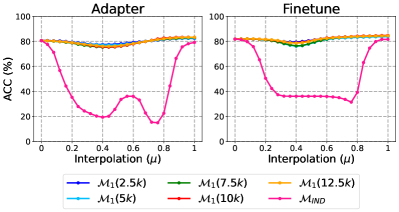
Figure 3: The performance of linear interpolations between two adapted PLMs on ChemProt. $\mu=0$ means $\mathcal{M}_{0}$, and $\mu=1$ means $\mathcal{M}_{1}(t)$ or $\mathcal{M}_{\text{IND}}$.

Results.

We illustrate the performance of the interpolations and two endpoints in Figure 3, from which we conclude that: (1) for continually pre-trained PLMs, although there exists a small performance drop in the midpoint, the interpolations generally achieve comparable performance to endpoints; (2) the connectivity does not vary much with $t$ increasing, which means within a reasonable range, the connectivity is not sensitive to longer pre-training; (3) while for independently trained PLMs, the performance drops significantly in the middle, which means the adapted weights of these PLMs cannot be linked by a high-performance linear path; (4) the above conclusions hold for both adapter and fine-tuning.

The above findings imply that when learning the same task, two continually pre-trained PLMs would probably be optimized into two minima lying in the same loss basin, or at least the optimal regions corresponding to both minima have a substantial intersection; otherwise, there should exist a significant performance drop in between.

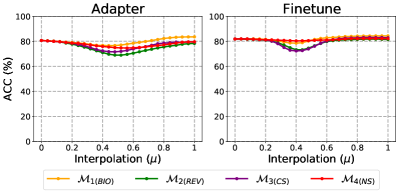
Figure 4: Linear mode connectivity between the initial $\mathcal{M}_{0}$ ($\mu=0$) and $4$ sequentially pre-trained PLMs $\{\mathcal{M}_{1},\cdots,\mathcal{M}_{4}\}$ over multiple domains ($\mu=1$).

Intuitively, the existence of a high-performance (low-loss) path between two optimal regions implies that model weights can be easily optimized from one optimal region to another without incurring a loss barrier. In this regard, it is promising to use outdated adapted weights as the initialization to find the optimal solution for the upgraded PLM, which would be explored in § 5.1. In this way, we explicitly facilitate cross-model knowledge transfer through the parameter space.

Extension to Multiple Domains.

Next, we evaluate linear mode connectivity between the initial $\mathcal{M}_{0}$ and $\mathcal{M}_{i}$ ($1\!\leq\!i\!\leq\!4$) using the task ChemProt. We derive from the results in Figure 4 that although the performance tends to drop slightly near the midpoint, the connectivity of all continually pre-trained models is still far better than independent PLMs (i.e., $\mathcal{M}_{\text{IND}}$ in Figure 3). We also observe that the performance drop between $\mathcal{M}_{0}$ and $\mathcal{M}_{2}$ is larger than $\mathcal{M}_{0}$ and $\mathcal{M}_{4}$, though $\mathcal{M}_{4}$ is trained for a longer time than $\mathcal{M}_{2}$. This means longer pre-training does not necessarily result in poorer connectivity; rather, the pre-training domain has a great impact.

4.3 Functional Similarity Analysis

The close parametric connection revealed by linear mode connectivity does not guarantee that continually pre-trained PLMs share similar functionalities when processing the text information. Following Gong et al. (2019), we explore functional similarity through the lens of attention distribution. Specifically, we investigate three continually pre-trained models ($\mathcal{M}_{0}$, $\mathcal{M}_{1}$, and $\mathcal{M}_{2}$) and fine-tune them on ChemProt to obtain adapted models ($\theta_{0}^{\mathcal{T}}$, $\theta_{1}^{\mathcal{T}}$, and $\theta_{2}^{\mathcal{T}}$). We feed the same input sampled from ChemProt to the three adapted models. Then we select attention heads from the same position (i.e., the $h$-th head in the $l$-th layer) in three models, and visualize their attention distribution. Note the selected head of $\mathcal{M}_{i+1}$ is trained from that of $\mathcal{M}_{i}$.

Figure 5: Visualization of attention heads in fine-tuned $\mathcal{M}_{0}$, $\mathcal{M}_{1}$, and $\mathcal{M}_{2}$ given the same input. For instance, “$\mathcal{L}4$ $\mathcal{H}10$” refers to the $10$-th head in the $4$-th layer. An attention head of $\mathcal{M}_{i+1}$ is trained from that of $\mathcal{M}_{i}$ in the same column. In the heatmap, the color of the $i$-th element in the $j$-th row indicates the attention value from the $j$-th token to the $i$-th token. For more visualizations (including $\mathcal{M}_{\text{IND}}$), please refer to § C.2.

From Figure 5, it is found that the attention patterns of $\mathcal{M}_{1}$ and $\mathcal{M}_{2}$ are quite similar to those of their “ancestor” $\mathcal{M}_{0}$. Such representational proximity indicates that the corresponding modules of continually pre-trained PLMs own similar functionalities. Since adapted weights play a pivotal role in stimulating PLM’s abilities and functionalities (Ding et al., 2022), such functional similarity partially explains why the outdated adapted weights can be directly applied to the upgraded PLM and achieve non-trivial performance in § 4.1.

In a nutshell, all the analyses in this section validate the close connection between continually pre-trained PLMs. Intuitively, such a connection implies that the adaptation process of these PLMs towards downstream tasks should be closely related and transferable as well, which serves as the strong basis for our recyclable tuning.

5 Methods and Experiments

Based on the findings in § 4, we propose two ways to explore the practical benefits of recyclable tuning: initialization-based method (§ 5.1) and distillation-based method (§ 5.2). The training details of this section are discussed in § D.3.

5.1 Initialization-based Recyclable Tuning

We first investigate directly using outdated weights as the initialization for tuning the upgraded PLM.

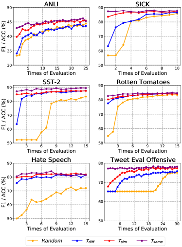
Figure 6: The performance variation in the early stage of adapter tuning for $6$ target tasks from different initialization. Different tasks are evaluated with different intervals of training steps, see § D.3 for details.

Framework.

Without loss of generality, we experiment when the initial PLM $\mathcal{M}_{0}$ is continually pre-trained on the Bio domain ($\mathcal{D}_{1}$) and upgraded to $\mathcal{M}_{1}$. Before the release of a new PLM $\mathcal{M}_{1}$, assume we have tuned $\mathcal{M}_{0}$ on N tasks $\{\mathcal{T}_{0},\cdots,\mathcal{T}_{\text{N}}\}$ and obtained the corresponding adapted weights $\{\Delta_{0}^{\mathcal{T}_{1}},\cdots,\Delta_{0}^{\mathcal{T}_{\text{N}}}\}$. When tuning $\mathcal{M}_{1}$ on a target task $\mathcal{T}_{t}$, instead of using the random initialization for tunable weights, we initialize them using $\mathcal{M}_{0}$’s adapted weights $\Delta_{0}^{\mathcal{T}_{s}}$ trained on a source task $\mathcal{T}_{s}$.

Considering that in practice, it is possible that the outdated weights of exactly the same task are not available, i.e., $\mathcal{T}_{t}\!\neq\!\mathcal{T}_{s}$. Thus we explore whether initialization from the outdated weights of a different task would suffice for our goal. Specifically, we consider three types of source tasks: (1) $\mathcal{T}_{\text{same}}$, which is the same task as the target one; (2) $\mathcal{T}_{\text{sim}}$, which denotes a task similar to $\mathcal{T}_{t}$, both $\mathcal{T}_{\text{sim}}$ and $\mathcal{T}_{t}$ typically belong to the same task type; (3) $\mathcal{T}_{\text{diff}}$, which belongs to a different task category from $\mathcal{T}_{t}$.

Settings.

We experiment with $6$ target tasks of $3$ types: (1) natural language inference: ANLI (Nie et al., 2020) and SICK (Marelli et al., 2014), (2) sentiment analysis: SST-2 (Socher et al., 2013) and Rotten Tomatoes (Pang and Lee, 2005), (3) emotion detection: Hate Speech (Davidson et al., 2017) and Tweet Eval-Offensive (Barbieri et al., 2020). The choices of $\mathcal{T}_{\text{sim}}$ and $\mathcal{T}_{\text{diff}}$ for each target task are listed in Table 12 in the appendix.

We compare the proposed initialization strategies with random initialization and record (1) the test performance variation (w.r.t. training steps) during the early stage of downstream adaptation (Figure 6), and (2) the best test performance after the adaptation converges (Table 1). For adaptation, we mainly investigate adapter tuning and leave the experiments of fine-tuning in § C.3.

Results.

The observations and corresponding conclusions are summarized as follows:

Initialization	Random	$\mathcal{T}_{\text{diff}}$	$\mathcal{T}_{\text{sim}}$	$\mathcal{T}_{\text{same}}$
ANLI	$42.5_{\pm 0.7}$	$43.7_{\pm 0.7}$	$46.2_{\pm 0.8}$	$\textbf{46.8}_{\pm 0.1}$
SICK	$87.6_{\pm 0.6}$	$\textbf{88.1}_{\pm 0.7}$	$87.7_{\pm 0.2}$	$87.9_{\pm 0.6}$
SST-2	$89.3_{\pm 0.5}$	$89.8_{\pm 0.5}$	$89.1_{\pm 0.7}$	$\textbf{90.3}_{\pm 0.5}$
R. Tomatoes	$85.3_{\pm 0.2}$	$85.2_{\pm 0.2}$	$\textbf{85.5}_{\pm 0.2}$	$84.7_{\pm 0.4}$
H. Speech	$77.2_{\pm 0.6}$	$80.1_{\pm 0.8}$	$81.9_{\pm 1.3}$	$\textbf{83.9}_{\pm 0.5}$
T. Offensive	$84.2_{\pm 0.6}$	$84.0_{\pm 0.4}$	$\textbf{84.8}_{\pm 0.2}$	$83.8_{\pm 0.1}$
Avg.	$77.7_{\pm 0.5}$	$78.5_{\pm 0.6}$	$79.2_{\pm 0.6}$	$\textbf{79.6}_{\pm 0.4}$

Table 1: The best test performance on $6$ target tasks with adapter tuning from different initialization.

(1) Faster convergence: we observe from Figure 6 that compared with the random initialization baseline, our method significantly accelerates the convergence of downstream adaptation. This suggests that the outdated weights provide a more effective initialization, allowing the PLM to be more easily optimized to the desired local optima. In practice, this method could improve the training efficiency of tuning the upgraded PLM, which saves the computations needed for adaptation.

(2) Improved task performance: we also conclude from Table 1 that after sufficient training, initialization from the outdated weights of each type of source tasks (even for $\mathcal{T}_{\text{diff}}$) could improve the final performance (up to $+1.9$ average improvement). This demonstrates that initialization serves as a valid way for cross-model knowledge transfer.

(3) Similar source tasks benefit more: comparing the results of initialization from different source tasks, we find that the improvement in both convergence and performance can be generally ranked as $\mathcal{T}_{\text{same}}\!>\!\mathcal{T}_{\text{sim}}\!>\!\mathcal{T}_{\text{diff}}$. This is because the knowledge required by more similar tasks has a greater overlap. Thus the knowledge transfer benefits more when the target task and source task are more similar. In practice, this finding expands the selection scope of source adapted weights, broadening the application scenarios for our initialization-based method.

5.2 Distillation-based Recyclable Tuning

According to Lin et al. (2021), model outputs often contain sufficient supervision that is complementary to the knowledge stored in parameters. Therefore, besides the initialization-based method, we also explore knowledge distillation (Hinton et al., 2015) to recycle the outdated weights.

Framework.

Given a task $\mathcal{T}_{j}$, assume we have optimized an outdated PLM $\mathcal{M}_{i}$ and obtained its adapted weights $\Delta_{i}^{\mathcal{T}_{j}}$. Our goal is to distill the knowledge stored in $\Delta_{i}^{\mathcal{T}_{j}}$ to optimize an updated PLM $\mathcal{M}_{i+1}$. We follow Sun et al. (2019) to construct our framework. For each data point $x$ from $\mathcal{T}_{j}$, denote $\mathcal{P}(x,\theta_{i}^{\mathcal{T}_{j}})$ as the probability distribution the adapted $\mathcal{M}_{i}$ assigns over the label space, where $\theta_{i}^{\mathcal{T}_{j}}\!=\!\theta_{i}^{0}\!\oplus\!\Delta_{i}^{\mathcal{T}_{j}}$. We minimize the KL divergence between probabilities predicted by $\mathcal{M}_{i}$ and $\mathcal{M}_{i+1}$. In addition, $\mathcal{M}_{i+1}$ mimics $\mathcal{M}_{i}$’s intermediate hidden representations of each layer. Specifically, given the same input $x$, denote $\mathbf{h}_{k}(x,\theta_{i}^{\mathcal{T}_{j}})$ and $\mathbf{h}_{k}(x,\theta_{i+1}^{\mathcal{T}_{j}})$ as the normalized hidden states of the $k$-th layer of $\mathcal{M}_{i}$ and $\mathcal{M}_{i+1}$, we minimize the mean-square loss of hidden states together with the KL divergence as follows:

$$\mathcal{L}_{\text{KD}}=\mathrm{KL}(\mathcal{P}(x,\theta_{i}^{\mathcal{T}_{j}})||\mathcal{P}(x,\theta_{i+1}^{\mathcal{T}_{j}}))+$$ (2)

$$\alpha\Sigma_{k}||\mathbf{h}_{k}(x,\theta_{i}^{\mathcal{T}_{j}})\!-\!\mathbf{h}_{k}(x,\theta_{i+1}^{\mathcal{T}_{j}})||^{2},$$

where $\alpha$ denotes a hyper-parameter. During optimization, only $\Delta_{i+1}^{\mathcal{T}_{j}}$ is tunable. Besides $\mathcal{L}_{\text{KD}}$, we also introduce the original task loss $\mathcal{L}_{\mathcal{T}_{j}}$, which is calculated using supervised training examples from task $\mathcal{T}_{j}$, with another hyper-parameter $\beta$:

$$\mathcal{L}_{\text{final}}=\beta\mathcal{L}_{\mathcal{T}_{j}}+(1-\beta)\mathcal{L}_{\text{KD}}.$$ (3)

Settings.

We consider the sequentially released PLMs $\{\mathcal{M}_{0},\cdots,\mathcal{M}_{4}\}$ as mentioned in § 3. Following Gururangan et al. (2020), we choose three tasks $\mathcal{T}_{1}$: ChemProt, $\mathcal{T}_{2}$: IMDB (Maas et al., 2011) and $\mathcal{T}_{3}$: ACL-ARC (Jurgens et al., 2018), which are relevant to domain $\mathcal{D}_{1}$, $\mathcal{D}_{2}$ and $\mathcal{D}_{3}$, respectively. We mainly consider recyclable tuning between adjacent PLMs, i.e., $\mathcal{M}_{i}$ and $\mathcal{M}_{i+1}$, and also evaluate non-adjacent PLMs (e.g., $\mathcal{M}_{i}$ and $\mathcal{M}_{i+2}$) in § C.7. For each task $\mathcal{T}_{i}$ ($i\in\{1,2,3\}$), we consider two settings:

(a) First, we recycle $\mathcal{M}_{i}$’s outdated weights to $\mathcal{M}_{i+1}$, which is denoted as $\Delta_{i}^{\mathcal{T}_{i}}\!\rightarrow\!\Delta_{i+1}^{\mathcal{T}_{i}}$. Here the evaluated task $\mathcal{T}_{i}$ is relevant to the pre-training domain $\mathcal{D}_{i}$ of the original PLM $\mathcal{M}_{i}$. During continual pre-training on $\mathcal{D}_{i+1}$, $\mathcal{M}_{i+1}$ suffers from catastrophic forgetting of $\mathcal{D}_{i}$. Hence $\mathcal{M}_{i+1}$ should perform worse on $\mathcal{T}_{i}$ than $\mathcal{M}_{i}$. In experiments, both PLMs are adapted using the same $32$-shot dataset.

Method		Teacher	$\mathcal{L}_{\text{final}}$-$\mathcal{L}_{\text{KD}}$	$\mathcal{L}_{\text{final}}$	$\mathcal{L}_{\text{final}}$+Init.
Setting (a): $\Delta_{i}^{\mathcal{T}_{i}}\!\rightarrow\!\Delta_{i+1}^{\mathcal{T}_{i}}$, $i\in\{1,2,3\}$
$\Delta_{1}^{\mathcal{T}_{1}}\!\rightarrow\!\Delta_{2}^{\mathcal{T}_{1}}$	AP	$\textbf{65.2}_{\pm 1.7}$	$58.0_{\pm 0.9}$	$62.4_{\pm 1.3}$	$63.8_{\pm 3.2}$
	FT	$\textbf{66.0}_{\pm 1.4}$	$61.4_{\pm 3.1}$	$64.5_{\pm 0.5}$	$64.7_{\pm 0.6}$
$\Delta_{2}^{\mathcal{T}_{2}}\!\rightarrow\!\Delta_{3}^{\mathcal{T}_{2}}$	AP	$\textbf{84.8}_{\pm 1.3}$	$78.3_{\pm 1.4}$	$80.7_{\pm 0.3}$	$80.8_{\pm 0.7}$
	FT	$\textbf{82.0}_{\pm 1.8}$	$76.7_{\pm 2.2}$	$79.5_{\pm 1.5}$	$79.7_{\pm 1.9}$
$\Delta_{3}^{\mathcal{T}_{3}}\!\rightarrow\!\Delta_{4}^{\mathcal{T}_{3}}$	AP	$50.6_{\pm 3.0}$	$48.2_{\pm 2.9}$	$48.0_{\pm 1.4}$	$\textbf{55.9}_{\pm 3.9}$
	FT	$52.5_{\pm 0.6}$	$51.8_{\pm 4.2}$	$54.2_{\pm 0.7}$	$\textbf{61.3}_{\pm 2.9}$
Setting (b): $\Delta_{i-1}^{\mathcal{T}_{i}}\!\rightarrow\!\Delta_{i}^{\mathcal{T}_{i}}$, $i\in\{1,2,3\}$
$\Delta_{0}^{\mathcal{T}_{1}}\!\rightarrow\!\Delta_{1}^{\mathcal{T}_{1}}$	AP	$59.1_{\pm 2.5}$	$53.1_{\pm 0.7}$	$61.4_{\pm 1.1}$	$\textbf{64.7}_{\pm 0.4}$
	FT	$61.8_{\pm 1.3}$	$56.6_{\pm 1.2}$	$59.3_{\pm 1.5}$	$\textbf{63.4}_{\pm 0.7}$
$\Delta_{1}^{\mathcal{T}_{2}}\!\rightarrow\!\Delta_{2}^{\mathcal{T}_{2}}$	AP	$83.1_{\pm 0.3}$	$84.8_{\pm 1.3}$	$86.0_{\pm 0.2}$	$\textbf{87.3}_{\pm 0.4}$
	FT	$83.3_{\pm 0.6}$	$82.0_{\pm 1.8}$	$85.5_{\pm 0.8}$	$\textbf{86.8}_{\pm 0.7}$
$\Delta_{2}^{\mathcal{T}_{3}}\!\rightarrow\!\Delta_{3}^{\mathcal{T}_{3}}$	AP	$\textbf{49.9}_{\pm 3.5}$	$49.4_{\pm 3.2}$	$49.9_{\pm 3.8}$	$49.2_{\pm 1.2}$
	FT	$54.4_{\pm 1.2}$	$49.4_{\pm 3.6}$	$50.6_{\pm 3.0}$	$\textbf{58.0}_{\pm 3.4}$

Table 2: Experiments of distillation-based recyclable tuning. For each task $\mathcal{T}_{i}$, we evaluate two settings $\Delta_{i}^{\mathcal{T}_{i}}\!\rightarrow\!\Delta_{i+1}^{\mathcal{T}_{i}}$ and $\Delta_{i-1}^{\mathcal{T}_{i}}\!\rightarrow\!\Delta_{i}^{\mathcal{T}_{i}}$. For example, $\Delta_{i}^{\mathcal{T}_{i}}\!\rightarrow\!\Delta_{i+1}^{\mathcal{T}_{i}}$ denotes distilling the knowledge of $\mathcal{M}_{i}$ to $\mathcal{M}_{i+1}$ for task $\mathcal{T}_{i}$. Here AP / FT refers to adapter / fine-tuning.

(b) Second, we evaluate the recyclable tuning from $\mathcal{M}_{i-1}$ to $\mathcal{M}_{i}$, which is denoted as $\Delta_{i-1}^{\mathcal{T}_{i}}\!\rightarrow\!\Delta_{i}^{\mathcal{T}_{i}}$. Different from setting (a), here the evaluated task $\mathcal{T}_{i}$ is relevant to the pre-training domain $\mathcal{D}_{i}$ of the newly released PLM $\mathcal{M}_{i}$. $\mathcal{M}_{i}$ performs better than $\mathcal{M}_{i-1}$ since $\mathcal{M}_{i}$ has acquired more knowledge related to $\mathcal{T}_{i}$ when learning $\mathcal{D}_{i}$. In light of this, we explore whether $\mathcal{M}_{i}$ could achieve better performance than $\mathcal{M}_{i-1}$ even when trained with fewer supervised examples. Specifically, the data size of $\mathcal{M}_{i-1}$ is set to $\{32,256,32\}$-shot for $\{\mathcal{T}_{1},\mathcal{T}_{2},\mathcal{T}_{3}\}$, and the data size of $\mathcal{M}_{i}$ is set to $\{16,32,16\}$-shot, respectively. We also evaluate our method under the zero-shot setting in § C.4.

We compare our method with utilizing only the task loss ($\mathcal{L}_{\text{final}}$-$\mathcal{L}_{\text{KD}}$) to validate the benefits of knowledge distillation. Further, we explore combining both distillation-based and initialization-based recyclable tuning ($\mathcal{L}_{\text{final}}$+Init.). This is implemented by first using the outdated weights as the initialization then tuning with $\mathcal{L}_{\text{final}}$. We also report teacher performance (Teacher) as a reference.

Results.

It can be concluded from Table 2 that: (1) compared with optimizing only the task loss ($\mathcal{L}_{\text{final}}$-$\mathcal{L}_{\text{KD}}$), distilling knowledge from the outdated weights ($\mathcal{L}_{\text{final}}$) significantly improves the performance, which shows that knowledge distillation is an effective way for recyclable tuning. (2) In general, $\mathcal{L}_{\text{final}}$+Init. leads to better performance than $\mathcal{L}_{\text{final}}$. This finding reveals that both distillation-based and initialization-based methods are complementary to each other and can be further combined to fully exploit the knowledge in outdated weights. (3) In Table 2 setting (a), $\mathcal{M}_{i+1}$ performs worse than $\mathcal{M}_{i}$ on task $\mathcal{T}_{i}$, which is because $\mathcal{M}_{i+1}$ forgets some knowledge of domain $\mathcal{D}_{i}$ when learning $\mathcal{D}_{i+1}$. However, such forgetting can be mitigated by designing better continual pre-training algorithms (Qin et al., 2022c). (4) In Table 2 setting (b), $\mathcal{M}_{i}$ outperforms $\mathcal{M}_{i-1}$ despite being trained with fewer examples. This shows that the newly acquired knowledge on domain $\mathcal{D}_{i}$ conduces to $\mathcal{M}_{i}$’s performance in $\mathcal{D}_{i}$’s relevant task $\mathcal{T}_{i}$, and improves the data efficiency. We further discuss the difference between distillation-based and initialization-based methods in appendix F.

6 Discussion

Training-free Weight Recycling.

Both methods proposed in § 5 necessitate tuning the upgraded PLM. Such a process often relies on abundant computational costs and may be infeasible practically. Given the close connections among continually pre-trained PLMs, we contend that weight recycling can be realized without training. As a preliminary exploration, we show in appendix B that it is possible to learn a cross-task generalizable projection to directly upgrade the outdated weights and make them compatible with the new PLM. Upgrading outdated weights using such a projection requires far fewer computations ($<0.002\text{\textperthousand}$) and still achieves satisfactory performance.

Downstream-compatible Continual Pre-training.

From another angle, recyclable tuning addresses the incompatibility between outdated adapted weights and the upgraded PLM from the customer perspective, analogous to the concept of forward compatibility in software engineering. In fact, the responsibility for maintaining compatibility can also be shifted to upstream suppliers during PLM upgrading (i.e., backward compatibility). Potential solutions include adding regularization terms during continual pre-training to maintain compatibility with existing adapted weights. In this way, we solve the incompatibility problem once and for all, which is more customer-friendly. However, modifying pre-training objectives may come at the cost of reduced model performance.

Broader Application Scenarios.

Although we primarily focus on recyclable tuning for one specific scenario (i.e., continual pre-training), PLMs may be subject to various types of evolution in practice. For instance, the expansion of model size (e.g., from $\text{T5}_{\texttt{BASE}}$ (Raffel et al., 2020) to $\text{T5}_{\texttt{LARGE}}$), the upgrading of model architecture (Chen et al., 2022; Lee-Thorp et al., 2022), the alteration of optimization objective (e.g., from T5 to T0 (Sanh et al., 2021) and UnifiedQA (Khashabi et al., 2020)), etc. Once the backbone infrastructure is upgraded, massive adapted weights would become outdated and potentially wasted. Hence we believe recyclable tuning in fact has broader application scenarios and we hope our findings and solutions could inspire more future research in this area.

7 Conclusion

In this paper, we formulate the task of recyclable tuning for continual pre-training. We conduct empirical analyses for this task through the lens of model compatibility, linear mode connectivity, and functional similarity. Inspired by the corresponding findings, we explore the practical benefits of recyclable tuning through parameter initialization and knowledge distillation. We also envision our setup to serve as the testbed for other topics, e.g., cross-model knowledge transfer and continual learning.

Limitations

We only experiment with two kinds of PLMs ($\text{RoBERTa}_{\texttt{BASE}}$ and $\text{RoBERTa}_{\texttt{LARGE}}$ (§ C.3 and § C.8)), leaving more diverse kinds of PLMs unexplored. While this allows us to demonstrate the effectiveness of our approach on these specific PLMs, it is important for future work to extend our problem setup to a wider range of PLMs in order to fully understand the generalizability of our findings.

Ethical Statement

In this research, we consider the following ethical issues:

• Privacy. Outdated adapted weights may contain information about the data and tasks they were trained on. Thus it is important to consider the potential privacy implications when recycling these weights. Efforts should be taken to ensure that personal or sensitive information is not disclosed during weight recycling.

• Fairness. It is crucial to guarantee that the recycling of adapted weights does not introduce biases or unfairly advantage certain tasks or domains. Thorough analysis and testing are needed to make sure that recyclable tuning does not perpetuate or amplify existing inequalities.

• Responsible AI. The responsible development and deployment of AI systems require considering the potential impacts on the environment. By improving the efficiency and sustainability of PLM adaptation, recyclable tuning contributes to the responsible development of AI systems.

• Transparency. To facilitate the responsible and ethical use of recyclable tuning, it is vital to be transparent about the methods and assumptions underlying them. We encourage future works to clearly document the conditions under which recyclable tuning is effective, as well as the potential limitations or risks.

Appendices

Appendix A Additional Backgrounds

A.1 Parameter-efficient Tuning

Conventional downstream adaptation of PLMs involves optimizing all parameters (i.e., fine-tuning), which may cause a heavy burden on the computational infrastructure and storage space. To efficiently utilize the knowledge contained in PLMs, parameter-efficient tuning (PET) is proposed, which optimizes only a few parameters and freezes the majority of parameters (Houlsby et al., 2019). Despite extensively reducing the tunable parameters, PET achieves comparable performance to fine-tuning. Besides, due to its lightweight nature, adapted weights produced by PET are easier to train, store, and share among consumers. Thus we deem PET as an essential component in our problem setup. Without loss of generality, we consider a representative PET algorithm, i.e., adapter (Houlsby et al., 2019) in this paper. Adapter inserts tunable modules into both the feed-forward module and multi-head attention module of each Transformer (Vaswani et al., 2017) layer.

A.2 Mode Connectivity

Mode connectivity measures whether two minima in the parameter space can be connected by a parametric path, where the loss (performance) remains low (high) (Garipov et al., 2018; Freeman and Bruna, 2017; Draxler et al., 2018). Such a property implies that different minima can potentially form a connected manifold in the loss landscape. For two connected minima, we can interpolate them to obtain a series of high-performance solutions. These solutions can be ensembled to achieve performance (Garipov et al., 2018) that is better than the endpoints.

Prior works in mode connectivity show that under most cases, in neural networks, there exists a non-linear low-loss path between different minima. However, only occasionally a linear low-loss path could connect different minima. Later works further contend that it is non-trivial if both minima can be connected by a linear path (Frankle et al., 2020; Mirzadeh et al., 2020). The linearity indicates that both minima may probably lie in the same loss basin (Qin et al., 2022b), which is a more favorable property and indicates a closer connection between both minima. In view of this, we focus on analyzing the linear mode connectivity in this paper.

Previous efforts were mainly spent on investigating mode connectivity for non-pre-trained models, until recently, Qin et al. (2022b) explore such property for PLMs. They focus on tuning one static base model with different adaptation strategies. Differently, we take the first step to explore mode connectivity for different backbone models (continually pre-trained PLMs) and reveal novel insights. Following Qin et al. (2022b), we present the results of task performance (e.g., accuracy) to evaluate the mode connectivity in the main paper and also report the results of task loss in appendix E.

Appendix B Training-free Weight Recycling

Although we have shown that initialization-based recyclable tuning could accelerate the convergence and improve the training efficiency, tuning the upgraded PLM still requires abundant training computations. Especially considering the massive number of tasks to handle, conducting adaptation for all of them whenever the PLM is upgraded is computationally expensive.

In this section, we explore whether we could alleviate the burden of supervised training, and directly upgrade the outdated weights at a small cost. A desired algorithm should consume significantly lower computations than that of training the new PLM from scratch. Meanwhile, this algorithm should achieve satisfactory task performance.

B.1 Framework

Inspired by Qin et al. (2021); Yi et al. (2022), we propose a training-free weight recycling method. Specifically, we learn a cross-task generalizable projection that could directly produce upgraded adapted weights for a specific task, omitting the labor of supervised training. We contend that although there exist massive downstream tasks, a large percentage of them are intrinsically similar and can be categorized into the same task type (e.g., sentiment analysis, question answering, etc.). Intuitively, the upgrading of a certain task $\mathcal{T}_{1}$ should provide a referential experience for that of a similar task $\mathcal{T}_{2}$. In view of this, we propose to make the upgrading process of $\mathcal{T}_{1}$ recyclable so that the upgrading of $\mathcal{T}_{2}$ can be achieved efficiently.

For two sequentially released PLMs $\mathcal{M}_{i}$ and $\mathcal{M}_{i+1}$, assume we have the adapted weights of $\mathcal{M}_{i}$ for both $\mathcal{T}_{1}$ and $\mathcal{T}_{2}$. We aim to recycle these adapted weights for tuning $\mathcal{M}_{i+1}$ on both tasks. As illustrated in Figure 7, our framework consists of two stages: (1) projection learning and (2) projection transferring. We learn an upgrading projection using task $\mathcal{T}_{1}$ in the first stage, and then apply (transfer) the learned projection to task $\mathcal{T}_{2}$ in the second stage. Note the first stage requires training while the second stage is training-free. Next, we introduce the details of the two stages.

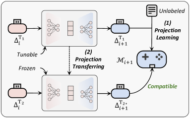
Figure 7: Illustration of our training-free weight recycling algorithm. We learn a cross-task generalizable projection (i.e., the projection learning stage) that could directly upgrade outdated adapted weights (i.e., the projection transferring stage).

Projection Learning.

Instead of directly optimizing the parameters in $\Delta_{i+1}^{\mathcal{T}_{1}}$, we learn a low-rank decomposition $\Delta_{i+1}^{\mathcal{T}_{1}}=\texttt{Proj}(\Delta_{i}^{\mathcal{T}_{1}})$ as follows:

$$\texttt{Proj}^{*}_{i\rightarrow i+1}=\operatorname*{arg\,min}_{\texttt{Proj}}\mathcal{L}(\texttt{Proj}(\Delta_{i}^{\mathcal{T}_{1}})),$$

where $\texttt{Proj}\!=\!\texttt{Proj}_{\uparrow}\times\texttt{Proj}_{\downarrow}$. Denote $d$ as a low-dimensional bottleneck dimension, $\texttt{Proj}_{\downarrow}$ projects the dimension of $\Delta_{i}^{\mathcal{T}_{1}}$ to $d$, i.e., $\texttt{Proj}_{\downarrow}(\Delta_{i}^{\mathcal{T}_{1}})\!\in\!\mathbb{R}^{d}$. Then $\texttt{Proj}_{\uparrow}$ projects the dimension from $d$ back to $|\Delta_{i}^{\mathcal{T}_{1}}|$, i.e., $\texttt{Proj}_{\uparrow}(\texttt{Proj}_{\downarrow}(\Delta_{i}^{\mathcal{T}_{1}}))\!\in\!\mathbb{R}^{|\Delta_{i}^{\mathcal{T}_{1}}|}$. Either $\texttt{Proj}_{\uparrow}$ or $\texttt{Proj}_{\downarrow}$ is implemented by a $2$-layer MLP. During training, $\Delta_{i}^{\mathcal{T}_{1}}$ is kept frozen and only the parameters in Proj are tuned. Note the dimensions of $\Delta_{i}^{\mathcal{T}_{1}}$ and $\Delta_{i+1}^{\mathcal{T}_{1}}$ are the same, i.e., $|\Delta_{i}^{\mathcal{T}_{1}}|\!=\!|\Delta_{i+1}^{\mathcal{T}_{1}}|$. $\texttt{Proj}(\Delta_{i}^{\mathcal{T}_{1}})$ is then applied to the upgraded PLM $\mathcal{M}_{i+1}$ to compute the loss $\mathcal{L}$.

Projection Transferring.

When upgrading the outdated weights of a similar task $\mathcal{T}_{2}$, we directly apply the projection $\texttt{Proj}^{*}_{i\rightarrow i+1}$ learned on $\mathcal{T}_{1}$ to $\Delta_{i}^{\mathcal{T}_{2}}$ and obtain the approximated updated weights $\Delta_{i+1}^{\mathcal{T}_{2*}}$:

$$\Delta_{i+1}^{\mathcal{T}_{2*}}=\texttt{Proj}^{*}_{i\rightarrow i+1}(\Delta_{i}^{\mathcal{T}_{2}}).$$

We formulate the downstream tuning as prompt learning (Schick and Schütze, 2021), instead of introducing additional classification heads for different tasks. Hence the number of parameters in $\Delta_{i}^{\mathcal{T}_{1}}$ and $\Delta_{i}^{\mathcal{T}_{2}}$ is the same, i.e., $|\Delta_{i}^{\mathcal{T}_{1}}|=|\Delta_{i}^{\mathcal{T}_{2}}|$. Note that only applying the projection to compute the upgraded weights consumes very limited computations (see Figure 8), hence we significantly reduce the computations of learning $\Delta_{i+1}^{\mathcal{T}_{2}}$, compared with the conventional tuning-based method.

Besides, since the projection Proj comprises an integral multiple ($d\times$) of $\Delta_{i}^{\mathcal{T}_{1}}$’s parameters, our solution is only feasible for parameter-efficient tuning. While for fine-tuning, it is computationally intractable to train the projection due to the tremendous size of parameters in $\Delta_{i}^{\mathcal{T}_{1}}$ and Proj. Being the first attempt in this research direction, we leave corresponding explorations for fine-tuning as future work.

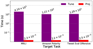
Figure 8: Time needed for upgrading outdated weights on different target tasks. Our proposed training-free weight recycling method (Proj) consumes $<0.002\text{\textperthousand}$ computations than the conventional tuning-based method (Tune).

B.2 Experiments

Settings.

We mainly evaluate $\mathcal{M}_{1}$ and $\mathcal{M}_{2}$ as defined in § 3. We choose a series of NLP tasks and categorize them into $3$ classes: (1) natural language inference: MNLI, SICK, ANLI, QNLI (Rajpurkar et al., 2016), and WNLI (Faruqui and Das, 2018), (2) sentiment analysis: SST-2, Amazon Polarity (McAuley and Leskovec, 2013), and Rotten Tomatoes, (3) emotion detection: Hate Speech, Tweet Eval-Offensive, Tweet Eval-Hate, Tweet Eval-Abortion, Tweet Eval-Feminist, and Tweet Eval-Atheism from Barbieri et al. (2020). We partition the tasks belonging to the same category into source task $\mathcal{T}_{1}$ and target task $\mathcal{T}_{2}$ (see Table 3), and learn the projection Proj on the source task.

We consider the zero-shot setting for the first stage (projection learning) and use the knowledge distillation loss function $\mathcal{L}_{\text{KD}}$. Here the teacher model weights are the adapted $\mathcal{M}_{1}$, and the student model weights are obtained by applying $\texttt{Proj}(\Delta_{1}^{\mathcal{T}_{1}})$ to the pre-trained weights of $\mathcal{M}_{2}$. For the unlabeled corpus used for distillation, we evaluate both the target task data (denoted as $\mathcal{L}_{\text{KD}}^{\mathcal{T}}$) and Wikipedia corpora ($\mathcal{L}_{\text{KD}}^{\text{wiki}}$). Note for the former, we only use the input $x$ and discard the corresponding label $y$ (i.e., the zero-shot setting). The former can be seen as the upper bound for the latter since the data format of the latter may not be compatible with the target task. After that, we directly utilize the learned projection to upgrade the outdated weights of similar target tasks.

Baselines.

We consider demonstration learning (Brown et al., 2020) as the baseline, which integrates a few labeled examples into the input text as additional context. The PLM directly performs inference on the test set without incurring any training. For reference, we also report the performance when $\mathcal{M}_{2}$ is adapted using the full dataset (FD) and the $32$-shot dataset (FS). Instead, our method requires no labeled data.

Source	Target	$\mathcal{L}_{\text{KD}}^{\mathcal{T}}$	$\mathcal{L}_{\text{KD}}^{\text{wiki}}$	Demo.	FD	FS
MNLI	SICK	$75.2$	$74.3$	$60.5$	88.1	$78.0$
ANLI	MNLI	$65.2$	$43.7$	$46.1$	79.9	$41.7$
QNLI	WNLI	72.2	$58.3$	$55.6$	$55.6$	$50.0$
SST-2	A. Polarity	$95.0$	$94.0$	$81.8$	95.8	$94.1$
SST-2	R. Tomatoes	87.8	$84.7$	$71.4$	$87.4$	$78.7$
H. Speech	T. Offensive	$77.1$	$74.5$	$63.5$	84.5	$71.4$
H. Speech	T. Hate	62.4	$59.1$	$50.7$	$52.7$	$49.2$
Abortion	Feminist	$63.5$	64.6	$47.7$	$59.0$	$49.5$
Abortion	Atheism	$71.8$	$70.0$	$51.4$	74.6	$65.0$

Table 3: Performance evaluation for our training-free upgrading algorithm. We distill the knowledge of outdated weights using both unlabeled task data ($\mathcal{L}_{\text{KD}}^{\mathcal{T}}$) and Wikipedia ($\mathcal{L}_{\text{KD}}^{\text{wiki}}$). We also report the performance of directly tuning the upgraded PLM using the full dataset (FD) or $32$-shot data (FS), and the demonstration learning baseline (Demo.).

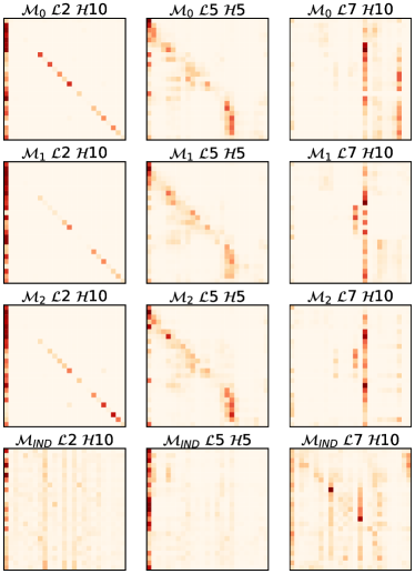
Figure 9: More attention visualization of attention heads in fine-tuned $\mathcal{M}_{0}$, $\mathcal{M}_{1}$, and $\mathcal{M}_{2}$ given the same input. Apart from the above PLMs, we also present the attention pattern of an independently trained PLM $\mathcal{M}_{\text{IND}}$.

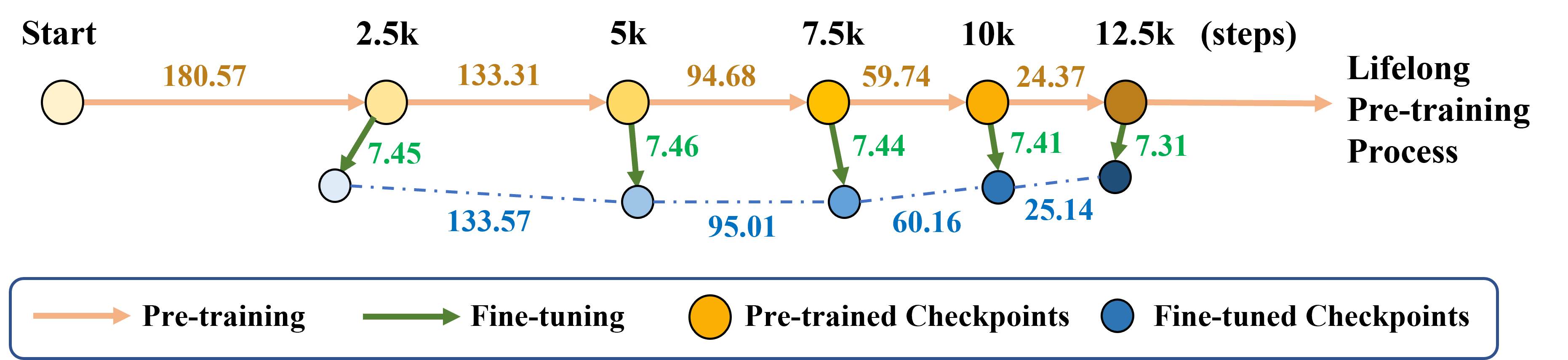
Figure 10: Euclidean distance of continually pre-trained PLMs and their adapted weights. During pre-training, we save the checkpoint for every $2.5$k steps and fine-tune each checkpoint on the task ChemProt.

Efficiency Evaluation.

We compare the computational costs needed for our training-free method and the conventional tuning-based method in Figure 8. For the former, we record the time needed in projection transferring (i.e., computing the upgraded weights $\Delta_{i+1}^{\mathcal{T}_{2*}}$). For the latter, we record the training time needed until an adaptation converges. It can be derived that our method requires significantly fewer computations, which demonstrates its efficiency. In practice, such a projection can be trained once and for all. As long as we have obtained the projection, we can directly upgrade potentially massive outdated weights in an efficient manner, and the computations involved during projection learning can be neglected. Although currently we only support projection transferring for a similar target task that belongs to the same category of the source task, we expect future work to explore how to train a universal projection that could be applied to an arbitrary task.

Performance Evaluation.

The results are shown in Table 3, from which we find that: (1) our method generally outperforms the demonstration baseline, and could surpass the supervised performance (FD and FS) under certain cases, despite not using any labeled data. Hence, besides being computationally efficient, our method achieves satisfactory performance in general. This also validates our intuition that for continually pre-trained PLMs, the upgrading of a specific task could provide referential experience for similar tasks; (2) using the task data ($\mathcal{L}_{\text{KD}}^{\mathcal{T}}$) for distillation generally performs better than using Wikipedia ($\mathcal{L}_{\text{KD}}^{\text{wiki}}$), showing the importance of proper data distribution used for knowledge distillation.

Appendix C Additional Experiments and Analyses

C.1 Euclidean Distance Analysis

We report the Euclidean distance of continually pre-trained PLMs and the corresponding adapted models. We evaluate when the official $\text{RoBERTa}_{\texttt{BASE}}$ is adapted on the Bio domain for $12.5$k steps following the settings in § 3. We save the checkpoint for every $2.5$k steps. For each checkpoint $\mathcal{M}_{1}(t)$, denote its weights as $\theta_{1}^{0}(t)$, we fine-tune it on ChemProt to obtain its adapted weights $\Delta_{1}^{\mathcal{T}}(t)$, where $|\Delta_{1}^{\mathcal{T}}(t)|=|\theta_{1}^{0}(t)|$. The resultant model weights are $\theta_{1}^{\mathcal{T}}(t)=\theta_{1}^{0}(t)\oplus\Delta_{1}^{\mathcal{T}}(t)$.

Initialization	Random	$\mathcal{T}_{\text{diff}}$	$\mathcal{T}_{\text{sim}}$	$\mathcal{T}_{\text{same}}$
ANLI	$47.4_{\pm 0.9}$	$46.3_{\pm 1.1}$	$\textbf{49.6}_{\pm 1.1}$	$48.8_{\pm 0.9}$
SICK	$88.8_{\pm 0.2}$	$88.8_{\pm 0.3}$	$89.4_{\pm 0.4}$	$\textbf{89.5}_{\pm 0.2}$
H. Speech	$79.9_{\pm 3.1}$	$\textbf{82.4}_{\pm 0.9}$	$78.4_{\pm 2.0}$	$81.1_{\pm 2.6}$
Avg.	$72.0_{\pm 1.4}$	$72.5_{\pm 0.8}$	$72.5_{\pm 1.2}$	$\textbf{73.1}_{\pm 1.2}$

Table 4: The best test performance on $3$ target tasks with fine-tuning from different initialization using $\text{RoBERTa}_{\texttt{BASE}}$.

Given two continually pre-trained models $\mathcal{M}_{1}(t)$ and $\mathcal{M}_{1}(t^{\prime})$, where $t^{\prime}\!=\!t+2.5\text{k}$, we flatten their pre-trained weights $\theta_{1}^{0}(t)$ and $\theta_{1}^{0}(t^{\prime})$, and calculate their $L$-2 norm: $||\theta_{1}^{0}(t^{\prime})-\theta_{1}^{0}(t)||$. In addition, we also calculate the $L$-2 norm of flattened adapted weights ($||\Delta_{1}^{\mathcal{T}}(t)||$ / $||\Delta_{1}^{\mathcal{T}}(t^{\prime})||$) and distance between adapted PLMs ($||\theta_{1}^{\mathcal{T}}(t^{\prime})-\theta_{1}^{\mathcal{T}}(t)||$). We illustrate the results in Figure 10 and find that: (1) $||\theta_{1}^{0}(t^{\prime})-\theta_{1}^{0}(t)||$ / $||\theta_{1}^{\mathcal{T}}(t^{\prime})-\theta_{1}^{\mathcal{T}}(t)||$ gradually decreases with $t$ increasing. This is mainly because the learning rates are warmed up for the first $6\%$ steps, and the learning rate starts to decrease at the $0.75$k-th step, which means the PLM gradually moves slower in the parameter space; (2) the parameter change caused by downstream adaptation (i.e., $||\Delta_{1}^{\mathcal{T}}(t)||$ / $||\Delta_{1}^{\mathcal{T}}(t^{\prime})||$) is far smaller than that brought by continual pre-training ($||\theta_{1}^{0}(t^{\prime})-\theta_{1}^{0}(t)||$). This is because downstream adaptation converges shortly. After convergence, the model parameters generally stay in a specific optimal region. While continual pre-training constantly pushes the model weights away from the previous checkpoints in the parameter space. Another reason is that continual pre-training uses a large batch $2048$, while downstream adaptation often uses a much smaller batch size (e.g., $16$).

C.2 More Visualization for Functional Similarity Analysis

In the main paper (Figure 5), we visualize three different attention heads of $\mathcal{M}_{0}$, $\mathcal{M}_{1}$, and $\mathcal{M}_{2}$. In this section, we present more visualizations to further support our claim. We also visualize the attention pattern of an independently trained PLM $\mathcal{M}_{\text{IND}}$. The results in Figure 9 again demonstrate our claim that continually pre-trained PLMs exhibit similar attention patterns, which independently trained PLMs do not have.

C.3 Initialization-based Recyclable Tuning for Fine-tuning and $\text{RoBERTa}_{\texttt{LARGE}}$

In § 5.1, we mainly evaluate initialization-based recyclable tuning using $\text{RoBERTa}_{\texttt{BASE}}$ and adapter tuning. Here we extend the experiments to either fine-tuning (Table 4) or $\text{RoBERTa}_{\texttt{LARGE}}$ (Table 5). We choose $3$ tasks in Table 1 and follow most of the settings. From Table 4 and Table 5, we find that the main conclusions are generally consistent with those mentioned in the main paper. This implies that the initialization-based method can be applied to different tuning methods and PLMs.

Initialization	Random	$\mathcal{T}_{\text{diff}}$	$\mathcal{T}_{\text{sim}}$	$\mathcal{T}_{\text{same}}$
ANLI	$56.6_{\pm 0.3}$	$57.0_{\pm 0.2}$	$\textbf{61.0}_{\pm 0.4}$	$59.9_{\pm 0.5}$
SICK	$89.8_{\pm 0.3}$	$89.6_{\pm 0.1}$	$\textbf{91.5}_{\pm 0.3}$	$90.6_{\pm 0.4}$
H. Speech	$84.7_{\pm 1.3}$	$82.1_{\pm 0.5}$	$83.6_{\pm 0.7}$	$\textbf{85.3}_{\pm 0.4}$
Avg.	$77.0_{\pm 0.6}$	$76.2_{\pm 0.3}$	$\textbf{78.7}_{\pm 0.5}$	$78.6_{\pm 0.4}$

Table 5: The best test performance on $3$ target tasks with adapter tuning from different initialization using $\text{RoBERTa}_{\texttt{LARGE}}$.

C.4 Distillation-based Recyclable Tuning under the Zero-shot Setting

We extend our distillation-based recyclable tuning to the zero-shot setting where there is no labeled data for tuning the upgraded PLM. We show that it is able to utilize unlabeled raw corpora to distill the knowledge of outdated weights. Specifically, we remove the task loss $\mathcal{L}_{\mathcal{T}}$ in $\mathcal{L}_{\text{final}}$ and only retain $\mathcal{L}_{\text{KD}}$. Instead of using supervised examples, we sample unlabeled data $x$ from Wikipedia to compute $\mathcal{L}_{\text{KD}}$. We evaluate recyclable tuning between $\mathcal{M}_{1}$ and $\mathcal{M}_{2}$ and choose $4$ downstream tasks, i.e., ChemProt, IMDB, SST-2, and MNLI. For each task, the outdated weights of $\mathcal{M}_{1}$ are obtained with the full dataset, and our goal is to distill their knowledge and optimize $\mathcal{M}_{2}$’s weights.

Two training-free baselines are considered: (1) manual prompting (Schick and Schütze, 2021), which restructures the input into templates by inserting prompts, and (2) demonstration learning, which has been introduced in § B.2. For both baselines, the PLM directly performs inference on the test set without incurring any training. Moreover, we also evaluate the performance when knowledge distillation is combined with the initialization-based method.

Task	ChemProt		IMDB		SST-2		MNLI
Prompt	$8.9$		$74.4$		$81.2$		$44.4$
Demo.	$9.8$		$78.1$		$84.4$		$47.1$
Method	AP	FT	AP	FT	AP	FT	AP	FT
$\mathcal{L}_{\text{KD}}$	$63.8$	$67.4$	$89.4$	$88.6$	$90.6$	$92.0$	$56.5$	$78.3$
$\mathcal{L}_{\text{KD}}$+Init.	73.5	76.0	90.3	90.4	92.5	92.5	76.0	78.3

Table 6: Zero-shot experiments for distillation-based recyclable tuning between $\mathcal{M}_{1}$ and $\mathcal{M}_{2}$. The outdated weights of $\mathcal{M}_{1}$ are trained using the full dataset. Both manual prompting (Prompt) and demonstration learning (Demo.) are compared as the baseline.

We list the results in Table 6, from which it can be derived that: (1) our method surpasses manual prompting and demonstration learning by a large margin, which shows the benefits of recycling outdated adapted weights in the zero-shot setting; (2) initializing tunable weights with the outdated weights could further improve the performance of $\mathcal{L}_{\text{KD}}$, which again demonstrates that both initialization-based and distillation-based methods are complementary to each other.

C.5 Interpolation Distillation

Traditional knowledge distillation frameworks have no assumptions about the parametric connection between the teacher and the student, and resort to pulling closer their predictions ($\mathcal{P}$) or inner representations ($\mathbf{h}$). As we have shown in the main paper, continually pre-trained PLMs are guaranteed with close parametric connections. Therefore, traditional knowledge distillation methods may fail to exploit the parametric knowledge contained in the teacher model’s parameters. Here we explore another way for more effective distillation-based recyclable tuning under our setting.

Method		$\mathcal{L}_{\text{final}}$-$\mathcal{L}_{\text{KD}}$	$\mathcal{L}_{\text{final}}$	$\mathcal{L}_{\text{final}}$+Init.	$\mathcal{L}_{\text{ITP}}$
Setting (a): $\Delta_{i}^{\mathcal{T}_{i}}\!\rightarrow\!\Delta_{i+1}^{\mathcal{T}_{i}}$, $i\in\{1,2,3\}$
$\Delta_{1}^{\mathcal{T}_{1}}\!\rightarrow\!\Delta_{2}^{\mathcal{T}_{1}}$	AP	$58.0_{\pm 0.9}$	$62.4_{\pm 1.3}$	$63.8_{\pm 3.2}$	$\textbf{64.4}_{\pm 1.9}$
	FT	$61.4_{\pm 3.1}$	$64.5_{\pm 0.5}$	$64.7_{\pm 0.6}$	$\textbf{64.8}_{\pm 0.8}$
$\Delta_{2}^{\mathcal{T}_{2}}\!\rightarrow\!\Delta_{3}^{\mathcal{T}_{2}}$	AP	$78.3_{\pm 1.4}$	$80.7_{\pm 0.3}$	$80.8_{\pm 0.7}$	$\textbf{80.9}_{\pm 0.3}$
	FT	$76.7_{\pm 2.2}$	$79.5_{\pm 1.5}$	$79.7_{\pm 1.9}$	$\textbf{80.2}_{\pm 0.3}$
$\Delta_{3}^{\mathcal{T}_{3}}\!\rightarrow\!\Delta_{4}^{\mathcal{T}_{3}}$	AP	$48.2_{\pm 2.9}$	$48.0_{\pm 1.4}$	$\textbf{55.9}_{\pm 3.9}$	$51.3_{\pm 3.2}$
	FT	$51.8_{\pm 4.2}$	$54.2_{\pm 0.7}$	$\textbf{61.4}_{\pm 2.9}$	$55.6_{\pm 3.2}$
Setting (b): $\Delta_{i-1}^{\mathcal{T}_{i}}\!\rightarrow\!\Delta_{i}^{\mathcal{T}_{i}}$, $i\in\{1,2,3\}$
$\Delta_{0}^{\mathcal{T}_{1}}\!\rightarrow\!\Delta_{1}^{\mathcal{T}_{1}}$	AP	$53.1_{\pm 0.7}$	$61.4_{\pm 1.1}$	$\textbf{64.7}_{\pm 0.4}$	$62.3_{\pm 1.4}$
	FT	$56.6_{\pm 1.2}$	$59.3_{\pm 1.5}$	$\textbf{63.4}_{\pm 0.7}$	$62.8_{\pm 1.2}$
$\Delta_{1}^{\mathcal{T}_{2}}\!\rightarrow\!\Delta_{2}^{\mathcal{T}_{2}}$	AP	$84.8_{\pm 1.3}$	$86.0_{\pm 0.2}$	$\textbf{87.3}_{\pm 0.4}$	$86.2_{\pm 0.4}$
	FT	$82.0_{\pm 1.8}$	$85.5_{\pm 0.8}$	$\textbf{86.8}_{\pm 0.7}$	$85.7_{\pm 1.0}$
$\Delta_{2}^{\mathcal{T}_{3}}\!\rightarrow\!\Delta_{3}^{\mathcal{T}_{3}}$	AP	$49.4_{\pm 3.2}$	$49.9_{\pm 3.8}$	$49.2_{\pm 1.2}$	$\textbf{50.4}_{\pm 3.3}$
	FT	$49.4_{\pm 3.6}$	$50.6_{\pm 3.0}$	$\textbf{58.0}_{\pm 3.4}$	$86.2_{\pm 0.4}$

Table 7: Performance of interpolation distillation. We follow the settings in § 5.2. The results of $\mathcal{L}_{\text{final}}$-$\mathcal{L}_{\text{KD}}$, $\mathcal{L}_{\text{final}}$, and $\mathcal{L}_{\text{final}}$+Init. are borrowed from Table 2.

Framework.

Inspired by MC-SGD (Mirzadeh et al., 2020), we propose an interpolation distillation technique to fully exploit the parametric knowledge contained in outdated adapted weights. Specifically, for recyclable tuning between $\mathcal{M}_{i}$ and $\mathcal{M}_{i+1}$, instead of optimizing the overall loss function using the only endpoint checkpoint ($\theta_{i+1}^{\mathcal{L}_{j}}=\theta_{i+1}^{0}\oplus\Delta_{i+1}^{\mathcal{T}_{j}}$) for task $\mathcal{T}_{j}$, we linearly interpolate $\theta_{i}^{\mathcal{L}_{j}}$ and $\theta_{i+1}^{\mathcal{L}_{j}}$ to obtain a series of model checkpoints: $\theta(\mu)=(1-\mu)\theta_{i}^{\mathcal{L}_{j}}+\mu\theta_{i+1}^{\mathcal{L}_{j}}$. After that, we feed data into $\theta(\mu)$ and minimize the corresponding loss together with $\mathcal{L}(\theta_{i+1}^{\mathcal{L}_{j}})$:

$$\mathcal{L}_{\text{ITP}}(\Delta_{i+1}^{\mathcal{T}_{j}})=\mathcal{L}(\theta_{i+1}^{\mathcal{L}_{j}})\!+\!\gamma\!\!\!\!\!\!\sum_{\mu\in\{\frac{1}{N_{\mu}},\cdots,\frac{N_{\mu}-1}{N_{\mu}}\}}\!\!\!\!\!\!\mathcal{L}(\theta(\mu)),$$

where $\gamma$ is a hyper-parameter, and $N_{\mu}$ denotes a constant integer. In practice, we found a small $N_{\mu}$ (e.g., $2$) already achieves satisfying performance. During optimization, only $\Delta_{i+1}^{\mathcal{T}_{j}}$ is tuned by receiving gradients from both $\mathcal{L}(\theta_{i+1}^{j})$ and $\mathcal{L}(\theta(\mu))$.

Experiments.

We follow most of the settings in § 5.2 and evaluate the performance of interpolation distillation. We compare it with the results of $\mathcal{L}_{\text{final}}$-$\mathcal{L}_{\text{KD}}$, $\mathcal{L}_{\text{final}}$, and $\mathcal{L}_{\text{final}}$+Init.. All results are shown in Table 7, from which we observe that the interpolation distillation method ($\mathcal{L}_{\text{ITP}}$) generally outperforms the vanilla distillation ($\mathcal{L}_{\text{final}}$), and could surpass $\mathcal{L}_{\text{final}}$+Init. in certain cases. This shows that interpolation distillation successfully exploits the parametric knowledge contained in the outdated adapted weights, and serves as an improved method for the distillation-based method.

Method		$\mathcal{L}_{\text{final}}$-$\mathcal{L}_{\text{KD}}$	$\mathcal{L}_{\text{final}}$	$\mathcal{L}_{\text{ITP}}$	$\mathcal{L}_{\text{final}}$+Init.
Setting: full-data teacher
$\Delta_{1}^{\mathcal{T}_{1}}\!\rightarrow\!\Delta_{2}^{\mathcal{T}_{1}}$	AP	$58.0_{\pm 0.9}$	$71.3_{\pm 1.9}$	$\textbf{76.8}_{\pm 0.6}$	$73.1_{\pm 1.3}$
	FT	$61.4_{\pm 3.1}$	$70.7_{\pm 1.5}$	$74.4_{\pm 0.8}$	$\textbf{76.2}_{\pm 0.5}$
$\Delta_{2}^{\mathcal{T}_{2}}\!\rightarrow\!\Delta_{3}^{\mathcal{T}_{2}}$	AP	$78.3_{\pm 1.4}$	$84.3_{\pm 0.5}$	$84.7_{\pm 0.3}$	$\textbf{86.7}_{\pm 0.5}$
	FT	$76.7_{\pm 2.2}$	$83.5_{\pm 0.9}$	$84.2_{\pm 0.1}$	$\textbf{87.3}_{\pm 0.4}$
$\Delta_{3}^{\mathcal{T}_{3}}\!\rightarrow\!\Delta_{4}^{\mathcal{T}_{3}}$	AP	$48.2_{\pm 2.9}$	$66.7_{\pm 0.9}$	$67.4_{\pm 0.7}$	$\textbf{68.3}_{\pm 2.6}$
	FT	$51.8_{\pm 4.2}$	$62.8_{\pm 3.0}$	$65.2_{\pm 1.4}$	$\textbf{69.8}_{\pm 1.8}$

Table 8: Experiments on $\text{RoBERTa}_{\texttt{BASE}}$ when teacher models are adapted with the full-size dataset. Other settings are kept the same with Table 2 setting (a).

C.6 Effects of Teacher Model Capability for Distillation-based Recyclable Tuning

For experiments of setting (a) in distillation-based recyclable tuning (§ 5.2), the teacher model is trained with the same $32$-shot dataset as the student model. Here we explore whether a teacher model with stronger capabilities would conduce to the student’s performance. Specifically, keeping all the other settings the same, we change the teacher model’s data to the full-data size. The new results are placed in Table 8, from which we conclude that: (1) our methods ($\mathcal{L}_{\text{final}}$, $\mathcal{L}_{\text{ITP}}$, and $\mathcal{L}_{\text{final}}$+Init.) still outperform the baseline without knowledge distillation ($\mathcal{L}_{\text{final}}$-$\mathcal{L}_{\text{KD}}$); (2) comparing the student’s performance in Table 8 and Table 2 setting (a), we find through learning from a more powerful teacher, the student’s performance is improved as well.

C.7 Experiments on Non-adjacent PLMs

Method		$\mathcal{L}_{\text{final}}$-$\mathcal{L}_{\text{KD}}$	$\mathcal{L}_{\text{final}}$	$\mathcal{L}_{\text{ITP}}$	$\mathcal{L}_{\text{final}}$+Init.
Few-shot teacher
$\Delta_{1}^{\mathcal{T}_{1}}\!\rightarrow\!\Delta_{3}^{\mathcal{T}_{1}}$	AP	$60.5_{\pm 2.1}$	$66.3_{\pm 1.5}$	$\textbf{67.5}_{\pm 1.7}$	$67.2_{\pm 1.5}$
	FT	$61.9_{\pm 1.3}$	$64.7_{\pm 0.9}$	$64.8_{\pm 0.8}$	$\textbf{65.4}_{\pm 1.3}$
$\Delta_{1}^{\mathcal{T}_{1}}\!\rightarrow\!\Delta_{4}^{\mathcal{T}_{1}}$	AP	$56.6_{\pm 1.1}$	$57.9_{\pm 1.5}$	$\textbf{65.3}_{\pm 1.7}$	$64.9_{\pm 3.6}$
	FT	$59.7_{\pm 2.3}$	$62.9_{\pm 2.4}$	$64.4_{\pm 0.5}$	$\textbf{65.1}_{\pm 2.2}$
Full-data teacher
$\Delta_{1}^{\mathcal{T}_{1}}\!\rightarrow\!\Delta_{3}^{\mathcal{T}_{1}}$	AP	$60.5_{\pm 2.1}$	$74.2_{\pm 0.9}$	$77.8_{\pm 0.6}$	$\textbf{78.0}_{\pm 0.5}$
	FT	$61.9_{\pm 1.3}$	$70.9_{\pm 0.5}$	$73.3_{\pm 1.0}$	$\textbf{77.3}_{\pm 0.7}$
$\Delta_{1}^{\mathcal{T}_{1}}\!\rightarrow\!\Delta_{4}^{\mathcal{T}_{1}}$	AP	$56.6_{\pm 1.1}$	$68.6_{\pm 0.7}$	$75.6_{\pm 0.7}$	$\textbf{76.7}_{\pm 0.1}$
	FT	$59.7_{\pm 2.3}$	$69.8_{\pm 0.5}$	$74.0_{\pm 0.5}$	$\textbf{76.0}_{\pm 0.8}$

Table 9: Experiments for distillation-based recyclable tuning between non-adjacent PLMs, i.e., ($\mathcal{M}_{1}$, $\mathcal{M}_{3}$) and ($\mathcal{M}_{1}$, $\mathcal{M}_{4}$). We follow the setting (a) in § 5.2. The teacher model is trained using either the $32$-shot data or the full data. The student model is trained using the $32$-shot data.

For most of the experiments, we mainly focus on recyclable tuning between adjacent PLMs. We contend that the proposed methods should also work for non-adjacent PLMs since they are still guaranteed with close connections. To demonstrate this, we take the distillation-based recyclable tuning as an example. Specifically, we evaluate the distillation-based recyclable tuning between ($\mathcal{M}_{1}$, $\mathcal{M}_{3}$) and ($\mathcal{M}_{1}$, $\mathcal{M}_{4}$) using $\mathcal{T}_{1}$, and largely follow the settings in § 5.2. We choose setting (a) in § 5.2, and the only difference is that the teacher model $\mathcal{M}_{1}$ is trained either using the $32$-shot dataset (dubbed as few-shot teacher) or the full dataset (dubbed as full-data teacher). While the student model is trained using the $32$-shot dataset. In this way, we could understand the role of the teacher model in knowledge distillation.

The results are placed in Table 9, from which we find that: (1) introducing knowledge distillation ($\mathcal{L}_{\text{final}}$) improves the performance than only using task loss ($\mathcal{L}_{\text{final}}$-$\mathcal{L}_{\text{KD}}$) and (2) introducing the parametric knowledge either through interpolation distillation ($\mathcal{L}_{\text{ITP}}$) or weight initialization ($\mathcal{L}_{\text{final}}$+Init.) could further improve the task performance. Both conclusions are aligned with those obtained on adjacent PLMs. This demonstrates our claim that our recyclable tuning is not limited to adjacent PLMs, but also non-adjacent ones. Finally, we observe that the student performance when the teacher is trained using full data is much better, which shows the benefits of learning from a more advanced teacher.

C.8 Distillation-based Recyclable Tuning Experiments using $\text{RoBERTa}_{\texttt{LARGE}}$

Method		$\mathcal{L}_{\text{final}}$-$\mathcal{L}_{\text{KD}}$	$\mathcal{L}_{\text{final}}$	$\mathcal{L}_{\text{ITP}}$	$\mathcal{L}_{\text{final}}$+Init.
Few-shot teacher
$\Delta_{1}^{\mathcal{T}_{1}}\!\rightarrow\!\Delta_{2}^{\mathcal{T}_{1}}$	AP	$64.6_{\pm 1.2}$	$\textbf{69.3}_{\pm 0.8}$	$70.2_{\pm 0.1}$	$69.2_{\pm 1.1}$
	FT	$64.7_{\pm 2.7}$	$70.3_{\pm 1.6}$	$70.9_{\pm 2.0}$	$\textbf{72.5}_{\pm 1.1}$
Full-data teacher
$\Delta_{1}^{\mathcal{T}_{1}}\!\rightarrow\!\Delta_{2}^{\mathcal{T}_{1}}$	AP	$64.6_{\pm 1.2}$	$78.8_{\pm 0.6}$	$\textbf{82.8}_{\pm 0.3}$	$82.4_{\pm 0.5}$
	FT	$64.7_{\pm 2.7}$	$76.9_{\pm 0.5}$	$79.8_{\pm 1.0}$	$\textbf{82.1}_{\pm 0.3}$

Table 10: Experiments of distillation-based recyclable tuning for $\text{RoBERTa}_{\texttt{LARGE}}$ ($\mathcal{M}_{1}$, $\mathcal{M}_{2}$). We follow the setting (a) in § 5.2. The teacher model is trained using either the $32$-shot data or the full data. The student model is trained using the $32$-shot data.

Previous experiments for distillation-based recyclable tuning are based on $\text{RoBERTa}_{\texttt{BASE}}$, now we turn to $\text{RoBERTa}_{\texttt{LARGE}}$ to show that our proposed methods are model-agnostic. We experiment with $\mathcal{M}_{1}$ and $\mathcal{M}_{2}$ using the task ChemProt. Other settings are kept the same as those in § C.7. In Table 10, we show that the results are generally aligned with our conclusions before. These results also reflect that our proposed method is agnostic to the specific PLM chosen.

C.9 Effects of Data Size for Distillation-based Recyclable Tuning

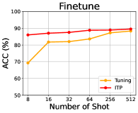
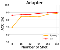
Figure 11: Performance variation of distillation-based recyclable tuning on IMDB at different data scales. We compare two methods: the conventional tuning method (Tuning), and our interpolation distillation method (ITP).

Taking a step further, we study the performance of our distillation-based recyclable tuning at different data scales. Specifically, we focus on $\mathcal{T}_{2}$ (IMDB) for recycling $\mathcal{M}_{1}$’s outdated weights to $\mathcal{M}_{2}$, where $\mathcal{M}_{1}$ is adapted using the full dataset, and $\mathcal{M}_{2}$ is trained with $\{8,16,32,64\}$-shot dataset, respectively. By comparing the method mentioned in § C.5 ($\mathcal{L}_{\text{ITP}}$) with only the task loss $\mathcal{L}_{\mathcal{T}}$, we visualize the performance variation in Figure 11, from which we observe that: $\mathcal{L}_{\text{ITP}}$ surpasses only the task loss ($\mathcal{L}_{\mathcal{T}}$) in general. However, with the data scale increasing, the improvement becomes smaller. This is because $\mathcal{M}_{2}$ is more adept at $\mathcal{T}_{2}$ than $\mathcal{M}_{1}$ due to the incremental knowledge acquisition of $\mathcal{D}_{2}$. When there are only a few examples to train $\mathcal{M}_{2}$, the teacher model has the advantage of more labeled data. However, with the data size of the student gradually approaching that of the teacher, learning from the teacher gradually becomes redundant. The student model could well master the downstream knowledge on its own.

Appendix D Training Details

We ensure that all the artifacts used in this paper are consistent with their intended use.

Task	LR	BS	S/E(AP)	S/E(FT)
ChemProt	$2\times 10^{-5}$	$16$	$25$ epochs	$10$ epochs
IMDB	$2\times 10^{-5}$	$16$	$25$ epochs	$10$ epochs
ACL-ARC	$2\times 10^{-5}$	$16$	$25$ epochs	$10$ epochs
MNLI	$2\times 10^{-5}$	$32$	$50$k steps	$50$k steps
ANLI	$2\times 10^{-5}$	$32$	$50$k steps	$50$k steps
SICK	$2\times 10^{-5}$	$32$	$50$k steps	$50$k steps
R. Tomatoes	$2\times 10^{-5}$	$32$	$50$k steps	$50$k steps
A. Polarity	$2\times 10^{-5}$	$16$	$15$k steps	$15$k steps
SST-2	$2\times 10^{-5}$	$16$	$15$k steps	$15$k steps
H. Speech	$2\times 10^{-5}$	$16$	$15$k steps	$15$k steps
T. Hate	$2\times 10^{-5}$	$16$	$15$k steps	$15$k steps
T. Offensive	$2\times 10^{-5}$	$16$	$15$k steps	$15$k steps

Table 11: Hyper-parameters used for downstream adaptation (LR: learning rate, BS: batch size, S / E: maximum step / maximum epoch. AP and FT refer to adapter tuning and fine-tuning.

D.1 Pre-training

We conduct pre-training using $8$ NVIDIA V100 GPUs based on fairseq Ott et al. (2019). We choose Adam (Kingma and Ba, 2015) as the optimizer. The hyper-parameters ($\epsilon,\beta_{1},\beta_{2}$) for Adam are set to $1\times 10^{-6},0.9,0.98$, respectively. The dropout rate and weight decay are set to $0.1$ and $0.01$, respectively. The total number of parameters of $\text{RoBERTa}_{\texttt{BASE}}$ and $\text{RoBERTa}_{\texttt{LARGE}}$ are $125$M and $355$M, respectively. We implement pre-training using the codes of Qin et al. (2022a).

Continual Pre-training.

We start with the official RoBERTa model and sequentially pre-train the PLM on $4$ domains. For each domain, we set the batch size to $2048$, the training steps to $12.5$k, and the max sequence length to $512$.

Pre-training from Scratch.

For $\mathcal{M}_{\text{IND}}$ that is pre-trained from scratch, we follow the model structure of $\text{RoBERTa}_{\texttt{BASE}}$, and pre-train the model on the concatenation of Wikipedia and BookCorpus (Zhu et al., 2015), which is the same as the pre-training corpus of BERT (Devlin et al., 2019). We pre-train the model for $125$k steps, using a batch size of $2048$ and a sequence length of $512$. The total computations involved are roughly comparable to those of $\text{BERT}_{\texttt{BASE}}$. $\mathcal{M}_{\text{IND}}$ has totally different initialization and pre-training corpus than the official $\text{RoBERTa}_{\texttt{BASE}}$, which helps us understand the property between independently trained PLMs.

D.2 Empirical Analyses

Model Compatibility Analysis.

We adapt the initial PLM $\mathcal{M}_{0}$ on two tasks ChemProt and MNLI. The training hyper-parameters conform to those listed in Table 11. All experiments are conducted $3$ times with different random seeds, and we report the average results.

Linear Mode Connectivity Analysis.

All the training hyper-parameters conform to those in Table 11. The endpoints are adapted three times using different random seeds. We test the performance of $25$ evenly distributed points along the linear path and two endpoints. We report the average performance over three random seeds.

Target Task	$\mathcal{T}_{\text{diff}}$	$\mathcal{T}_{\text{sim}}$	EI (steps)
ANLI	SST-2	MNLI	$1000$
SICK	SST-2	MNLI	$50$
SST-2	MNLI	A. Polarity	$60$
R. Tomatoes	MNLI	A. Polarity	$100$
H. Speech	MNLI	T. Hate	$300$
T. Offensive	MNLI	T. Hate	$40$

Table 12: The selection of source tasks and target tasks for experiments in § 5.1. For each target task, we list both $\mathcal{T}_{\text{diff}}$ and $\mathcal{T}_{\text{sim}}$. We also report the evaluation interval (EI) w.r.t. training steps for each of the $6$ target tasks.

Functional Similarity Analysis.

We adapt different PLMs on task ChemProt using the hyper-parameters listed in Table 11. We randomly sample one instance from ChemProt and feed it into different PLMs to obtain the scores after the self-attention computation. We draw the attention scores for the first $25$ tokens of the sampled instance.

D.3 Methods and Experiments

For the optimizer of all the experiments in § 5, we choose AdamW (Loshchilov and Hutter, 2019).

Initialization-based Recyclable Tuning.

We adapt $\mathcal{M}_{0}$ on the source tasks using the hyper-parameters listed in Table 11. The adapted weights are further used as target tasks’ initialization (except the Random setting). The target tasks’ training configurations also conform to Table 11. We conduct the experiments for $3$ times with different random seeds and report the average performance. The choices of $\mathcal{T}_{\text{diff}}$ and $\mathcal{T}_{\text{sim}}$ for different target tasks are shown in Table 12. The evaluation interval for each target task is also reported in Table 12.

Distillation-based Recyclable Tuning.

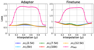
Figure 12: The loss of linear interpolations between two adapted PLMs ($\theta_{0}^{\mathcal{T}}$ and $\theta_{1}^{\mathcal{T}}(t)$) on ChemProt. The corresponding visualization for performance is shown in Figure 3.

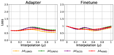
Figure 13: Mode connectivity (loss evaluation) between continually pre-trained PLMs across $4$ domains and the initial $\mathcal{M}_{0}$. The corresponding visualization for performance is shown in Figure 4.

We set the maximum training step for ChemProt and ACL-ARC to $100$k and the maximum training step for IMDB to $50$k. The learning rate and batch size are set to $1\times 10^{-4}$ and $2$, respectively. We warm up the learning rate for the first $8\%$ percentage of total training steps. We report the average results over $3$ different random seeds. As for other hyper-parameters discussed in § 5.2, we perform grid search for $\beta$ over {$0.1$, $0.3$}, and $\alpha(1-\beta)$ over {$0$, $1$, $5$, $10$, $50$, $100$}. We also conduct a grid search for the temperature in knowledge distillation loss over {$10$, $20$} when calculating $\textrm{KL}(\mathcal{P}(x,\mathcal{M}_{i})||\mathcal{P}(x,\mathcal{M}_{i+1}))$. We select the best-performing combination of these hyper-parameters and then report the performance. Our grid search is performed for our method and all the baseline methods for a fair comparison.

Appendix E The Visualization of Loss for Linear Mode Connectivity Analysis

When conducting experiments for the mode connectivity analysis in the main paper, we mainly resort to performance as the evaluation protocol for the interpolations following Qin et al. (2022b). In this section, we show the corresponding visualization of loss for Figure 3 and Figure 4, see Figure 12 and Figure 13. From these figures, we conclude that a significant loss barrier generally indicates the existence of a large performance drop.

Appendix F Comparison of Initialization-based and Distillation-based Recyclable Tuning

Both initialization-based and distillation-based methods serve as powerful ways for recyclable tuning under the continual pre-training scenario. Both methods have their own advantages, where the initialization-based method can bring faster convergence and performance improvement, while the distillation-based method can bring improvement in performance as well (but may be less efficient). In addition, both methods can be combined with each other to further improve performance.

In terms of practical application scenarios, both methods are slightly different. For one thing, the initialization-based method requires that the architectures of the new PLM and the old PLM are the same. This requirement may be infeasible for broader application scenarios, such as recyclable tuning between different PLMs as discussed in § 6. For another, the initialization-based method typically requires access to the parameters of the outdated adapted weights. This can be a practical issue due to model privacy concerns. While some customers are willing to share their adapted weights on public platforms like AdapterHub (Pfeiffer et al., 2020), a majority of adapted weights are publicly unavailable. In contrast, the distillation-based method can be achieved without access to the model weights, but through receiving model inference from the owner (e.g., API-based online knowledge transfer (Krishna et al., 2019)). In this sense, the distillation-based method could protect the model privacy to a certain degree.

Broader Impacts

This research has the potential to have a broad impact in several ways.

• First, recyclable tuning could improve the efficiency of adapting PLMs to new tasks. By recycling adapted weights from previous tasks, the need for costly retraining can be reduced, potentially making it more feasible to apply PLMs in a wider range of scenarios.

• Second, the results of this research could have implications for the sustainability of machine learning systems. Reusing adapted weights rather than discarding them can help us reduce the carbon footprint and resource consumption of PLM adaptation, making it more environmentally friendly.

• Third, this research has the potential to benefit a wide range of stakeholders, including researchers, developers, and users of PLMs. Researchers can use the proposed task and benchmark to develop and evaluate new techniques for recyclable tuning, while developers can apply these techniques to improve the efficiency and sustainability of PLM-based systems. Finally, users of PLMs can benefit from the reduced costs and improved performance made possible by recyclable tuning.

Overall, this research on recyclable tuning for continual pre-training has the potential to have a wide-ranging impact on the efficiency, sustainability, and practicality of machine learning systems.

References

- Aghajanyan et al. (2021) Armen Aghajanyan, Anchit Gupta, Akshat Shrivastava, Xilun Chen, Luke Zettlemoyer, and Sonal Gupta. 2021. Muppet: Massive multi-task representations with pre-finetuning. In Proceedings of the 2021 Conference on Empirical Methods in Natural Language Processing, pages 5799–5811, Online and Punta Cana, Dominican Republic. Association for Computational Linguistics.
- Barbieri et al. (2020) Francesco Barbieri, Jose Camacho-Collados, Luis Espinosa Anke, and Leonardo Neves. 2020. TweetEval: Unified benchmark and comparative evaluation for tweet classification. In Findings of the Association for Computational Linguistics: EMNLP 2020, pages 1644–1650, Online. Association for Computational Linguistics.
- Bommasani et al. (2021) Rishi Bommasani, Drew A Hudson, Ehsan Adeli, Russ Altman, Simran Arora, Sydney von Arx, Michael S Bernstein, Jeannette Bohg, Antoine Bosselut, Emma Brunskill, et al. 2021. On the opportunities and risks of foundation models. arXiv preprint arXiv:2108.07258.
- Brown et al. (2020) Tom B. Brown, Benjamin Mann, Nick Ryder, Melanie Subbiah, Jared Kaplan, Prafulla Dhariwal, Arvind Neelakantan, Pranav Shyam, Girish Sastry, Amanda Askell, Sandhini Agarwal, Ariel Herbert-Voss, Gretchen Krueger, Tom Henighan, Rewon Child, Aditya Ramesh, Daniel M. Ziegler, Jeffrey Wu, Clemens Winter, Christopher Hesse, Mark Chen, Eric Sigler, Mateusz Litwin, Scott Gray, Benjamin Chess, Jack Clark, Christopher Berner, Sam McCandlish, Alec Radford, Ilya Sutskever, and Dario Amodei. 2020. Language models are few-shot learners. In Advances in Neural Information Processing Systems 33: Annual Conference on Neural Information Processing Systems 2020, NeurIPS 2020, December 6-12, 2020, virtual.
- Chen et al. (2022) Cheng Chen, Yichun Yin, Lifeng Shang, Xin Jiang, Yujia Qin, Fengyu Wang, Zhi Wang, Xiao Chen, Zhiyuan Liu, and Qun Liu. 2022. bert2BERT: Towards reusable pretrained language models. In Proceedings of the 60th Annual Meeting of the Association for Computational Linguistics (Volume 1: Long Papers), pages 2134–2148, Dublin, Ireland. Association for Computational Linguistics.
- Davidson et al. (2017) Thomas Davidson, Dana Warmsley, Michael Macy, and Ingmar Weber. 2017. Automated hate speech detection and the problem of offensive language. In Proceedings of the 11th International AAAI Conference on Web and Social Media, ICWSM ’17, pages 512–515.
- Devlin et al. (2019) Jacob Devlin, Ming-Wei Chang, Kenton Lee, and Kristina Toutanova. 2019. BERT: Pre-training of deep bidirectional transformers for language understanding. In Proceedings of the 2019 Conference of the North American Chapter of the Association for Computational Linguistics: Human Language Technologies, Volume 1 (Long and Short Papers), pages 4171–4186, Minneapolis, Minnesota. Association for Computational Linguistics.
- Ding et al. (2022) Ning Ding, Yujia Qin, Guang Yang, Fuchao Wei, Zonghan Yang, Yusheng Su, Shengding Hu, Yulin Chen, Chi-Min Chan, Weize Chen, et al. 2022. Delta tuning: A comprehensive study of parameter efficient methods for pre-trained language models. arXiv preprint arXiv:2203.06904.
- Draxler et al. (2018) Felix Draxler, Kambis Veschgini, Manfred Salmhofer, and Fred A. Hamprecht. 2018. Essentially no barriers in neural network energy landscape. In Proceedings of the 35th International Conference on Machine Learning, ICML 2018, Stockholmsmässan, Stockholm, Sweden, July 10-15, 2018, volume 80 of Proceedings of Machine Learning Research, pages 1308–1317. PMLR.
- Faruqui and Das (2018) Manaal Faruqui and Dipanjan Das. 2018. Identifying well-formed natural language questions. In Proceedings of the 2018 Conference on Empirical Methods in Natural Language Processing, pages 798–803, Brussels, Belgium. Association for Computational Linguistics.
- Frankle et al. (2020) Jonathan Frankle, Gintare Karolina Dziugaite, Daniel Roy, and Michael Carbin. 2020. Linear mode connectivity and the lottery ticket hypothesis. In Proceedings of the 37th International Conference on Machine Learning, ICML 2020, 13-18 July 2020, Virtual Event, volume 119 of Proceedings of Machine Learning Research, pages 3259–3269. PMLR.
- Freeman and Bruna (2017) C. Daniel Freeman and Joan Bruna. 2017. Topology and geometry of half-rectified network optimization. In 5th International Conference on Learning Representations, ICLR 2017, Toulon, France, April 24-26, 2017, Conference Track Proceedings. OpenReview.net.
- Garipov et al. (2018) Timur Garipov, Pavel Izmailov, Dmitrii Podoprikhin, Dmitry P. Vetrov, and Andrew Gordon Wilson. 2018. Loss surfaces, mode connectivity, and fast ensembling of dnns. In Advances in Neural Information Processing Systems 31: Annual Conference on Neural Information Processing Systems 2018, NeurIPS 2018, December 3-8, 2018, Montréal, Canada, pages 8803–8812.
- Gong et al. (2019) Linyuan Gong, Di He, Zhuohan Li, Tao Qin, Liwei Wang, and Tieyan Liu. 2019. Efficient training of BERT by progressively stacking. In Proceedings of the 36th International Conference on Machine Learning, volume 97 of Proceedings of Machine Learning Research, pages 2337–2346. PMLR.
- Gururangan et al. (2020) Suchin Gururangan, Ana Marasović, Swabha Swayamdipta, Kyle Lo, Iz Beltagy, Doug Downey, and Noah A. Smith. 2020. Don’t stop pretraining: Adapt language models to domains and tasks. In Proceedings of the 58th Annual Meeting of the Association for Computational Linguistics, pages 8342–8360, Online. Association for Computational Linguistics.
- He and McAuley (2016) Ruining He and Julian J. McAuley. 2016. Ups and downs: Modeling the visual evolution of fashion trends with one-class collaborative filtering. In Proceedings of the 25th International Conference on World Wide Web, WWW 2016, Montreal, Canada, April 11 - 15, 2016, pages 507–517. ACM.
- Hinton et al. (2015) Geoffrey Hinton, Oriol Vinyals, and Jeff Dean. 2015. Distilling the knowledge in a neural network. ArXiv preprint, abs/1503.02531.
- Houlsby et al. (2019) Neil Houlsby, Andrei Giurgiu, Stanislaw Jastrzebski, Bruna Morrone, Quentin De Laroussilhe, Andrea Gesmundo, Mona Attariyan, and Sylvain Gelly. 2019. Parameter-efficient transfer learning for NLP. In Proceedings of the 36th International Conference on Machine Learning, volume 97 of Proceedings of Machine Learning Research, pages 2790–2799. PMLR.
- Jang et al. (2022) Joel Jang, Seonghyeon Ye, Changho Lee, Sohee Yang, Joongbo Shin, Janghoon Han, Gyeonghun Kim, and Minjoon Seo. 2022. Temporalwiki: A lifelong benchmark for training and evaluating ever-evolving language models.
- Jang et al. (2021) Joel Jang, Seonghyeon Ye, Sohee Yang, Joongbo Shin, Janghoon Han, Gyeonghun Kim, Stanley Jungkyu Choi, and Minjoon Seo. 2021. Towards continual knowledge learning of language models. ArXiv preprint, abs/2110.03215.
- Jin et al. (2022) Xisen Jin, Dejiao Zhang, Henghui Zhu, Wei Xiao, Shang-Wen Li, Xiaokai Wei, Andrew Arnold, and Xiang Ren. 2022. Lifelong pretraining: Continually adapting language models to emerging corpora. In Proceedings of BigScience Episode #5 – Workshop on Challenges & Perspectives in Creating Large Language Models, pages 1–16, virtual+Dublin. Association for Computational Linguistics.
- Jurgens et al. (2018) David Jurgens, Srijan Kumar, Raine Hoover, Dan McFarland, and Dan Jurafsky. 2018. Measuring the evolution of a scientific field through citation frames. Transactions of the Association for Computational Linguistics, 6:391–406.
- Khashabi et al. (2020) Daniel Khashabi, Sewon Min, Tushar Khot, Ashish Sabharwal, Oyvind Tafjord, Peter Clark, and Hannaneh Hajishirzi. 2020. UNIFIEDQA: Crossing format boundaries with a single QA system. In Findings of the Association for Computational Linguistics: EMNLP 2020, pages 1896–1907, Online. Association for Computational Linguistics.
- Kingma and Ba (2015) Diederik P. Kingma and Jimmy Ba. 2015. Adam: A method for stochastic optimization. In 3rd International Conference on Learning Representations, ICLR 2015, San Diego, CA, USA, May 7-9, 2015, Conference Track Proceedings.
- Kringelum et al. (2016) Jens Kringelum, Sonny Kim Kjaerulff, Søren Brunak, Ole Lund, Tudor I Oprea, and Olivier Taboureau. 2016. Chemprot-3.0: a global chemical biology diseases mapping. Database, 2016.
- Krishna et al. (2019) Kalpesh Krishna, Gaurav Singh Tomar, Ankur P Parikh, Nicolas Papernot, and Mohit Iyyer. 2019. Thieves on sesame street! model extraction of bert-based apis. arXiv preprint arXiv:1910.12366.
- Lee-Thorp et al. (2022) James Lee-Thorp, Joshua Ainslie, Ilya Eckstein, and Santiago Ontanon. 2022. FNet: Mixing tokens with Fourier transforms. In Proceedings of the 2022 Conference of the North American Chapter of the Association for Computational Linguistics: Human Language Technologies, pages 4296–4313, Seattle, United States. Association for Computational Linguistics.
- Lin et al. (2021) Ye Lin, Yanyang Li, Ziyang Wang, Bei Li, Quan Du, Tong Xiao, and Jingbo Zhu. 2021. Weight distillation: Transferring the knowledge in neural network parameters. In Proceedings of the 59th Annual Meeting of the Association for Computational Linguistics and the 11th International Joint Conference on Natural Language Processing (Volume 1: Long Papers), pages 2076–2088, Online. Association for Computational Linguistics.
- Liu et al. (2019) Yinhan Liu, Myle Ott, Naman Goyal, Jingfei Du, Mandar Joshi, Danqi Chen, Omer Levy, Mike Lewis, Luke Zettlemoyer, and Veselin Stoyanov. 2019. RoBERTa: A robustly optimized BERT pretraining approach. ArXiv preprint, abs/1907.11692.
- Lo et al. (2020) Kyle Lo, Lucy Lu Wang, Mark Neumann, Rodney Kinney, and Daniel Weld. 2020. S2ORC: The semantic scholar open research corpus. In Proceedings of the 58th Annual Meeting of the Association for Computational Linguistics, pages 4969–4983, Online. Association for Computational Linguistics.
- Loshchilov and Hutter (2019) Ilya Loshchilov and Frank Hutter. 2019. Decoupled weight decay regularization. In 7th International Conference on Learning Representations, ICLR 2019, New Orleans, LA, USA, May 6-9, 2019. OpenReview.net.
- Maas et al. (2011) Andrew L. Maas, Raymond E. Daly, Peter T. Pham, Dan Huang, Andrew Y. Ng, and Christopher Potts. 2011. Learning word vectors for sentiment analysis. In Proceedings of the 49th Annual Meeting of the Association for Computational Linguistics: Human Language Technologies, pages 142–150, Portland, Oregon, USA. Association for Computational Linguistics.
- Marelli et al. (2014) Marco Marelli, Stefano Menini, Marco Baroni, Luisa Bentivogli, Raffaella Bernardi, and Roberto Zamparelli. 2014. A sick cure for the evaluation of compositional distributional semantic models. In Proceedings of the Ninth International Conference on Language Resources and Evaluation (LREC’14), pages 216–223.
- McAuley and Leskovec (2013) Julian McAuley and Jure Leskovec. 2013. Hidden factors and hidden topics: understanding rating dimensions with review text. In Proceedings of the 7th ACM conference on Recommender systems, pages 165–172.
- Mirzadeh et al. (2020) Seyed Iman Mirzadeh, Mehrdad Farajtabar, Dilan Gorur, Razvan Pascanu, and Hassan Ghasemzadeh. 2020. Linear mode connectivity in multitask and continual learning. arXiv preprint arXiv:2010.04495.
- Nie et al. (2020) Yixin Nie, Adina Williams, Emily Dinan, Mohit Bansal, Jason Weston, and Douwe Kiela. 2020. Adversarial NLI: A new benchmark for natural language understanding. In Proceedings of the 58th Annual Meeting of the Association for Computational Linguistics, pages 4885–4901, Online. Association for Computational Linguistics.
- Ott et al. (2019) Myle Ott, Sergey Edunov, Alexei Baevski, Angela Fan, Sam Gross, Nathan Ng, David Grangier, and Michael Auli. 2019. fairseq: A fast, extensible toolkit for sequence modeling. In Proceedings of the 2019 Conference of the North American Chapter of the Association for Computational Linguistics (Demonstrations), pages 48–53, Minneapolis, Minnesota. Association for Computational Linguistics.
- Pang and Lee (2005) Bo Pang and Lillian Lee. 2005. Seeing stars: Exploiting class relationships for sentiment categorization with respect to rating scales. In Proceedings of the 43rd Annual Meeting of the Association for Computational Linguistics (ACL’05), pages 115–124, Ann Arbor, Michigan. Association for Computational Linguistics.
- Paszke et al. (2019) Adam Paszke, Sam Gross, Francisco Massa, Adam Lerer, James Bradbury, Gregory Chanan, Trevor Killeen, Zeming Lin, Natalia Gimelshein, Luca Antiga, et al. 2019. Pytorch: An imperative style, high-performance deep learning library. Advances in neural information processing systems, 32.
- Pfeiffer et al. (2020) Jonas Pfeiffer, Andreas Rücklé, Clifton Poth, Aishwarya Kamath, Ivan Vulić, Sebastian Ruder, Kyunghyun Cho, and Iryna Gurevych. 2020. Adapterhub: A framework for adapting transformers. In Proceedings of the 2020 Conference on Empirical Methods in Natural Language Processing: System Demonstrations, pages 46–54.
- Poth et al. (2021) Clifton Poth, Jonas Pfeiffer, Andreas Rücklé, and Iryna Gurevych. 2021. What to pre-train on? Efficient intermediate task selection. In Proceedings of the 2021 Conference on Empirical Methods in Natural Language Processing, pages 10585–10605, Online and Punta Cana, Dominican Republic. Association for Computational Linguistics.
- Qin et al. (2022a) Yujia Qin, Yankai Lin, Jing Yi, Jiajie Zhang, Xu Han, Zhengyan Zhang, Yusheng Su, Zhiyuan Liu, Peng Li, Maosong Sun, and Jie Zhou. 2022a. Knowledge inheritance for pre-trained language models. In Proceedings of the 2022 Conference of the North American Chapter of the Association for Computational Linguistics: Human Language Technologies, pages 3921–3937, Seattle, United States. Association for Computational Linguistics.
- Qin et al. (2022b) Yujia Qin, Cheng Qian, Jing Yi, Weize Chen, Yankai Lin, Xu Han, Zhiyuan Liu, Maosong Sun, and Jie Zhou. 2022b. Exploring mode connectivity for pre-trained language models. arXiv preprint arXiv:2210.14102.
- Qin et al. (2021) Yujia Qin, Xiaozhi Wang, Yusheng Su, Yankai Lin, Ning Ding, Zhiyuan Liu, Juanzi Li, Lei Hou, Peng Li, Maosong Sun, et al. 2021. Exploring low-dimensional intrinsic task subspace via prompt tuning. arXiv preprint arXiv:2110.07867.
- Qin et al. (2022c) Yujia Qin, Jiajie Zhang, Yankai Lin, Zhiyuan Liu, Peng Li, Maosong Sun, and Jie Zhou. 2022c. ELLE: Efficient lifelong pre-training for emerging data. In Findings of the Association for Computational Linguistics: ACL 2022, pages 2789–2810, Dublin, Ireland. Association for Computational Linguistics.
- Raffel et al. (2020) Colin Raffel, Noam Shazeer, Adam Roberts, Katherine Lee, Sharan Narang, Michael Matena, Yanqi Zhou, Wei Li, and Peter J. Liu. 2020. Exploring the limits of transfer learning with a unified text-to-text transformer. Journal of Machine Learning Research, 21(140):1–67.
- Rajpurkar et al. (2016) Pranav Rajpurkar, Jian Zhang, Konstantin Lopyrev, and Percy Liang. 2016. SQuAD: 100,000+ questions for machine comprehension of text. In Proceedings of the 2016 Conference on Empirical Methods in Natural Language Processing, pages 2383–2392, Austin, Texas. Association for Computational Linguistics.
- Sanh et al. (2021) Victor Sanh, Albert Webson, Colin Raffel, Stephen H Bach, Lintang Sutawika, Zaid Alyafeai, Antoine Chaffin, Arnaud Stiegler, Teven Le Scao, Arun Raja, et al. 2021. Multitask prompted training enables zero-shot task generalization. arXiv preprint arXiv:2110.08207.
- Schick and Schütze (2021) Timo Schick and Hinrich Schütze. 2021. Exploiting cloze-questions for few-shot text classification and natural language inference. In Proceedings of the 16th Conference of the European Chapter of the Association for Computational Linguistics: Main Volume, pages 255–269, Online. Association for Computational Linguistics.
- Socher et al. (2013) Richard Socher, Alex Perelygin, Jean Wu, Jason Chuang, Christopher D. Manning, Andrew Ng, and Christopher Potts. 2013. Recursive deep models for semantic compositionality over a sentiment treebank. In Proceedings of the 2013 Conference on Empirical Methods in Natural Language Processing, pages 1631–1642, Seattle, Washington, USA. Association for Computational Linguistics.
- Su et al. (2022) Yusheng Su, Xiaozhi Wang, Yujia Qin, Chi-Min Chan, Yankai Lin, Huadong Wang, Kaiyue Wen, Zhiyuan Liu, Peng Li, Juanzi Li, Lei Hou, Maosong Sun, and Jie Zhou. 2022. On transferability of prompt tuning for natural language processing. In Proceedings of the 2022 Conference of the North American Chapter of the Association for Computational Linguistics: Human Language Technologies, pages 3949–3969, Seattle, United States. Association for Computational Linguistics.
- Sun et al. (2019) Siqi Sun, Yu Cheng, Zhe Gan, and Jingjing Liu. 2019. Patient knowledge distillation for BERT model compression. In Proceedings of the 2019 Conference on Empirical Methods in Natural Language Processing and the 9th International Joint Conference on Natural Language Processing (EMNLP-IJCNLP), pages 4323–4332, Hong Kong, China. Association for Computational Linguistics.
- Vaswani et al. (2017) Ashish Vaswani, Noam Shazeer, Niki Parmar, Jakob Uszkoreit, Llion Jones, Aidan N. Gomez, Lukasz Kaiser, and Illia Polosukhin. 2017. Attention is all you need. In Advances in Neural Information Processing Systems 30: Annual Conference on Neural Information Processing Systems 2017, December 4-9, 2017, Long Beach, CA, USA, pages 5998–6008.
- Vu et al. (2020) Tu Vu, Tong Wang, Tsendsuren Munkhdalai, Alessandro Sordoni, Adam Trischler, Andrew Mattarella-Micke, Subhransu Maji, and Mohit Iyyer. 2020. Exploring and predicting transferability across NLP tasks. In Proceedings of the 2020 Conference on Empirical Methods in Natural Language Processing (EMNLP), pages 7882–7926, Online. Association for Computational Linguistics.
- Williams et al. (2018) Adina Williams, Nikita Nangia, and Samuel Bowman. 2018. A broad-coverage challenge corpus for sentence understanding through inference. In Proceedings of the 2018 Conference of the North American Chapter of the Association for Computational Linguistics: Human Language Technologies, Volume 1 (Long Papers), pages 1112–1122, New Orleans, Louisiana. Association for Computational Linguistics.
- Wolf et al. (2020) Thomas Wolf, Lysandre Debut, Victor Sanh, Julien Chaumond, Clement Delangue, Anthony Moi, Pierric Cistac, Tim Rault, Rémi Louf, Morgan Funtowicz, Joe Davison, Sam Shleifer, Patrick von Platen, Clara Ma, Yacine Jernite, Julien Plu, Canwen Xu, Teven Le Scao, Sylvain Gugger, Mariama Drame, Quentin Lhoest, and Alexander M. Rush. 2020. Transformers: State-of-the-art natural language processing. In Proceedings of the 2020 Conference on Empirical Methods in Natural Language Processing: System Demonstrations, pages 38–45, Online. Association for Computational Linguistics.
- Wu et al. (2021) Tongtong Wu, Massimo Caccia, Zhuang Li, Yuan-Fang Li, Guilin Qi, and Gholamreza Haffari. 2021. Pretrained language model in continual learning: A comparative study. In International Conference on Learning Representations.
- Yi et al. (2022) Jing Yi, Weize Chen, Yujia Qin, Yankai Lin, Ning Ding, Xu Han, Zhiyuan Liu, Maosong Sun, and Jie Zhou. 2022. Different tunes played with equal skill: Exploring a unified optimization subspace for parameter-efficient tuning. In Findings of the Association for Computational Linguistics: EMNLP 2022, pages 3348–3366, Abu Dhabi, United Arab Emirates. Association for Computational Linguistics.
- Zellers et al. (2019) Rowan Zellers, Ari Holtzman, Hannah Rashkin, Yonatan Bisk, Ali Farhadi, Franziska Roesner, and Yejin Choi. 2019. Defending against neural fake news. In Advances in Neural Information Processing Systems 32: Annual Conference on Neural Information Processing Systems 2019, NeurIPS 2019, December 8-14, 2019, Vancouver, BC, Canada, pages 9051–9062.
- Zhu et al. (2015) Yukun Zhu, Ryan Kiros, Richard S. Zemel, Ruslan Salakhutdinov, Raquel Urtasun, Antonio Torralba, and Sanja Fidler. 2015. Aligning books and movies: Towards story-like visual explanations by watching movies and reading books. In 2015 IEEE International Conference on Computer Vision, ICCV 2015, Santiago, Chile, December 7-13, 2015, pages 19–27. IEEE Computer Society.