Mixed finite elements for Kirchhoff–Love plate bending

Abstract

We present a mixed finite element method with triangular and parallelogram meshes for the Kirchhoff–Love plate bending model. Critical ingredient is the construction of low-dimensional local spaces and appropriate degrees of freedom that provide conformity in terms of a sufficiently large tensor space and that allow for any kind of physically relevant Dirichlet and Neumann boundary conditions. For Dirichlet boundary conditions and polygonal plates, we prove quasi-optimal convergence of the mixed scheme. An a posteriori error estimator is derived for the special case of the biharmonic problem. Numerical results for regular and singular examples illustrate our findings. They confirm expected convergence rates and exemplify the performance of an adaptive algorithm steered by our error estimator.

AMS Subject Classification: 74S05, 35J35, 65N30, 74K20

1 Introduction

Plate bending models have been the subject of research in numerical analysis for several decades, until today. This is not only due to their relevance in structural engineering but also owed to the inherent mathematical challenges. The Kirchhoff–Love and Reissner–Mindlin models are the classical ones. The former can be interpreted as the singularly perturbed limit of the latter for plate thickness tending to zero. This limit case poses the vertical deflection $u$ as an $H^{2}(\Omega)$-function whereas the bending moments $\boldsymbol{M}$ are set in the space of symmetric $L_{2}(\Omega)$-tensors with $\operatorname{div}\operatorname{\mathbf{div}}\boldsymbol{M}\in L_{2}(\Omega)$ for $L_{2}$-regular vertical loads $f$, in short, $\boldsymbol{M}\in\mathbb{H}(\operatorname{div\mathbf{div}};\Omega)$. (Here, $\Omega\subset\mathbb{R}^{2}$ denotes the plate’s mid-surface, and $\operatorname{\mathbf{div}}\boldsymbol{M}$ means the row-wise application of the divergence operator.) For non-convex polygonal plates, $\mathbb{H}(\operatorname{div\mathbf{div}};\Omega)$ is not a subspace of ${\boldsymbol{H}}^{1}(\Omega)$ (tensors with $H^{1}(\Omega)$-components) or $\mathbb{H}(\operatorname{\mathbf{div}};\Omega)$ (symmetric tensors $\boldsymbol{M}$ with $\operatorname{\mathbf{div}}\boldsymbol{M}\in\boldsymbol{L}_{2}(\Omega):=L_{2}(\Omega)^{2}$), cf. [1]. This lack of regularity constitutes a serious challenge for the approximation of bending moments and its analysis. Bending moments are critical quantities in engineering applications and have been elusive to conforming approximations in $\mathbb{H}(\operatorname{div\mathbf{div}};\Omega)$ for a long time. An early, only partially conforming approach is the Hellan–Herrmann–Johnson method that gives bending moment approximations with continuous normal-normal traces, see [15, 16, 18].

In this paper, we present low-dimensional local spaces of lowest degree on triangles and parallelograms with corresponding basis functions. Their degrees of freedom provide $\mathbb{H}(\operatorname{div\mathbf{div}};\Omega)$-conformity without requiring any additional non-physical regularity, contrary to previous approaches for triangles, see [5, 17]. In contrast, [6] provides approximations requiring low regularity, though they are not explicit and use more degrees of freedom. More specifically, for triangles $K$, we introduce

$$\mathbb{X}(K)=\operatorname{\mathbf{sCurl}}(\boldsymbol{RT}^{2}(K))\oplus\boldsymbol{x}\boldsymbol{x}^{\top}P^{1}(K)=\operatorname{sym}(\boldsymbol{RT}^{0}(K)\otimes\boldsymbol{RT}^{1}(K)).$$

Here, $P^{p}(K)$ are polynomials of degree $\leq p$, $\boldsymbol{RT}^{p}(K)=\boldsymbol{P}^{p}(K)+\boldsymbol{x}P^{p}(K)$ is the Raviart–Thomas space of order $p$ and $\operatorname{\mathbf{sCurl}}(\cdot)=\tfrac{1}{2}(\operatorname{\mathbf{Curl}}(\cdot)+\operatorname{\mathbf{Curl}}(\cdot)^{\top})$. The dimension of this space is $15$. (Our space for parallelograms is analogously constructed and has 20 degrees of freedom.) In [6, Section 2.3] and references therein, space $\mathbb{Y}(K)=\mathbb{P}_{\mathrm{sym}}^{k}(K)$ with degree $k\geq 3$ is proposed, giving dimension $30$ for the lowest-order case $k=3$. An analogy for the difference between $\mathbb{X}(K)$ and $\mathbb{Y}(K)$ is the difference between Raviart–Thomas and Brezzi–Douglas–Marini elements for discretizations of $\boldsymbol{H}(\operatorname{div};\Omega)$-vector fields. Both spaces $\mathbb{X}(K)$ and $\mathbb{Y}(K)$ have approximation order two in $\mathbb{H}(\operatorname{div\mathbf{div}};K)$. In [6, Section 2.4], a reduced lowest-order element with $20$ degrees of freedom is presented. However, its implementation requires a basis that is dual to the degrees of freedom which can be a challenging task, cf. [6, p.14]. For this reason the authors propose a hybridized mixed method.

We mention that there are some classical mixed schemes for Kirchhoff–Love plates, see, e.g., [9, 3, 19]. They are based on the interpretation of the Kirchhoff–Love model (with isotropic homogeneous material) as the bi-Laplacian, $\Delta^{2}u=f$, and introducing $v=\Delta u$ as an independent variable, as proposed by Ciarlet and Raviart in [7]. This strategy requires more regularity than generally available ($v\in H^{1}(\Omega)$) and does not allow for general Neumann boundary conditions as $v$ is a non-physical variable. We remark that in [10], we presented a DPG-setting for the two-variable setting with $v=\Delta u$ that is well posed for non-convex domains and $L_{2}(\Omega)$-loads.

Our analysis employs techniques and tools that we have learned from our studies [12, 11] of the discontinuous Petrov–Galerkin (DPG) method in the context of plate bending. Whereas the DPG framework may seem to be very specialized and irrelevant for the analysis of classical Galerkin approaches including mixed schemes, we here illustrate that this view is not correct. The most common DPG setting is based on ultraweak formulations. Their analysis requires a specific formulation of trace operators and the discretization of their images, the resulting trace spaces. On the domain level, these traces give rise to precise conditions of conformity, e.g., across interfaces. For canonical spaces this is well known. For example, $H^{1}(\Omega)$-conformity requires continuity in the sense of $H^{1/2}$-traces and $\boldsymbol{H}(\operatorname{div};\Omega)$-conformity means the $H^{-1/2}$-continuity of normal components. There are spaces where such an approach to conformity is much more intricate, for instance $\mathbb{H}(\operatorname{div\mathbf{div}};\Omega)$ introduced before. We stress the fact that there is a key difference between the conformity in the full space and the conformity of piecewise polynomial (or otherwise) approximations. In the latter case, trace operators have to be localized. Considering that trace spaces are typically of fractional order, this is a serious challenge. To circumvent this problem one usually requires more regularity. For instance, normal traces of $\boldsymbol{H}(\operatorname{div};\Omega)$ are considered in $L_{2}$ rather than $H^{-1/2}$. The key point is to increase the regularity as little as possible in order not to exclude relevant cases of low regularity. In this paper, we present and analyze a conforming piecewise polynomial approximation of bending moments $\boldsymbol{M}$ which only requires a slightly increased regularity $\boldsymbol{M}\in\mathbb{H}(\operatorname{div\mathbf{div}};\Omega,\mathcal{E})$. Here, $\mathbb{H}(\operatorname{div\mathbf{div}};\Omega,\mathcal{E})\subset\mathbb{H}(\operatorname{div\mathbf{div}};\Omega)$ is a dense subspace (introduced in §2) and therefore, our construction is applicable without any additional regularity requirement.

We use the trace formulation from [12] to construct $\mathbb{H}(\operatorname{div\mathbf{div}};\Omega)$-conforming elements. In contrast to our DPG-setting, where we use lowest-order moments for both the normal-normal traces and the effective shear forces (plus vertex jumps of tangential-normal traces), here we additionally use their first-order moments. In this way, second-order approximations are achieved, in contrast to order one in [12] (though, second order can be easily achieved also in the DPG setting). There is an inherent piecewise polynomial $\mathbb{H}(\operatorname{div\mathbf{div}};\Omega)$-interpolation operator. It commutes with the $L_{2}$-projection onto piecewise linear polynomials. Therefore, we have the canonical ingredients to set up a mixed finite element scheme and prove second order convergence for sufficiently regular solutions. The vertical deflection is approximated in $L_{2}(\Omega)$ by piecewise linear polynomials and the bending moments are approximated in $\mathbb{H}(\operatorname{div\mathbf{div}};\Omega)$ by our basis functions.

We also derive an a posteriori error estimator for our mixed scheme. For simplicity we consider constant material properties which is equivalent to studying the biharmonic problem. An extension to piecewise constant coefficients is possible but not pursued here. Error estimators are critical for steering adaptive algorithms in order to resolve singularities. In the analysis we follow ideas and techniques from Carstensen [4] for Poisson-type problems. The main ingredient for proving reliability of the estimator is a Helmholtz decomposition for vector fields. Here, we consider a Helmholtz-type decomposition of symmetric tensors fields. It uses an $\operatorname{\mathbf{sCurl}}(\cdot)$-representation of tensors which are in the kernel of the $\operatorname{div\mathbf{div}}$ operator, see, e.g., [21] and references therein. We stress the fact that our error estimator is not restricted to using space $\mathbb{X}(K)$ but can be derived for other conforming discretizations as mentioned before.

An overview of the remainder is as follows. In Section 2 we introduce Sobolev spaces and norms, recall plate-specific trace operators and their properties, and discuss polynomial spaces and transformation tools. Fundamental to this paper is our conformity characterization by Proposition 1. Local and global finite element spaces are the subject of Section 3. Outcome is a piecewise polynomial interpolation operator that provides $\mathbb{H}(\operatorname{div\mathbf{div}};\Omega)$-conforming, second-order approximations (Proposition 8). The mixed formulation and finite element scheme for the Kirchhoff–Love plate being model are presented in Section 4. Theorem 10 establishes the quasi-optimal convergence of the scheme. Theoretical results in Section 4 are proved for Dirichlet boundary conditions. Though, we stress the fact that our setting allows for implementing Neumann and mixed boundary conditions as well. Corresponding proofs require more technical details and are left open here. In Section 5 we present an a posteriori error estimator for the bending moments, the Hessian of the deflection in the biharmonic case, and prove its reliability and local efficiency. Finally, in Section 6 we report on numerical experiments. They include the case of a non-convex domain and singular solution, and underline the performance of an adaptive scheme that is based on our error estimator. In Appendix A, we illustrate the construction of basis (shape) functions for triangles and parallelograms. This is useful for implementation.

2 Preparations

2.1 Sobolev spaces and trace operators

For a Lipschitz domain $\omega\subset\mathbb{R}^{2}$ we denote by $L_{p}(\omega)$ ($p\in[1,\infty]$) resp. $H^{s}(\omega)$ ($s\in[0,2]$) Lebesgue resp. Sobolev spaces. The Sobolev spaces are defined by real interpolation between $L_{2}(\omega)$ and $H^{2}(\omega)$. The canonical norm and inner product in $L_{2}(\omega)$ are denoted by $\|\cdot\|_{\omega}$ and $(\cdot\hskip 1.42262pt,\cdot)_{\omega}$. For spaces of vector-valued resp. tensor-valued functions we use boldfaced resp. blackboard boldfaced letters, e.g., $\boldsymbol{L}_{2}(\omega)=L_{2}(\omega;\mathbb{R}^{2})$ and $\mathbb{L}_{2}(\omega)=L_{2}(\omega;\mathbb{R}^{2\times 2})$. For spaces of symmetric tensor-valued functions we use $\mathbb{L}_{2,\mathrm{sym}}(\omega)$. For a boundary part $\gamma\subseteq\partial\omega$ we use $\langle\cdot\hskip 1.42262pt,\cdot\rangle_{\gamma}$ to denote either a duality or the $L_{2}(\gamma)$ inner product.

We follow [12] and introduce

$$\mathbb{H}(\operatorname{div\mathbf{div}};\omega):=\big{\{}\boldsymbol{M}\in\mathbb{L}_{2,\mathrm{sym}}(\omega)\,:\,\operatorname{div\mathbf{div}}\boldsymbol{M}\in L_{2}(\omega)\big{\}},$$

a Hilbert space with (squared) norm

$$\|\boldsymbol{M}\|_{\mathbb{H}(\operatorname{div\mathbf{div}};\omega)}^{2}=\|\boldsymbol{M}\|_{\omega}^{2}+\|\operatorname{div\mathbf{div}}\boldsymbol{M}\|_{\omega}^{2}.$$

Here, $\operatorname{\mathbf{div}}$ is the divergence operator applied row-wise. We also need $\operatorname{\mathbf{Curl}}{\boldsymbol{q}}$ which is the $\operatorname{curl}$ operator applied to each component of ${\boldsymbol{q}}$, and

$$\operatorname{\mathbf{sCurl}}{\boldsymbol{q}}=\frac{1}{2}\big{(}\operatorname{\mathbf{Curl}}{\boldsymbol{q}}+(\operatorname{\mathbf{Curl}}{\boldsymbol{q}})^{\top}\big{)}$$

is the symmetrized $\operatorname{curl}$ operator. In addition, $\operatorname{\mathbf{rot}}$ is the row-wise $\operatorname{rot}$ operator. Sobolev space $H^{2}(\omega)$ is equipped with the (squared) norm

$$\|z\|_{H^{2}(\omega)}^{2}=\|z\|_{\omega}^{2}+\|\boldsymbol{\nabla}\nabla z\|_{\omega}^{2}.$$

We introduce trace operators $\operatorname{tr}_{\omega}^{\mathrm{dDiv}}\colon\mathbb{H}(\operatorname{div\mathbf{div}};\omega)\to H^{2}(\omega)^{\prime}$ and $\operatorname{tr}_{\omega}^{\mathrm{Ggrad}}\colon H^{2}(\omega)\to\mathbb{H}(\operatorname{div\mathbf{div}};\omega)^{\prime}$ by

$$\operatorname{tr}_{\omega}^{\mathrm{dDiv}}(\boldsymbol{M})(z) :=\langle\operatorname{tr}_{\omega}^{\mathrm{dDiv}}\boldsymbol{M}\hskip 1.42262pt,z\rangle_{\partial\omega}:=(\operatorname{div\mathbf{div}}\boldsymbol{M}\hskip 1.42262pt,z)_{\omega}-(\boldsymbol{M}\hskip 1.42262pt,\boldsymbol{\nabla}\nabla z)_{\omega},$$ (1a)

$$\operatorname{tr}_{\omega}^{\mathrm{Ggrad}}(z)(\boldsymbol{M}) :=\langle\operatorname{tr}_{\omega}^{\mathrm{Ggrad}}z\hskip 1.42262pt,\boldsymbol{M}\rangle_{\partial\omega}:=\langle\operatorname{tr}_{\omega}^{\mathrm{dDiv}}\boldsymbol{M}\hskip 1.42262pt,z\rangle_{\partial\omega}$$ (1b)

for all $$\boldsymbol{M}\in\mathbb{H}(\operatorname{div\mathbf{div}};\omega) z\in H^{2}(\omega)$$, .

While these operators are defined via volume integrals it can be easily seen with integration by parts that they reduce to boundary terms for sufficiently smooth arguments.

For a Lipschitz domain $\Omega$ let $\mathcal{T}$ denote a regular decomposition into open triangles and parallelograms $K$ such that

$$\overline{\Omega}=\bigcup_{K\in\mathcal{T}}\overline{K}.$$

Here, by regular we mean that all elements are non-degenerate and two distinct but touching elements either share one vertex or one edge. In particular, there are no hanging nodes. The set of edges of the mesh is denoted by $\mathcal{E}$ and the set of vertices by $\mathcal{V}$. We use $\mathcal{E}_{K}$, $\mathcal{V}_{K}$ to denote the edges, vertices of an element $K\in\mathcal{T}$. Furthermore, $\mathcal{V}_{\Omega}$ means the set of all interior vertices and $\mathcal{V}_{\Gamma}$ are the boundary vertices. The analogous notation is used for edges. The set $\omega_{\mathcal{T}}(z)=\big{\{}K\in\mathcal{T}\,:\,z\in\mathcal{V}_{K}\big{\}}$ is the neighborhood of vertex $z$ with corresponding domain $\Omega_{\mathcal{T}}(z)$. For elements $K\in\mathcal{T}$ we use the notation $\omega_{\mathcal{T}}(K)=\bigcup_{z\in\mathcal{V}_{K}}\omega_{\mathcal{T}}(z)$ and $\Omega_{\mathcal{T}}(K)$ for the corresponding domain. The triangular reference element $\widehat{K}_{\triangle}$ is the interior of the convex hull of vertices $(0,0)$, $(1,0)$, and $(0,1)$, and the square reference element $\widehat{K}_{\square}$ is the interior of the convex hull of vertices $(0,0)$, $(1,0)$, $(1,1)$, and $(0,1)$. In what follows we use the symbol $\widehat{K}$ to denote either $\widehat{K}_{\triangle}$ or $\widehat{K}_{\square}$. The diameter of an element $K$ resp. edge $E$ is denoted by $h_{K}$ resp. $h_{E}$. We define the mesh-size function $h_{\mathcal{T}}\in L_{\infty}(\Omega)$ by $h_{\mathcal{T}}|_{K}=h_{K}$. Moreover, we assume that $\mathcal{T}$ is a decomposition of $\Omega$ into shape-regular elements. This implies that neighboring elements have comparable diameters as well as $h_{K}\eqsim h_{E}$ for all $E\in\mathcal{E}_{K}$ and all $K\in\mathcal{T}$.

Here, and for the remainder of this work $A\eqsim B$ means that $A\lesssim B$ and $B\lesssim A$. The estimate $A\lesssim B$ for $A,B\geq 0$ is an abbreviation of $A\leq C\cdot B$ where $C>0$ is a generic constant possibly depending on the shapes of the elements in $\mathcal{T}$ but independent of their diameter.

For an element $K\in\mathcal{T}$ we use the generic notation ${\boldsymbol{t}}$ resp. ${\boldsymbol{n}}$ for the tangential resp. normal vector along $\partial K$ (in positive orientation). For sufficiently smooth symmetric tensors $\boldsymbol{M}$ defined on $K\in\mathcal{T}$, we set for $E\in\mathcal{E}_{K}$

$$\operatorname{tr}_{K,E,{\boldsymbol{n}}}^{\mathrm{dDiv}}\boldsymbol{M} ={\boldsymbol{n}}\cdot\boldsymbol{M}{\boldsymbol{n}}|_{E},$$

$$\operatorname{tr}_{K,E,{\boldsymbol{t}}}^{\mathrm{dDiv}}\boldsymbol{M} =({\boldsymbol{n}}\cdot\operatorname{\mathbf{div}}\boldsymbol{M}+\partial_{{\boldsymbol{t}}}({\boldsymbol{t}}\cdot\boldsymbol{M}{\boldsymbol{n}}))|_{E}.$$

By $\partial_{\boldsymbol{t}}$ resp. $\partial_{\boldsymbol{n}}$ we denote tangential resp. normal derivatives along an edge. For $E,E^{\prime}\in\mathcal{E}_{K}$, $E\neq E^{\prime}$, $\{z\}=\overline{E}\cap\overline{E^{\prime}}$ with $z$ being the endpoint of $E$ and starting point of $E^{\prime}$ we set

$$[{\boldsymbol{t}}\cdot\boldsymbol{M}{\boldsymbol{n}}]_{\partial K}(z) =({\boldsymbol{t}}\cdot\boldsymbol{M}{\boldsymbol{n}})|_{E}(z)-({\boldsymbol{t}}\cdot\boldsymbol{M}{\boldsymbol{n}})|_{E^{\prime}}(z).$$

The latter trace terms can be interpreted as bounded functionals. To that end consider the spaces

$$H_{K}^{3/2}(E):=\big{\{}z|_{E}\,:\,z\in H^{2}(K)\big{\}},\quad H_{K}^{1/2}(E):=\big{\{}\partial_{\boldsymbol{n}}z|_{E}\,:\,z\in H^{2}(K)\big{\}}\quad\forall E\in\mathcal{E}_{K},$$

and

$$\mathbb{H}(\operatorname{div\mathbf{div}};\mathcal{T},\mathcal{E})$$

$$\quad:=\big{\{}\boldsymbol{M}\,:\,\boldsymbol{M}|_{K}\in\mathbb{H}(\operatorname{div\mathbf{div}};K),\operatorname{tr}_{K,E,{\boldsymbol{n}}}^{\mathrm{dDiv}}\boldsymbol{M}\in H_{K}^{1/2}(E)^{\prime},\,\operatorname{tr}_{K,E,{\boldsymbol{t}}}^{\mathrm{dDiv}}\boldsymbol{M}\in H_{K}^{3/2}(E)^{\prime},\,E\in\mathcal{E}_{K},\,K\in\mathcal{T}\big{\}}.$$

The jump term can then be interpreted as the functional

$$\langle[{\boldsymbol{t}}\cdot\boldsymbol{M}{\boldsymbol{n}}]_{\partial K}\hskip 1.42262pt,v\rangle_{\partial K} :=\sum_{E\in\mathcal{E}_{K}}(\langle\operatorname{tr}_{K,E,{\boldsymbol{t}}}^{\mathrm{dDiv}}\boldsymbol{M}\hskip 1.42262pt,v\rangle_{E}-\langle\operatorname{tr}_{K,E,{\boldsymbol{n}}}^{\mathrm{dDiv}}\boldsymbol{M}\hskip 1.42262pt,\partial_{\boldsymbol{n}}v\rangle_{E})-\langle\operatorname{tr}_{K}^{\mathrm{dDiv}}\boldsymbol{M}\hskip 1.42262pt,v\rangle_{\partial T}.$$

For $v\in H^{2}(K)$ with $v(z)=1$ and $v(z^{\prime})=0$ for $z,z^{\prime}\in\mathcal{V}_{K}$, $z\neq z^{\prime}$, this gives

$$[{\boldsymbol{t}}\cdot\boldsymbol{M}{\boldsymbol{n}}]_{\partial K}(z)=[{\boldsymbol{t}}\cdot\boldsymbol{M}{\boldsymbol{n}}]_{\partial K}(z)v(z):=\langle[{\boldsymbol{t}}\cdot\boldsymbol{M}{\boldsymbol{n}}]_{\partial K}\hskip 1.42262pt,v\rangle_{\partial K}.$$

The next result characterizes conformity of $\mathbb{H}(\operatorname{div\mathbf{div}};\Omega)$ elements, see [12, Proposition 3.6].

Proposition 1.

Let $\boldsymbol{M}\in\mathbb{H}(\operatorname{div\mathbf{div}};\mathcal{T},\mathcal{E})$. Then, $\boldsymbol{M}\in\mathbb{H}(\operatorname{div\mathbf{div}};\Omega)$ if and only if for all $E\in\mathcal{E}_{\Omega}$, $z\in\mathcal{V}_{\Omega}$

$$\operatorname{tr}_{K,E,{\boldsymbol{n}}}^{\mathrm{dDiv}}\boldsymbol{M}+\operatorname{tr}_{K^{\prime},E,{\boldsymbol{n}}}^{\mathrm{dDiv}}\boldsymbol{M} =0,\quad\operatorname{tr}_{K,E,{\boldsymbol{t}}}^{\mathrm{dDiv}}\boldsymbol{M}+\operatorname{tr}_{K^{\prime},E,{\boldsymbol{t}}}^{\mathrm{dDiv}}\boldsymbol{M}=0,$$

$$\sum_{K\in\omega_{\mathcal{T}}(z)}[{\boldsymbol{t}}\cdot\boldsymbol{M}{\boldsymbol{n}}]_{\partial K}(z) =0$$

where $K,K^{\prime}\in\mathcal{T}$, $K\neq K^{\prime}$ with $\overline{K}\cap\overline{K^{\prime}}=\overline{E}$.

2.2 Polynomial spaces and basis functions

Polynomial spaces are denoted by $P^{p}(K)$ (polynomials of degree $\leq p$ on element $K$), $P^{p}(E)$ (polynomials of degree $\leq p$ on edge $E\in\mathcal{E}_{K}$). Vector-valued polynomials are denoted by $\boldsymbol{P}^{p}(K)$, and tensor-valued polynomials by $\mathbb{P}^{p}(K)$. Furthermore, the space of symmetric tensor-valued polynomials is $\mathbb{P}_{\mathrm{sym}}^{p}(K)$. The $L_{2}(\Omega)$-orthogonal projection onto $P^{p}(K)$ is denoted by $\Pi_{K}^{p}$, and $\Pi_{\mathcal{T}}^{p}$ is the $L_{2}(\Omega)$-orthogonal projection onto $P^{p}(\mathcal{T})$.

The construction of our element is based on the Raviart–Thomas space

$$\boldsymbol{RT}^{p}(K)=\boldsymbol{x}P_{\mathrm{hom}}^{p}(K)\oplus\boldsymbol{P}^{p}(K).$$

Here, $P_{\mathrm{hom}}(K)^{p}$ denotes the space of homogeneous polynomials of degree $p$. We slightly abuse notation by writing $\boldsymbol{x}$ for the function $(x,y)\mapsto(x,y)^{\top}$ while $\boldsymbol{x}P_{\mathrm{hom}}^{p}(K)=\big{\{}\boldsymbol{x}\eta\,:\,\eta\in P_{\mathrm{hom}}^{p}(K)\big{\}}$ denotes a space. Similarly, $\boldsymbol{x}^{\top}$ corresponds to the function $(x,y)\mapsto(x,y)$. We stress that $\boldsymbol{RT}^{p}(K)$ is well defined for $K$ being a triangle or a parallelogram. However, for a parallelogram $K$, $\boldsymbol{RT}^{p}(K)$ is not the Raviart–Thomas space on parallelograms. We introduce the lowest-order Raviart–Thomas space $\boldsymbol{Q}^{0}(K)$ for parallelograms below in Section 3.2.

For $K\in\mathcal{T}$ and $E\in\mathcal{E}_{K}$, $\ell_{E,k}\in P^{k}(E)$ denotes the Legendre polynomial of degree $k\in\mathbb{N}_{0}$ that is normalized so that $\ell_{E,k}(z)=1$ for $z$ the end point of $E$.

The dyadic product of two column vector-valued functions with the same domain is

$${\boldsymbol{\phi}}{\boldsymbol{\psi}}^{\top}\colon z\mapsto{\boldsymbol{\phi}}(z){\boldsymbol{\psi}}(z)^{\top}.$$

Let $\boldsymbol{X}$, $\boldsymbol{Y}$ denote spaces (of vector-valued functions over the same domain), then

$$\boldsymbol{X}\otimes\boldsymbol{Y}=\operatorname{span}\big{\{}{\boldsymbol{\phi}}{\boldsymbol{\psi}}^{\top}\,:\,{\boldsymbol{\phi}}\in\boldsymbol{X},\,{\boldsymbol{\psi}}\in\boldsymbol{Y}\big{\}}.$$

We introduce the symmetrize operation for tensor-valued functions,

$$\operatorname{sym}(\boldsymbol{M})=\frac{1}{2}(\boldsymbol{M}+\boldsymbol{M}^{\top})$$

and also adopt the notation for spaces, i.e.,

$$\operatorname{sym}(\mathbb{X})=\big{\{}\operatorname{sym}(\boldsymbol{M})\,:\,\boldsymbol{M}\in\mathbb{X}\big{\}}.$$

We also need the space

$$\widetilde{\mathbb{P}}^{2}(K)=\operatorname{\mathbf{sCurl}}(P_{\mathrm{hom}}(K)^{2}\boldsymbol{x})$$

and note that $\widetilde{\mathbb{P}}^{2}(K)\subset\ker(\operatorname{div\mathbf{div}})$. Furthermore, one verifies that $\widetilde{\mathbb{P}}^{2}(K)$ is spanned by the three tensor-valued functions

$$(x,y)\mapsto\begin{pmatrix}x^{2}&0\\ 0&-y^{2}\end{pmatrix},\quad(x,y)\mapsto\begin{pmatrix}xy&\tfrac{y^{2}}{2}\\ \tfrac{y^{2}}{2}&0\end{pmatrix},\quad(x,y)\mapsto\begin{pmatrix}0&\tfrac{x^{2}}{2}\\ \tfrac{x^{2}}{2}&xy\end{pmatrix}.$$

Finally, we introduce $\widetilde{\mathbb{P}}^{3}(\widehat{K})$ as the space spanned by

$$(x,y) \mapsto\begin{pmatrix}x^{2}&xy\\ xy&-2y^{2}\end{pmatrix},\quad(x,y)\mapsto\begin{pmatrix}0&y^{2}\\ y^{2}&0\end{pmatrix},\quad(x,y)\mapsto\begin{pmatrix}0&0\\ 0&xy\end{pmatrix},$$

$$\quad(x,y) \mapsto\begin{pmatrix}2x^{3}&-x^{2}y\\ -x^{2}y&-4xy^{2}\end{pmatrix},\quad(x,y)\mapsto\begin{pmatrix}4x^{2}y&xy^{2}\\ xy^{2}&-2y^{3}\end{pmatrix}.$$

One verifies that $\widetilde{\mathbb{P}}^{3}(\widehat{K})\subset\ker(\operatorname{div\mathbf{div}})$. Note that this space is only defined on the reference element. We transform it to a physical element by an appropriate transformation, discussed in the next section.

2.3 Piola–Kirchhoff transformation

Given a triangle $K$ with vertices $\boldsymbol{a}_{K}$, $\boldsymbol{b}_{K}$, $\boldsymbol{c}_{K}$ or a parallelogram with vertices $\boldsymbol{a}_{K}$, $\boldsymbol{b}_{K}$, $\boldsymbol{d}_{K}$, $\boldsymbol{c}_{K}$ (ordered in positive direction), denote by $F_{K}\colon\widehat{K}\to K$ the affine mapping

$$\widehat{\boldsymbol{x}}\mapsto\boldsymbol{B}_{K}\widehat{\boldsymbol{x}}+\boldsymbol{a}_{K}:=\begin{pmatrix}\boldsymbol{b}_{K}-\boldsymbol{a}_{K}&\boldsymbol{c}_{K}-\boldsymbol{a}_{K}\end{pmatrix}\widehat{\boldsymbol{x}}+\boldsymbol{a}_{K}.$$

Note that $\det(\boldsymbol{B}_{K})>0$. The Piola transformation $\mathcal{P}_{K}\colon\boldsymbol{H}(\operatorname{div};\widehat{K})\to\boldsymbol{H}(\operatorname{div};K)$, $\widehat{\boldsymbol{\phi}}\mapsto\mathcal{P}_{K}({\boldsymbol{\phi}})=:{\boldsymbol{\phi}}$ is given by

$$\det(\boldsymbol{B}_{K}){\boldsymbol{\phi}}\circ F_{K}=\boldsymbol{B}_{K}\widehat{\boldsymbol{\phi}}.$$

We recall some of its properties.

Lemma 2.

The Piola transformation is an isomorphism. Moreover,

$$\mathcal{P}_{K}(\widehat{\boldsymbol{\phi}})\in\boldsymbol{RT}^{p}(K)\quad\Longleftrightarrow\quad\widehat{\boldsymbol{\phi}}\in\boldsymbol{RT}^{p}(\widehat{K}).$$

The Piola–Kirchhoff transformation $\mathcal{H}_{K}\colon\mathbb{H}(\operatorname{div\mathbf{div}};\widehat{K})\to\mathbb{H}(\operatorname{div\mathbf{div}};K)$, $\widehat{\boldsymbol{M}}\mapsto\mathcal{H}_{K}(\widehat{\boldsymbol{M}})=:\boldsymbol{M}$ is given by

$$\det(\boldsymbol{B}_{K})\boldsymbol{M}\circ F_{K}=\boldsymbol{B}_{K}\widehat{\boldsymbol{M}}\boldsymbol{B}_{K}^{\top}.$$

In the next lemma we collect some of its properties, see, e.g., [20, Section 3.1] and [11, Section 4.1]. We note that [11] only deals with triangular meshes. However, the proof of the next result holds verbatim for parallelogram meshes.

Lemma 3.

The Piola–Kirchhoff transformation is an isomorphism. Furthermore,

$$\langle\operatorname{tr}_{K}^{\mathrm{dDiv}}\boldsymbol{M}\hskip 1.42262pt,z\rangle_{\partial K} =\langle\operatorname{tr}_{\widehat{K}}^{\mathrm{dDiv}}\widehat{\boldsymbol{M}}\hskip 1.42262pt,\widehat{z}\rangle_{\partial\widehat{K}},$$

$$\operatorname{div\mathbf{div}}\boldsymbol{M}\circ F_{K} =\widehat{\operatorname{div\mathbf{div}}}\widehat{\boldsymbol{M}},$$

$$\|\boldsymbol{M}\|_{K} \eqsim h_{K}\|\widehat{\boldsymbol{M}}\|_{\widehat{K}},$$

for all $\boldsymbol{M}\in\mathbb{H}(\operatorname{div\mathbf{div}};K)$, $z\in H^{2}(K)$ with $\widehat{z}=z\circ F_{K}$, $\boldsymbol{M}=\mathcal{H}_{K}(\widehat{\boldsymbol{M}})$.

3 $\mathbb{H}(\operatorname{div\mathbf{div}};\Omega)$ elements

We describe the local finite element space for triangles in Section 3.1 and for parallelograms in Section 3.2. The global finite element space together with a canonical interpolation operator is discussed in Section 3.3.

3.1 Local finite element for triangles

For triangles $K\in\mathcal{T}$ we define the local spaces

$$\mathbb{X}_{\triangle}(K)=\operatorname{sym}(\boldsymbol{RT}^{0}(K)\otimes\boldsymbol{RT}^{1}(K)).$$ (2)

Proposition 4.

The following properties hold for any triangle $K\in\mathcal{T}$:

1. $\widehat{\boldsymbol{M}}\in\mathbb{X}_{\triangle}(\widehat{K})\,\Longleftrightarrow\,\mathcal{H}_{K}(\widehat{\boldsymbol{M}})\in\mathbb{X}_{\triangle}(K)$,

2. decomposition

   $$\mathbb{X}_{\triangle}(K)=\mathbb{P}_{\mathrm{sym}}^{1}(K)\oplus\widetilde{\mathbb{P}}^{2}(K)\oplus\boldsymbol{x}\boldsymbol{x}^{\top}P^{1}(K),$$

3. $\dim(\mathbb{X}_{\triangle}(K))=15$,

4. $\mathbb{P}_{\mathrm{sym}}^{1}(K)\subseteq\mathbb{X}_{\triangle}(K)\subseteq\mathbb{P}_{\mathrm{sym}}^{3}(K)$,

5. $\operatorname{div\mathbf{div}}(\mathbb{X}_{\triangle}(K))=P^{1}(K)$,

6. $\operatorname{tr}_{K,E,{\boldsymbol{n}}}^{\mathrm{dDiv}}(\boldsymbol{M})\in P^{1}(E)$ and

7. $\operatorname{tr}_{K,E,{\boldsymbol{t}}}^{\mathrm{dDiv}}(\boldsymbol{M})\in P^{1}(E)$ for all $E\in\mathcal{E}_{K}$, $\boldsymbol{M}\in\mathbb{X}_{\triangle}(K)$.

Proof.

(a). This follows from the properties of the Piola transformation (Lemma 2) and the definition of the Piola–Kirchhoff transformation. Let $\widehat{\boldsymbol{M}}\in\mathbb{X}_{\triangle}(\widehat{K})$. Then, there exist $\widehat{\boldsymbol{\phi}}_{j}\in\boldsymbol{RT}^{0}(\widehat{K})$ and $\widehat{\boldsymbol{\psi}}_{j}\in\boldsymbol{RT}^{1}(\widehat{K})$, $j=1,\ldots,n<\infty$, such that

$$\widehat{\boldsymbol{M}}=\sum_{j=1}^{n}\frac{1}{2}(\widehat{\boldsymbol{\phi}}_{j}\widehat{\boldsymbol{\psi}}_{j}^{\top}+\widehat{\boldsymbol{\psi}}_{j}\widehat{\boldsymbol{\phi}}_{j}^{\top}).$$

Using $\boldsymbol{M}:=\mathcal{H}_{K}(\widehat{\boldsymbol{M}})$ we have that

$$\det(\boldsymbol{B}_{K})\boldsymbol{M}\circ F_{K}=\sum_{j=1}^{n}\frac{1}{2}(\boldsymbol{B}_{K}\widehat{\boldsymbol{\phi}}_{j})(\boldsymbol{B}_{K}\widehat{\boldsymbol{\psi}}_{j})^{\top}+\sum_{j=1}^{n}\frac{1}{2}(\boldsymbol{B}_{K}\widehat{\boldsymbol{\psi}}_{j})(\boldsymbol{B}_{K}\widehat{\boldsymbol{\phi}}_{j})^{\top}.$$

Using ${\boldsymbol{\phi}}_{j}:=\mathcal{P}_{K}(\widehat{\boldsymbol{\phi}}_{j})=\frac{1}{\det\boldsymbol{B}_{K}}\boldsymbol{B}_{K}\widehat{\boldsymbol{\phi}}_{j}\circ F_{K}^{-1}\in\boldsymbol{RT}^{0}(K)$ and ${\boldsymbol{\psi}}_{j}:=\mathcal{P}_{K}(\widehat{\boldsymbol{\psi}}_{j})\in\boldsymbol{RT}^{1}(K)$ in the latter identity we find that

$$\boldsymbol{M}=\det(\boldsymbol{B}_{K})\sum_{j=1}^{n}\frac{1}{2}\big{(}{\boldsymbol{\phi}}_{j}{\boldsymbol{\psi}}_{j}^{\top}+{\boldsymbol{\psi}}_{j}{\boldsymbol{\phi}}_{j}^{\top}\big{)}\in\mathbb{X}_{\triangle}(K).$$

This concludes the proof by noting that the Piola and Piola–Kirchhoff transformations are isomorphisms.

(b). This follows by direct computation.

(c). We use the decomposition from (b) and count the dimensions, $\dim(\mathbb{P}_{\mathrm{sym}}^{1}(K))=9$, $\dim(\widetilde{\mathbb{P}}^{2}(K))=3$, $\dim(\boldsymbol{x}\boldsymbol{x}^{\top}P^{1}(K))=3$.

(d). Follows by definition as can be seen from decomposition (b).

(e). Note that $\boldsymbol{x}\boldsymbol{x}^{\top}P^{1}(K)\subset\mathbb{X}_{\triangle}(K)$ by decomposition (b). One easily verifies that $\operatorname{div\mathbf{div}}\colon\boldsymbol{x}\boldsymbol{x}^{\top}P^{1}(K)\to P^{1}(K)$ is surjective.

(f). Let ${\boldsymbol{\phi}}\in\boldsymbol{RT}^{0}(K)$ and ${\boldsymbol{\psi}}\in\boldsymbol{RT}^{1}(K)$ and consider

$$\boldsymbol{M}=\frac{1}{2}({\boldsymbol{\phi}}{\boldsymbol{\psi}}^{\top}+{\boldsymbol{\psi}}{\boldsymbol{\phi}}^{\top})\in\mathbb{X}_{\triangle}(K).$$

Recall that ${\boldsymbol{\phi}}\cdot{\boldsymbol{n}}|_{E}\in P^{0}(E)$, ${\boldsymbol{\psi}}\cdot{\boldsymbol{n}}|_{E}\in P^{1}(E)$ for any $E\in\mathcal{E}_{K}$. Therefore,

$$\operatorname{tr}_{K,E,{\boldsymbol{n}}}^{\mathrm{dDiv}}(\boldsymbol{M})={\boldsymbol{n}}\cdot\boldsymbol{M}{\boldsymbol{n}}|_{E}=\frac{1}{2}\big{(}({\boldsymbol{\phi}}\cdot{\boldsymbol{n}})({\boldsymbol{\psi}}\cdot{\boldsymbol{n}})+({\boldsymbol{\psi}}\cdot{\boldsymbol{n}})({\boldsymbol{\phi}}\cdot{\boldsymbol{n}})\big{)}|_{E}\in P^{1}(E).$$

The assertion follows for all $\boldsymbol{M}\in\mathbb{X}_{\triangle}(K)$ by linearity of the trace operator.

(g). Let $\boldsymbol{M}\in\mathbb{X}_{\triangle}(K)$. Recall that

$$\operatorname{tr}_{K,E,{\boldsymbol{t}}}^{\mathrm{dDiv}}(\boldsymbol{M})=({\boldsymbol{n}}\cdot\operatorname{\mathbf{div}}\boldsymbol{M}+\partial_{{\boldsymbol{t}}}({\boldsymbol{t}}\cdot\boldsymbol{M}{\boldsymbol{n}}))|_{E}.$$

We write

$$\boldsymbol{M}=\boldsymbol{M}_{1}+\boldsymbol{M}_{2}$$

with $\boldsymbol{M}_{1}\in\mathbb{P}_{\mathrm{sym}}^{1}(K)+\widetilde{\mathbb{P}}^{2}(K)$ and $\boldsymbol{M}_{2}=\boldsymbol{x}\boldsymbol{x}^{\top}\eta$ for some $\eta\in P^{1}(K)$. Looking at the polynomial degrees it is clear that $\operatorname{tr}_{K,E,{\boldsymbol{t}}}^{\mathrm{dDiv}}(\boldsymbol{M}_{1})\in P^{1}(E)$. A simple computation shows

$$\operatorname{\mathbf{div}}\boldsymbol{M}_{2}=\boldsymbol{x}(\underbrace{\boldsymbol{x}^{\top}\nabla\eta+3\eta}_{\in P^{1}(K)}).$$

Recall that $\boldsymbol{x}\cdot{\boldsymbol{n}}|_{E}\in P^{0}(E)$. Therefore,

$${\boldsymbol{n}}\cdot\operatorname{\mathbf{div}}\boldsymbol{M}_{2}|_{E}\in P^{1}(E)\quad\text{and}\quad{\boldsymbol{t}}\cdot\boldsymbol{M}_{2}{\boldsymbol{n}}|_{E}\in P^{2}(E).$$

Consequently, $\partial_{\boldsymbol{t}}({\boldsymbol{t}}\cdot\boldsymbol{M}_{2}{\boldsymbol{n}})|_{E}\in P^{1}(E)$ which proves the assertion. ∎

We define the following degrees of freedom for space $\mathbb{X}_{\triangle}(K)$,

the moments $$\frac{1}{\|\ell_{E,k}\|_{E}^{2}}\langle\operatorname{tr}_{K,E,{\boldsymbol{n}}}^{\mathrm{dDiv}}(\boldsymbol{M})\hskip 1.42262pt,\ell_{E,k}\rangle_{E} \quad k=0,1,\forall E\in\mathcal{E}_{K},$$ (3a)

the moments $$\langle\operatorname{tr}_{K,E,{\boldsymbol{t}}}^{\mathrm{dDiv}}(\boldsymbol{M})\hskip 1.42262pt,\ell_{E,k}\rangle_{E} \quad k=0,1,\forall E\in\mathcal{E}_{K},$$ (3b)

the values $$[{\boldsymbol{t}}\cdot\boldsymbol{M}{\boldsymbol{n}}]_{\partial K}(z) \quad\forall z\in\mathcal{V}_{K}.$$ (3c)

The scaling factor $1/\|\ell_{E,k}\|_{E}^{2}$ in (3a) is used to ensure that all elements of the basis which are dual to the degrees of freedom have the same scaling, see Appendix A below.

Theorem 5.

Degrees of freedom (3) are unisolvent for space $\mathbb{X}_{\triangle}(K)$.

Proof.

We have 15 degrees of freedom and $\dim(\mathbb{X}_{\triangle}(K))=15$. Thus, it suffices to prove that if for $\boldsymbol{M}\in\mathbb{X}_{\triangle}(K)$ all degrees of freedom (3) vanish, then $\boldsymbol{M}=0$. First, observe that by Proposition 4, the vanishing degrees of freedom, and the definition of trace operator $\operatorname{tr}_{K}^{\mathrm{dDiv}}$, it follows that

$$0=\operatorname{tr}_{K}^{\mathrm{dDiv}}\boldsymbol{M}.$$

By Lemma 3 it also follows that $\operatorname{tr}_{\widehat{K}}^{\mathrm{dDiv}}{\widehat{\boldsymbol{M}}}=0$ where $\widehat{\boldsymbol{M}}=\mathcal{H}_{K}^{-1}\boldsymbol{M}\in\mathbb{X}_{\triangle}(\widehat{K})$. W.l.o.g. we can thus assume that $K=\widehat{K}$ for the remainder of the proof.

Note that $u:=\operatorname{div\mathbf{div}}\boldsymbol{M}\in P^{1}(K)$. Then, integration by parts proves

$$\|\operatorname{div\mathbf{div}}\boldsymbol{M}\|_{K}^{2}=(\operatorname{div\mathbf{div}}\boldsymbol{M}\hskip 1.42262pt,u)_{K}=(\boldsymbol{M}\hskip 1.42262pt,\boldsymbol{\nabla}\nabla u)_{K}+\langle\operatorname{tr}_{K}^{\mathrm{dDiv}}(\boldsymbol{M})\hskip 1.42262pt,u|_{\partial K}\rangle_{K}=0.$$

By the decomposition of Proposition 4 this means that $\boldsymbol{M}=\boldsymbol{M}_{1}+\boldsymbol{M}_{2}\in\mathbb{P}_{\mathrm{sym}}^{1}(K)\oplus\widetilde{\mathbb{P}}^{2}(K)$. Note that $\operatorname{tr}_{K,E,{\boldsymbol{t}}}^{\mathrm{dDiv}}(\boldsymbol{M}_{1})\in P^{0}(E)$, hence, $\langle\operatorname{tr}_{K,E,{\boldsymbol{t}}}^{\mathrm{dDiv}}(\boldsymbol{M}_{1})\hskip 1.42262pt,\ell_{E,1}\rangle_{E}=0$ for all $E\in\mathcal{E}_{K}$. From

$$\langle\operatorname{tr}_{K,E,{\boldsymbol{t}}}^{\mathrm{dDiv}}(\boldsymbol{M}_{2})\hskip 1.42262pt,\ell_{E,1}\rangle_{E}=\langle\operatorname{tr}_{K,E,{\boldsymbol{t}}}^{\mathrm{dDiv}}(\boldsymbol{M})\hskip 1.42262pt,\ell_{E,1}\rangle_{E}=0\quad\forall E\in\mathcal{E}_{K}$$

one finds after a short calculation that $\boldsymbol{M}_{2}=0$, thus, $\boldsymbol{M}=\boldsymbol{M}_{1}\in\mathbb{P}_{\mathrm{sym}}^{1}(K)$.

It remains to show that $\boldsymbol{M}_{1}=0$. To that end, note that a basis of $\mathbb{P}_{\mathrm{sym}}^{1}(K)$ is given by

$$\boldsymbol{N}_{j}=\operatorname{sym}({\boldsymbol{t}}_{j+1}{\boldsymbol{t}}_{j+2}^{\top}),\quad\boldsymbol{N}_{j+3}=(\eta_{j+1}-\eta_{j})\boldsymbol{N}_{j},\quad\boldsymbol{N}_{j+6}=\eta_{j+2}\boldsymbol{N}_{j},\quad j=1,2,3.$$

Here, $E_{j}$, $j=1,2,3$, denote the three edges of $K$ connecting the nodes $z_{j}$ and $z_{j+1}$. Their tangential vectors are ${\boldsymbol{t}}_{j}$ and we use cyclic indexing, i.e., $z_{3+j}=z_{j}$ for $j=1,2,3$. Observe that ${\boldsymbol{n}}\cdot\boldsymbol{N}_{j}{\boldsymbol{n}}|_{\partial K}=0$ for $j=7,8,9$ and ${\boldsymbol{n}}\cdot\boldsymbol{N}_{j}{\boldsymbol{n}}|_{E_{k}}=c_{j}\delta_{jk}$ for $j,k=1,2,3$ and ${\boldsymbol{n}}\cdot\boldsymbol{N}_{3+j}{\boldsymbol{n}}|_{E_{k}}=d_{j}\delta_{jk}\ell_{E_{j},1}$ (with non-vanishing constants $c_{j}$, $d_{j}$). From $\langle\operatorname{tr}_{K,E,{\boldsymbol{n}}}^{\mathrm{dDiv}}(\boldsymbol{M})\hskip 1.42262pt,p\rangle_{E}=0$ for all $p\in P^{1}(E)$ and $E\in\mathcal{E}_{K}$ we conclude that $\boldsymbol{M}=\sum_{j=7}^{9}\alpha_{j}\boldsymbol{N}_{j}$. Then, a simple computation shows that $[{\boldsymbol{t}}\cdot\boldsymbol{N}_{6+j}{\boldsymbol{n}}]|_{\partial K}(z_{k})=e_{j}\delta_{j+2,k}$ with non-vanishing constant $e_{j}$. Thus, $[{\boldsymbol{t}}\cdot\boldsymbol{M}{\boldsymbol{n}}]|_{\partial K}(z)=0$ for all $z\in\mathcal{V}_{K}$ shows $\boldsymbol{M}=0$ and finishes the proof. ∎

3.2 Local finite element for parallelograms

Throughout this section, $K=F_{K}(\widehat{K})$ with $\widehat{K}=\widehat{K}_{\square}$. The lowest-order Raviart–Thomas space on the reference square is

$$\boldsymbol{Q}^{0}(\widehat{K})=\boldsymbol{P}^{0}(\widehat{K})\oplus\operatorname{span}\left\{(x,y)\mapsto\begin{pmatrix}x\\ 0\end{pmatrix},\,(x,y)\mapsto\begin{pmatrix}0\\ y\end{pmatrix}\right\}.$$

On the physical element we use the Piola transformation and define

$$\boldsymbol{Q}^{0}(K)=\mathcal{P}_{K}(\boldsymbol{Q}^{0}(\widehat{K})).$$

The idea is to define the local space in the same spirit as before for triangles. Set

$$\mathbb{X}_{\square}(\widehat{K})=\operatorname{sym}(\boldsymbol{Q}^{0}(\widehat{K})\otimes\boldsymbol{RT}^{1}(\widehat{K}))\quad\text{and}\quad\mathbb{X}_{\square}(K)=\operatorname{sym}(\boldsymbol{Q}^{0}(K)\otimes\boldsymbol{RT}^{1}(K)).$$

Noting that $\boldsymbol{RT}^{0}(K)\subset\boldsymbol{Q}^{0}(K)$ we see that $\mathbb{X}_{\triangle}(K)\subset\mathbb{X}_{\square}(K)$. Here, we stress that $\mathbb{X}_{\triangle}(K)$ is well defined for $K$ being a parallelogram.

Proposition 6.

The following properties hold for any parallelogram $K\in\mathcal{T}$:

1. $\widehat{\boldsymbol{M}}\in\mathbb{X}_{\square}(\widehat{K})\,\Longleftrightarrow\,\mathcal{H}_{K}(\widehat{\boldsymbol{M}})\in\mathbb{X}_{\square}(K)$,

2. decomposition

   $$\mathbb{X}_{\square}(K)=\mathbb{X}_{\triangle}(K)\oplus\mathcal{H}_{K}(\widetilde{\mathbb{P}}^{3}(\widehat{K}))=\mathbb{P}_{\mathrm{sym}}^{1}(K)\oplus\widetilde{\mathbb{P}}^{2}(K)\oplus\mathcal{H}_{K}(\widetilde{\mathbb{P}}^{3}(\widehat{K}))\oplus\boldsymbol{x}\boldsymbol{x}^{\top}P^{1}(K),$$

3. $\dim(\mathbb{X}_{\triangle}(K))=20$,

4. $\mathbb{P}_{\mathrm{sym}}^{1}(K)\subseteq\mathbb{X}_{\triangle}(K)\subseteq\mathbb{X}_{\square}(K)\subseteq\mathbb{P}_{\mathrm{sym}}^{3}(K)$,

5. $\operatorname{div\mathbf{div}}(\mathbb{X}_{\square}(K))=P^{1}(K)$,

6. $\operatorname{tr}_{K,E,{\boldsymbol{n}}}^{\mathrm{dDiv}}(\boldsymbol{M})\in P^{1}(E)$ and

7. $\operatorname{tr}_{K,E,{\boldsymbol{t}}}^{\mathrm{dDiv}}(\boldsymbol{M})\in P^{1}(E)$ for all $E\in\mathcal{E}_{K}$, $\boldsymbol{M}\in\mathbb{X}_{\triangle}(K)$.

Proof.

(a). Proof is identical to the corresponding one from Proposition 4. We therefore skip the details.

(b). This can be seen by noting that a straightforward computation on the reference element proves $\mathbb{X}_{\square}(\widehat{K})=\mathbb{X}_{\triangle}(\widehat{K})\oplus\widetilde{\mathbb{P}}^{3}(\widehat{K})$ and that $\mathbb{X}_{\triangle}(K)=\mathcal{H}_{K}(\mathbb{X}_{\triangle}(\widehat{K}))$.

(c). Follows by counting dimensions of $\mathbb{X}_{\square}(\widehat{K})$ or in decomposition (b).

(d). This follows directly by definition and Proposition 4.

(e). This follows from $\operatorname{div\mathbf{div}}(\mathbb{X}_{\triangle}(K))=P^{1}(K)$, $\mathbb{X}_{\triangle}(K)\subset\mathbb{X}_{\square}(K)$ and $\operatorname{div\mathbf{div}}(\mathbb{X}_{\square}(K))\subseteq P^{1}(K)$.

(f). We argue as in the proof of Proposition 4. Let ${\boldsymbol{\phi}}\in\boldsymbol{Q}^{0}(K)$, ${\boldsymbol{\psi}}\in\boldsymbol{RT}^{1}(K)$. Note that ${\boldsymbol{\phi}}\cdot{\boldsymbol{n}}|_{E}\in P^{0}(E)$ and ${\boldsymbol{\psi}}\cdot{\boldsymbol{n}}|_{E}\in P^{1}(E)$ for any $E\in\mathcal{E}_{K}$. It follows that for $\boldsymbol{M}={\boldsymbol{\phi}}{\boldsymbol{\psi}}^{\top}+{\boldsymbol{\psi}}{\boldsymbol{\phi}}^{\top}\in\mathbb{X}_{\square}(K)$ we have

$${\boldsymbol{n}}\cdot\boldsymbol{M}{\boldsymbol{n}}|_{E}=({\boldsymbol{\phi}}\cdot{\boldsymbol{n}})({\boldsymbol{\psi}}\cdot{\boldsymbol{n}})|_{E}+({\boldsymbol{\psi}}\cdot{\boldsymbol{n}})({\boldsymbol{\phi}}\cdot{\boldsymbol{n}})|_{E}\in P^{1}(E).$$

Recall that any $\boldsymbol{M}\in\mathbb{X}_{\square}(K)$ can be written as $\boldsymbol{M}=\sum_{j=1}^{n}\operatorname{sym}({\boldsymbol{\phi}}_{j}{\boldsymbol{\psi}}_{j}^{\top})$ for some ${\boldsymbol{\phi}}_{j}\in\boldsymbol{Q}^{0}(K)$, ${\boldsymbol{\psi}}_{j}\in\boldsymbol{RT}^{1}(K)$, and $n\in\mathbb{N}$. With the previous observation and linearity we conclude that

$${\boldsymbol{n}}\cdot\boldsymbol{M}{\boldsymbol{n}}|_{E}\in P^{1}(E).$$

(g). Let $E\in\mathcal{E}_{K}$ be fixed and ${\boldsymbol{\phi}}\in\boldsymbol{Q}^{0}(K)$, ${\boldsymbol{\psi}}\in\boldsymbol{RT}^{1}(K)$ be given. Set $\boldsymbol{M}=\operatorname{sym}({\boldsymbol{\phi}}{\boldsymbol{\psi}}^{\top})$ and observe that

$${\boldsymbol{t}}\cdot\boldsymbol{M}{\boldsymbol{n}}|_{E}\in P^{2}(E)$$

and, therefore, $\partial_{\boldsymbol{t}}({\boldsymbol{t}}\cdot\boldsymbol{M}{\boldsymbol{n}})|_{E}\in P^{1}(E)$. By linearity we conclude that $\partial_{\boldsymbol{t}}({\boldsymbol{t}}\cdot\boldsymbol{M}{\boldsymbol{n}})|_{E}\in P^{1}(E)$ for all $\boldsymbol{M}\in\mathbb{X}_{\square}(K)$.

Some tensor calculus yields

$$\det(\boldsymbol{B}_{K})\operatorname{\mathbf{div}}\boldsymbol{M}\circ F_{K}=\boldsymbol{B}_{K}\widehat{\operatorname{\mathbf{div}}}\widehat{\boldsymbol{M}}.$$

Multiplying with the normal on $E$, denoted by ${\boldsymbol{n}}$, one finds that $(B_{K}^{-1})^{\top}{\boldsymbol{n}}=c\widehat{}{\boldsymbol{n}}$ and

$$\det(\boldsymbol{B}_{K}){\boldsymbol{n}}\cdot\operatorname{\mathbf{div}}\boldsymbol{M}\circ F_{K}=c\widehat{}{\boldsymbol{n}}\cdot\widehat{\operatorname{\mathbf{div}}}\widehat{\boldsymbol{M}}$$

with $c$ being a non-vanishing constant. The proof is finished if $\widehat{}{\boldsymbol{n}}\cdot\widehat{\operatorname{\mathbf{div}}}\widehat{\boldsymbol{M}}\in P^{1}(\widehat{E})$ on edge $\widehat{E}=F_{K}^{-1}(E)$. If $\widehat{\boldsymbol{M}}\in\mathbb{X}_{\triangle}(\widehat{K})$ then we have already seen this in the proof for triangles (there we have shown this directly). The same argumentation applies here. W.l.o.g. we can thus assume that $\widehat{\boldsymbol{M}}\in\widetilde{\mathbb{P}}^{3}(\widehat{K})$. There are only two basis function with degree $3$ polynomials. For these two we find

$$\operatorname{\mathbf{div}}\begin{pmatrix}2x^{3}&-x^{2}y\\ -x^{2}y&-4xy^{2}\end{pmatrix}=\begin{pmatrix}5x^{2}\\ -10xy\end{pmatrix},\quad\operatorname{\mathbf{div}}\begin{pmatrix}4x^{2}y&xy^{2}\\ xy^{2}&-2y^{3}\end{pmatrix}=\begin{pmatrix}10xy\\ -5y^{2}\end{pmatrix}.$$

One verifies that the normal traces of these two vectors are polynomials of degree $\leq 1$ on each edge $\widehat{E}\in\mathcal{E}_{\widehat{K}}$. This concludes the proof. ∎

We define the same degrees of freedom (3) for space $\mathbb{X}_{\square}(K)$ with $K$ being a parallelogram as for the triangular element, of course noting that we now have four vertices and edges instead of three.

Theorem 7.

Degrees of freedom (3) are unisolvent for space $\mathbb{X}_{\square}(K)$ with $K$ being a parallelogram.

Proof.

We have 20 degrees of freedom and $\dim(\mathbb{X}_{\square}(K))=20$. Thus, it suffices to prove that if for $\boldsymbol{M}\in\mathbb{X}_{\square}(K)$ all degrees of freedom (3) vanish, then $\boldsymbol{M}=0$. For the remainder of the proof we argue similarly as in the proof of Theorem 5. First, observe that by Proposition 4, the vanishing degrees of freedom, and the definition of trace operator $\operatorname{tr}_{K}^{\mathrm{dDiv}}$, it follows that

$$0=\operatorname{tr}_{K}^{\mathrm{dDiv}}\boldsymbol{M}.$$

By Lemma 3 it also follows that $\operatorname{tr}_{\widehat{K}}^{\mathrm{dDiv}}{\widehat{\boldsymbol{M}}}=0$ where $\widehat{\boldsymbol{M}}=\mathcal{H}_{K}^{-1}\boldsymbol{M}\in\mathbb{X}_{\triangle}(\widehat{K})$. W.l.o.g. we can thus assume that $K=\widehat{K}=\widehat{K}_{\square}$ for the remainder of the proof.

With $u:=\operatorname{div\mathbf{div}}\boldsymbol{M}\in P^{1}(K)$ integration by parts proves

$$\|\operatorname{div\mathbf{div}}\boldsymbol{M}\|_{K}^{2}=(\operatorname{div\mathbf{div}}\boldsymbol{M}\hskip 1.42262pt,u)_{K}=(\boldsymbol{M}\hskip 1.42262pt,\boldsymbol{\nabla}\nabla u)_{K}+\langle\operatorname{tr}_{K}^{\mathrm{dDiv}}(\boldsymbol{M})\hskip 1.42262pt,u|_{\partial K}\rangle_{K}=0.$$

By Proposition 6 this means that $\boldsymbol{M}=\mathbb{P}_{\mathrm{sym}}^{1}(K)\oplus\widetilde{\mathbb{P}}^{2}(K)\oplus\widetilde{\mathbb{P}}^{3}(K)$.

The condition $\operatorname{tr}_{K,E,{\boldsymbol{t}}}^{\mathrm{dDiv}}\boldsymbol{M}=0$ for all $E\in\mathcal{E}_{K}$ implies that

$$\boldsymbol{M}\in\mathbb{P}_{\mathrm{sym}}^{0}(K)\oplus\operatorname{\mathbf{sCurl}}\big{(}\operatorname{span}\big{\{}{\boldsymbol{\phi}}_{j}\,:\,j=1,\ldots,6\big{\}}\big{)}$$

where

$${\boldsymbol{\phi}}_{1}(x,y) =\begin{pmatrix}0\\ x^{2}\end{pmatrix},\quad{\boldsymbol{\phi}}_{2}(x,y) \,=\, \begin{pmatrix}y^{2}\\ 0\end{pmatrix},\quad {\boldsymbol{\phi}}_{3}(x,y)= \,\begin{pmatrix}xy\\ 0\end{pmatrix},$$

$${\boldsymbol{\phi}}_{4}(x,y) =\begin{pmatrix}0\\ xy\end{pmatrix},\quad{\boldsymbol{\phi}}_{5}(x,y) \,=\, \begin{pmatrix}xy^{2}\\ 0\end{pmatrix},\quad {\boldsymbol{\phi}}_{6}(x,y)= \,\begin{pmatrix}0\\ x^{2}y\end{pmatrix}.$$

The condition $\operatorname{tr}_{K,E,{\boldsymbol{n}}}^{\mathrm{dDiv}}\boldsymbol{M}=0$ then yields

$$\boldsymbol{M}\in\operatorname{span}\left\{(x,y)\mapsto\begin{pmatrix}0&1\\ 1&0\end{pmatrix}\right\}.$$

Finally, from $[{\boldsymbol{t}}\cdot\boldsymbol{M}{\boldsymbol{n}}]_{\partial K}(z)=0$ for $z=(0,0)$ one concludes that $\boldsymbol{M}=0$, finishing the proof. ∎

3.3 Global space and canonical interpolation

We generically set

$$\mathbb{X}(K)=\begin{cases}\mathbb{X}_{\triangle}(K)&\text{if }K\text{ is a triangle},\\ \mathbb{X}_{\square}(K)&\text{if }K\text{ is a parallelogram}.\end{cases}$$

The global space is given by

$$\mathbb{X}(\mathcal{T}):=\big{\{}\boldsymbol{M}\in\mathbb{L}_{2,\mathrm{sym}}(\Omega)\,:\,\boldsymbol{M}|_{K}\in\mathbb{X}(K),\,K\in\mathcal{T}\big{\}}\cap\mathbb{H}(\operatorname{div\mathbf{div}};\Omega).$$

The dimension of this space is

$$\dim(\mathbb{X}(\mathcal{T}))=4\#\mathcal{E}+3\#\mathcal{T}_{\triangle}+4\#\mathcal{T}_{\square}-\#\mathcal{V}_{\Omega}.$$

Here, $\mathcal{T}_{\triangle}\subseteq\mathcal{T}$ and $\mathcal{T}_{\square}\subseteq\mathcal{T}$ denote the sets of all triangles and parallelograms in $\mathcal{T}$, respectively.

We define the canonical interpolation operator

$$\Pi^{\operatorname{div\mathbf{div}}}_{\mathcal{T}}\colon\mathbb{H}(\operatorname{div\mathbf{div}};\Omega)\cap\mathbb{H}^{1+r}(\Omega)\to\mathbb{X}(\mathcal{T})\quad(r>1/2)$$

by interpolation in the degrees of freedom, i.e.,

$$\begin{split}\frac{1}{\|\ell_{E,k}\|_{E}^{2}}\langle\operatorname{tr}_{K,E,{\boldsymbol{n}}}^{\mathrm{dDiv}}(\boldsymbol{M}-\Pi^{\operatorname{div\mathbf{div}}}_{\mathcal{T}}\boldsymbol{M})\hskip 1.42262pt,\ell_{E,k}\rangle_{E}&=0,\\ \langle\operatorname{tr}_{K,E,{\boldsymbol{t}}}^{\mathrm{dDiv}}(\boldsymbol{M}-\Pi^{\operatorname{div\mathbf{div}}}_{\mathcal{T}}\boldsymbol{M})\hskip 1.42262pt,\ell_{E,k}\rangle_{E}&=0,\\ [{\boldsymbol{t}}\cdot(\boldsymbol{M}-\Pi^{\operatorname{div\mathbf{div}}}_{\mathcal{T}}\boldsymbol{M}){\boldsymbol{n}}]_{\partial K}(z)&=0\end{split}$$ (4)

for $k=0,1$ and all $E\in\mathcal{E}_{K}$, $z\in\mathcal{V}_{K}$ and $K\in\mathcal{T}$.

Proposition 8.

Operator $\Pi^{\operatorname{div\mathbf{div}}}_{\mathcal{T}}$ is well defined for $r>1/2$ and is a projection. It has the commutativity property

$$\operatorname{div\mathbf{div}}\circ\Pi^{\operatorname{div\mathbf{div}}}_{\mathcal{T}}=\Pi_{\mathcal{T}}^{1}\circ\operatorname{div}$$

and approximation property

$$\|\boldsymbol{M}-\Pi^{\operatorname{div\mathbf{div}}}_{\mathcal{T}}\boldsymbol{M}\|_{\Omega}\lesssim\|h_{\mathcal{T}}\|_{L_{\infty}(\Omega)}^{\min\{1+r,2\}}\|\boldsymbol{M}\|_{H^{\min\{1+r,2\}}(\Omega)}$$

for all $\boldsymbol{M}\in\mathbb{H}^{\min\{1+r,2\}}(\Omega)\cap\mathbb{H}(\operatorname{div\mathbf{div}};\Omega)$ with $r>1/2$.

Proof.

Let $\boldsymbol{M}\in\mathbb{H}^{1+r}(\Omega)\cap\mathbb{H}(\operatorname{div\mathbf{div}};\Omega)$ with $r>1/2$. Then it is clear that $\operatorname{tr}_{K,E,{\boldsymbol{n}}}^{\mathrm{dDiv}}\boldsymbol{M}\in L^{2}(E)$, $\operatorname{tr}_{K,E,{\boldsymbol{t}}}^{\mathrm{dDiv}}\boldsymbol{M}\in L^{2}(E)$, $[{\boldsymbol{t}}\cdot\boldsymbol{M}{\boldsymbol{n}}]_{\partial K}(z)\in\mathbb{R}$. Therefore, operator $\Pi^{\operatorname{div\mathbf{div}}}_{\mathcal{T}}\boldsymbol{M}|_{K}$ is well defined for each $K\in\mathcal{T}$. By definition we also conclude that $\Pi^{\operatorname{div\mathbf{div}}}_{\mathcal{T}}\boldsymbol{M}\in\mathbb{X}(\mathcal{T})$ since for an interior node $z\in\mathcal{V}_{\Omega}$ we observe

$$\sum_{K\in\omega_{z}}[{\boldsymbol{t}}\cdot\Pi^{\operatorname{div\mathbf{div}}}_{\mathcal{T}}\boldsymbol{M}{\boldsymbol{n}}]_{\partial K}(z)=\sum_{K\in\omega_{z}}[{\boldsymbol{t}}\cdot\boldsymbol{M}{\boldsymbol{n}}]_{\partial K}(z)=0.$$

To see the commutativity property, let $K\in\mathcal{T}$ and $u\in P^{1}(K)$ be given. Integration by parts and the definition of $\Pi^{\operatorname{div\mathbf{div}}}_{\mathcal{T}}$, see (4), show that

$$(\operatorname{div\mathbf{div}}\Pi^{\operatorname{div\mathbf{div}}}_{\mathcal{T}}\boldsymbol{M}\hskip 1.42262pt,u)_{K} =(\Pi^{\operatorname{div\mathbf{div}}}_{\mathcal{T}}\boldsymbol{M}\hskip 1.42262pt,\boldsymbol{\nabla}\nabla u)_{K}+\langle\operatorname{tr}_{K}^{\mathrm{dDiv}}\Pi^{\operatorname{div\mathbf{div}}}_{\mathcal{T}}\boldsymbol{M}\hskip 1.42262pt,u\rangle_{\partial K}$$

$$=\sum_{E\in\mathcal{E}_{K}}\big{(}\langle\operatorname{tr}_{K,E,{\boldsymbol{t}}}^{\mathrm{dDiv}}\Pi^{\operatorname{div\mathbf{div}}}_{\mathcal{T}}\boldsymbol{M}\hskip 1.42262pt,u\rangle_{E}-\langle\operatorname{tr}_{K,E,{\boldsymbol{n}}}^{\mathrm{dDiv}}\Pi^{\operatorname{div\mathbf{div}}}_{\mathcal{T}}\boldsymbol{M}\hskip 1.42262pt,\partial_{\boldsymbol{n}}u\rangle_{E}\big{)}$$

$$\qquad-\sum_{z\in\mathcal{V}_{K}}[{\boldsymbol{t}}\cdot\Pi^{\operatorname{div\mathbf{div}}}_{\mathcal{T}}\boldsymbol{M}{\boldsymbol{n}}]_{\partial K}(z)u(z)$$

$$=\sum_{E\in\mathcal{E}_{K}}\big{(}\langle\operatorname{tr}_{K,E,{\boldsymbol{t}}}^{\mathrm{dDiv}}\boldsymbol{M}\hskip 1.42262pt,u\rangle_{E}-\langle\operatorname{tr}_{K,E,{\boldsymbol{n}}}^{\mathrm{dDiv}}\boldsymbol{M}\hskip 1.42262pt,\partial_{\boldsymbol{n}}u\rangle_{E}\big{)}$$

$$\qquad-\sum_{z\in\mathcal{V}_{K}}[{\boldsymbol{t}}\cdot\boldsymbol{M}{\boldsymbol{n}}]_{\partial K}(z)u(z)$$

$$=(\boldsymbol{M}\hskip 1.42262pt,\boldsymbol{\nabla}\nabla u)_{K}+\langle\operatorname{tr}_{K}^{\mathrm{dDiv}}\boldsymbol{M}\hskip 1.42262pt,u\rangle_{\partial K}=(\operatorname{div\mathbf{div}}\boldsymbol{M}\hskip 1.42262pt,u)_{K}.$$

This proves the claim.

Let $K\in\mathcal{T}$ and $d_{j}\colon\mathbb{X}(K)\to\mathbb{R}$, $j=1,\dots,\dim(\mathbb{X}(K))$, denote the local degrees of freedom ordered as in (4) and let $\boldsymbol{N}_{1},\dots,\boldsymbol{N}_{\dim(\mathbb{X}(K))}$ denote the basis of $\mathbb{X}(K)$ with $d_{j}(\boldsymbol{N}_{k})=\delta_{jk}$, see Appendix A for an explicit construction of the basis. Operator $\Pi^{\operatorname{div\mathbf{div}}}_{\mathcal{T}}$ restricted to $K$ (and denoted by $\Pi^{\operatorname{div\mathbf{div}}}_{K}$) has the representation

$$\Pi^{\operatorname{div\mathbf{div}}}_{K}\boldsymbol{M}=\sum_{j=1}^{\dim(\mathbb{X}(K))}d_{j}(\boldsymbol{M})\boldsymbol{N}_{j}.$$

If $\boldsymbol{M}|_{K}\in\mathbb{X}(K)$ one concludes that $\Pi^{\operatorname{div\mathbf{div}}}_{K}\boldsymbol{M}=\boldsymbol{M}|_{K}$ which means that $\Pi^{\operatorname{div\mathbf{div}}}_{\mathcal{T}}$ is a projection.

It remains to show boundedness. Note that $\Pi^{\operatorname{div\mathbf{div}}}_{K}$ is a local projection and preserves $\mathbb{P}_{\mathrm{sym}}^{1}(K)\subset\mathbb{X}(K)$. We have that

$$\|(1-\Pi^{\operatorname{div\mathbf{div}}}_{\mathcal{T}})\boldsymbol{M}\|_{K}=\|(1-\Pi^{\operatorname{div\mathbf{div}}}_{\mathcal{T}})(\boldsymbol{M}-\boldsymbol{N})\|_{K}\leq\|\boldsymbol{M}-\boldsymbol{N}\|_{K}+\|\Pi^{\operatorname{div\mathbf{div}}}_{\mathcal{T}}(\boldsymbol{M}-\boldsymbol{N})\|_{K}$$

for any $\boldsymbol{N}\in\mathbb{P}_{\mathrm{sym}}^{1}(K)$. For the remainder let $\boldsymbol{N}=\Pi_{K}^{1}\boldsymbol{M}$. Using the above representation we infer that

$$\|\Pi^{\operatorname{div\mathbf{div}}}_{K}(\boldsymbol{M}-\boldsymbol{N})\|_{K}\leq\sum_{j=1}^{\dim(\mathbb{X}(K))}|d_{j}(\boldsymbol{M}-\boldsymbol{N})|\|\boldsymbol{N}_{j}\|_{K}\eqsim\sum_{j=1}^{\dim(\mathbb{X}(K))}h_{K}|d_{j}(\boldsymbol{M}-\boldsymbol{N})|.$$ (5)

The last equivalence follows from scaling properties of the basis functions, see Appendix A. The proof is finished if we can show that $|d_{j}(\boldsymbol{M}-\boldsymbol{N})|\lesssim h_{K}^{r}\|\boldsymbol{M}\|_{H^{1+r}(K)}$ for all $j=1,\ldots,\dim(\mathbb{X}(K))$. Suppose that number $j$ corresponds to an edge $E$ and degree of freedom (3a), then

$$|d_{j}(\boldsymbol{M}-\boldsymbol{N})| =\frac{1}{\|\ell_{E,j}\|_{E}^{2}}|\langle{\boldsymbol{n}}\cdot(\boldsymbol{M}-\boldsymbol{N}){\boldsymbol{n}}\hskip 1.42262pt,\ell_{E,k}\rangle_{E}|$$

$$\lesssim h_{E}^{-1/2}(h_{E}^{1/2}\|\boldsymbol{\nabla}(\boldsymbol{M}-\boldsymbol{N})\|_{K}+h_{E}^{-1/2}\|\boldsymbol{M}-\boldsymbol{N}\|_{K})\lesssim h_{K}^{r}\|\boldsymbol{M}\|_{H^{1+r}(K)}.$$

For the latter estimates we have used the trace inequality and the approximation properties of $\Pi_{K}^{1}$. For indices corresponding to the other degrees of freedom one argues in a similar way. For instance, let $j$ refer to a degree of freedom associated with (3c). Using the embedding $H^{1+r}(\widehat{K})\to C(\overline{\widehat{K}})$ and a scaling argument we find that

$$|d_{j}(\boldsymbol{M}-\boldsymbol{N})|\lesssim|(\boldsymbol{M}-\boldsymbol{N})(z)| \lesssim\frac{1}{|K|^{1/2}}(\|\boldsymbol{M}-\boldsymbol{N}\|_{K}+h_{K}^{1+r}|\boldsymbol{M}-\boldsymbol{N}|_{H^{1+r}(K)})$$

$$\lesssim\frac{h_{K}^{1+r}}{|K|^{1/2}}\|\boldsymbol{M}\|_{H^{1+r}(K)}\eqsim h_{K}^{r}\|\boldsymbol{M}\|_{H^{1+r}(K)}.$$

A similar result is found for indices corresponding to (3b) which can be seen as follows: Let $j$ correspond to one of the degree of freedom (3b). Then,

$$|d_{j}(\boldsymbol{M}-\boldsymbol{N})| =|\langle{\boldsymbol{n}}\cdot\operatorname{\mathbf{div}}(\boldsymbol{M}-\boldsymbol{N})+\partial_{\boldsymbol{t}}({\boldsymbol{t}}\cdot(\boldsymbol{M}-\boldsymbol{N}){\boldsymbol{n}})\hskip 1.42262pt,\ell_{E,k}\rangle_{E}|$$

$$\lesssim\|{\boldsymbol{n}}\cdot\operatorname{\mathbf{div}}(\boldsymbol{M}-\boldsymbol{N})+\partial_{\boldsymbol{t}}({\boldsymbol{t}}\cdot(\boldsymbol{M}-\boldsymbol{N}){\boldsymbol{n}})\|_{E}\|\ell_{E,k}\|_{E}$$

$$\lesssim h_{E}^{r-1/2}\|\boldsymbol{M}\|_{H^{1+r}(K)}h_{E}^{1/2}\eqsim h_{K}^{r}\|\boldsymbol{M}\|_{H^{1+r}(K)}.$$

Putting all the estimates for $|d_{j}(\boldsymbol{M}-\boldsymbol{N})|$ together this proves with (5) the estimate

$$\|(1-\Pi^{\operatorname{div\mathbf{div}}}_{K})\boldsymbol{M}\|_{K}\lesssim h_{K}^{1+r}\|\boldsymbol{M}\|_{H^{1+r}(K)}+\sum_{j=1}^{\dim(\mathbb{X}(K))}h_{K}|d_{j}(\boldsymbol{M}-\boldsymbol{N})|\lesssim h_{K}^{1+r}\|\boldsymbol{M}\|_{H^{1+r}(K)}.$$

Summing over all $K\in\mathcal{T}$ finishes the proof. ∎

4 Mixed finite element method

As an application of our new finite element, let us consider the Kirchhoff–Love plate bending problem

$$\operatorname{div\mathbf{div}}\mathcal{C}\boldsymbol{\nabla}\nabla u =f\quad\text{in }\Omega,$$ (6a)

$$\operatorname{tr}_{\Omega}^{\mathrm{Ggrad}}u =\widehat{\boldsymbol{u}},$$ (6b)

where $\Gamma=\partial\Omega$ and $\widehat{\boldsymbol{u}}\in\operatorname{tr}_{\Omega}^{\mathrm{Ggrad}}(H^{2}(\Omega))$. Note that the boundary condition is often written in the form $u|_{\Gamma}=g_{1}$, $\partial_{\boldsymbol{n}}u|_{\Gamma}=g_{2}$. Here, we assume that $\mathcal{C}\colon\mathbb{L}_{2,\mathrm{sym}}(\Omega)\to\mathbb{L}_{2,\mathrm{sym}}(\Omega)$ denotes a positive definite isomorphism. This implies that $\mathcal{C}^{-1}$ is a positive definite isomorphism.

Introducing bending moments $\boldsymbol{M}=\mathcal{C}\boldsymbol{\nabla}\nabla u$ we consider the variational mixed form: Find $(\boldsymbol{M},u)\in\mathbb{H}(\operatorname{div\mathbf{div}};\Omega)\times L_{2}(\Omega)$ such that

$$(\mathcal{C}^{-1}\boldsymbol{M}\hskip 1.42262pt,\boldsymbol{N})_{\Omega}-(u\hskip 1.42262pt,\operatorname{div\mathbf{div}}\boldsymbol{N})_{\Omega} \,=\, -\langle\widehat{\boldsymbol{u}}\hskip 1.42262pt,\boldsymbol{N}\rangle_{\Gamma},$$ (7a)

$$(\operatorname{div\mathbf{div}}\boldsymbol{M}\hskip 1.42262pt,v)_{\Omega} \,=\, (f\hskip 1.42262pt,v)_{\Omega}$$ (7b)

for all $$(\boldsymbol{N},v)\in\mathbb{H}(\operatorname{div\mathbf{div}};\Omega)\times L_{2}(\Omega)$$.

This formulation is obtained by testing equation $\mathcal{C}^{-1}\boldsymbol{M}-\boldsymbol{\nabla}\nabla u=0$ and applying trace operator $\operatorname{tr}_{\Omega}^{\mathrm{Ggrad}}$.

In the following, $\|\cdot\|_{3/2,1/2,\Gamma}$ is the induced trace norm of $\operatorname{tr}_{\Omega}^{\mathrm{Ggrad}}(H^{2}(\Omega))$.

Proposition 9.

Problem (7) is well posed. The unique solution $(\boldsymbol{M},u)$ satisfies $\boldsymbol{M}=\mathcal{C}\boldsymbol{\nabla}\nabla u$ and $u\in H^{2}(\Omega)$ solves (6). Furthermore,

$$\|\boldsymbol{M}\|_{\mathbb{H}(\operatorname{div\mathbf{div}};\Omega)}+\|u\|_{\Omega}\lesssim\|f\|_{\Omega}+\|\widehat{\boldsymbol{u}}\|_{3/2,1/2,\Gamma}.$$

Proof.

The statement follows by standard arguments from the Babuška–Brezzi theory, cf. [2, 13]. The right-hand side linear forms are bounded by definition of trace operator $\operatorname{tr}_{\Omega}^{\mathrm{Ggrad}}$ and the involved norms, and the Cauchy–Schwarz inequality applied to $(f\hskip 1.42262pt,v)_{\Omega}$. Given $\boldsymbol{M}\in\mathbb{H}(\operatorname{div\mathbf{div}};\Omega)$ with $(\operatorname{div\mathbf{div}}\boldsymbol{M}\hskip 1.42262pt,v)_{\Omega}=0$ for all $v\in L_{2}(\Omega)$ it follows that $\operatorname{div\mathbf{div}}\boldsymbol{M}=0$ so that coercivity $(\mathcal{C}^{-1}\boldsymbol{M}\hskip 1.42262pt,\boldsymbol{M})_{\Omega}\eqsim\|\boldsymbol{M}\|_{\mathbb{H}(\operatorname{div\mathbf{div}};\Omega)}^{2}$ holds by assumption on $\mathcal{C}$. It only remains to note the surjectivity of

$$\operatorname{div\mathbf{div}}\colon\mathbb{H}(\operatorname{div\mathbf{div}};\Omega)\to L_{2}(\Omega).$$

In fact, given $f\in L_{2}(\Omega)$, we define $\boldsymbol{M}:=\boldsymbol{\nabla}\nabla z$ where $z\in H_{0}^{2}(\Omega)$ solves $\Delta^{2}z=f$, cf. [1]. It follows that $\boldsymbol{M}\in\mathbb{L}_{2,\mathrm{sym}}(\Omega)$ and $\operatorname{div\mathbf{div}}\boldsymbol{M}=f$ as wanted. ∎

Our mixed finite element method consists in replacing $\mathbb{H}(\operatorname{div\mathbf{div}};\Omega)$ with $\mathbb{X}(\mathcal{T})$ and $L_{2}(\Omega)$ with $P^{1}(\mathcal{T})$, yielding: Find $(\boldsymbol{M}_{\mathcal{T}},u_{\mathcal{T}})\in\mathbb{X}(\mathcal{T})\times P^{1}(\mathcal{T})$ such that

$$(\mathcal{C}^{-1}\boldsymbol{M}_{\mathcal{T}}\hskip 1.42262pt,\boldsymbol{N})_{\Omega}-(u_{\mathcal{T}}\hskip 1.42262pt,\operatorname{div\mathbf{div}}\boldsymbol{N})_{\Omega} \,=\, -\langle\widehat{\boldsymbol{u}}\hskip 1.42262pt,\boldsymbol{N}\rangle_{\Gamma},$$ (8a)

$$(\operatorname{div\mathbf{div}}\boldsymbol{M}_{\mathcal{T}}\hskip 1.42262pt,v)_{\Omega} \,=\, (f\hskip 1.42262pt,v)_{\Omega}$$ (8b)

for all $$(\boldsymbol{N},v)\in\mathbb{X}(\mathcal{T})\times P^{1}(\mathcal{T})$$.

The next theorem is the main result of this section.

Theorem 10.

Scheme (8) is well posed. Let $(\boldsymbol{M}_{\mathcal{T}},u_{\mathcal{T}})$ denote the unique solution to (8) and $(\boldsymbol{M},u)$ the unique solution of (7). Then,

$$\|\boldsymbol{M}-\boldsymbol{M}_{\mathcal{T}}\|_{\mathbb{H}(\operatorname{div\mathbf{div}};\Omega)} \lesssim\min_{\boldsymbol{N}\in\mathbb{X}(\mathcal{T})}\|\boldsymbol{M}-\boldsymbol{N}\|_{\mathbb{H}(\operatorname{div\mathbf{div}};\Omega)},$$

$$\|u-u_{\mathcal{T}}\|_{\Omega} \lesssim\min_{\boldsymbol{N}\in\mathbb{X}(\mathcal{T})}\|\boldsymbol{M}-\boldsymbol{N}\|_{\mathbb{H}(\operatorname{div\mathbf{div}};\Omega)}+\min_{v\in P^{1}(\mathcal{T})}\|u-v\|_{\Omega}.$$

Furthermore,

$$\|\mathcal{C}^{-1/2}(\boldsymbol{M}-\boldsymbol{M}_{\mathcal{T}})\|_{\Omega}=\min_{\boldsymbol{N}\in\mathbb{X}(\mathcal{T}),\operatorname{div\mathbf{div}}\boldsymbol{N}=\Pi_{\mathcal{T}}^{1}\operatorname{div\mathbf{div}}\boldsymbol{M}}\|\mathcal{C}^{-1/2}(\boldsymbol{M}-\boldsymbol{N})\|_{\Omega}.$$

Proof.

The proof follows the usual proofs for mixed finite element methods, see, e.g., [2]. To see the discrete $\inf$–$\sup$ condition, let $u\in P^{1}(\mathcal{T})$ be given. Define $z\in H_{0}^{1}(\Omega)$ as the solution to $\Delta z=u$. By elliptic regularity [14] we have that $z\in H^{1+r}(\Omega)$ for some $1/2<r\leq 1$ depending only on $\Omega$. Then, by Proposition 8, $\boldsymbol{N}:=\Pi^{\operatorname{div\mathbf{div}}}_{\mathcal{T}}(z\boldsymbol{I})$ is well defined with $\operatorname{div\mathbf{div}}\boldsymbol{N}=u$ and

$$\|\boldsymbol{N}\|_{\mathbb{H}(\operatorname{div\mathbf{div}};\Omega)}\lesssim\|u\|_{\Omega}.$$

It follows that

$$\sup_{\boldsymbol{Q}\in\mathbb{X}(\mathcal{T})\setminus\{0\}}\frac{(\operatorname{div\mathbf{div}}\boldsymbol{Q}\hskip 1.42262pt,u)_{\Omega}}{\|\boldsymbol{Q}\|_{\mathbb{H}(\operatorname{div\mathbf{div}};\Omega)}}\geq\frac{(\operatorname{div\mathbf{div}}\boldsymbol{N}\hskip 1.42262pt,u)_{\Omega}}{\|\boldsymbol{N}\|_{\mathbb{H}(\operatorname{div\mathbf{div}};\Omega)}}\gtrsim\|u\|_{\Omega}.$$

Further, note that

$$\big{\{}\boldsymbol{N}\in\mathbb{X}(\mathcal{T})\,:\,(\operatorname{div\mathbf{div}}\boldsymbol{N}\hskip 1.42262pt,v)_{\Omega}=0\quad\forall v\in P^{1}(\mathcal{T})\big{\}}=\big{\{}\boldsymbol{N}\in\mathbb{X}(\mathcal{T})\,:\,\operatorname{div\mathbf{div}}\boldsymbol{N}=0\big{\}}$$

since $\operatorname{div\mathbf{div}}(\mathbb{X}(\mathcal{T}))\subseteq P^{1}(\mathcal{T})$. That is, the discrete kernel is subspace of the continuous kernel, giving coercivity on the discrete kernel. The first two asserted error estimates then follow from the theory on mixed methods [2].

The restricted quasi-optimality result for the error of the dual variable in weaker norm is also classical in mixed methods for second-order problems, see [2]. It can be seen as follows. Note that by (7) and (8) we obtain

$$(\mathcal{C}^{-1}(\boldsymbol{M}-\boldsymbol{M}_{\mathcal{T}})\hskip 1.42262pt,\boldsymbol{Q})_{\Omega}-(u-u_{\mathcal{T}}\hskip 1.42262pt,\operatorname{div\mathbf{div}}\boldsymbol{Q})_{\Omega}=0\quad\forall\boldsymbol{Q}\in\mathbb{X}(\mathcal{T}).$$ (9)

By (8b) we have $\operatorname{div\mathbf{div}}\boldsymbol{M}_{\mathcal{T}}=\Pi_{\mathcal{T}}^{1}f=\Pi_{\mathcal{T}}^{1}\operatorname{div\mathbf{div}}\boldsymbol{M}$. Let $\boldsymbol{N}\in\mathbb{X}(\mathcal{T})$ be arbitrary with $\operatorname{div\mathbf{div}}\boldsymbol{N}=\Pi_{\mathcal{T}}^{1}\operatorname{div\mathbf{div}}\boldsymbol{M}$. Setting $\boldsymbol{Q}=\boldsymbol{M}_{\mathcal{T}}-\boldsymbol{N}$ we see that $\operatorname{div\mathbf{div}}\boldsymbol{Q}=0$ and infer that

$$0=(\mathcal{C}^{-1}(\boldsymbol{M}-\boldsymbol{M}_{\mathcal{T}})\hskip 1.42262pt,\boldsymbol{Q})_{\Omega}=(\mathcal{C}^{-1}(\boldsymbol{M}-\boldsymbol{M}_{\mathcal{T}})\hskip 1.42262pt,\boldsymbol{M}_{\mathcal{T}}-\boldsymbol{N})_{\Omega}.$$

Using the latter identity we have that

$$\|\mathcal{C}^{-1/2}(\boldsymbol{M}-\boldsymbol{M}_{\mathcal{T}})\|_{\Omega}^{2} =(\mathcal{C}^{-1}(\boldsymbol{M}-\boldsymbol{M}_{\mathcal{T}})\hskip 1.42262pt,\boldsymbol{M}-\boldsymbol{M}_{\mathcal{T}})_{\Omega}$$

$$=(\mathcal{C}^{-1}(\boldsymbol{M}-\boldsymbol{M}_{\mathcal{T}})\hskip 1.42262pt,\boldsymbol{M}-\boldsymbol{N})_{\Omega}\leq\|\mathcal{C}^{-1/2}(\boldsymbol{M}-\boldsymbol{M}_{\mathcal{T}})\|_{\Omega}\|\mathcal{C}^{-1/2}(\boldsymbol{M}-\boldsymbol{N})\|_{\Omega}.$$

This concludes the proof. ∎

5 A posteriori error estimation

In this section we derive an error estimator for the bending moments in the $L_{2}(\Omega)$-norm. We first define the estimator and then state the main result on its reliability and efficiency. Proofs are postponed to Sections 5.2 and 5.3. While the following analysis is mostly independent of space $\mathbb{X}(\mathcal{T})$, we assume for simplicity that $\mathcal{T}=\mathcal{T}_{\triangle}$ only consists of triangles. Moreover, we assume that $\mathcal{C}$ is the identity.

For the remainder of this section, let $u\in H^{2}(\Omega)$ denote the solution of (6), so that $(\boldsymbol{M},u)=(\boldsymbol{\nabla}\nabla u,u)$ is the solution of variational formulation (7). We consider the solution component $\boldsymbol{M}_{\mathcal{T}}$ of the mixed FEM (8) and denote by $[\boldsymbol{M}_{\mathcal{T}}{\boldsymbol{t}}]|_{E}$ the jump of $\boldsymbol{M}_{\mathcal{T}}{\boldsymbol{t}}$ over an interior edge $E\in\mathcal{E}_{\Omega}$. We make the standing assumption that $\boldsymbol{g}:=\boldsymbol{M}{\boldsymbol{t}}|_{\Gamma}=(\boldsymbol{\nabla}\nabla u){\boldsymbol{t}}|_{\Gamma}\in L_{2}(\Gamma)$. The local error indicators are given by

$$\mathrm{osc}_{K} :=h_{K}^{2}\|(1-\Pi_{K}^{1})f\|_{K},$$

$$\nu_{\mathcal{T}}(K)^{2} :=h_{K}^{2}\|\operatorname{\mathbf{rot}}\boldsymbol{M}_{\mathcal{T}}\|_{K}^{2}+h_{K}\|(1-\Pi_{\mathcal{E}_{K}}^{0})[\boldsymbol{M}_{\mathcal{T}}{\boldsymbol{t}}]\|_{\partial K\setminus\Gamma}^{2}$$

$$\qquad+h_{K}\|(1-\Pi_{\mathcal{E}_{K}}^{0})(\boldsymbol{M}_{\mathcal{T}}{\boldsymbol{t}}-\boldsymbol{g})\|_{\partial K\cap\Gamma}^{2}+\mathrm{osc}_{K}^{2}.$$

Here, $\Pi_{\mathcal{E}_{K}}^{0}v|_{E}:=\Pi_{E}^{0}v$ denotes the $L_{2}(E)$-orthogonal projection onto $P^{0}(E)$. The (squared) total estimator is defined as the sum of the (squared) local contributions, i.e.,

$$\nu_{\mathcal{T}}^{2}:=\sum_{K\in\mathcal{T}}\nu_{\mathcal{T}}(K)^{2}.$$

Theorem 11.

Let $\Omega$ denote a simply connected domain with triangulation $\mathcal{T}$. Under the aforegoing assumptions the estimator $\nu_{\mathcal{T}}$ is reliable, i.e.,

$$\|\boldsymbol{M}-\boldsymbol{M}_{\mathcal{T}}\|_{\Omega}\lesssim\nu_{\mathcal{T}}.$$

Let $K\in\mathcal{T}$. If $\boldsymbol{g}=\boldsymbol{M}{\boldsymbol{t}}_{\Gamma}$ is a piecewise polynomial of degree $\leq k$ on $\mathcal{E}_{K}\cap\mathcal{E}_{\Gamma}$, then

$$\nu_{\mathcal{T}}(K)\lesssim\|\boldsymbol{M}-\boldsymbol{M}_{\mathcal{T}}\|_{\Omega_{\mathcal{T}}(K)}+\mathrm{osc}_{K},$$

where the involved constant depends on $k$, but not on the particular $\boldsymbol{g}$.

5.1 Some tools

We follow the general ideas from Carstensen [4] for proving Theorem 11. One of the main ingredients in the proofs is a Helmholtz decomposition of vector fields. In this work we consider the following Helmholtz-type decomposition of tensor fields.

Lemma 12.

Let $v\in H^{2}(\Omega)$ be given and let $\Omega$ be simply connected. For any $\boldsymbol{N}\in\mathbb{H}(\operatorname{div\mathbf{div}};\Omega)$ there exists ${\boldsymbol{q}}\in\boldsymbol{H}^{1}(\Omega)_{/\boldsymbol{RT}^{0}(\Omega)}$ such that

$$\boldsymbol{N}=\boldsymbol{\nabla}\nabla p+\operatorname{\mathbf{sCurl}}{\boldsymbol{q}}$$

with $p\in H^{2}(\Omega)$ denoting the unique solution of

$$\operatorname{div\mathbf{div}}\boldsymbol{\nabla}\nabla p =\operatorname{div\mathbf{div}}\boldsymbol{N}\quad\text{in }\Omega,$$

$$\operatorname{tr}_{\Omega}^{\mathrm{Ggrad}}p =\operatorname{tr}_{\Omega}^{\mathrm{Ggrad}}v.$$

In particular, $\|{\boldsymbol{q}}\|_{\boldsymbol{H}^{1}(\Omega)}\lesssim\|\operatorname{\mathbf{sCurl}}{\boldsymbol{q}}\|_{\Omega}$.

Proof.

Defining $p$ as in the statement we have that $\operatorname{div\mathbf{div}}(\boldsymbol{N}-\boldsymbol{\nabla}\nabla p)=0$. By [21, Lemma 4.1] there exists ${\boldsymbol{q}}\in\boldsymbol{H}^{1}(\Omega)$ with

$$\operatorname{\mathbf{sCurl}}{\boldsymbol{q}}=\boldsymbol{N}-\boldsymbol{\nabla}\nabla p.$$

Function ${\boldsymbol{q}}$ is unique up to an element in $\boldsymbol{RT}^{0}(\Omega)$. The last estimate is a Korn inequality. This can be seen with the arguments from [21, Section 4], see particularly [21, Remark 4.3]. We can thus choose ${\boldsymbol{q}}\in\boldsymbol{H}^{1}(\Omega)_{/\boldsymbol{RT}^{0}(\Omega)}$. This finishes the proof. ∎

For the remainder of this section we use the decomposition from Lemma 12 with $v=u$ and $\boldsymbol{N}=\boldsymbol{M}_{\mathcal{T}}$, giving

$$\boldsymbol{M}_{\mathcal{T}} =\boldsymbol{\nabla}\nabla p+\operatorname{\mathbf{sCurl}}{\boldsymbol{q}}.$$ (10)

Integration by parts, $\operatorname{div\mathbf{div}}\operatorname{\mathbf{sCurl}}{\boldsymbol{q}}=0$, and $u-p\in H_{0}^{2}(\Omega)$ show that

$$(\boldsymbol{\nabla}\nabla(u-p)\hskip 1.42262pt,\operatorname{\mathbf{sCurl}}{\boldsymbol{q}})_{\Omega} =0.$$ (11)

Recalling that $\boldsymbol{M}=\boldsymbol{\nabla}\nabla u$ we directly obtain

$$\|\boldsymbol{M}-\boldsymbol{M}_{\mathcal{T}}\|_{\Omega}^{2}=\|\boldsymbol{\nabla}\nabla(u-p)\|_{\Omega}^{2}+\|\operatorname{\mathbf{sCurl}}{\boldsymbol{q}}\|_{\Omega}^{2}.$$ (12)

Let $\widetilde{J}_{\mathcal{T}}\colon H^{1}(\Omega)\to P^{2}(\mathcal{T})\cap H^{1}(\Omega)$ denote a quasi-interpolator with

$$\|\nabla\widetilde{J}_{\mathcal{T}}v\|_{K}\lesssim\|\nabla v\|_{\Omega_{\mathcal{T}}(K)},\quad\|(1-\widetilde{J}_{\mathcal{T}}v)\|_{K}\lesssim h_{K}\|\nabla v\|_{\Omega_{\mathcal{T}}(K)}$$

for all $K\in\mathcal{T}$, $v\in H^{1}(\Omega)$. The trace inequality then shows that

$$\|(1-\widetilde{J}_{\mathcal{T}})v\|_{E}\lesssim h_{E}^{1/2}\|\nabla v\|_{\Omega_{\mathcal{T}}(K_{E})}$$

where $K_{E}\in\mathcal{T}$ is any element with $E\in\mathcal{E}_{K}$. An example for such an operator is the Scott–Zhang operator [22] which is also a projection, or Clément’s operator [8]. We consider a slight modification of this operator where we add correction terms to ensure orthogonality on the edges. To that end let $\eta_{E}\in P^{2}(\mathcal{T})\cap H^{1}(\Omega)$ denote the edge bubble given as the product of the barycentric coordinate functions of the two vertices of edge $E$.

Lemma 13.

Consider the operator $J_{\mathcal{T}}\colon H^{1}(\Omega)\to P^{2}(\mathcal{T})\cap H^{1}(\Omega)$,

$$J_{\mathcal{T}}v=\widetilde{J}_{\mathcal{T}}v+\sum_{E\in\mathcal{E}}\frac{\langle(1-\widetilde{J}_{\mathcal{T}})v\hskip 1.42262pt,1\rangle_{E}}{\langle\eta_{E}\hskip 1.42262pt,1\rangle_{E}}\eta_{E}.$$

It satisfies

$$\|\nabla J_{\mathcal{T}}v\|_{K}\lesssim\|\nabla v\|_{\Omega_{\mathcal{T}}(K)},\quad\|(1-J_{\mathcal{T}})v\|_{K}\lesssim h_{K}\|\nabla v\|_{\Omega_{\mathcal{T}}(K)}\quad\forall K\in\mathcal{T}$$

and

$$\|(1-J_{\mathcal{T}})v\|_{E}\lesssim h_{E}^{1/2}\|\nabla v\|_{\Omega_{\mathcal{T}}(K_{E})},\quad\langle(1-J_{\mathcal{T}})v\hskip 1.42262pt,1\rangle_{E}=0\quad\forall E\in\mathcal{E}.$$

Here, for any $E\in\mathcal{E}$, $K_{E}\in\mathcal{T}$ is an element with $E\in\mathcal{E}_{K}$.

Proof.

The orthogonality relation follows directly by definition of the operator. Let $v\in H^{1}(\Omega)$ and $E\in\mathcal{E}$ be given. Then, relation

$$\langle(1-J_{\mathcal{T}})v\hskip 1.42262pt,1\rangle_{E}=\langle(1-\widetilde{J}_{\mathcal{T}})v\hskip 1.42262pt,1\rangle_{E}-\frac{\langle(1-\widetilde{J}_{\mathcal{T}})v\hskip 1.42262pt,1\rangle_{E}}{\langle\eta_{E}\hskip 1.42262pt,1\rangle_{E}}\langle\eta_{E}\hskip 1.42262pt,1\rangle_{E}=0$$

holds. The other properties follow from the ones of $\widetilde{J}_{\mathcal{T}}$ and scaling arguments. Let $K\in\mathcal{T}$ and $v\in H^{1}(\Omega)$ be given. First,

$$\|(1-J_{\mathcal{T}})v\|_{K} \leq\|(1-\widetilde{J}_{\mathcal{T}})v\|_{K}+\sum_{E\in\mathcal{E}_{K}}\frac{\|(1-\widetilde{J}_{\mathcal{T}})v\|_{E}\|1\|_{E}}{|\langle\eta_{E}\hskip 1.42262pt,1\rangle_{E}|}\|\eta_{E}\|_{K}$$

$$\lesssim\|(1-\widetilde{J}_{\mathcal{T}})v\|_{K}+\sum_{E\in\mathcal{E}_{K}}h_{E}^{1/2}\|(1-\widetilde{J}_{\mathcal{T}})v\|_{E}\lesssim h_{K}\|\nabla v\|_{\Omega_{\mathcal{T}}(K)}.$$

Second,

$$\|\nabla J_{\mathcal{T}}v\|_{K} \lesssim\|\nabla\widetilde{J}_{\mathcal{T}}v\|_{K}+\sum_{E\in\mathcal{E}_{K}}h_{E}^{-1/2}\|(1-\widetilde{J}_{\mathcal{T}})v\|_{E}\lesssim\|\nabla v\|_{\Omega_{\mathcal{T}}(K)}.$$

Finally,

$$\|(1-J_{\mathcal{T}})v\|_{E}\lesssim\|(1-\widetilde{J}_{\mathcal{T}})v\|_{E}+\|(1-\widetilde{J}_{\mathcal{T}})v\|_{E}\lesssim h_{E}^{1/2}\|\nabla v\|_{\Omega_{\mathcal{T}}(K)}$$

holds for any $E\in\mathcal{E}_{K}$, which concludes the proof. ∎

5.2 Proof of reliability in Theorem 11

For the proof of reliability we start with (12). From (8b) and $\operatorname{div\mathbf{div}}\boldsymbol{M}_{\mathcal{T}}\in P^{1}(\mathcal{T})$ we find that $\operatorname{div\mathbf{div}}\boldsymbol{M}_{\mathcal{T}}=\Pi_{\mathcal{T}}^{1}f$. For the first term on the right-hand side of (12) we therefore get by integration by parts

$$\|\boldsymbol{\nabla}\nabla(u-p)\|_{\Omega}^{2} =(\boldsymbol{\nabla}\nabla(u-p)\hskip 1.42262pt,\boldsymbol{\nabla}\nabla(u-p))_{\Omega}=(u-p\hskip 1.42262pt,\operatorname{div\mathbf{div}}(\boldsymbol{M}-\boldsymbol{M}_{\mathcal{T}}))_{\Omega}$$

$$=(u-p\hskip 1.42262pt,(1-\Pi_{\mathcal{T}}^{1})f)_{\Omega}=((1-\Pi_{\mathcal{T}}^{1})(u-p)\hskip 1.42262pt,(1-\Pi_{\mathcal{T}}^{1})f)_{\Omega}$$

$$\lesssim\|\boldsymbol{\nabla}\nabla(u-p)\|_{\Omega}\|h_{\mathcal{T}}^{2}(1-\Pi_{\mathcal{T}}^{1})f\|_{\Omega}.$$

This proves that $\|\boldsymbol{\nabla}\nabla(u-p)\|_{\Omega}\lesssim\|h_{\mathcal{T}}^{2}(1-\Pi_{\mathcal{T}}^{1})f\|_{\Omega}$.

For the second term on the right-hand side of (12) let ${\boldsymbol{q}}_{\mathcal{T}}\in\boldsymbol{P}^{2}(\mathcal{T})\cap\boldsymbol{H}^{1}(\Omega)$ be arbitrary. Note that $\operatorname{\mathbf{sCurl}}{\boldsymbol{q}}_{\mathcal{T}}\in\mathbb{X}(\mathcal{T})$. Further note that $(\boldsymbol{\nabla}\nabla(u-p)\hskip 1.42262pt,\operatorname{\mathbf{sCurl}}{\boldsymbol{q}}_{\mathcal{T}})_{\Omega}=0$ since $u-p\in H_{0}^{2}(\Omega)$ and $\operatorname{div\mathbf{div}}\operatorname{\mathbf{sCurl}}{\boldsymbol{q}}_{\mathcal{T}}=0$. Using Galerkin orthogonality (9) we find that

$$(-\operatorname{\mathbf{sCurl}}{\boldsymbol{q}}\hskip 1.42262pt,\operatorname{\mathbf{sCurl}}{\boldsymbol{q}}_{\mathcal{T}})_{\Omega}=(\boldsymbol{\nabla}\nabla(u-p)-\operatorname{\mathbf{sCurl}}{\boldsymbol{q}}\hskip 1.42262pt,\operatorname{\mathbf{sCurl}}{\boldsymbol{q}}_{\mathcal{T}})_{\Omega}=(\boldsymbol{M}-\boldsymbol{M}_{\mathcal{T}}\hskip 1.42262pt,\operatorname{\mathbf{sCurl}}{\boldsymbol{q}}_{\mathcal{T}})_{\Omega}=0.$$

Then, using $(\boldsymbol{\nabla}\nabla(u-p)\hskip 1.42262pt,\operatorname{\mathbf{sCurl}}({\boldsymbol{q}}-{\boldsymbol{q}}_{\mathcal{T}}))_{\Omega}=0$ and integrating by parts,

$$\|\operatorname{\mathbf{sCurl}}{\boldsymbol{q}}\|_{\Omega}^{2} =(\operatorname{\mathbf{sCurl}}{\boldsymbol{q}}\hskip 1.42262pt,\operatorname{\mathbf{sCurl}}({\boldsymbol{q}}-{\boldsymbol{q}}_{\mathcal{T}}))_{\Omega}$$

$$=(\boldsymbol{\nabla}\nabla p+\operatorname{\mathbf{sCurl}}{\boldsymbol{q}}\hskip 1.42262pt,\operatorname{\mathbf{sCurl}}({\boldsymbol{q}}-{\boldsymbol{q}}_{\mathcal{T}}))_{\Omega}-(\boldsymbol{\nabla}\nabla p\hskip 1.42262pt,\operatorname{\mathbf{sCurl}}({\boldsymbol{q}}-{\boldsymbol{q}}_{\mathcal{T}}))_{\Omega}$$

$$=(\boldsymbol{M}_{\mathcal{T}}\hskip 1.42262pt,\operatorname{\mathbf{sCurl}}({\boldsymbol{q}}-{\boldsymbol{q}}_{\mathcal{T}}))_{\Omega}-(\boldsymbol{\nabla}\nabla u\hskip 1.42262pt,\operatorname{\mathbf{sCurl}}({\boldsymbol{q}}-{\boldsymbol{q}}_{\mathcal{T}}))_{\Omega}$$

$$=(\boldsymbol{M}_{\mathcal{T}}\hskip 1.42262pt,\operatorname{\mathbf{sCurl}}({\boldsymbol{q}}-{\boldsymbol{q}}_{\mathcal{T}}))_{\Omega}-(\boldsymbol{\nabla}\nabla u\hskip 1.42262pt,\operatorname{\mathbf{Curl}}({\boldsymbol{q}}-{\boldsymbol{q}}_{\mathcal{T}}))_{\Omega}$$

$$=(\boldsymbol{M}_{\mathcal{T}}\hskip 1.42262pt,\operatorname{\mathbf{sCurl}}({\boldsymbol{q}}-{\boldsymbol{q}}_{\mathcal{T}}))_{\Omega}+\langle\boldsymbol{g}\hskip 1.42262pt,{\boldsymbol{q}}-{\boldsymbol{q}}_{\mathcal{T}}\rangle_{\Gamma}.$$

We rewrite the first term by first noting that

$$(\boldsymbol{M}_{\mathcal{T}}\hskip 1.42262pt,\operatorname{\mathbf{sCurl}}({\boldsymbol{q}}-{\boldsymbol{q}}_{\mathcal{T}}))_{K} =(\boldsymbol{M}_{\mathcal{T}}\hskip 1.42262pt,\operatorname{\mathbf{Curl}}({\boldsymbol{q}}-{\boldsymbol{q}}_{\mathcal{T}}))_{K}=(\operatorname{\mathbf{rot}}\boldsymbol{M}_{\mathcal{T}}\hskip 1.42262pt,{\boldsymbol{q}}-{\boldsymbol{q}}_{\mathcal{T}})_{K}-\langle\boldsymbol{M}_{\mathcal{T}}{\boldsymbol{t}}\hskip 1.42262pt,{\boldsymbol{q}}-{\boldsymbol{q}}_{\mathcal{T}}\rangle_{\partial K}.$$

Summing over all elements and combining terms on interior edges we find that

$$(\boldsymbol{M}_{\mathcal{T}}\hskip 1.42262pt,\operatorname{\mathbf{sCurl}}({\boldsymbol{q}}-{\boldsymbol{q}}_{\mathcal{T}}))_{\Omega}+\langle\boldsymbol{g}\hskip 1.42262pt,{\boldsymbol{q}}-{\boldsymbol{q}}_{\mathcal{T}}\rangle_{\Gamma} =\sum_{K\in\mathcal{T}}(\operatorname{\mathbf{rot}}\boldsymbol{M}_{\mathcal{T}}\hskip 1.42262pt,{\boldsymbol{q}}-{\boldsymbol{q}}_{\mathcal{T}})_{K}+\sum_{E\in\mathcal{E}_{\Omega}}\langle[\boldsymbol{M}_{\mathcal{T}}{\boldsymbol{t}}]\hskip 1.42262pt,{\boldsymbol{q}}-{\boldsymbol{q}}_{\mathcal{T}}\rangle_{E}$$

$$\qquad+\sum_{E\in\mathcal{E}_{\Gamma}}\langle\boldsymbol{g}-\boldsymbol{M}_{\mathcal{T}}{\boldsymbol{t}}\hskip 1.42262pt,{\boldsymbol{q}}-{\boldsymbol{q}}_{\mathcal{T}}\rangle_{E}.$$

Choosing ${\boldsymbol{q}}_{\mathcal{T}}=J_{\mathcal{T}}{\boldsymbol{q}}$ and using the properties of $J_{\mathcal{T}}$ as well as $\|{\boldsymbol{q}}\|_{\boldsymbol{H}^{1}(\Omega)}\lesssim\|\operatorname{\mathbf{sCurl}}{\boldsymbol{q}}\|_{\Omega}$ we obtain

$$\sum_{K\in\mathcal{T}}(\operatorname{\mathbf{rot}}\boldsymbol{M}_{\mathcal{T}}\hskip 1.42262pt,{\boldsymbol{q}}-{\boldsymbol{q}}_{\mathcal{T}})_{K}\lesssim\|h_{\mathcal{T}}\operatorname{\mathbf{rot}}_{\mathcal{T}}\boldsymbol{M}_{\mathcal{T}}\|_{\Omega}\|\operatorname{\mathbf{sCurl}}{\boldsymbol{q}}\|_{\Omega}$$

and

$$\sum_{E\in\mathcal{E}_{\Omega}}\langle[\boldsymbol{M}_{\mathcal{T}}{\boldsymbol{t}}]\hskip 1.42262pt,{\boldsymbol{q}}-{\boldsymbol{q}}_{\mathcal{T}}\rangle_{E} =\sum_{E\in\mathcal{E}_{\Omega}}\langle(1-\Pi_{E}^{0})[\boldsymbol{M}_{\mathcal{T}}{\boldsymbol{t}}]\hskip 1.42262pt,{\boldsymbol{q}}-{\boldsymbol{q}}_{\mathcal{T}}\rangle_{E}$$

$$\lesssim\sqrt{\sum_{E\in\mathcal{E}_{\Omega}}h_{E}\|(1-\Pi_{E}^{0})[\boldsymbol{M}_{\mathcal{T}}{\boldsymbol{t}}]\|_{E}^{2}}\|\operatorname{\mathbf{sCurl}}{\boldsymbol{q}}\|_{\Omega}$$

$$\lesssim\sqrt{\sum_{K\in\mathcal{T}}h_{K}\|(1-\Pi_{\mathcal{E}_{K}}^{0})[\boldsymbol{M}_{\mathcal{T}}{\boldsymbol{t}}]\|_{\partial K\setminus\Gamma}^{2}}\|\operatorname{\mathbf{sCurl}}{\boldsymbol{q}}\|_{\Omega}.$$

For the remaining boundary terms similar arguments show that

$$\sum_{E\in\mathcal{E}_{\Gamma}}\langle\boldsymbol{g}-\boldsymbol{M}_{\mathcal{T}}{\boldsymbol{t}}\hskip 1.42262pt,{\boldsymbol{q}}-{\boldsymbol{q}}_{\mathcal{T}}\rangle_{E} \lesssim\sqrt{\sum_{E\in\mathcal{E}_{\Gamma}}h_{E}\|(1-\Pi_{E}^{0})(\boldsymbol{g}-\boldsymbol{M}_{\mathcal{T}}{\boldsymbol{t}})\|_{E}^{2}}\|\operatorname{\mathbf{sCurl}}{\boldsymbol{q}}\|_{\Omega}$$

$$\lesssim\sqrt{\sum_{K\in\mathcal{T}}h_{K}\|(1-\Pi_{\mathcal{E}_{K}}^{0})(\boldsymbol{g}-\boldsymbol{M}_{\mathcal{T}}{\boldsymbol{t}})\|_{\partial K\cap\Gamma}^{2}}\|\operatorname{\mathbf{sCurl}}{\boldsymbol{q}}\|_{\Omega}.$$

Putting all the estimates together we conclude that

$$\|\operatorname{\mathbf{sCurl}}{\boldsymbol{q}}\|_{\Omega}^{2} \lesssim\|h_{\mathcal{T}}\operatorname{\mathbf{rot}}_{\mathcal{T}}\boldsymbol{M}_{\mathcal{T}}\|_{\Omega}^{2}+\sum_{K\in\mathcal{T}}h_{K}\|(1-\Pi_{\mathcal{E}_{K}}^{0})[\boldsymbol{M}_{\mathcal{T}}{\boldsymbol{t}}]\|_{\partial K\setminus\Gamma}^{2}$$

$$\qquad+\sum_{K\in\mathcal{T}}h_{K}\|(1-\Pi_{\mathcal{E}_{K}}^{0})(\boldsymbol{g}-\boldsymbol{M}_{\mathcal{T}}{\boldsymbol{t}})\|_{\partial K\cap\Gamma}^{2}.$$

Together with the estimate $\|\boldsymbol{\nabla}\nabla(u-p)\|_{\Omega}\lesssim\|h_{\mathcal{T}}^{2}(1-\Pi_{\mathcal{T}}^{1})f\|_{\Omega}$ established before, this finishes the proof.

5.3 Proof of efficiency in Theorem 11

Local efficiency is shown by using Verfürth’s bubble function technique [23]. For an application of this technique to mixed FEM for scalar second-order elliptic equations we refer to [4].

We divide the proof into three steps presented in the next three lemmas. Combining these results together with the simple estimate

$$\|(1-\Pi_{E}^{0})g\|_{E}\leq\|g\|_{E}\quad\forall g\in L_{2}(E),\,E\in\mathcal{E}$$

proves the efficiency bound from Theorem 11.

Lemma 14.

The estimate

$$h_{K}\|\operatorname{\mathbf{rot}}\boldsymbol{M}_{\mathcal{T}}\|_{K}\lesssim\|\boldsymbol{M}-\boldsymbol{M}_{\mathcal{T}}\|_{K}$$

holds for all $K\in\mathcal{T}$.

Proof.

Let $\eta_{K}$ denote the element bubble function, i.e., the product of the barycentric coordinate functions. Norm equivalence in finite-dimensional spaces and scaling arguments, $\operatorname{\mathbf{rot}}\boldsymbol{M}=\operatorname{\mathbf{rot}}\boldsymbol{\nabla}\nabla u=0$, and integration by parts prove that

$$\|\operatorname{\mathbf{rot}}\boldsymbol{M}_{\mathcal{T}}\|_{K}^{2} \eqsim(\operatorname{\mathbf{rot}}\boldsymbol{M}_{\mathcal{T}}\hskip 1.42262pt,\eta_{K}\operatorname{\mathbf{rot}}\boldsymbol{M}_{\mathcal{T}})_{K}=(\operatorname{\mathbf{rot}}(\boldsymbol{M}_{\mathcal{T}}-\boldsymbol{M})\hskip 1.42262pt,\eta_{K}\operatorname{\mathbf{rot}}\boldsymbol{M}_{\mathcal{T}})_{K}$$

$$=(\boldsymbol{M}_{\mathcal{T}}-\boldsymbol{M}\hskip 1.42262pt,\operatorname{\mathbf{Curl}}(\eta_{K}\operatorname{\mathbf{rot}}\boldsymbol{M}_{\mathcal{T}}))_{K}\leq\|\boldsymbol{M}_{\mathcal{T}}-\boldsymbol{M}\|_{K}\|\operatorname{\mathbf{Curl}}(\eta_{K}\operatorname{\mathbf{rot}}\boldsymbol{M}_{\mathcal{T}})\|_{K}.$$

Noting that $\eta_{K}\operatorname{\mathbf{rot}}\boldsymbol{M}_{\mathcal{T}}|_{K}$ is a polynomial, we use the inverse inequality $\|\operatorname{\mathbf{Curl}}(\eta_{K}\operatorname{\mathbf{rot}}\boldsymbol{M}_{\mathcal{T}})\|_{K}\lesssim h_{K}^{-1}\|\eta_{K}\operatorname{\mathbf{rot}}\boldsymbol{M}_{\mathcal{T}}\|_{K}$ to see that

$$\|\operatorname{\mathbf{rot}}\boldsymbol{M}_{\mathcal{T}}\|_{K}^{2}\lesssim\|\boldsymbol{M}_{\mathcal{T}}-\boldsymbol{M}\|_{K}h_{K}^{-1}\|\eta_{K}\operatorname{\mathbf{rot}}\boldsymbol{M}_{\mathcal{T}}\|_{K}\leq h_{K}^{-1}\|\boldsymbol{M}_{\mathcal{T}}-\boldsymbol{M}\|_{K}\|\operatorname{\mathbf{rot}}\boldsymbol{M}_{\mathcal{T}}\|_{K}.$$

Dividing by $\|\operatorname{\mathbf{rot}}\boldsymbol{M}_{\mathcal{T}}\|_{K}$ and multiplying with $h_{K}$ finishes the proof. ∎

Lemma 15.

The estimate

$$h_{K}^{1/2}\|[\boldsymbol{M}_{\mathcal{T}}{\boldsymbol{t}}]\|_{\partial K\setminus\Gamma}\lesssim\|\boldsymbol{M}-\boldsymbol{M}_{\mathcal{T}}\|_{\Omega_{\mathcal{T}}(K)}$$

holds for all $K\in\mathcal{T}$.

Proof.

Let $E\in\mathcal{E}_{K}\cap\mathcal{E}_{\Omega}$ denote some interior edge of $K$. There exists a unique $K^{\prime}\in\mathcal{T}$, $K^{\prime}\neq K$, such that $\overline{K}\cap\overline{K}^{\prime}=\overline{E}$. Denote by $\omega_{E}=\{K,K^{\prime}\}$ and $\Omega_{E}$ the associated domain. There exists an extension operator $P\colon C(E)\to C(\Omega_{E})$ (see [4, Proof of Lemma 6.2] and references therein) such that $P\sigma|_{E}=\sigma$ for polynomials of degree $\leq k$, and

$$h_{E}\|\sigma\|_{E}^{2}\eqsim h_{E}\|\eta_{E}^{1/2}\sigma\|_{E}^{2}\eqsim\|\eta_{E}^{1/2}P\sigma\|_{\Omega_{E}}^{2},\qquad\|\nabla(\eta_{E}P\sigma)\|_{\Omega_{E}}\lesssim h_{E}^{-1/2}\|\sigma\|_{E}.$$

We apply this operator to each component of ${\boldsymbol{\sigma}}=[\boldsymbol{M}_{\mathcal{T}}{\boldsymbol{t}}]|_{E}$. Using $[\boldsymbol{M}{\boldsymbol{t}}]|_{E}=0$, integration by parts, $\operatorname{\mathbf{rot}}\boldsymbol{M}=0$, and the properties of the above mentioned extension operator we find that

$$\|[\boldsymbol{M}_{\mathcal{T}}{\boldsymbol{t}}]\|_{E}^{2} \eqsim\langle[\boldsymbol{M}_{\mathcal{T}}{\boldsymbol{t}}]\hskip 1.42262pt,\eta_{E}P{\boldsymbol{\sigma}}\rangle_{E}=\langle[(\boldsymbol{M}_{\mathcal{T}}-\boldsymbol{M}){\boldsymbol{t}}]\hskip 1.42262pt,\eta_{E}P{\boldsymbol{\sigma}}\rangle_{E}$$

$$=(\operatorname{\mathbf{rot}}(\boldsymbol{M}_{\mathcal{T}}-\boldsymbol{M})\hskip 1.42262pt,\eta_{E}P{\boldsymbol{\sigma}})_{\Omega_{E}}-(\boldsymbol{M}_{\mathcal{T}}-\boldsymbol{M}\hskip 1.42262pt,\operatorname{\mathbf{Curl}}(\eta_{E}P{\boldsymbol{\sigma}}))_{\Omega_{E}}$$

$$\lesssim\|\eta_{E}^{1/2}\operatorname{\mathbf{rot}}(\boldsymbol{M}_{\mathcal{T}}-\boldsymbol{M})\|_{\Omega_{E}}\|\eta_{E}^{1/2}P{\boldsymbol{\sigma}}\|_{\Omega_{E}}+\|\boldsymbol{M}_{\mathcal{T}}-\boldsymbol{M}\|_{\Omega_{E}}h_{E}^{-1/2}\|{\boldsymbol{\sigma}}\|_{E}.$$

$$\lesssim\|\operatorname{\mathbf{rot}}\boldsymbol{M}_{\mathcal{T}}\|_{\Omega_{E}}h_{E}^{1/2}\|{\boldsymbol{\sigma}}\|_{E}+\|\boldsymbol{M}_{\mathcal{T}}-\boldsymbol{M}\|_{\Omega_{E}}h_{E}^{-1/2}\|{\boldsymbol{\sigma}}\|_{E}.$$

Then, $h_{E}\eqsim h_{K}$ gives

$$h_{K}^{1/2}\|[\boldsymbol{M}_{\mathcal{T}}{\boldsymbol{t}}]\|_{E}\lesssim h_{K}\|\operatorname{\mathbf{rot}}\boldsymbol{M}_{\mathcal{T}}\|_{\Omega_{E}}+\|\boldsymbol{M}_{\mathcal{T}}-\boldsymbol{M}\|_{\Omega_{E}}.$$

Application of Lemma 14 to bound $h_{K}\|\operatorname{\mathbf{rot}}\boldsymbol{M}_{\mathcal{T}}\|_{\Omega_{E}}$ and summation over all interior edges of $K$ finishes the proof. ∎

Lemma 16.

Assuming that $\boldsymbol{g}|_{E}\in P^{k}(E)$ for all $E\in\mathcal{E}_{K}\cap\mathcal{E}_{\Gamma}$, estimate

$$h_{K}^{1/2}\|\boldsymbol{g}-\boldsymbol{M}_{\mathcal{T}}{\boldsymbol{t}}\|_{\partial K\cap\Gamma}\lesssim\|\boldsymbol{M}-\boldsymbol{M}_{\mathcal{T}}\|_{\Omega_{\mathcal{T}}(K)}$$

holds for all $K\in\mathcal{T}$. The involved constant depends on the polynomial degree $k$ but is independent of $\boldsymbol{g}$.

Proof.

Noting that $(\boldsymbol{g}-\boldsymbol{M}_{\mathcal{T}}{\boldsymbol{t}})|_{E}=(\boldsymbol{M}-\boldsymbol{M}_{\mathcal{T}}){\boldsymbol{t}}|_{E}$ is a polynomial on all edges $E\in\mathcal{E}_{K}\cap\mathcal{E}_{\Gamma}$ we may argue as before in Lemma 15, and omit further details. ∎

6 Numerical experiments

In this section we present two numerical experiments for the mixed scheme (8) with $\mathcal{C}$ being the identity. The first one in Section 6.1 considers a smooth solution in a convex domain and the second one in Section 6.2 a typical singularity solution in a non-convex domain. We consider sequences of uniformly refined meshes, $\mathcal{T}_{0},\mathcal{T}_{1},\dots$, where $\mathcal{T}_{\ell+1}$ is constructed from $\mathcal{T}_{\ell}$ by bisecting each triangle twice according to the newest vertex bisection rule (NVB) if $\mathcal{T}_{0}$ is a mesh of triangles. In the case that $\mathcal{T}_{0}$ is a mesh of parallelograms each element is divided into four by connecting the midpoints of opposite edges. Note that $\|h_{\mathcal{T}_{\ell}}\|_{L_{\infty}(\Omega)}\eqsim(\#\mathcal{T}_{\ell})^{-1/2}$. For the second experiment we additionally consider a sequence of locally refined meshes where we also use NVB for refining elements, but mark elements for refining according to the following simple adaptive loop:
Input: Initial triangulation $\mathcal{T}_{0}$, data $\widehat{\boldsymbol{u}}$, $f$, marking parameter $\theta\in(0,1)$, and counter $\ell:=0$.
Repeat the following steps:

• Solve: compute solution to mixed FEM (8) on mesh $\mathcal{T}_{\ell}$.

• Estimate: compute local error indicators $\nu_{\mathcal{T}_{\ell}}(K)$ for all $K\in\mathcal{T}_{\ell}$.

• Mark: mark elements for refinement according to the bulk criterion: Find a minimal set $\mathcal{M}_{\ell}\subseteq\mathcal{T}_{\ell}$ such that

  $$\theta\nu_{\mathcal{T}_{\ell}}^{2}\leq\sum_{K\in\mathcal{M}_{\ell}}\nu_{\mathcal{T}_{\ell}}(K)^{2}.$$

• Refine: refine mesh $\mathcal{T}_{\ell}$ to obtain $\mathcal{T}_{\ell+1}$ such that at least all marked elements are refined and update counter $\ell\mapsto\ell+1$.

Output: Sequence of meshes $(\mathcal{T}_{\ell})_{\ell}$ and solutions $\big{(}(\boldsymbol{M}_{\ell},u_{\ell})\big{)}_{\ell}$.

6.1 Convex domain

We consider the manufactured solution $u(x,y)=x^{2}y^{2}(1-x)(1-y)$ which satisfies the biharmonic problem (6) in $\Omega=(0,1)^{2}$ with $f=\Delta^{2}u$ and $\widehat{\boldsymbol{u}}=\operatorname{tr}_{\Omega}^{\mathrm{Ggrad}}u$. Note that $\widehat{\boldsymbol{u}}\neq 0$ because

$$\partial_{\boldsymbol{n}}u|_{\Gamma}(x,y)=\begin{cases}-y^{2}(1-y)&x=1,\\ -x^{2}(1-x)&y=1,\\ 0&\text{else}.\end{cases}$$

We consider two sequences of uniform refined meshes. The first sequence uses the initial triangulation of $\Omega$ into four triangles $T_{j}=\operatorname{conv}\{z_{j},z_{j+1},z_{5}\}$, $j=1,2,3,4$, and $z_{1}=(0,0)$, $z_{2}=(1,0)$, $z_{3}=(1,1)$, $z_{4}=(0,1)$, $z_{5}=(\tfrac{1}{2},\tfrac{1}{2})$. The second sequence uses the initial triangulation of $\Omega$ into four squares $T_{j}=\operatorname{conv}\{z_{j},(z_{j}+z_{j+1})/2,z_{5},(z_{j-1}+z_{j})/2\}$, $j=1,2,3,4$, with $z_{0}=z_{4}$ and $z_{5}=z_{1}$. Given that solution $u$ is smooth one combines Theorem 10 and Proposition 8 to see that

$$\|\boldsymbol{M}-\boldsymbol{M}_{\mathcal{T}}\|_{\mathbb{H}(\operatorname{div\mathbf{div}};\Omega)}+\|u-u_{\mathcal{T}}\|_{\Omega}\lesssim\|h_{\mathcal{T}}\|_{L_{\infty}(\Omega)}^{2}=\mathcal{O}\big{(}(\#\mathcal{T})^{-1}\big{)}.$$

Figure 1 shows that these rates are indeed observed in the experiments. In particular, we find that all the error quantities $\|\boldsymbol{M}-\boldsymbol{M}_{\mathcal{T}}\|_{\Omega}$, $\|u-u_{\mathcal{T}}\|_{\Omega}$, and $\|\operatorname{div\mathbf{div}}(\boldsymbol{M}-\boldsymbol{M}_{\mathcal{T}})\|_{\Omega}$ converge at the predicted rate for triangular as well as parallelogram grids.

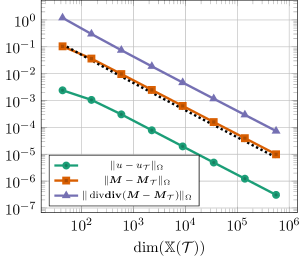
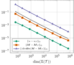
Figure 1: Errors and estimator for the smooth solution from Section 6.1; uniformly refined meshes with triangles (left) and squares (right). The black dotted line indicates $\mathcal{O}\big{(}(\#\mathcal{T})^{-1}\big{)}$.

6.2 Non-convex domain

For this experiment we consider the manufactured solution from [12, Section 6.2.2] with domain $\Omega$ as given in Figure 2. The initial triangulation with triangles is shown on the left and with parallelograms on the right. In comparison to [12, Section 6.2.2] we use a slightly modified domain that can be decomposed into triangles as well as parallelograms. The domain has a reentrant corner at the origin with interior angle $\tfrac{5}{4}\pi$. The manufactured solution is given by

$$u(x,y)=r^{1+s}\big{(}\cos((1+s)\varphi)+C\cos((1-s)\varphi)\big{)}$$

where $(r,\varphi)$ denote polar coordinates with $\varphi\in(-\pi,\pi]$. We choose $s$ and $C$ such that $u\in H^{2+s-\epsilon}(\Omega)$ ($\epsilon>0$) is a typical singularity function of the biharmonic problem with vanishing traces $u$ and $\nabla u$ on the two edges that meet at the origin. For the present case this requires to set $s\approx 0.673583$ and $C\approx 1.23459$. The singularity function satisfies (6) with $f=0$. Furthermore, note that $\widehat{\boldsymbol{u}}=\operatorname{tr}_{\Omega}^{\mathrm{Ggrad}}u\neq 0$, but $\boldsymbol{g}=\boldsymbol{M}{\boldsymbol{t}}$ is smooth on all boundary parts. Additionally, we stress that $\boldsymbol{M}\in\mathbb{H}^{s}(\Omega)$, but $\operatorname{\mathbf{div}}\boldsymbol{M}\neq L_{2}(\Omega)$. In view of a priori approximation results we thus expect the reduced convergence

$$\|u-u_{\mathcal{T}}\|_{\Omega}+\|\boldsymbol{M}-\boldsymbol{M}_{\mathcal{T}}\|_{\Omega}=\mathcal{O}\big{(}(\#\mathcal{T})^{-s/2}\big{)}$$

on a sequence of uniformly refined meshes. This is indeed observed in Figure 3 for triangular as well as parallelogram grids.

Employing the adaptive loop described above with bulk criterion $\theta=0.4$, we find that convergence order $\mathcal{O}\big{(}(\#\mathcal{T})^{-1}\big{)}$ is recovered, the one that we have seen before for smooth solutions on uniformly refined meshes. Figure 4 shows the estimator and errors for uniformly and adaptively refined triangulations. It illustrates the reliability and efficiency of the estimator in both cases. Finally, Figure 5 shows the triangulations generated by the adaptive loop. As expected, we observe strong refinements towards the reentrant corner.

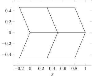
Figure 2: Domain and initial meshes for the problem from Section 6.2.

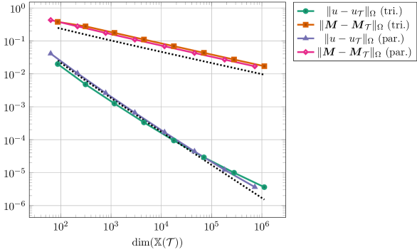
Figure 3: Errors for the singular problem from Section 6.2 on sequences of uniformly refined triangular and parallelogram meshes. The two black dotted lines indicate $\mathcal{O}\big{(}(\#\mathcal{T})^{-1}\big{)}$ and $\mathcal{O}\big{(}(\#\mathcal{T})^{-0.337}\big{)}$.

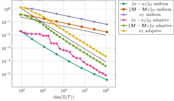
Figure 4: Errors for the singular problem from Section 6.2 on sequences of uniformly and adaptively refined triangular meshes. The two black dotted lines indicate $\mathcal{O}\big{(}(\#\mathcal{T})^{-1}\big{)}$ and $\mathcal{O}\big{(}(\#\mathcal{T})^{-0.337}\big{)}$.

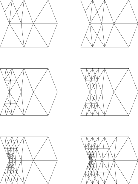
Figure 5: Meshes $\mathcal{T}_{1},\ldots,\mathcal{T}_{6}$ generated by the adaptive loop for the problem from Section 6.2. Axes are not scaled uniformly for presentation purposes.

Appendix A Basis functions

A.1 Basis functions for $\mathbb{X}_{\triangle}(K)$

In this section we construct a basis for the local space $\mathbb{X}(K)$ on a triangle $K$. Recall that $\widehat{K}=\widehat{K}_{\triangle}$ is the reference element with vertices $\widehat{z}_{1}=(0,0)$, $\widehat{z}_{2}=(1,0)$, $\widehat{z}_{3}=(0,1)$, and edges $\widehat{E}_{j}$ spanned by $\widehat{z}_{j}$, $\widehat{z}_{j+1}$. We use cyclic indexing, i.e., $\widehat{z}_{j+3}=\widehat{z}_{j}$. For the physical element we use the analogous notation without $\widehat{(\cdot)}$. We denote by $\widehat{}{\boldsymbol{t}}_{j}$ tangential vectors (positive orientation), and $\widehat{}{\boldsymbol{n}}_{j}$ are the normal vectors on edge $\widehat{E}_{j}$. Furthermore, $\widehat{\eta}_{j}$, $\eta_{j}$ denote the barycentric coordinate functions.

Defining

$$\widehat{\boldsymbol{T}}^{\triangle}_{(1,0)} =\begin{pmatrix}-x^{2}y&-xy(y-1)\\ -xy(y-1)&-y(y-1)^{2}\end{pmatrix}, \widehat{\boldsymbol{T}}^{\triangle}_{(1,1)}=\begin{pmatrix}x^{2}(2x+y-2)&x(2xy-2y-x+y^{2}+1)\\ x(2xy-2y-x+y^{2}+1)&y(y-1)(2x+y-1)\end{pmatrix},$$

$$\widehat{\boldsymbol{T}}^{\triangle}_{(2,0)} =\begin{pmatrix}x^{2}(x+y-1)&xy(x+y-1)\\ xy(x+y-1)&y^{2}(x+y-1)\end{pmatrix}, \widehat{\boldsymbol{T}}^{\triangle}_{(2,1)}=\begin{pmatrix}x^{2}(y-x+1)&-xy(x-y)\\ -xy(x-y)&-y^{2}(x-y+1)\end{pmatrix},$$

$$\widehat{\boldsymbol{T}}^{\triangle}_{(3,0)} =\begin{pmatrix}-x(x-1)^{2}&-xy(x-1)\\ -xy(x-1)&-xy^{2}\end{pmatrix}, \widehat{\boldsymbol{T}}^{\triangle}_{(3,1)}=\begin{pmatrix}-x(x-1)(x+2y-1)&-y(2xy-y-2x+x^{2}+1)\\ -y(2xy-y-2x+x^{2}+1)&-y^{2}(x+2y-2)\end{pmatrix}$$

one verifies that

$$\langle\operatorname{tr}_{\widehat{K},\widehat{E}_{\ell},{\boldsymbol{t}}}^{\mathrm{dDiv}}\widehat{\boldsymbol{T}}^{\triangle}_{(j,k)}\hskip 1.42262pt,\ell_{\widehat{E}_{\ell},m}\rangle_{\widehat{E}_{\ell}}=\delta_{j,\ell}\delta_{k,m}\quad\text{and}\quad\widehat{\boldsymbol{T}}^{\triangle}_{(j,k)}(\widehat{z}_{\ell})=0=\operatorname{tr}_{\widehat{K},\widehat{E}_{\ell},{\boldsymbol{n}}}^{\mathrm{dDiv}}\widehat{\boldsymbol{T}}^{\triangle}_{(j,k)}.$$

Lemma 17.

The transformed tensors $\boldsymbol{T}^{\triangle}_{(j,k)}=\mathcal{H}_{K}(\widehat{\boldsymbol{T}}^{\triangle}_{(j,k)})\in\mathbb{X}(K)$ satisfy

$$\langle\operatorname{tr}_{K,E_{\ell},{\boldsymbol{t}}}^{\mathrm{dDiv}}\boldsymbol{T}^{\triangle}_{(j,k)}\hskip 1.42262pt,\ell_{E_{\ell},m}\rangle_{E_{\ell}}=\delta_{j,\ell}\delta_{k,m}\quad\text{and}\quad\boldsymbol{T}^{\triangle}_{(j,k)}(z_{\ell})=0=\operatorname{tr}_{K,E_{\ell},{\boldsymbol{n}}}^{\mathrm{dDiv}}\boldsymbol{T}^{\triangle}_{(j,k)}.$$

Proof.

With $\widehat{\boldsymbol{T}}^{\triangle}_{j,k}(\widehat{z}_{\ell})=0$ it follows that $\boldsymbol{T}^{\triangle}_{j,k}(z_{\ell})=0$ by definition of the transformation.

Next, we show that $\operatorname{tr}_{K,E_{\ell},{\boldsymbol{n}}}^{\mathrm{dDiv}}\boldsymbol{T}^{\triangle}_{(j,k)}=0$. Let $\ell=1$ and $p\in P^{1}(E)$. Take $v\in H^{2}(K)$ with $v|_{\partial K}=0$, $\partial_{{\boldsymbol{n}}}v|_{E_{1}}=\eta_{E_{1}}p$, $\partial_{{\boldsymbol{n}}}v|_{E_{m}}=0$ for $m=2,3$. Note that $\eta_{E_{1}}=\eta_{1}\eta_{2}$ is the edge bubble function. Then,

$$-\langle\operatorname{tr}_{K,E_{1},{\boldsymbol{n}}}^{\mathrm{dDiv}}\boldsymbol{T}^{\triangle}_{(j,k)}\hskip 1.42262pt,\partial_{\boldsymbol{n}}v\rangle_{E_{1}} =\langle\operatorname{tr}_{K}^{\mathrm{dDiv}}\boldsymbol{T}^{\triangle}_{(j,k)}\hskip 1.42262pt,v\rangle_{\partial K}=\langle\operatorname{tr}_{\widehat{K}}^{\mathrm{dDiv}}\widehat{\boldsymbol{T}}^{\triangle}_{(j,k)}\hskip 1.42262pt,\widehat{v}\rangle_{\partial\widehat{K}}=0.$$

The latter identity follows because $\widehat{v}|_{\partial\widehat{K}}=(v\circ F_{K})|_{\partial\widehat{K}}=0$ and $\operatorname{tr}_{\widehat{K},\widehat{E}_{m},{\boldsymbol{n}}}^{\mathrm{dDiv}}\widehat{\boldsymbol{T}}^{\triangle}_{(j,k)}=0$. Since $p\in P^{1}(E_{1})$ and $\operatorname{tr}_{K,E_{1},{\boldsymbol{n}}}^{\mathrm{dDiv}}\boldsymbol{T}^{\triangle}_{(j,k)}\in P^{1}(E)$ we conclude that $\operatorname{tr}_{K,E_{1},{\boldsymbol{n}}}^{\mathrm{dDiv}}\boldsymbol{T}^{\triangle}_{(j,k)}=0$. For $\ell=2,3$ one argues similarly.

It remains to prove that $\langle\operatorname{tr}_{K,E_{\ell},{\boldsymbol{t}}}^{\mathrm{dDiv}}\boldsymbol{T}^{\triangle}_{(j,k)}\hskip 1.42262pt,\ell_{E_{\ell},m}\rangle_{E_{\ell}}=\delta_{j,\ell}\delta_{k,m}$. Let $\ell=1$. Let $p_{m}\in P^{1}(K)$ be such that $v_{m}=\eta_{E_{1}}p_{m}$ satisfies $\langle\ell_{E_{1},k}\hskip 1.42262pt,v_{m}\rangle_{E_{1}}=\langle\ell_{E_{1},k}\hskip 1.42262pt,\ell_{E_{1},m}\rangle_{E_{1}}$ for all $k,m\in\{0,1\}$. It follows that $\langle q\hskip 1.42262pt,v_{m}\rangle_{E_{1}}=\langle q\hskip 1.42262pt,\ell_{E_{1},m}\rangle_{E_{1}}$ for all $q\in P^{1}(E_{1})$ and $\langle\widehat{q}\hskip 1.42262pt,\widehat{v}_{m}\rangle_{\widehat{E}_{1}}=\langle\widehat{q}\hskip 1.42262pt,\ell_{\widehat{E}_{1},m}\rangle_{\widehat{E}_{1}}$ for all $\widehat{q}\in P^{1}(\widehat{E}_{1})$ with $\widehat{v}_{m}=v_{m}\circ F_{K}$. Then,

$$\langle\operatorname{tr}_{K,E_{1},{\boldsymbol{t}}}^{\mathrm{dDiv}}\boldsymbol{T}^{\triangle}_{(j,k)}\hskip 1.42262pt,\ell_{E_{1},m}\rangle_{E_{1}} =\langle\operatorname{tr}_{K,E_{1},{\boldsymbol{t}}}^{\mathrm{dDiv}}\boldsymbol{T}^{\triangle}_{(j,k)}\hskip 1.42262pt,v_{m}\rangle_{E_{1}}=\langle\operatorname{tr}_{K}^{\mathrm{dDiv}}\boldsymbol{T}^{\triangle}_{(j,k)}\hskip 1.42262pt,v_{m}\rangle_{\partial K}$$

$$=\langle\operatorname{tr}_{\widehat{K}}^{\mathrm{dDiv}}\widehat{\boldsymbol{T}}^{\triangle}_{(j,k)}\hskip 1.42262pt,\widehat{v}_{m}\rangle_{\partial\widehat{K}}=\langle\operatorname{tr}_{\widehat{K},\widehat{E}_{1},{\boldsymbol{t}}}^{\mathrm{dDiv}}\widehat{\boldsymbol{T}}^{\triangle}_{(j,k)}\hskip 1.42262pt,\widehat{v}_{m}\rangle_{\widehat{E}_{1}}$$

$$=\langle\operatorname{tr}_{\widehat{K},\widehat{E}_{1},{\boldsymbol{t}}}^{\mathrm{dDiv}}\widehat{\boldsymbol{T}}^{\triangle}_{(j,k)}\hskip 1.42262pt,\ell_{\widehat{E}_{1},m}\rangle_{\widehat{E}_{1}}=\delta_{j,1}\delta_{k,m}.$$

For $\ell=2,3$ one argues similarly, which finishes the proof. ∎

For the basis functions associated to jump degrees of freedom we define

$$\widetilde{\boldsymbol{J}}^{\triangle}_{j}=\frac{2}{\widehat{}{\boldsymbol{t}}_{j}\cdot\widehat{}{\boldsymbol{n}}_{j+2}-\widehat{}{\boldsymbol{t}}_{j+2}\cdot\widehat{}{\boldsymbol{n}}_{j}}\operatorname{sym}(\widehat{}{\boldsymbol{t}}_{j}\widehat{}{\boldsymbol{t}}_{j+2}^{\top})\widehat{\eta}_{j}.$$

One verifies that $[{\boldsymbol{t}}\cdot\widetilde{\boldsymbol{J}}^{\triangle}_{j}{\boldsymbol{n}}]_{\partial\widehat{K}}(\widehat{z}_{k})=\delta_{j,k}$ and $\operatorname{tr}_{\widehat{K},\widehat{E}_{k},{\boldsymbol{n}}}^{\mathrm{dDiv}}\widetilde{\boldsymbol{J}}^{\triangle}_{j}=0$. However, the traces $\operatorname{tr}_{\widehat{K},\widehat{E}_{k},{\boldsymbol{t}}}^{\mathrm{dDiv}}\widetilde{\boldsymbol{J}}^{\triangle}_{j}$ do not vanish on all edges. To overcome this we subtract some correction terms:

$$\widehat{\boldsymbol{J}}^{\triangle}_{j}:=\widetilde{\boldsymbol{J}}^{\triangle}_{j}-\sum_{\ell=1}^{3}\langle\operatorname{tr}_{\widehat{K},\widehat{E}_{\ell},{\boldsymbol{t}}}^{\mathrm{dDiv}}\widetilde{\boldsymbol{J}}^{\triangle}_{j}\hskip 1.42262pt,1\rangle_{\widehat{E}_{\ell}}\widehat{\boldsymbol{T}}^{\triangle}_{\ell,0}.$$

Lemma 18.

The transformed tensors $\boldsymbol{J}^{\triangle}_{j}=\mathcal{H}_{K}(\widehat{\boldsymbol{J}}^{\triangle}_{j})\in\mathbb{X}(K)$ satisfy

$$\operatorname{tr}_{K,E_{\ell},{\boldsymbol{n}}}^{\mathrm{dDiv}}\boldsymbol{J}^{\triangle}_{j}=0=\operatorname{tr}_{K,E_{\ell},{\boldsymbol{t}}}^{\mathrm{dDiv}}\boldsymbol{J}^{\triangle}_{j}\quad\text{and}\quad[{\boldsymbol{t}}\cdot\boldsymbol{J}^{\triangle}_{j}{\boldsymbol{n}}]_{\partial K}(z_{k})=\delta_{j,k}.$$

Proof.

The identities $\operatorname{tr}_{K,E_{\ell},{\boldsymbol{n}}}^{\mathrm{dDiv}}\boldsymbol{J}^{\triangle}_{j}=0=\operatorname{tr}_{K,E_{\ell},{\boldsymbol{t}}}^{\mathrm{dDiv}}\boldsymbol{J}^{\triangle}_{j}$ can be shown as in the proof of Lemma 17. For the last identity, take $v=\eta_{k}\in H^{2}(K)$. Then,

$$-\delta_{j,k} =-[{\boldsymbol{t}}\cdot\widehat{\boldsymbol{J}}^{\triangle}_{j}{\boldsymbol{n}}]_{\partial\widehat{K}}(\widehat{z}_{k})\widehat{v}(\widehat{z}_{k})=\langle\operatorname{tr}_{\widehat{K}}^{\mathrm{dDiv}}\widehat{\boldsymbol{J}}^{\triangle}\hskip 1.42262pt,\widehat{v}\rangle_{\partial\widehat{K}}=\langle\operatorname{tr}_{K}^{\mathrm{dDiv}}\boldsymbol{J}^{\triangle}\hskip 1.42262pt,v\rangle_{\partial K}$$

$$=-[{\boldsymbol{t}}\cdot\boldsymbol{J}^{\triangle}_{j}{\boldsymbol{n}}]_{\partial K}(z_{k})v(z_{k})=-[{\boldsymbol{t}}\cdot\boldsymbol{J}^{\triangle}_{j}{\boldsymbol{n}}]_{\partial K}(z_{k}),$$

which finishes the proof. ∎

We define the remaining basis functions directly on $K$ (rather than by transformation from the reference element),

$$\widetilde{\boldsymbol{N}}^{\triangle}_{(j,0)}=\frac{1}{{\boldsymbol{t}}_{j+1}\cdot{\boldsymbol{n}}_{j}\,{\boldsymbol{t}}_{j+2}\cdot{\boldsymbol{n}}_{j}}\operatorname{sym}({\boldsymbol{t}}_{j+1}{\boldsymbol{t}}_{j+2}^{\top}),\quad\widetilde{\boldsymbol{N}}^{\triangle}_{(j,1)}=\widetilde{\boldsymbol{N}}^{\triangle}_{(j,0)}(\eta_{j+1}-\eta_{j}),\quad j=1,2,3.$$

These functions satisfy $\operatorname{tr}_{K,E_{\ell},{\boldsymbol{n}}}^{\mathrm{dDiv}}\widetilde{\boldsymbol{N}}^{\triangle}_{(j,k)}=\delta_{j,\ell}\ell_{E_{j},k}$ but the other trace terms do not vanish in general. As before we subtract correction terms and define

$$\boldsymbol{N}^{\triangle}_{(j,0)} =\widetilde{\boldsymbol{N}}^{\triangle}_{(j,0)}-\sum_{\ell=1}^{3}[{\boldsymbol{t}}\cdot\widetilde{\boldsymbol{N}}^{\triangle}_{(j,0)}{\boldsymbol{n}}]_{\partial K}(z_{\ell})\boldsymbol{J}^{\triangle}_{\ell},$$

$$\boldsymbol{N}^{\triangle}_{(j,1)} =\widetilde{\boldsymbol{N}}^{\triangle}_{(j,1)}-\sum_{\ell=1}^{3}\langle\operatorname{tr}_{K,E_{\ell},{\boldsymbol{t}}}^{\mathrm{dDiv}}\widetilde{\boldsymbol{N}}^{\triangle}_{(j,1)}\hskip 1.42262pt,1\rangle_{E_{\ell}}\boldsymbol{T}^{\triangle}_{(\ell,0)}-\sum_{\ell=1}^{3}[{\boldsymbol{t}}\cdot\widetilde{\boldsymbol{N}}^{\triangle}_{(j,1)}{\boldsymbol{n}}]_{\partial K}(z_{\ell})\boldsymbol{J}^{\triangle}_{\ell}.$$

In the following lemma we collect some properties.

Lemma 19.

The tensors $\boldsymbol{N}^{\triangle}_{(j,k)}\in\mathbb{X}(K)$ satisfy

$$\operatorname{tr}_{K,E_{\ell},{\boldsymbol{t}}}^{\mathrm{dDiv}}\boldsymbol{N}^{\triangle}_{(j,k)}=0=[{\boldsymbol{t}}\cdot\boldsymbol{N}^{\triangle}_{j}{\boldsymbol{n}}]_{\partial K}(z_{k})\quad\text{and}\quad\operatorname{tr}_{K,E_{\ell},{\boldsymbol{n}}}^{\mathrm{dDiv}}\boldsymbol{N}^{\triangle}_{(j,k)}=\delta_{j,\ell}\ell_{E_{j},k}.$$

Furthermore,

$$\boldsymbol{N}^{\triangle}_{(j,1)}=\widetilde{\boldsymbol{N}}^{\triangle}_{(j,1)}-\sum_{\ell=1}^{3}[{\boldsymbol{t}}\cdot\widetilde{\boldsymbol{N}}^{\triangle}_{(j,1)}{\boldsymbol{n}}]_{\partial K}(z_{\ell})\widetilde{\boldsymbol{J}}^{\triangle,K}_{\ell}\in\mathbb{P}_{\mathrm{sym}}^{1}(K)$$

where

$$\widetilde{\boldsymbol{J}}_{\ell}^{\triangle,K}=\frac{2}{{\boldsymbol{t}}_{j}\cdot{\boldsymbol{n}}_{j+2}-{\boldsymbol{t}}_{j+2}\cdot{\boldsymbol{n}}_{j}}\operatorname{sym}({\boldsymbol{t}}_{j}{\boldsymbol{t}}_{j+2}^{\top})\eta_{j}.$$

Proof.

All but the last assertion follow by construction. To see the last assertion we note that $\widetilde{\boldsymbol{J}}^{\triangle,K}_{j}$ is constructed as $\widetilde{\boldsymbol{J}}^{\triangle}_{j}$ but now on the element $K$ instead of $\widehat{K}$. As before one verifies that $[{\boldsymbol{t}}\cdot\widetilde{\boldsymbol{J}}^{\triangle,K}_{j}{\boldsymbol{n}}]_{\partial K}(z_{k})=\delta_{j,k}$ and $\operatorname{tr}_{K,E_{k},{\boldsymbol{n}}}^{\mathrm{dDiv}}\widetilde{\boldsymbol{J}}^{\triangle,K}_{j}=0$. Set

$$\overline{\boldsymbol{N}}^{\triangle}_{(j,1)}=\widetilde{\boldsymbol{N}}^{\triangle}_{(j,1)}-\sum_{\ell=1}^{3}[{\boldsymbol{t}}\cdot\widetilde{\boldsymbol{N}}^{\triangle}_{(j,1)}{\boldsymbol{n}}]_{\partial K}(z_{\ell})\widetilde{\boldsymbol{J}}^{\triangle,K}_{\ell}.$$

The proof is finished if we show that $\overline{\boldsymbol{N}}^{\triangle}_{(j,1)}=\boldsymbol{N}^{\triangle}_{(j,1)}$. First, note that $\operatorname{tr}_{K,E_{k},{\boldsymbol{n}}}^{\mathrm{dDiv}}\overline{\boldsymbol{N}}^{\triangle}_{(j,1)}=\operatorname{tr}_{K,E_{k},{\boldsymbol{n}}}^{\mathrm{dDiv}}\boldsymbol{N}^{\triangle}_{(j,1)}$. Second, $[{\boldsymbol{t}}\cdot\overline{\boldsymbol{N}}^{\triangle}_{(j,1)}{\boldsymbol{n}}]_{\partial K}(z_{k})=0$. Finally, $\operatorname{tr}_{K,E_{k},{\boldsymbol{t}}}^{\mathrm{dDiv}}\overline{\boldsymbol{N}}^{\triangle}_{(j,1)}=0$ follows from a straightforward and simple but rather lengthy calculation (not shown). ∎

The following theorem summarizes the results of this section.

Theorem 20.

The elements of $\mathbb{B}:=\{\boldsymbol{N}^{\triangle}_{(j,k)},\boldsymbol{T}^{\triangle}_{(j,k)},\boldsymbol{J}^{\triangle}_{j}\,:\,j=1,2,3,\,k=0,1\}$ define a basis of $\mathbb{X}(K)$ and are dual to the degrees of freedom (3). Moreover,

$$\|\boldsymbol{B}\|_{K}\eqsim h_{K}\quad\forall\boldsymbol{B}\in\mathbb{B}.$$

Proof.

By construction the elements of $\mathbb{B}$ are dual to the degrees of freedom (3) and $\mathbb{B}\subset\mathbb{X}(K)$. We conclude that $\mathbb{B}$ is a basis of $\mathbb{X}(K)$. For the scaling properties we note that $\boldsymbol{T}^{\triangle}_{(j,k)}$ and $\boldsymbol{J}^{\triangle}_{j}$ have been defined through the Piola–Kirchhoff transformation and by Lemma 3 we get

$$\|\boldsymbol{T}^{\triangle}_{(j,k)}\|_{K}\eqsim h_{K}\|\widehat{\boldsymbol{T}}^{\triangle}_{(j,k)}\|_{K}\eqsim h_{K}\quad\text{and}\quad\|\boldsymbol{J}^{\triangle}_{j}\|_{K}\eqsim h_{K}\|\widehat{\boldsymbol{J}}^{\triangle}_{j}\|_{K}\eqsim h_{K}.$$

To see that $\|\boldsymbol{N}^{\triangle}_{(j,k)}\|_{K}\eqsim h_{K}$ set $\alpha_{(j,k),\ell}=[{\boldsymbol{t}}\cdot\widetilde{\boldsymbol{N}}_{(j,k)}^{\triangle}{\boldsymbol{n}}](z_{\ell})$ and observe that $\sum_{\ell=1}^{3}|\alpha_{(j,k),\ell}|\lesssim C$ with $C>0$ a generic constant independent of $h_{K}$, $j$ and $k$. Standard scaling arguments then show

$$\|\boldsymbol{N}_{(j,k)}^{\triangle}\|_{K}\eqsim h_{K}\|\mathcal{H}_{K}^{-1}\boldsymbol{N}_{(j,k)}^{\triangle}\|_{\widehat{K}}\eqsim h_{K}\big{(}1+\sum_{\ell=1}^{3}|\alpha_{(j,k),\ell}|\big{)}\eqsim h_{K},$$

which finishes the proof. ∎

A.2 Basis functions for $\mathbb{X}_{\square}(K)$

In this section we construct a basis of the local space $\mathbb{X}(K)$ for a parallelogram $K$. Recall that $\widehat{K}=\widehat{K}_{\square}$ is the reference element with vertices $\widehat{z}_{1}=(0,0)$, $\widehat{z}_{2}=(1,0)$, $\widehat{z}_{3}=(1,1)$, $\widehat{z}_{4}=(0,1)$ and edges $\widehat{E}_{j}$ spanned by $\widehat{z}_{j}$, $\widehat{z}_{j+1}$. We adopt the notation from Section A.1 with obvious modifications. A slight difference is that here $\widehat{\eta}_{j}$ denotes the bilinear function on the reference element with $\eta_{j}(z_{k})=\delta_{jk}$ and $\eta_{j}\circ F_{K}=\widehat{\eta}_{j}$.

Defining

$$\widehat{\boldsymbol{T}}^{\square}_{(1,0)} =\begin{pmatrix}x(2y-1)(x-1)/4&-y(2x-1)(y-1)/8\\ -y(2x-1)(y-1)/8&-y(y-1)^{2}\end{pmatrix}, \widehat{\boldsymbol{T}}^{\square}_{(1,1)}=\begin{pmatrix}0&3x(2y-3)(x-1)/8\\ 3x(2y-3)(x-1)/8&3y(2x-1)(y-1)/4\end{pmatrix},$$

$$\widehat{\boldsymbol{T}}^{\square}_{(2,0)} =\begin{pmatrix}x^{2}(x-1)&x(2y-1)(x-1)/8\\ x(2y-1)(x-1)/8&-y(2x-1)(y-1)/4\end{pmatrix}, \widehat{\boldsymbol{T}}^{\square}_{(2,1)}=\begin{pmatrix}3x(2y-1)(x-1)/4&3y(2x+1)(y-1)/8\\ 3y(2x+1)(y-1)/8&0\end{pmatrix},$$

$$\widehat{\boldsymbol{T}}^{\square}_{(3,0)} =\begin{pmatrix}-x(2y-1)(x-1)/4&y(2x-1)(y-1)/8\\ y(2x-1)(y-1)/8&y^{2}(y-1)\end{pmatrix}, \widehat{\boldsymbol{T}}^{\square}_{(3,1)}=\begin{pmatrix}0&-3x(2y+1)(x-1)/8\\ -3x(2y+1)(x-1)/8&-3y(2x-1)(y-1)/4\end{pmatrix},$$

$$\widehat{\boldsymbol{T}}^{\square}_{(4,0)} =\begin{pmatrix}-x(x-1)^{2}&-x(2y-1)(x-1)/8\\ -x(2y-1)(x-1)/8&y(2x-1)(y-1)/4\end{pmatrix}, \widehat{\boldsymbol{T}}^{\square}_{(4,1)}=\begin{pmatrix}-3x(2y-1)(x-1)/4&-3y(2x-3)(y-1)/8\\ -3y(2x-3)(y-1)/8&0\end{pmatrix}$$

one verifies that

$$\langle\operatorname{tr}_{\widehat{K},\widehat{E}_{\ell},{\boldsymbol{t}}}^{\mathrm{dDiv}}\widehat{\boldsymbol{T}}^{\square}_{(j,k)}\hskip 1.42262pt,\ell_{\widehat{E}_{\ell},m}\rangle_{\widehat{E}_{\ell}}=\delta_{j,\ell}\delta_{k,m}\quad\text{and}\quad\widehat{\boldsymbol{T}}^{\square}_{(j,k)}(\widehat{z}_{\ell})=0=\operatorname{tr}_{\widehat{K},\widehat{E}_{\ell},{\boldsymbol{n}}}^{\mathrm{dDiv}}\widehat{\boldsymbol{T}}^{\square}_{(j,k)}.$$

Lemma 21.

The transformed tensors $\boldsymbol{T}^{\square}_{(j,k)}=\mathcal{H}_{K}(\widehat{\boldsymbol{T}}^{\square}_{(j,k)})\in\mathbb{X}(K)$ satisfy

$$\langle\operatorname{tr}_{K,E_{\ell},{\boldsymbol{t}}}^{\mathrm{dDiv}}\boldsymbol{T}^{\square}_{(j,k)}\hskip 1.42262pt,\ell_{E_{\ell},m}\rangle_{E_{\ell}}=\delta_{j,\ell}\delta_{k,m}\quad\text{and}\quad\boldsymbol{T}^{\square}_{(j,k)}(z_{\ell})=0=\operatorname{tr}_{K,E_{\ell},{\boldsymbol{n}}}^{\mathrm{dDiv}}\boldsymbol{T}^{\square}_{(j,k)}.$$

Proof.

The proof follows along the lines of the proof of Lemma 17 and is therefore omitted. ∎

For the basis functions associated to jump degrees of freedom we define

$$\widetilde{\boldsymbol{J}}^{\square}_{j}=\operatorname{sym}(\widehat{}{\boldsymbol{t}}_{j}\widehat{}{\boldsymbol{t}}_{j+1}^{\top})\widehat{\eta}_{j}=\frac{(-1)^{j}}{2}\widehat{\eta}_{j}\begin{pmatrix}0&1\\ 1&0\end{pmatrix}.$$

One verifies that $[{\boldsymbol{t}}\cdot\widetilde{\boldsymbol{J}}^{\square}_{j}{\boldsymbol{n}}]_{\partial\widehat{K}}(\widehat{z}_{k})=\delta_{j,k}$ and $\operatorname{tr}_{\widehat{K},\widehat{E}_{k},{\boldsymbol{n}}}^{\mathrm{dDiv}}\widetilde{\boldsymbol{J}}^{\square}_{j}=0$. However, the traces $\operatorname{tr}_{\widehat{K},\widehat{E}_{k},{\boldsymbol{t}}}^{\mathrm{dDiv}}\widetilde{\boldsymbol{J}}^{\square}_{j}$ do not vanish on all edges. As in the previous section we subtract correction terms

$$\widehat{\boldsymbol{J}}^{\square}_{j}:=\widetilde{\boldsymbol{J}}^{\square}_{j}-\sum_{\ell=1}^{4}\langle\operatorname{tr}_{\widehat{K},\widehat{E}_{\ell},{\boldsymbol{t}}}^{\mathrm{dDiv}}\widetilde{\boldsymbol{J}}^{\square}_{j}\hskip 1.42262pt,1\rangle_{\widehat{E}_{\ell}}\widehat{\boldsymbol{T}}^{\square}_{(\ell,0)}=\widetilde{\boldsymbol{J}}^{\square}_{j}-\widehat{\boldsymbol{T}}^{\square}_{(j-1,0)}-\widehat{\boldsymbol{T}}^{\square}_{(j,0)}.$$

Lemma 22.

The transformed tensors $\boldsymbol{J}^{\square}_{j}=\mathcal{H}_{K}(\widehat{\boldsymbol{J}}^{\square}_{j})\in\mathbb{X}(K)$ satisfy

$$\operatorname{tr}_{K,E_{\ell},{\boldsymbol{n}}}^{\mathrm{dDiv}}\boldsymbol{J}^{\square}_{j}=0=\operatorname{tr}_{K,E_{\ell},{\boldsymbol{t}}}^{\mathrm{dDiv}}\boldsymbol{J}^{\square}_{j}\quad\text{and}\quad[{\boldsymbol{t}}\cdot\boldsymbol{J}^{\square}_{j}{\boldsymbol{n}}]_{\partial K}(z_{k})=\delta_{j,k}.$$

Proof.

We only have to prove that $\boldsymbol{J}^{\square}_{j}\in\mathbb{X}(K)$. The proof of the other assertions follows along the lines of the proof of Lemma 18 and is therefore omitted. Let $\mathbb{Q}^{1}(\widehat{K})\subset\mathbb{P}_{\mathrm{sym}}^{2}(\widehat{K})$ denote the space of symmetric tensor-valued polynomials with bilinear components. From the definition of $\mathbb{X}(\widehat{K})$ we find that $\mathbb{Q}^{1}(\widehat{K})\subset\mathbb{X}(\widehat{K})$. Noting that $\widetilde{\boldsymbol{J}}_{j}^{\square}\in\mathbb{Q}^{1}(\widehat{K})$ we conclude that $\mathcal{H}_{K}\widetilde{\boldsymbol{J}}_{j}^{\square}\in\mathbb{X}(K)$ by Proposition 6, and, consequently, $\boldsymbol{J}_{j}^{\square}\in\mathbb{X}(K)$. ∎

As in the previous section, the remaining basis functions are defined directly on the physical element $K$,

$$\widetilde{\boldsymbol{N}}^{\square}_{(j,0)}=\frac{1}{|{\boldsymbol{t}}_{j+1}\cdot{\boldsymbol{n}}_{j}|^{2}}{\boldsymbol{t}}_{j+1}{\boldsymbol{t}}_{j+1}^{\top}(\eta_{j}+\eta_{j+1}),\quad\widetilde{\boldsymbol{N}}^{\square}_{(j,1)}=\frac{1}{|{\boldsymbol{t}}_{j+1}\cdot{\boldsymbol{n}}_{j}|^{2}}{\boldsymbol{t}}_{j+1}{\boldsymbol{t}}_{j+1}^{\top}(\eta_{j+1}-\eta_{j}).$$

By construction these functions satisfy $\operatorname{tr}_{K,E_{\ell},{\boldsymbol{n}}}^{\mathrm{dDiv}}\widetilde{\boldsymbol{N}}^{\square}_{(j,k)}=\delta_{j,\ell}\ell_{E_{j},k}$. As before we subtract correction terms to ensure that the other trace terms vanish,

$$\boldsymbol{N}^{\square}_{(j,0)} =\widetilde{\boldsymbol{N}}^{\square}_{(j,0)}-\sum_{\ell=1}^{4}\sum_{k=0}^{1}\langle\operatorname{tr}_{K,E,{\boldsymbol{t}}}^{\mathrm{dDiv}}\widetilde{\boldsymbol{N}}^{\square}_{(j,0)}\hskip 1.42262pt,\ell_{E_{\ell},k}\rangle_{E_{\ell}}\boldsymbol{T}^{\square}_{(\ell,k)}-\sum_{\ell=1}^{4}[{\boldsymbol{t}}\cdot\widetilde{\boldsymbol{N}}^{\square}_{(j,0)}{\boldsymbol{n}}]_{\partial K}(z_{\ell})\boldsymbol{J}^{\square}_{\ell},$$

$$\boldsymbol{N}^{\square}_{(j,1)} =\widetilde{\boldsymbol{N}}^{\square}_{(j,1)}-\sum_{\ell=1}^{4}\sum_{k=0}^{1}\langle\operatorname{tr}_{K,E,{\boldsymbol{t}}}^{\mathrm{dDiv}}\widetilde{\boldsymbol{N}}^{\square}_{(j,1)}\hskip 1.42262pt,\ell_{E_{\ell},k}\rangle_{E_{\ell}}\boldsymbol{T}^{\square}_{(\ell,k)}-\sum_{\ell=1}^{4}[{\boldsymbol{t}}\cdot\widetilde{\boldsymbol{N}}^{\square}_{(j,1)}{\boldsymbol{n}}]_{\partial K}(z_{\ell})\boldsymbol{J}^{\square}_{\ell}.$$

In the following lemma we collect some properties.

Lemma 23.

Tensors $\boldsymbol{N}^{\square}_{(j,k)}\in\mathbb{X}(K)$ satisfy

$$\operatorname{tr}_{K,E_{\ell},{\boldsymbol{t}}}^{\mathrm{dDiv}}\boldsymbol{N}^{\square}_{(j,k)}=0=[{\boldsymbol{t}}\cdot\boldsymbol{N}^{\square}_{j}{\boldsymbol{n}}]_{\partial K}(z_{k})\quad\text{and}\quad\operatorname{tr}_{K,E_{\ell},{\boldsymbol{n}}}^{\mathrm{dDiv}}\boldsymbol{N}^{\square}_{(j,k)}=\delta_{j,\ell}\ell_{E_{j},k}.$$

Proof.

We only have to show that $\boldsymbol{N}^{\square}_{(j,k)}\in\mathbb{X}(K)$. The remaining assertions follow by definition. Using the space of symmetric, bilinear tensors $\mathbb{Q}^{1}(\widehat{K})$ from before, we note that $\mathcal{H}_{K}^{-1}\widetilde{\boldsymbol{N}}^{\square}_{(j,k)}\in\mathbb{Q}^{1}(\widehat{K})$. It follows that $\widetilde{\boldsymbol{N}}^{\square}_{(j,k)}\in\mathbb{X}(K)$ by Proposition 6. We conclude that $\boldsymbol{N}^{\square}_{(j,k)}\in\mathbb{X}(K)$. ∎

Theorem 24.

The elements of $\mathbb{B}:=\{\boldsymbol{N}^{\square}_{(j,k)},\boldsymbol{T}^{\square}_{(j,k)},\boldsymbol{J}^{\square}_{j}\,:\,j=1,2,3,\,k=0,1\}$ define a basis of $\mathbb{X}(K)$ and are dual to the degrees of freedom (3). Moreover,

$$\|\boldsymbol{B}\|_{K}\eqsim h_{K}\quad\forall\boldsymbol{B}\in\mathbb{B}.$$

Proof.

The proof follows as for Theorem 20 and is therefore omitted. ∎

References

- [1] H. Blum and R. Rannacher, On the boundary value problem of the biharmonic operator on domains with angular corners, Math. Methods Appl. Sci., 2 (1980), pp. 556–581.
- [2] D. Boffi, F. Brezzi, and M. Fortin, Mixed finite element methods and applications, vol. 44 of Springer Series in Computational Mathematics, Springer, Heidelberg, 2013.
- [3] J. H. Bramble and R. S. Falk, Two mixed finite element methods for the simply supported plate problem, RAIRO Anal. Numér., 17 (1983), pp. 337–384.
- [4] C. Carstensen, A posteriori error estimate for the mixed finite element method, Math. Comp., 66 (1997), pp. 465–476.
- [5] L. Chen and X. Huang, Finite elements for -conforming symmetric tensors, arXiv:2005.01271, 2021.
- [6] , A mixed finite element method for the biharmonic equation with hybridization, arXiv, arXiv:2305.11356 (2023).
- [7] P. G. Ciarlet and P.-A. Raviart, A mixed finite element method for the biharmonic equation, Math. Res. Center, Univ. of Wisconsin-Madison, Academic Press, New York, 1974, pp. 125–145. Publication No. 33.
- [8] P. Clément, Approximation by finite element functions using local regularization, Rev. Française Automat. Informat. Recherche Opérationnelle Sér., 9 (1975), pp. 77–84.
- [9] R. S. Falk, Approximation of the biharmonic equation by a mixed finite element method, SIAM J. Numer. Anal., 15 (1978), pp. 556–567.
- [10] T. Führer, A. Haberl, and N. Heuer, Trace operators of the bi-Laplacian and applications, IMA J. Numer. Anal., 41 (2021), pp. 1031–1055.
- [11] T. Führer and N. Heuer, Fully discrete DPG methods for the Kirchhoff-Love plate bending model, Comput. Methods Appl. Mech. Engrg., 343 (2019), pp. 550–571.
- [12] T. Führer, N. Heuer, and A. H. Niemi, An ultraweak formulation of the Kirchhoff-Love plate bending model and DPG approximation, Math. Comp., 88 (2019), pp. 1587–1619.
- [13] G. N. Gatica, A simple introduction to the mixed finite element method, SpringerBriefs in Mathematics, Springer, Cham, 2014. Theory and applications.
- [14] P. Grisvard, Elliptic problems in nonsmooth domains, vol. 24 of Monographs and Studies in Mathematics, Pitman (Advanced Publishing Program), Boston, MA, 1985.
- [15] K. Hellan, Analysis of elastic plates in flexure by a simplified finite element method, Acta Polytech. Scand. Civ. Eng. Build. Constr. Ser. 46, 1 (1967).
- [16] L. R. Herrmann, Finite-element bending analysis for plates, J. Eng. Mech. Div., 93 (1967), pp. 13–26.
- [17] J. Hu, R. Ma, and M. Zhang, A family of mixed finite elements for the biharmonic equations on triangular and tetrahedral grids, Sci. China Math., 64 (2021), pp. 2793–2816.
- [18] C. Johnson, On the convergence of a mixed finite-element method for plate bending problems, Numer. Math., 21 (1973), pp. 43–62.
- [19] P. Monk, A mixed finite element method for the biharmonic equation, SIAM J. Numer. Anal., 24 (1987), pp. 737–749.
- [20] A. Pechstein and J. Schöberl, Tangential-displacement and normal-normal-stress continuous mixed finite elements for elasticity, Math. Models Methods Appl. Sci., 21 (2011), pp. 1761–1782.
- [21] K. Rafetseder and W. Zulehner, A decomposition result for Kirchhoff plate bending problems and a new discretization approach, SIAM J. Numer. Anal., 56 (2018), pp. 1961–1986.
- [22] L. R. Scott and S. Zhang, Finite element interpolation of nonsmooth functions satisfying boundary conditions, Math. Comp., 54 (1990), pp. 483–493.
- [23] R. Verfürth, A posteriori error estimation and adaptive mesh-refinement techniques, in Proceedings of the Fifth International Congress on Computational and Applied Mathematics (Leuven, 1992), vol. 50, 1994, pp. 67–83.