Precision prediction at the LHC of a democratic up-family philic KSVZ axion model

Abstract

In this work, we study the $SU(2)_{L}$ singlet complex scalar extended KSVZ model that, in addition to providing a natural solution to the strong-CP problem by including a global Peccei-Quinn symmetry, also furnishes two components of dark matter that satisfy observer relic density without fine-tuning of model parameters. Furthermore, this model provides a rich phenomenology by introducing a vector-like quark whose presence can be sensed in collider experiments and dark matter production mechanisms. We explore the possibility of democratic Yukawa interaction of the vector-like quark with all up-type quarks and scalar dark matter candidate. We also employ next-to-leading order NLO-QCD correction for VLQ pair production to study a unique search at the LHC, generating a pair of boosted tops with sizeable missing transverse momentum. Multivariate analysis with jet substructure variables has a strong ability to explore a significant parameter space of this model at the 14 TeV LHC.

1 Introduction

The Standard Model (SM) of particle physics harbours several shortcomings despite providing the most successful theory of the underlying nature of fundamental particles and their interactions, verified in many low to high-energy experiments consistently delivering excellent agreement. Among many such issues relating to some internal inconsistencies to the inability to explain some of the observations, significant flaws like the strong-CP problem Cheng:1987gp ; Baluni:1978rf ; Dine:2000cj , the existence of dark matter (DM) Sofue:2000jx ; Clowe:2006eq , baryon-antibaryon asymmetry of the universe Riotto:1999yt ; Dine:2003ax , neutrino masses Super-Kamiokande:1998kpq ; SNO:2002tuh ; K2K:2002icj , etc. are the ones which generated lots of attention in motivating to go beyond the Standard Model (BSM) and their searches at different experiments.

The $SU(3)_{C}$ symmetry of SM allows a term like $\theta\dfrac{g_{S}^{2}}{32\pi^{2}}\tilde{G}_{\mu\nu}G^{\mu\nu}$, where $G^{\mu\nu}$ is the gluon field strength tensor. This term contributes to the neutron electric dipole moment, and the experimental measurement PhysRevLett.124.081803 constraints the parameter $\overline{\theta}\leq 10^{-10}$. These two parameters $\overline{\theta}$ and $\theta$ are related through quark field chiral rotation. Since $\overline{\theta}\rightarrow 0$ does not promote any symmetry of the theory, one would anticipate $\overline{\theta}\sim\mathcal{O}(1)$, which is known as a strong charge-parity (CP) problem Cheng:1987gp ; Baluni:1978rf ; Dine:2000cj . Roberto Peccei and Helen Quinn proposed a classic resolution to this critical issue in 1977 by extending the SM with a global Peccei-Quinn (PQ) symmetry, expected to be broken spontaneously at a scale far larger than the Electroweak (EW) scale. The breaking of $U(1)_{PQ}$ predicts the existence of a pseudo-Goldstone particle, also known as the QCD axion. It is even more interesting to note that although QCD axion is not entirely stable, it can have a lifetime comparable to the age of the Universe, thanks to the sizeable breaking scale, to play the role of dark matter Peccei:1977hh ; Peccei:1977ur . Hence such models can concurrently explain the presence of the DM in the Universe while also solving the strong-CP problem.

After breaking $U(1)_{PQ}$ symmetry, one may formulate an axion-gluon effective Lagrangian where $F_{a}$ is the Peccei-Quinn breaking scale and this Lagrangian appears to be

$$\mathcal{L}=\mathcal{L}_{\text{QCD}}+\theta\dfrac{g_{S}^{2}}{32\pi^{2}}\tilde{G}_{\mu\nu}G^{\mu\nu}+\dfrac{1}{2}\partial_{\mu}a\partial^{\mu}a-\dfrac{g_{S}^{2}}{32\pi^{2}F_{a}}a(x)\tilde{G}_{\mu\nu}G^{\mu\nu}.$$ (1)

After minimizing the axion potential, one can write $\overline{\theta}=\theta-\dfrac{1}{F_{a}}<a(x)>$. As a result, the vacuum expectation value of the axion field cancels the original $\theta$, and the strong CP issue is resolved. Among different existing models Kim-Shifman-Vainshtein-Zakharov (KSVZ) Kim:1979if ; Shifman:1979if provides some of the exciting phenomenological implementations above and over its capability to solve two of the most outstanding problems of SM. This model includes a PQ-breaking complex scalar that is singlet under the SM gauge groups $\eta\sim(1,1,0)$, as well as a vector-like quark (VLQ) $\Psi=\Psi_{L}+\Psi_{R}$ that is $SU(3)_{C}$ colour triplet but $SU(2)_{L}$ singlet with hypercharge zero, so that, $\Psi\sim(3,1,0)$. The interaction term between VLQ and the scalar is $f_{\Psi}\eta\overline{\Psi}_{L}\Psi_{R}+h.c$, where $f_{\Psi}$ is the interaction strength. The scalar field can be written as,

$$\eta=\frac{1}{\sqrt{2}}(F_{a}+\sigma_{0})~{}e^{\frac{ia(x)}{F_{a}}}.$$ (2)

Here $F_{a}$ is the PQ breaking scale, $\sigma_{0}$ and $a(x)$ are the radial mode and the axion field, respectively. Following the symmetry breaking, VLQ gains mass proportionate to the PQ breaking scale, and they are thus isolated from the axion field and may be safely integrated out. This leads to an axion-gluon effective Lagrangian (the final term of Equation 1), and the strong-CP problem is resolved. Axion can get a tiny mass (at the order of a few MeV) after QCD confinement and decay into a pair of gluons through loop-induced VLQ. Since its decay rate is inversely proportional to the PQ breaking scale, if the braking scale is tuned correctly, the axion lifetime can be larger than the age of the Universe and behaves as a DM.

It is also worth noting that the breaking of PQ symmetry in these models leaves a residual $\mathbb{Z}_{2}$ symmetry that remains intact. Axion can provide the correct relic density of DM as measured by the Planck collaboration Akrami:2018odb , but after the corresponding breaking scale is fine-tuned. We analyze an extended KSVZ model which circumvents such fine-tuning by adding another complex scalar $S\sim(1,1,0)$, a singlet under SM. Under the residual $\mathbb{Z}_{2}$ symmetry of the KSVZ model, VLQ is odd in this setup, and $S$ is likewise $\mathbb{Z}_{2}$-odd. Therefore the lightest component of $S$ serves as the second dark matter candidate. VLQ interacts with Standard Model quarks and the scalar $S$ in the present configuration. The hypercharge of VLQ is determined by the kind (up or down) of SM quarks considered.

Given that we are considering up-type quarks, the hypercharge of VLQ is $\frac{2}{3}$. VLQ plays a critical role in dark matter phenomenology because it opens up new coannihilation and annihilation channels, such as coannihilation between scalar DM and VLQ and annihilation of VLQs into SM particles, which has a significant impact on relic density calculations. Since DM interacts with the SM quarks through VLQ, additional direct detection channels open up, such as VLQ-mediated t-channel elastic scattering between the SM-quark and scalar DM. Moreover, the VLQ and its interaction with SM quarks also affect the LHC phenomenology. VLQ decays into an SM-quark and a missing DM particle after being produced at the LHC. As a result, multijet plus missing transverse momentum may be employed as a possible probe. If the mass difference between VLQ and DM is more than the top quark mass, VLQ can be probed from its decay into top quarks, along with a sizeable missing transverse energy from dark matter in the final state.

The Yukawa interaction takes the form $f_{i}S\overline{\Psi}_{L}{u_{i}}_{R}+~{}h.c$, where $u_{R}$ denotes right-handed up-type SM-quarks with $i=u,~{}c,~{}t$. We first consider the parameter spaces that yield the correct relic density and are permissible from other experimental observations such as direct detection (DD), collider data, etc., with equal (democratic) coupling strengths $f_{u}=f_{c}=f_{t}$ at all three generations. Interestingly, one would find that the flavour constraint strongly disfavours this democratic option, although such models can be allowed from observed relic density and all other constraints (please follow the flavour constraints part in Section 2). The flavour constraint requires either or both lighter flavour couplings ($f_{u}$, $f_{c}$) tiny to be allowed. Instead of taking a tiny value for $f_{c}$, we set $f_{c}=0$ while keeping the other two democratic $f_{u}=f_{t}=f$ . We found that the parameter spaces that support correct relic density hold considerably higher $f$ values. We would observe further that the choice of this parameter generates a very different physics outlook from DM phenomenology and the constraints in LHC compared to the prior work Ghosh:2022rta , which investigated the effect of large $f_{t}$ with negligible couplings for other two generations.

The present study investigates the reach of this compelling parameter space at the 14 TeV LHC. We especially employ next-to-leading order (NLO) correction for VLQ pair production for precise computation. The partonic leading-order (LO) cross section has the order $\sigma(pp\rightarrow\Psi\bar{\Psi})_{\text{LO}}=\mathcal{O}(\alpha_{S}^{2})+\mathcal{O}(f^{4})+\mathcal{O}(f^{2}\alpha_{S})$. Although the dominant contribution comes from the pure QCD sector ($\mathcal{O}(\alpha_{S}^{2})$), the new physics contribution ($\mathcal{O}(f^{4})$) can be sizeable since $f$ is substantial. We also note that the mixing term ($\mathcal{O}(f^{2}\alpha_{S})$) has a non-negligible contribution and interferes negatively. Hence, this interesting interplay went missing in Ghosh:2022rta , where the BSM couplings retain only a minor influence on the partonic cross section giving QCD coupling to play the primary role. In this work, we explore the NLO-QCD correction of the leading term ($\mathcal{O}(\alpha_{S}^{2})$) while keeping both leading and subleading terms ($\mathcal{O}(f^{4})$, $\mathcal{O}(f^{2}\alpha_{S})$) at LO for more accurate results. The integrated NLO-K factor for pure QCD couplings can be as large as about 1.3, which is quite significant.

Another interesting point is that the scalar DM parameter spaces that provide the correct relic density while simultaneously being allowed by direct detection constraints differ dramatically. In previous work, for example, when the mass of the scalar DM is more than the mass of the top quark ($m_{t}$), DM annihilates into $t\bar{t}$ through VLQ exchange t-channel, giving the correct relic density when $f_{t}\sim 1$ while other two couplings $f_{u},f_{c}$ are tiny. Small $f_{u}$ is also required from the direct detection constraint. In the current study, when the DM is heavier than the top quark, DM annihilation into $t\bar{u},~{}\bar{t}u$ contributes the most in relic density, followed by the annihilation into $t\bar{t}$ final state. Likewise, allowed parameter space can neither support arbitrarily large coupling $f$ ($=f_{u}=f_{t}$) from direct detection nor the too-small value of it to obtain correct relic density. Therefore, their interplay remains vital for selecting the available parameter spaces. Contrary to the prior study, only a minuscule model space is left when the mass difference between the scalar DM and the VLQ ($\Delta M_{\Psi S_{1}}$) is smaller than $m_{t}$ since DD constraints prohibit such spaces due to having a high $f$ value, although having the correct relic density.

After the pair production of VLQs at the LHC, each VLQ decays into the top quark associated with the scalar since the majority of parameter spaces are present when $\Delta M_{\Psi S_{1}}>m_{t}$. The branching ratio $\text{BR}(\Psi\rightarrow tS)<0.5$ and counts on the coupling $f$, in contrast to the past study, when VLQ entirely decaying into the top quark while kinematically allowed. Our signal comprises two boosted top-like fatjets and missing transverse energy (MET). We consider NLO signal events with Parton-shower (PS) and all the SM background processes that mimic the signal and do a multivariate analysis using the BDT technique for completeness. The available higher-order QCD cross section is used to normalize all the background processes. The parameter spaces of this model are shown to be well within the scope of the 14 TeV LHC with 139 $\text{fb}^{-1}$ luminosity.

The paper is structured as follows. Section 2 introduces our model and a brief outlook on different theoretical and experimental constraints. The dark matter phenomenology of this model is discussed in Section 3. Section 4 demonstrates the impact of NLO+PS calculations, the differential k-factor, and the scale uncertainty of NLO+PS compared to LO+PS. Section 5 displays our collider analysis technique using relevant high-level observables, including jet substructure variables, with multivariate analysis (MVA). Finally, we summarise our findings in Section 6.

2 The extended KSVZ model and Constraints

As expressed in the introduction, the KSVZ model contains a complex scalar $\eta$ (Equation 2), which breaks the PQ-symmetry spontaneously, and a massive colour triplet state known as a vector-like quark (VLQ) $\Psi$. The generic Lagrangian of this model can be expressed as,

$$\mathcal{L}^{\text{KSVZ}}=~{}\partial_{\mu}\eta^{\dagger}\partial^{\mu}\eta+\bar{\Psi}i\gamma^{\mu}D_{\mu}\Psi-(f_{\Psi}\eta\bar{\Psi}_{L}\Psi_{R}+h.c)-\lambda_{\eta}(|\eta|^{2}-F_{a}^{2}/2)^{2}~{}.$$ (3)

We extend the model by a complex singlet scalar field $S$ with the same PQ charge as VLQ. Suppose this scalar does not contain any vacuum expectation value (VEV). In that case, the residual $\mathbb{Z}_{2}$ symmetry after the spontaneous broken of PQ-symmetry of the KSVZ model will remain intact, and the lightest component of the scalar remains stable. Hence this takes a role of a second dark matter candidate in this theory as a weakly interacting massive particle (WIMP). The scalar can be written as,

$$S=\frac{S_{1}+iS_{2}}{\sqrt{2}}$$ (4)

We consider VLQ to have non-zero hypercharge so that the scalar DM can interact with the SM up-type quarks through the mediator VLQ. Such a construction with the up-type quark instead of the down-type has an interesting consequence. Pair of scalar DM can annihilate into a top-pair or a single top associated with a light quark ($q=u,c$) through t-channel VLQ mediated diagrams depending on whether DM mass satisfies such kinematic limit and provide the observed relic density. Therefore, aside from the Higgs portal, when the DM having a mass of nearly half the Higgs boson mass, annihilate into the SM particle through on-shell Higgs resonance and thus gives the correct relic, a heavier variety opens up new parameter spaces, also yielding the observed relic density. Another compelling reason comes from the interesting phenomenological viewpoint. Heavy VLQ can be produced copiously at a high-energy collider, which in turn decays into the top quark and a missing particle whenever kinematically feasible. This can result in a unique topology in the LHC search, such as the possibility of a boosted top-fatjet along with a sizable amount of missing transverse momentum from dark matter. This is a likely scenario if one notes down the present constraint on VLQ mass, which is already in the vicinity of the TeV scale, and such a heavy state would naturally produce decay products which are sufficiently boosted.

The interaction terms of VLQ are given below.

$$\mathcal{L}^{\text{VLQ}}=~{}-(f_{i}S\overline{\Psi}_{L}{u_{i}}_{R}+f_{\Psi}\eta\overline{\Psi}_{L}\Psi_{R}+h.c.),\qquad\{i=u,~{}c,~{}t\}$$ (5)

The full scalar potential of the model can be written as,

$$\begin{split}V=&~{}\lambda_{H}(|H|^{2}-v_{H}^{2}/2)^{2}+\lambda_{\eta}(|\eta|^{2}-F_{a}^{2}/2)^{2}+\lambda_{\eta H}(|H|^{2}-v_{H}^{2}/2)(|\eta|^{2}-F_{a}^{2}/2)\\ &+\mu_{S}^{2}|S|^{2}+\lambda_{S}|S|^{4}+\lambda_{SH}|H|^{2}|S|^{2}+\lambda_{S\eta}|\eta|^{2}|S|^{2}+[\epsilon_{S}\eta^{*}S^{2}+h.c].\end{split}$$ (6)

Where $v_{H}$ is the VEV of the SM Higgs potential, the second term is the Mexican-hat potential of the KSVZ model. Because of the third term, the mixing between the SM Higgs field and the radial part of the PQ-braking scalar $\eta$ happens, which leads to a non-diagonal mass matrix. After the diagonalization of the mass matrix, one can get the physical masses, which can be expressed below.

$$M_{h,\sigma}^{2}=(\lambda_{H}v^{2}+\lambda_{\eta}F_{a}^{2})\pm\sqrt{(\lambda_{H}v^{2}-\lambda_{\eta}F_{a}^{2})^{2}+F_{a}^{2}v^{2}\lambda_{\eta H}^{2}}$$ (7)

The physical scalar Higgs boson mass is set to $M_{h}=125$ GeV, and $v_{H}$ is equated with the SM electroweak VEV, $v_{H}=v=246$ GeV. However, $\lambda_{H}$ differs from the SM value when $\lambda_{\eta H}\neq 0$. The masses of the different components of the scalar and the VLQ can be expressed as,

$$M_{S_{1,2}}^{2}=~{}\frac{1}{2}(2\mu_{S}^{2}+v_{H}^{2}\lambda_{SH}+F_{a}^{2}\lambda_{S\eta}\mp 2\sqrt{2}\epsilon_{s}F_{a}),\qquad M_{\Psi}=~{}f_{\Psi}\frac{F_{a}}{\sqrt{2}}.$$ (8)

We consider $F_{a}$ and $M_{\Psi}$ as the independent parameters, and $f_{\Psi}$ is the dependent parameter according to the formula above. Without losing generality, we can assume that $S_{1}$ is lighter than $S_{2}$ (in other words, one picks $\epsilon_{s}>0$). This lighter component $S_{1}$ is the scalar DM. The $\epsilon_{s}$ term of Equation 6 is the only term that causes the mass splitting between the scalar components, and $\epsilon_{s}$ is the dependent parameter when $M_{S_{1}}$ and the mass difference $\Delta M=M_{S_{2}}-M_{S_{1}}$ are assumed to be the independent parameters. Next, we briefly outline different constraints for this model.

Constraints:

Theoretical bounds, different experimental data, and cosmological observations severely restrict the parameter space of the extended KSVZ model. We quickly outline each of these constraints before establishing benchmark points that yield the correct relic density while accommodating all the other constraints. For more details, see Reference Ghosh:2022rta .

The scalar potential should be bounded from below, and the perturbativity demands all the $\lambda$ in Equation 6 should be less than $4\pi$, and $|f_{i}|<\sqrt{4\pi}$. Being two component DM, the total relic density comprises both the scalar and axion DM.

$$\Omega_{\text{T}}h^{2}=~{}\Omega_{a}h^{2}+\Omega_{S_{1}}h^{2}$$ (9)

The parameter spaces ought to match the Planck measurements Aghanim:2018eyx of the observed abundance of DM relics.

$$\Omega_{\text{DM}}h^{2}=~{}0.120\pm 0.001.$$ (10)

Axions can be created non-thermally due to the misalignment mechanism, and axion relic density is as follows Dasgupta:2013cwa ; Chatterjee:2018mac ; Bae:2008ue .

$$\Omega_{a}h^{2}\simeq 0.18\hskip 2.84526pt\theta_{a}^{2}\hskip 2.84526pt\bigg{(}\frac{F_{a}}{10^{12}\text{GeV}}\bigg{)}^{1.19}\,$$ (11)

Where $\theta_{a}$ is the axion’s initial misalignment angle, and for illustration purposes, we set $\theta_{a}=1.0$, and the decay constant should lie in the range $10^{10}~{}\text{GeV}\leq F_{a}\leq 10^{12}~{}\text{GeV}$. The lower bound comes from supernova cooling data Raffelt:1987yt , but the upper bound comes from axion overproduction. Equation 11 shows that axion alone may provide $100\%$ of the DM relic density if $F_{a}$ is properly calibrated. As previously indicated, we added the additional scalar to prevent this kind of fine-tuning. As a result, the axion maintains its underabundance, and the axion’s relic density fulfils the Planck limit when combined with the scalar. Hence, for demonstrative purposes, we used $F_{a}=10^{11}~{}\text{GeV}$ and $\theta_{a}=1.0$, which gives the axion relic density $\Omega_{a}h^{2}\simeq 0.012$ (approximately $10\%$ of the total observed relic), and the scalar DM delivers the rest.

Because $F_{a}=10^{11}~{}\text{GeV}$ is very large, we can see from Equation 7 that the mass of the radial excitation of the field $\eta$ is huge; thus, we assign a larger mass $M_{\sigma}=50$ TeV. $S_{1}$ particles can annihilate into SM particles via the mediator $\sigma$ and due to the mixing of $\sigma$ with the Higgs boson. This annihilation cross section shows considerable suppression since the Sine of the mixing angle is relatively tiny, and the mass of the mediator is quite large. Nevertheless, the $S_{1}S_{1}\sigma$ coupling is proportional to $F_{a}\lambda_{S\eta}$, and because $F_{a}$ is very large, this cross section might have a substantial value. Unless $\lambda_{S\eta}$ is tiny, it may violate perturbative unitarity Profumo:2019ujg . Hence, for the sake of simplicity, we kept $\lambda_{S\eta}=0$ throughout our analysis.

Because of the mixing between the Higgs boson and $\sigma$, the strength of the LHC di-photon channel turns out to be

$$\mu_{\gamma\gamma}=\cos^{2}\theta\frac{BR_{h\to\gamma\gamma}}{BR_{h\to\gamma\gamma}^{\text{SM}}}~{},$$ (12)

where $\cos\theta$ is the cosine of the mixing angle, and LHC limits this mixing angle to $|\sin\theta|<0.36$ Robens:2016xkb . Although we are primarily interested in the parameter space where $m_{S_{1}}>~{}\frac{m_{h}}{2}$, Higgs can decay into a pair of DM if $m_{S_{1}}\leq~{}\frac{m_{h}}{2}$, contributing to the invisible Higgs decay branching ratio. In our study, we assign the $hS_{1}S_{1}$ coupling to a tiny value, $\lambda_{SH}=0.01$, so that the Higgs invisible decay branching-ratio constraint is satisfied.

The reinterpreted LEPII squark search results Giacchino:2015hvk ; OPAL:2002bdl exclude masses of VLQ up to 100 GeV. When the mass difference between VLQ and DM, $\Delta M_{\Psi S_{1}}<m_{t}$, VLQ can decay into DM with light quarks; hence, the ATLAS search Marjanovic:2014eca for multijet plus missing transverse momentum can further limit this scenario. The noteworthy feature is that, unlike the earlier work, when $\Delta M_{\Psi S_{1}}<m_{t}$, minor parameter spaces exist in this situation (please see Figure 3, below the red dotted line). Nevertheless, when $\Delta M_{\Psi S_{1}}>m_{t}$, obtaining an exclusion contour by reinterpreting the current ATLAS and CMS searches  ATLAS:2017drc ; ATLAS:2017www ; ATLAS:2017tmw ; CMS:2017okm ; CMS:2017mbm ; CMS:2017gbz ; CMS:2017jrd is not straightforward. This is because the VLQ pair production cross section significantly relies on the BSM couplings. The branching ratio of the VLQ decay into the top quark and scalar is not $100\%$ and depends on the BSM coupling.

Flavour constraints can appear through the interaction term (the first term in Equation 5) contributing to the $D^{0}-\bar{D}^{0}$ oscillation Garny:2014waa . The box diagram $u\bar{c}\rightarrow\bar{u}c$ through VLQ and the scalars ($S_{1},S_{2}$) at the loop are the Feynman diagrams contributing to this oscillation. In the current setup, the effective operator contributing to this mixing is as follows.

$$\mathcal{L_{\text{eff}}}=\frac{\tilde{z}}{M_{\Psi}^{2}}\bar{u}_{R}^{\alpha}\gamma^{\mu}c_{R}^{\alpha}\bar{u}_{R}^{\beta}\gamma_{\mu}c_{R}^{\beta},$$ (13)

where $\tilde{z}=-\frac{f_{u}^{2}f_{c}^{2}}{96\pi^{2}}[g_{\psi}(M_{S_{1}}^{2}/M_{\Psi}^{2})+g_{\psi}(M_{S_{2}}^{2}/M_{\Psi}^{2})-2g_{\psi}(M_{S_{1}}M_{S_{2}}/M_{\Psi}^{2})]$. The $g_{\Psi}(x)$ expression may be found in Reference Gedalia:2009kh . The measurement of the D-meson mass splitting yields the restriction Gedalia:2009kh ; Garny:2014waa

$$|\tilde{z}|\lesssim 5.7\times 10^{-7}(M_{\Psi}/\text{TeV})^{2}~{}.$$ (14)

The correct relic density is achieved through $S_{1}S_{1}\rightarrow t\bar{q},~{}\bar{t}q$ ($q=u,c$) or $S_{1}S_{1}\rightarrow t\bar{t}$ annihilation processes in parameter spaces where $S_{1}$ and VLQ are not degenerate and apart from the Higgs resonance. Democratic choice of all equal coupling strength $f_{u}=f_{c}=f_{t}$ is not favourable to generate the correct relic density and is practically forbidden by the preceding flavour restriction (Equation 14). In contrast, in our prior work, Ghosh:2022rta , we set $f_{u}=f_{c}$ which remains tiny, but $f_{t}$ was free to take any large value and shown such a combination can yield the correct relic density and enables by this flavour constraint. Instead of making two of these three couplings negligibly small, another interesting scenario emerges if we choose one of $f_{u}$ or $f_{c}$ vanishingly small (or zero) while the other remains democratically as large as $f_{t}$. We set $f_{c}=0$ and $f_{u}=f_{t}$ such that all parameter spaces that generate correct relic density are concurrently allowed by the flavour constraint. The direct detection experiment yields more limited parameter spaces with this arrangement since the nucleon comprises the light quarks and the gluon, $f_{u}\neq 0$ results in a tree-level DD scattering diagram, $S_{1}u(\bar{u})\rightarrow S_{1}u(\bar{u})$, via t-channel VLQ exchange (see direct detection diagrams 10).

3 Dark Matter Phenomenology

In our present framework with multi-component dark matter, the component of relic density which axion is imparting is determined by two parameters $F_{a}$ and misalignment angle $\theta_{a}$. That gives some fraction of the total observed relic, set at $10\%$ for our demonstration (see Equation 11 and following discussion). This section examines the dark matter phenomenology due to the scalar component. Before we get into the details, let’s look at the relevant free parameters. Since axion couplings with scalar DM or SM particles are inversely proportional to $F_{a}$, such couplings are severely suppressed and have practically no role in scalar DM phenomenology. Moreover, the radial excitation of the field $\eta$ does not affect DM phenomenology due to its huge mass and tiny coupling with the scalar DM. The relevant parameters are $\{M_{\Psi},M_{S_{1}},\Delta M,f\}$. As previously stated, one way to bypass the prohibitory flavour constraint is by setting $f_{c}=0$.

Relic density of DM:

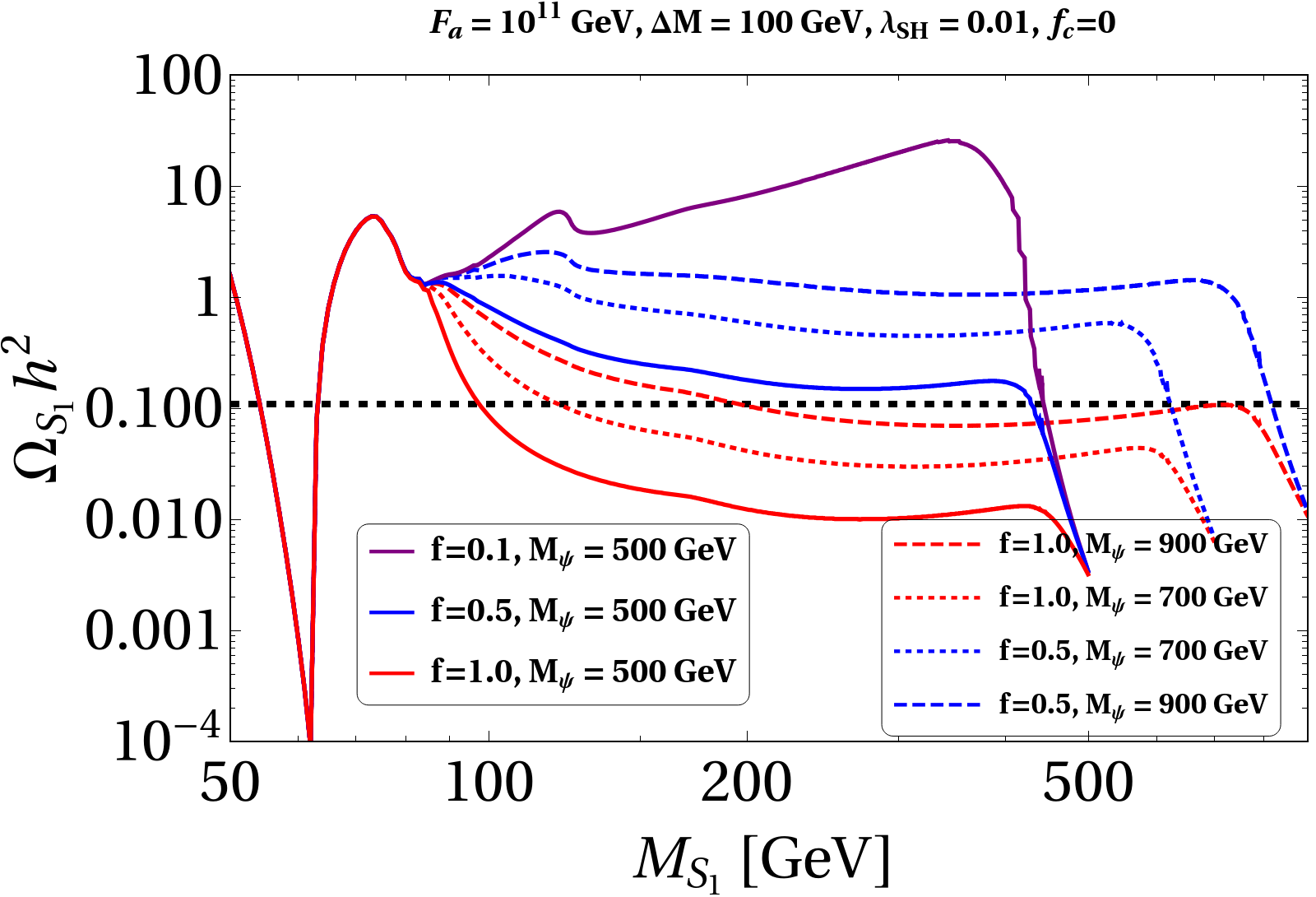
Figure 1: Variations of the scalar DM relic density with its mass ($M_{S_{1}}$) for different values of $f$ and $M_{\Psi}$ are shown. Here, we fix $F_{a}=10^{11}~{}\text{GeV},~{}\lambda_{SH}=0.01$, $f_{c}=0$, and $\Delta M=100$ GeV. The Black dashed line corresponds to $0.120-\Omega_{a}h^{2}$.

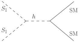
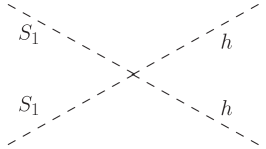
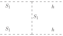
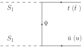
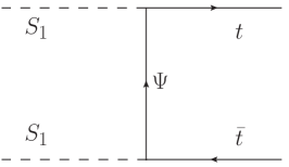
Figure 9: Feynman diagrams of scalar dark matter annihilation into Standard Model particles are presented.

To estimate the component of relic density offered by scalar DM, we solve the Boltzmann equation using micrOMEGAs -v5 Belanger:2018ccd . We first construct our model in Feynrules Alloul:2013bka . The variation of the scalar DM relic density with its mass is displayed in Figure 1 while we fix $F_{a}=10^{11}~{}\text{GeV},~{}\lambda_{SH}=0.01$, $f_{c}=0$, and $\Delta M=100$ GeV. We present three solid lines for three distinct values of democratic coupling $f=0.1,~{}0.5,$ and $1.0$ for the 500 GeV mass of the VLQ. In these variation curves, the first sharp dip ensues due to the Higgs resonance, in which pair of DM annihilate into SM particles through the resonant Higgs boson when $M_{S_{1}}\sim\frac{m_{h}}{2}$, while the second dip occurs when $M_{S_{1}}\sim M_{W}$, in which pair of $S_{1}$ annihilate into a $W$ boson pair through s-channel Higgs-mediated diagram, see Figure 9.

For $f=0.1$ (solid purple line), after the second dip, the relic density increases along with the increase in the DM mass, and a third dip is observed at $M_{S_{1}}=m_{h}$. The pair of $S_{1}$ begin to annihilate into the Higgs bosons via contact interaction, Higgs-mediated s-channel, and $S_{1}$-mediated t-channel diagrams (Figure 9) and produce the third dip. Ultimately, when the mass difference between VLQ and DM becomes smaller, the impact of DM co-annihilation with the VLQ and annihilation of the VLQ pair into gluons becomes apparent, and a final decline in DM relic density is observed. Further increasing $f$ (0.5 with solid blue line and 1.0 with solid red line) reveals that relic density declines just after the second dip due to the significant contribution of $S_{1}S_{1}\rightarrow t\bar{u},~{}\bar{t}u$ annihilation channels via the VLQ-exchange t-channel processes. The correct relic density is achieved for $f=1.0$ when DM mass is around $96$ GeV.

Blue (red) dotted and dashed lines correspond to the same values of $f$ as in solid lines, except with a heavier choice of mediator ${\Psi}$. Because the annihilation cross section decreases as propagator mass increases, and relic density is inversely proportional to the annihilation cross section, the dotted and dashed lines move to higher relic density than the solid line. One clearly follows from these variations that significant parameter space for heavier dark matter masses can open up for different choices of these parameters (over and above the typical Higgs portal). Interestingly, in the case of a pure scalar singlet DM scenario, the DM does not satisfy the correct relic density for $\lambda_{SH}=0.01$. However, the interaction of the DM with the SM top quark in the present model affords many parameter spaces that satisfy the Planck limit.

Direct and indirect detection of DM:

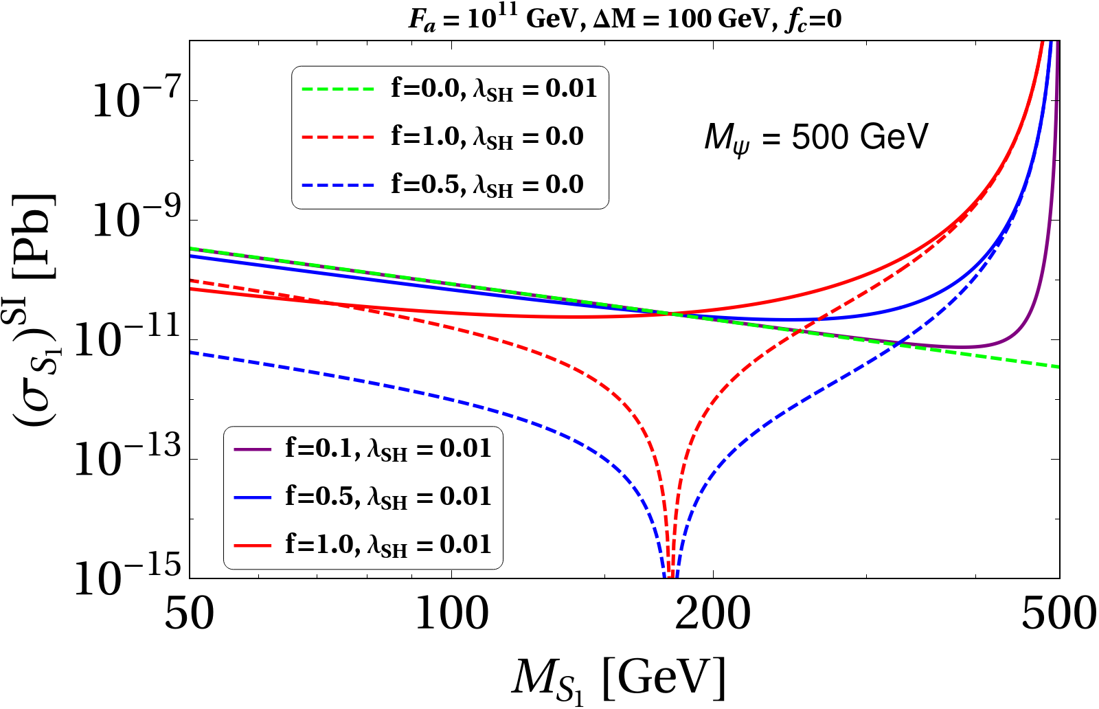
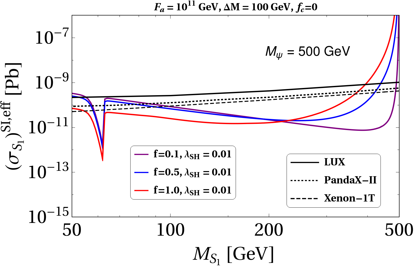
Figure 2: Left panel: Spin-independent cross section of scattering between scalar DM and nucleon as a function of dark matter mass $M_{S_{1}}$. We set $f=0,\lambda_{SH}=0.01$ (green dashed line), and $\lambda_{SH}=0$ for the blue-dashed ($f=0.5$) and red-dashed ($f=1.0$) lines to illustrate the individual contributions. Right panel: Effective spin-independent scattering cross section (Equation 15) vs dark matter mass. All of the plots on the left and right are for $M_{\Psi}=500$ GeV. The solid colours purple, blue, and red in both panels stand for $f=0.1,~{}0.5,$ and $1.0$, respectively, and $\lambda_{SH}=0.01$ for all solid lines.

WIMPs may also scatter off nuclei, depositing energy that can be detected by detectors like LUX Akerib:2016vxi , PandaX-II Tan:2016zwf ; Cui:2017nnn , and XEXON1T Aprile:2018dbl . These experiments can set strong constraints on the scattering cross section and DM mass. All Direct detection channels and the square amplitude of these diagrams are shown in Appendix A. For demonstration purposes, we present a spin-independent direct detection cross section of $S_{1}$ with its mass shown in the left panel of Figure 2. All solid lines correspond to $\lambda_{SH}=0.01$ but for different values of $f=$ 0.1 (solid purple), 0.5 (solid blue), and 1.0 (solid red). Because $f$ and $\lambda_{SH}$ are both non-zero, the Higgs-mediated and VLQ-mediated channels and their interference diagrams contribute. It is instructive to note how individual channel contributes. One can first set $f=0,~{}\lambda_{SH}=0.01$ (dashed green line) so only the Higgs-mediated channel contributes. Subsequently, setting $\lambda_{SH}=0$ for two choices of $f=1.0~{}(0.5)$ in the dashed-red (blue) line demonstrates the contribution from pure VLQ-mediated s and t-channels and their interference diagram. The Higgs-mediated diagram does not contribute here.

The amplitude square of the Higgs-mediated diagram does not rely on the mass of $S_{1}$ (Equation 22); nevertheless, the cross section of the dashed green line decreases with the DM mass, which comes from the phase space part of the integral. We see dashed red and blue lines strongly depend on the $M_{S_{1}}$ since the amplitude square of the VLQ mediated s and t- channels and their interference explicitly depends on $M_{S_{1}}$ (see Equations 18- 21), and the cross section is minimum when $M_{S_{1}}=\dfrac{M_{\Psi}}{2\sqrt{2}}$. When comparing dashed-green (only Higgs-mediated channel contributes), dashed-red (only VLQ-mediated channels contribute), and solid-red (total cross section) lines, one can witness a substantial negative (positive) interference between Higgs and VLQ-mediated diagrams when $M_{S_{1}}<\dfrac{M_{\Psi}}{2\sqrt{2}}$ ($M_{S_{1}}>\dfrac{M_{\Psi}}{2\sqrt{2}}$). Finally, when DM mass is large, we see a sharp rise because of the on-shell production of VLQ (Figure 10a).

In a two-component DM scenario, the direct detection cross section of the scalar DM should be rescaled as

$$\sigma_{S_{1}}^{\text{SI,\text{eff}}}=\Bigl{(}\frac{\Omega_{S_{1}}h^{2}}{\Omega_{\text{T}}h^{2}}\Bigr{)}~{}\sigma_{S_{1}}^{\text{SI}},$$ (15)

where $\Omega_{\text{T}}h^{2}$ is given in Equation 9. The spin-independent effective direct detection cross section for three distinct values of $f=0.1,~{}0.5,$ and $1.0$ are presented in the right panel of Figure 2 (same as solid lines in the left panel). The black lines show the experimental upper bounds. A dip around $M_{S_{1}}\sim\frac{m_{h}}{2}$ is found because of rescaling, as given in Equation 15. Here, one notices that the DD experiments disallow the region with a considerable mass difference between the VLQ and DM for significantly large $f$ values. For example, the regions when $M_{S_{1}}>390$ GeV for $M_{\Psi}=500$ GeV and $f=1$ (solid red line) are disallowed by DD. Additionally, Figures 1 and 2, for $f=1$, suggest that the parameter spaces that offer correct relic density are likewise allowed from the DD.

WIMPs may self-annihilate, emitting a significant amount of gamma and cosmic rays while looking at the dense DM regions at the galactic centre. Indirect detection experiments like PAMELA Kohri:2009yn , Fermi-LAT Eiteneuer:2017hoh , MAGIC Ahnen:2016qkx etc. can constrain model parameter spaces substantially. Because this is a two-component DM scenario, the scalar DM’s indirect detection cross section should also be rescaled as,

$$\sigma^{ID}_{S_{1},\text{eff}}=\Bigl{(}\frac{\Omega_{S_{1}}h^{2}}{\Omega_{\text{T}}h^{2}}\Bigr{)}^{2}~{}\sigma^{ID}_{S_{1}}~{}.$$ (16)

We note that most indirect detection experiments enable our model because the necessity for the axion keeps $S_{1}$ under abundance, which lowers the indirect detection constraints since it depends on the fractional scalar DM relic density squared. For very small $\Delta M$ $=(M_{S_{2}}-M_{S_{1}}$), $S_{1}$ and $S_{2}$ are nearly degenerate and can open an additional channel where $S_{1}$ and $S_{2}$ co-annihilate into top anti-top pair via VLQ and contribute to the indirect detection cross section, which may be disallowed by antiproton cosmic ray data Colucci:2018vxz , so we set $\Delta M=100$ GeV throughout our analysis, ensuring that no co-annihilation channel exists.

Parameter scan and benchmark points:

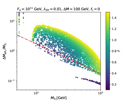
Figure 3: On the $\frac{\Delta M_{\Psi S_{1}}}{M_{S_{1}}}-~{}M_{S_{1}}$ plane, the parameter spaces that satisfy the measured DM abundance, permitted by the direct search experiments, and comply with other restrictions as stated in the text are displayed. The color coding is done with respect to $f$, with $f$ varying from 0.1 to 1.5. Here, we fix $F_{a}=10^{11}~{}\text{GeV},~{}\lambda_{SH}=0.01,~{}\Delta M=100$ GeV, and $f_{c}=0$.

	$M_{S_{1}}$	$\Delta M_{\Psi S_{1}}$	$\Delta M$	$f$	$\Omega_{S_{1}}h^{2}$	$\sigma^{SI}_{S_{1},eff}$	Processes
	(GeV)	(GeV)	(GeV)			(pb)	(percentage)	BR($\Psi\rightarrow tS_{1,2}$)
BP1	332	500	100	0.83	0.109	$7.98\times 10^{-12}$	$S_{1}S_{1}\rightarrow t\bar{u},\bar{t}u~{}(60\%)$	0.4907
							$S_{1}S_{1}\rightarrow t\bar{t}~{}(40\%)$
BP2	402	407	100	0.82	0.109	$7.65\times 10^{-12}$	$S_{1}S_{1}\rightarrow t\bar{u},\bar{t}u~{}(56\%)$	0.4875
							$S_{1}S_{1}\rightarrow t\bar{t}~{}(44\%)$
BP3	450	300	100	0.79	0.107	$1.14\times 10^{-11}$	$S_{1}S_{1}\rightarrow t\bar{u},\bar{t}u~{}(54\%)$	0.435
							$S_{1}S_{1}\rightarrow t\bar{t}~{}(45\%)$

Table 1: A few representative benchmark points (BPs) from the scan plot are presented; these BPs satisfy the correct relic density and are permissible under all constraints. $\Omega_{S_{1}}h^{2}$ and $\sigma^{SI}_{S_{1},eff}$ (Equation 15) are the relic density and the effective direct detection cross section of the scalar DM, $S_{1}$, respectively. $\Delta M_{\Psi S_{1}}=M_{\Psi}-M_{S_{1}}$ and $\Delta M=M_{S_{2}}-M_{S_{1}}$. Other parameters are $F_{a}=10^{11}~{}\text{GeV},~{}\lambda_{SH}=0.01,~{}\text{and}~{}f_{c}=0$. The second last column shows the different processes that contribute to the relic density with the percentage contributions in the bracket. The branching fraction of VLQ decays into the top quark associated with the scalar is shown in the last column.

	$\sigma_{S_{1}}^{\text{ID}}$	$S_{1}S_{1}\rightarrow t\bar{u},\bar{t}u$	$S_{1}S_{1}\rightarrow t\bar{t}$	$\sigma^{ID}_{S_{1},\text{eff}}$ (in $t\bar{t}$)	$\sigma^{ID}_{exp}$ (in $t\bar{t}$)
BP	($cm^{3}/s$)	(in $\%$)	(in $\%$)	($cm^{3}/s$)	($cm^{3}/s$)
BP1	$2.30\times 10^{-26}$	59.8	40.0	$7.59\times 10^{-27}$	$2.37\times 10^{-26}$
BP2	$2.36\times 10^{-26}$	56.0	43.7	$8.51\times 10^{-27}$	$2.54\times 10^{-26}$
BP3	$2.43\times 10^{-26}$	54.4	45.4	$8.77\times 10^{-27}$	$2.60\times 10^{-26}$

Table 2: Total indirect detection cross section, $\sigma_{S_{1}}^{\text{ID}}$ and the percentage of the different processes that contribute to indirect detection are presented in the third and fourth columns. Effective indirect detection cross section in the $t\bar{t}$ final state for different benchmark points is shown in the fifth column, which is defined as $(\text{\% contribution in}~{}t\bar{t}~{}\text{final state})\times\sigma^{ID}_{S_{1},\text{eff}}$, where $\sigma^{ID}_{S_{1},\text{eff}}$ is given in Equation 16. The last column is the experimental upper bound in the $t\bar{t}$ final state  Colucci:2018vxz .

To demonstrate the relevant parameter space that offers correct relic abundance while being allowed by direct detection and all other constraints as specified in the last section, we identify the three most important parameters, that is, the masses $M_{S_{1}}$, $\Delta M_{\Psi S_{1}}$ and the Yukawa coupling $f$. Figure 3 display such points on the plane of $M_{S_{1}}$ vs $\frac{\Delta M_{\Psi S_{1}}}{M_{S_{1}}}$, while the Yukawa coupling $f$ is colour coded, with $f$ ranging from 0.1 to 1.5. The red dash-dot line corresponds to $\Delta M_{\Psi S_{1}}=m_{t}$. Hence, the upper portions of this line may be investigated at the LHC with top quark on-shell production as VLQ decays into a top quark and invisible DM, while the lower area can be probed with jets $+$ MET as VLQ decays into an $u$-quark associated with DM. Points along two vertical lines at the top left region correspond to the part satisfied by Higgs resonance.

It is enlightening to note that the lower sections of the plot, which correspond to the small mediator mass $M_{\Psi}$, typically generate an increased DD cross section; therefore, those regions are excluded from the DD bounds despite having the correct relic density. Only a few points exist at the lower right corner when $f$ is tiny. Those regions have correct relic density because being nearly degenerate, the VLQ and DM co-annihilate and the pair of VLQ annihilates into gluons. Note that for larger $f$ values, those co-annihilation regions are ruled out by the DD experiments, as we already see in Figure 2 (right panel, red, blue lines). Interestingly, non-perturbative effects like Sommerfeld enhancement and bound state formation can significantly affect relic density in those co-annihilation regions. Further study of this region is beyond the scope of the present discussion. Such points are challenging to probe at the LHC as the DM mass is quite large and VLQ is degenerate to the DM, so the partonic cross section of VLQ production will be small, and VLQ will emit a soft jet that is very difficult to detect.

A few representative benchmark points (BPs) from the scan plot are listed in Table 1, which are allowed from all the constraints and provide correct relic density. The scalar DM relic density, spin-independent DD scattering cross section of $S_{1}$, the percentage contribution of each process to the relic density, and the branching ratio of VLQ decay into the top quark are also given. Table 2 shows the total cross section of indirect detection (ID) and the percentage contribution of the various processes to the indirect detection. The theoretical ID cross section in the final state of $t\bar{t}$ and the experimental upper bound are given in the last two columns, where we find that all of those BPs are well inside the experimental upper bound.

4 Pair production of vector-like quark at NLO+PS accuracy

We implement the model Lagrangian discussed in Equation 3 together with the interaction terms of Equations 5 and 6 in FeynRules Alloul:2013bka and employ the NLOCT Degrande:2014vpa package to generate UV and $R_{2}$ counterterms of the virtual contribution in NLO UFO model that we finally use under the MadGraph5_aMC@NLO Alwall:2014hca environment. Inside this, the real corrections are performed using the FKS subtraction method Frixione:1995ms ; Frixione:1997np , whereas the OPP technique Ossola:2006us takes care of the virtual contributions. Showering of the events is done using Pythia8 Sjostrand:2001yu ; Sjostrand:2014zea . For leading order (LO) and next-to-leading order (NLO) event generation, we use NN23LO and NN23NLO PDF sets, respectively.

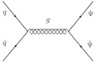
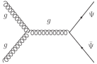
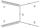
(a) $\mathcal{M}_{\text{LO}}^{a}=\mathcal{O}(\alpha_{S})$

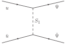
(b) $\mathcal{M}_{\text{LO}}^{b}=\mathcal{O}(f^{2})$

Figure 4: The Feynman diagrams for the pair production of VLQ at Leading order. The three diagrams at the top only contain QCD coupling, whereas the two diagrams at the bottom only have pure BSM couplings ($f$), and their interference terms are also present. The LO cross section, $\sigma_{\text{LO}}=\mathcal{O}(\alpha_{S}^{2})+\mathcal{O}(f^{4})+\mathcal{O}(f^{2}\alpha_{S})$.

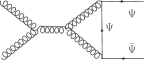
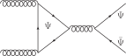
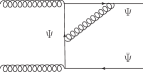
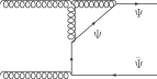
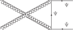
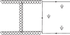
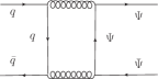
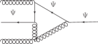
Figure 5: Representative Feynman diagrams for the pair production of VLQ at NLO-QCD for the processes where the tree-level diagrams only have QCD coupling (Figure 4a). $\sigma_{\text{NLO}}^{a}\propto\mathcal{M}_{V}^{\dagger}\mathcal{M}_{\text{LO}}^{a}=\mathcal{O}(\alpha_{S}^{3})$.

All the tree-level diagrams in the pair production of VLQ at the LHC are shown in Figure 4, where the top three Feynman diagrams depend only on the QCD coupling, whereas the bottom two channels depend only on the BSM Yukawa coupling, $f$. The LO cross section has the order $\sigma_{\text{LO}}=\mathcal{O}(\alpha_{S}^{2})+\mathcal{O}(f^{4})+\mathcal{O}(f^{2}\alpha_{S})$, where the interference between the top and bottom channels provides the $\mathcal{O}(f^{2}\alpha_{S})$ term.

	$\sigma(pp\rightarrow\Psi\bar{\Psi})$ (fb)	$\sigma(pp\rightarrow\Psi\bar{\Psi})$ (fb) for
BP	LO	leading production processes at LO and NLO
	$\sigma_{\text{LO}}=\mathcal{O}(\alpha_{S}^{2})+\mathcal{O}(f^{4})+\mathcal{O}(f^{2}\alpha_{S})$	LO, $~{}~{}\mathcal{O}(\alpha_{S}^{2})$	NLO, $~{}~{}\mathcal{O}(\alpha_{S}^{3})$	K-fac
BP1	$96.39^{+31.5\%}_{-22.5\%}$	$105.8^{+31.3\%}_{-22.2\%}$	$138.5^{+9.6\%}_{-11.3\%}$	1.31
BP2	$114.0^{+31.9\%}_{-22.5\%}$	$125.7^{+31.4\%}_{-22.4\%}$	$162.1^{+10.1\%}_{-11.5\%}$	1.29
BP3	$181.5^{+32.1\%}_{-22.7\%}$	$201.6^{+31.3\%}_{-22.3\%}$	$257.3^{+9.8\%}_{-11.4\%}$	1.28

Table 3: Total leading-order cross section, including QCD and BSM coupling, and their interference in the pair production of VLQ at 14 TeV LHC before their decay is given in the left panel. Right panel: Leading contribution of the tree-level VLQ pair production process ($\mathcal{O}(\alpha_{S}^{2})$) and its next-to-leading order cross section, along with the integrated K-factor, are given. The superscript and subscript denote the scale uncertainties (in percentage) of the total cross section. Five massless quark flavors are used for computation.

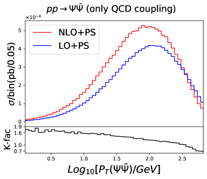
(a)

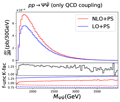
(b)

Figure 6: (a) Distribution of $\log_{10}[P_{T}(\Psi\bar{\Psi})/GeV]$ at LO+PS and NLO+PS, and the differential K-factor for VLQ pair production at the LHC. (b) The distribution of invariant mass of the VLQ pair is shown in the upper panel, and the differential K-factor and the scale uncertainties are shown in the middle and bottom panels, respectively. The plots correspond to BP1, and LO consists only of QCD coupling.

At LO, we keep all contributions coming from pure QCD ($\mathcal{O}(\alpha_{S}^{2})$), which gives the leading contribution, and from BSM coupling and their interference in the pair production of VLQ at the LHC. We do one-loop QCD correction of the processes that have only strong couplings at the tree level; therefore, NLO corrections have order $\mathcal{O}(\alpha_{S}^{3})$. Few representative Feynman diagrams at NLO-QCD are shown in Figure 5. The total LO cross section is given in the left panel of Table 3. The leading contribution of the VLQ pair production at the tree level and its next-to-leading order cross section, along with the integrated K-factor, are given in the right panel of Table 3. The K-factor is defined as the ratio of NLO to LO cross section. We find a significant enhancement of about $30\%$ in the NLO-QCD cross section over LO. Table 3 shows that the interference term has a non-negligible negative contribution to the total LO cross section.

We designate the partonic centre-of-mass energy of the event as the central choice for both the factorization and renormalization scales. To compute the scale variance, we vary both the factorization and renormalization scales from a factor of two to half of this central scale, resulting in nine different data sets. The superscripts and subscripts in the tables indicate the envelopes of the nine data sets, although all of the cross sections shown in Table 3 correspond to the central scale.

LO+PS and NLO+PS distributions of $\log_{10}[P_{T}(\Psi\bar{\Psi})/GeV]$ (upper panel) and the differential K-factor (lower panel) are given in Figure 6a. $P_{T}(\Psi\bar{\Psi})$ is the transverse momentum of the VLQ pair. For $\log_{10}[P_{T}(\Psi\bar{\Psi})/GeV]<2.6$, the left plot shows that K-factor is more than 1, but for $\log_{10}[P_{T}(\Psi\bar{\Psi})/GeV]>2.6$, the K-factor is less than 1, indicating that the NLO cross section is less than the LO cross section. The differential K-factor is not flat everywhere. It is almost flat at the lower values and then starts to go down, so scaling the LO events by a constant K-factor would not give accurate results.

The invariant mass distribution of the VLQ pair is shown on the top panels of Figure 6b for BP1. The differential K-factor is shown in the middle panel. Invariant mass distribution peaks around 1800 GeV, and the differential K-factor is almost flat around the peak. The bottom panel shows the envelope of the factorization and renormalization scale uncertainties. The red solid and dashed lines show the width of the scale uncertainty for NLO+PS, while the blue solid and dashed lines show the LO+PS scale uncertainties. We can see that both LO+PS and NLO+PS results are stable, but the NLO+PS result has much-reduced scale uncertainty. Although these are figurative findings because $\Psi$ decay is not taken into account, they demonstrate the need to do $\mathcal{O}(\alpha_{s})$ corrections on the pair production channels to predict the production rate and lower scale uncertainty.

5 Multivariate Analysis (MVA)

For completeness, we further carried out the collider analysis on this model using the $t\bar{t}+\text{MET}$ final state, as in our earlier study Ghosh:2022rta . The reference includes all the backgrounds and kinematic cuts. However, here, we use the NLO event to generate the signal. Moreover, the previous analysis assumed the $\text{BR}(\Psi\rightarrow tS_{1,2})=1.0$, based on the top-philic coupling, which is invalid for a democratic coupling with other generations. Hence, based on calculated $\text{BR}(\Psi\rightarrow tS_{1,2})<0.5$ (Table 1) for all the BPs when the pair of $\Psi$ decay into the top quark, the cross section is reduced by a factor of at least 0.25 than the previous. In contrast to the prior assessment, the QCD correction significantly increases the overall cross section, and the Yukawa coupling considerably impacts the partonic cross section.

The signal topology is given by ,

$$pp\rightarrow\Psi\bar{\Psi}\hskip 2.84526pt\text{[QCD]}\rightarrow(t\hskip 2.84526ptS_{1,2})(\bar{t}\hskip 2.84526ptS_{1,2})\hskip 2.84526ptj\Rightarrow 2J_{t}+\not{E}_{T}+X$$ (17)

	Signal (BP1)	$Z$+jets	$W$+jets	$t\bar{t}$+jets	$tW$+jets	$WZ$+j	$WW$+j	$ZZ$+j	$t\bar{t}~{}V$	tot BG
	(fb)	(fb)	(fb)	(fb)	(fb)	(fb)	(fb)	(fb)	(fb)	(fb)
C1	5.99	2517.99	1366.91	690.65	366.91	93.53	25.90	11.51	8.34	5081.74
	[$100\%$]	[$100\%$]	[$100\%$]	[$100\%$]	[$100\%$]	[$100\%$]	[$100\%$]	[$100\%$]	[$100\%$]	[$100\%$]
C2	5.49	1640.29	762.59	302.16	152.52	58.35	11.51	6.973	6.17	2940.56
	[$91.65\%$]	[$65.14\%$]	[$55.79\%$]	[$43.75\%$]	[$41.57\%$]	[$62.39\%$]	[$44.44\%$]	[$60.58\%$]	[$73.98\%$]	[$57.87\%$]
C3	4.58	241.73	117.99	230.94	114.39	10.79	2.45	1.92	5.11	725.32
	[$76.46\%$]	[$9.60\%$]	[$8.63\%$]	[$33.44\%$]	[$31.18\%$]	[$11.54\%$]	[$9.46\%$]	[$16.69\%$]	[$61.27\%$]	[$14.27\%$]
C4	2.23	25.38	17.33	64.23	27.45	1.24	0.33	0.2	2.30	138.46
	[$37.23\%$]	[$1.01\%$]	[$1.27\%$]	[$9.30\%$]	[$7.48\%$]	[$1.33\%$]	[$1.27\%$]	[$1.74\%$]	[$28.13\%$]	[$2.72\%$]

Table 4: After applying various kinematic event selection cuts, signal and background events (in fb) indicate the efficiency for each set of cuts to reduce the backgrounds. The kinematic cuts (C1-C4) are described in the text. After applying the C4 cut, the remaining events are passed for the multivariate analysis.

	$\not{E}_{T}$	$\Delta\phi(J_{1},\not{E}_{T})$	$\Delta R(J_{0},J_{1})$	$\tau_{32}(J_{1})$	$\tau_{32}(J_{0})$	$\Delta\phi(J_{0},\not{E}_{T})$	$\text{M}_{\text{eff}}$	$M(J_{1})$	$M(J_{0})$	$\tau_{31}(J_{0})$	$\tau_{31}(J_{1})$
BP1	31.29	20.19	17.82	8.61	8.49	8.38	3.29	2.10	1.48	1.10	0.9
BP2	19.39	16.74	17.39	6.75	6.99	8.04	2.26	0.67	0.72	1.11	0.73
BP3	9.25	11.30	12.11	6.52	5.74	6.55	1.29	0.95	0.38	0.52	0.72

Table 5: Method unspecific relative separation power of different kinematic variables in separating the signal and background classes.

The expected number of signal (BP1) and background events (in fb, expected event numbers are obtained by multiplying them with the luminosity) is listed as cut flow, along with the cut efficiencies, after each set of event selection criteria is shown in Table 4. In preselection cut (C1) we demand at least two fatjets of radius $R=1.5$, each with a transverse momentum $P_{T}(J_{0}),P_{T}(J_{1})>200$ GeV, missing transverse momentum $\not{E}_{T}>100$ GeV, a lepton-veto, and $|\Delta\Phi(J_{0,1},\not{E}_{T})|>0.2$ (to minimize jet mismeasurement contribution to $\not{E}_{T}$). The other cuts are: (C2) $\not{E}_{T}>150$ GeV, (C3) a b-tag within the leading or subleading fatjet, and (C4) pruned mass of the two leading jets $M_{J_{0}},M_{J_{1}}>120$ GeV. After applying the preselection cut (C1), we find $V$+jets ($V=Z,W$) are the principal background while $t\bar{t}$+jets is the subdominant background. However, after a b-tag within $J_{0}$ or $J_{1}$ and demanding large fatjet masses, we found $t\bar{t}$+jets becomes the primary background, while $V$+jets are the subdominant. Applying all those cuts, we still retain a substantial number of signal events while the background reduces significantly.

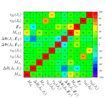
(a)

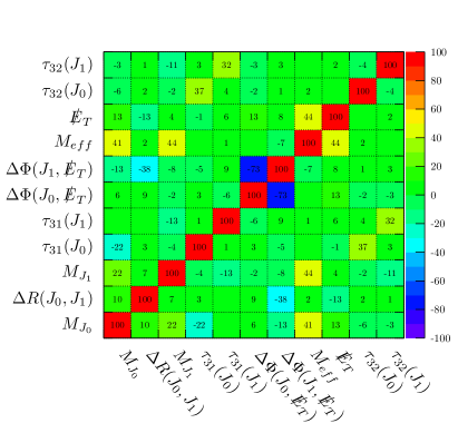
(b)

Figure 7: Coefficients of linear correlation (in percentage) between various kinematical variables for the signal (BP1, left panel) and background (right panel) are presented. Missing entries have an insignificant correlation of less than one. Two variables are correlated or anti-correlated based on positive and negative coefficients.

All the signal and background processes are passed through all these event selection criteria up to C4 before passing events to MVA. We create two separate signal and background classes. The combined background is the weighted combination of all the different background processes. Each signal and background class is randomly divided into $50\%$ for training and the rest $50\%$ for testing. We use boosted decision tree (BDT) algorithm and choose a set of kinematic variables from a wider collection of variables for MVA. The variables with high relative importance distinguishing the signal class from the background class are preferable. Table 5 lists the relative importance of the various kinematic variables involved in the MVA. The left (signal) and right (background) tables of Figure 7 show the linear correlation coefficients among the variables employed in MVA for BP1.

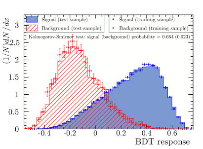
(a)

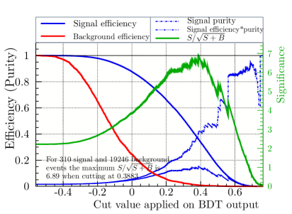
(b)

Figure 8: The left panel shows the normalized distribution of the BDT output for training and testing samples of both signal and background. The statistical significance of the signal with the cut applied to the BDT output is shown in the right panel, along with signal and background efficiency.

	$N_{S}^{bc}$ (fb)	BD$T_{opt}$	$N_{S}$ (fb)	$N_{B}$ (fb)	$\frac{N_{S}}{\sqrt{N_{S}+N_{B}}}$ for 139 $\text{fb}^{-1}$	$\frac{N_{S}}{N_{B}}$
BP1	2.23	0.3883	0.8012	1.0783	6.89	0.743
BP2	2.53	0.2582	1.2207	6.1302	5.31	0.199
BP3	1.67	0.2961	0.4252	2.3529	3.0	0.180
$N_{SM}$	138.46

Table 6: The table shows the efficacy of the current search in terms of statistical significance for various benchmarks. $N_{S}^{bc}$ and $N_{SM}$ are the total numbers of signal and background events before performing MVA (see Table 4), while $N_{S}$ and $N_{B}$, respectively, provide those following BDT analysis. BD$T_{opt}$ is the optimal BDT cut. The second-to-last column provides the statistical significance of the signal for 139 $\text{fb}^{-1}$ luminosity.

Reference Ghosh:2022rta provides the normalized distributions of all background processes after performing all event selections up to C4. We avoid demonstrating these distributions since the shapes are qualitatively similar for physics understanding. The normalized distribution of the BDT response for test and train samples of both signal (BP1) and background classes is plotted on the left side of Figure 8. We find signal and background are well separated. With the cut applied to the BDT output, the signal and background efficiency, as well as the statistical significance ($\frac{N_{S}}{\sqrt{N_{S}+N_{B}}}$) for 139 $\text{fb}^{-1}$ data, are presented in the right plot of Figure 8. Before applying any cuts to the BDT output, Table 6 shows the number of signals ($N_{S}^{bc}$) and background ($N_{SM}$) events for various BPs. It also shows the expected number of signal events ($N_{S}$) and background events ($N_{B}$) that remain after applying an optimal cut (BD$T_{opt}$) to the BDT output. The last two columns show the statistical significance of the signal at 139 $\text{fb}^{-1}$ luminosity and the signal-to-background ratio. We optimize each of the three BPs separately.

Table 6 shows that the statistical significance of BP3 is lower than that of the other two benchmark points even though it has the most significant partonic cross section of VLQ pair production since the mass of the VLQ is the smallest for BP3. This is attributed to a smaller mass difference between VLQ and DM than the other two BPs, which results in a relatively less boosted top quark and a smaller signal efficiency. Table 6 also demonstrate that a significant parameter space of this model can be explored with more than $5\sigma$ significance using the 139 $\text{fb}^{-1}$ data at the 14 TeV LHC.

6 Conclusions

We explore a complex scalar extended KSVZ axion framework, where the scalar is singlet under SM gauge groups but only has the Peccei-Quinn charge. This model has the capability to solve two of the most outstanding problems of SM, that is, the strong-CP problem and a natural candidate for dark matter in the form of QCD axion having a lifetime comparable to the age of the Universe. Axion can satisfy the correct dark matter relic density, measured by the Planck collaboration, but at the expense of fine-tuning the corresponding breaking scale. The residual $\mathbb{Z}_{2}$ symmetry in this model ensures that the lightest component of scalar extension is stable and thus plays the role of a second dark matter, removing the need for any such fine-tuning.

KSVZ axion framework also provides a rich phenomenology by introducing a vector-like quark which can be explored at a hadron collider like LHC. In the extended scenario, VLQ interacts with the scalar (DM) candidate and SM quarks (up or down) based on its hypercharge. Hence the VLQ now plays a critical role in dark matter phenomenology because it opens up new annihilation and coannihilation channels.

Here, we explore the possibility of democratic Yukawa interaction of the vector-like quark with all up-type quarks and scalar dark matter candidate. One must find the allowed parameter spaces that provide the correct relic density and agree with other experimental observations such as direct detection (DD), collider data, etc. It is found that the flavour constraint strongly disfavours this democratic option, which requires either one or both lighter flavour couplings ($f_{u},f_{c}$) needs to be tiny. For simplicity, we consider $f_{c}=0$ while keeping the other two democratic. It is interesting to note that the allowed parameter space can neither support arbitrarily large coupling $f(=f_{u}=f_{t})$ from direct detection nor the too-small value of it to obtain the correct relic density. Therefore, their interplay remains vital for selecting the available parameter spaces.

We employ next-to-leading order NLO-QCD correction for VLQ pair production to study a unique search strategy at the LHC, generating a pair of boosted tops with sizeable missing transverse momentum. Boosted top-like fatjets generated from the hadronic decay of top quark still carry different characteristics of it, which are primarily captured in a dedicated jet analysis and different substructure variables. Multivariate analysis with these variables and attributes of event topology is demonstrated to establish a strong ability to explore a significant parameter space of this model at the 14 TeV LHC.

Appendix A Appendix

Direct detection channels:

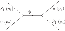
(a) $\mathcal{M}_{1}$

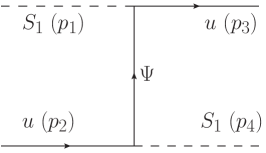
(b) $\mathcal{M}_{2}$

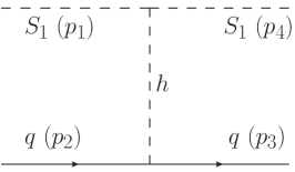
(c) $\mathcal{M}_{3}$

Figure 10: Scattering diagrams between scalar dark matter and the nucleon.

Three different channels (Figure 10) are possible at the tree level for the scattering process $S_{1}(p_{1})~{}u(p_{2})\rightarrow S_{1}(p_{4})~{}u(p_{3})$, VLQ-mediated s-channel, VLQ-mediated t-channel, and Higgs-mediated t-channel diagrams. The total cross section comprises the amplitude square of the individual channels and the interference between different diagrams. The interference with different diagrams and the amplitude square of the individual diagrams are provided below.
Amplitude square of VLQ-mediated s-channel diagram:

$$\mathcal{M}_{1}^{\dagger}\mathcal{M}_{1}=\dfrac{f^{4}}{4}~{}\dfrac{\mathcal{N}+m_{u}^{2}~{}(p_{1}.p_{2}+p_{1}.p_{3})}{[(p_{1}+p_{2})^{2}-M_{\Psi}^{2}~{}]^{2}}$$ (18)

Amplitude square of VLQ-mediated t-channel diagram:

$$\mathcal{M}_{2}^{\dagger}\mathcal{M}_{2}=\dfrac{f^{4}}{4}~{}\dfrac{\mathcal{N}-m_{u}^{2}~{}(p_{1}.p_{2}+p_{1}.p_{3})}{[(p_{3}-p_{1})^{2}-M_{\Psi}^{2}~{}]^{2}}$$ (19)

Interference between VLQ-mediated s and t-channel diagrams:

$$2\mathcal{M}_{1}^{\dagger}\mathcal{M}_{2}=-2\times\dfrac{f^{4}}{4}~{}\dfrac{\mathcal{N}+m_{u}^{2}~{}(-p_{1}.p_{2}+p_{1}.p_{3})}{[(p_{1}+p_{2})^{2}-M_{\Psi}^{2}~{}][(p_{3}-p_{1})^{2}-M_{\Psi}^{2}~{}]}$$ (20)

Where $p_{2}^{2}=p_{3}^{2}=m_{u}^{2}$, $p_{1}^{2}=p_{4}^{2}=M_{S_{1}}^{2}$, and $\mathcal{N}$ is given below.

$$\mathcal{N}=2(p_{1}.p_{3})(p_{1}.p_{2})+M_{S_{1}}^{2}~{}(p_{1}.p_{3}-p_{1}.p_{2}-m_{u}^{2})+m_{u}^{4}$$ (21)

Amplitude square of Higgs-mediated t-channel diagram:

$$\mathcal{M}_{3}^{\dagger}\mathcal{M}_{3}=2m_{q}^{2}\lambda_{SH}^{2}\cos^{2}\theta~{}\dfrac{p_{1}.p_{3}-p_{1}.p_{2}-2m_{u}^{2}}{[(p_{4}-p_{1})^{2}-M_{h}^{2}~{}]^{2}}$$ (22)

Interference between VLQ-mediated s-channel and Higgs-mediated t-channel diagrams:

$$2\mathcal{M}_{1}^{\dagger}\mathcal{M}_{3}=2m_{u}^{2}\lambda_{SH}\cos\theta f^{2}~{}\dfrac{p_{1}.p_{2}+m_{u}^{2}}{[(p_{1}+p_{2})^{2}-M_{\Psi}^{2}~{}][(p_{4}-p_{1})^{2}-M_{h}^{2}~{}]}$$ (23)

Interference between VLQ-mediated t-channel and Higgs-mediated t-channel diagrams:

$$2\mathcal{M}_{2}^{\dagger}\mathcal{M}_{3}=-~{}2m_{u}^{2}\lambda_{SH}\cos\theta f^{2}~{}\dfrac{p_{1}.p_{3}-m_{u}^{2}}{[(p_{3}-p_{1})^{2}-M_{\Psi}^{2}~{}][(p_{4}-p_{1})^{2}-M_{h}^{2}~{}]}$$ (24)

References

- (1) H.-Y. Cheng, The Strong CP Problem Revisited, Phys. Rept. 158 (1988) 1.
- (2) V. Baluni, CP Violating Effects in QCD, Phys. Rev. D 19 (1979) 2227.
- (3) M. Dine, TASI lectures on the strong CP problem, in Theoretical Advanced Study Institute in Elementary Particle Physics (TASI 2000): Flavor Physics for the Millennium, pp. 349–369, 6, 2000, hep-ph/0011376.
- (4) Y. Sofue and V. Rubin, Rotation curves of spiral galaxies, Ann. Rev. Astron. Astrophys. 39 (2001) 137 [astro-ph/0010594].
- (5) D. Clowe, M. Bradac, A. H. Gonzalez, M. Markevitch, S. W. Randall, C. Jones et al., A direct empirical proof of the existence of dark matter, Astrophys. J. 648 (2006) L109 [astro-ph/0608407].
- (6) A. Riotto and M. Trodden, Recent progress in baryogenesis, Ann. Rev. Nucl. Part. Sci. 49 (1999) 35 [hep-ph/9901362].
- (7) M. Dine and A. Kusenko, The Origin of the matter - antimatter asymmetry, Rev. Mod. Phys. 76 (2003) 1 [hep-ph/0303065].
- (8) Super-Kamiokande collaboration, Evidence for oscillation of atmospheric neutrinos, Phys. Rev. Lett. 81 (1998) 1562 [hep-ex/9807003].
- (9) SNO collaboration, Direct evidence for neutrino flavor transformation from neutral current interactions in the Sudbury Neutrino Observatory, Phys. Rev. Lett. 89 (2002) 011301 [nucl-ex/0204008].
- (10) K2K collaboration, Indications of neutrino oscillation in a 250 km long baseline experiment, Phys. Rev. Lett. 90 (2003) 041801 [hep-ex/0212007].
- (11) C. Abel, S. Afach, N. J. Ayres, C. A. Baker, G. Ban, G. Bison et al., Measurement of the permanent electric dipole moment of the neutron, Phys. Rev. Lett. 124 (2020) 081803.
- (12) R. D. Peccei and H. R. Quinn, CP Conservation in the Presence of Instantons, Phys. Rev. Lett. 38 (1977) 1440.
- (13) R. D. Peccei and H. R. Quinn, Constraints Imposed by CP Conservation in the Presence of Instantons, Phys. Rev. D 16 (1977) 1791.
- (14) J. E. Kim, Weak Interaction Singlet and Strong CP Invariance, Phys. Rev. Lett. 43 (1979) 103.
- (15) M. A. Shifman, A. I. Vainshtein and V. I. Zakharov, Can Confinement Ensure Natural CP Invariance of Strong Interactions?, Nucl. Phys. B 166 (1980) 493.
- (16) Planck collaboration, Planck 2018 results. X. Constraints on inflation, 1807.06211.
- (17) A. Ghosh, P. Konar and R. Roshan, Top-philic dark matter in a hybrid KSVZ axion framework, JHEP 12 (2022) 167 [2207.00487].
- (18) Planck collaboration, Planck 2018 results. VI. Cosmological parameters, 1807.06209.
- (19) B. Dasgupta, E. Ma and K. Tsumura, Weakly interacting massive particle dark matter and radiative neutrino mass from Peccei-Quinn symmetry, Phys. Rev. D 89 (2014) 041702 [1308.4138].
- (20) S. Chatterjee, A. Das, T. Samui and M. Sen, Mixed WIMP-axion dark matter, Phys. Rev. D 100 (2019) 115050 [1810.09471].
- (21) K. J. Bae, J.-H. Huh and J. E. Kim, Update of axion CDM energy, JCAP 09 (2008) 005 [0806.0497].
- (22) G. Raffelt and D. Seckel, Bounds on Exotic Particle Interactions from SN 1987a, Phys. Rev. Lett. 60 (1988) 1793.
- (23) S. Profumo, L. Giani and O. F. Piattella, An Introduction to Particle Dark Matter, Universe 5 (2019) 213 [1910.05610].
- (24) T. Robens and T. Stefaniak, LHC Benchmark Scenarios for the Real Higgs Singlet Extension of the Standard Model, Eur. Phys. J. C 76 (2016) 268 [1601.07880].
- (25) F. Giacchino, A. Ibarra, L. Lopez Honorez, M. H. G. Tytgat and S. Wild, Signatures from Scalar Dark Matter with a Vector-like Quark Mediator, JCAP 1602 (2016) 002 [1511.04452].
- (26) OPAL collaboration, Search for scalar top and scalar bottom quarks at LEP, Phys. Lett. B 545 (2002) 272 [hep-ex/0209026].
- (27) ATLAS collaboration, Search for squarks and gluinos with the ATLAS detector in final states with jets and missing transverse momentum using 20.3 of = 8 TeV proton-proton collision data, in 2nd Large Hadron Collider Physics Conference, 8, 2014, 1408.5857.
- (28) ATLAS collaboration, Search for a scalar partner of the top quark in the jets plus missing transverse momentum final state at =13 TeV with the ATLAS detector, JHEP 12 (2017) 085 [1709.04183].
- (29) ATLAS collaboration, Search for direct top squark pair production in final states with two leptons in TeV collisions with the ATLAS detector, Eur. Phys. J. C 77 (2017) 898 [1708.03247].
- (30) ATLAS collaboration, Search for supersymmetry in final states with two same-sign or three leptons and jets using 36 fb-1 of TeV collision data with the ATLAS detector, JHEP 09 (2017) 084 [1706.03731].
- (31) CMS collaboration, Search for new phenomena with the variable in the all-hadronic final state produced in proton–proton collisions at TeV, Eur. Phys. J. C 77 (2017) 710 [1705.04650].
- (32) CMS collaboration, Search for direct production of supersymmetric partners of the top quark in the all-jets final state in proton-proton collisions at TeV, JHEP 10 (2017) 005 [1707.03316].
- (33) CMS collaboration, Search for top squark pair production in pp collisions at TeV using single lepton events, JHEP 10 (2017) 019 [1706.04402].
- (34) CMS collaboration, Search for top squarks and dark matter particles in opposite-charge dilepton final states at 13 TeV, Phys. Rev. D 97 (2018) 032009 [1711.00752].
- (35) M. Garny, A. Ibarra, S. Rydbeck and S. Vogl, Majorana Dark Matter with a Coloured Mediator: Collider vs Direct and Indirect Searches, JHEP 06 (2014) 169 [1403.4634].
- (36) O. Gedalia, Y. Grossman, Y. Nir and G. Perez, Lessons from Recent Measurements of D0 - anti-D0 Mixing, Phys. Rev. D 80 (2009) 055024 [0906.1879].
- (37) G. Bélanger, F. Boudjema, A. Goudelis, A. Pukhov and B. Zaldivar, micrOMEGAs5.0 : Freeze-in, Comput. Phys. Commun. 231 (2018) 173 [1801.03509].
- (38) A. Alloul, N. D. Christensen, C. Degrande, C. Duhr and B. Fuks, FeynRules 2.0 - A complete toolbox for tree-level phenomenology, Comput. Phys. Commun. 185 (2014) 2250 [1310.1921].
- (39) LUX collaboration, Results from a search for dark matter in the complete LUX exposure, Phys. Rev. Lett. 118 (2017) 021303 [1608.07648].
- (40) PandaX-II collaboration, Dark Matter Results from First 98.7 Days of Data from the PandaX-II Experiment, Phys. Rev. Lett. 117 (2016) 121303 [1607.07400].
- (41) PandaX-II collaboration, Dark Matter Results From 54-Ton-Day Exposure of PandaX-II Experiment, Phys. Rev. Lett. 119 (2017) 181302 [1708.06917].
- (42) XENON collaboration, Dark Matter Search Results from a One Ton-Year Exposure of XENON1T, Phys. Rev. Lett. 121 (2018) 111302 [1805.12562].
- (43) K. Kohri, A. Mazumdar, N. Sahu and P. Stephens, Probing Unified Origin of Dark Matter and Baryon Asymmetry at PAMELA/Fermi, Phys. Rev. D80 (2009) 061302 [0907.0622].
- (44) B. Eiteneuer, A. Goudelis and J. Heisig, The inert doublet model in the light of Fermi-LAT gamma-ray data – a global fit analysis, 1705.01458.
- (45) Fermi-LAT, MAGIC collaboration, Limits to dark matter annihilation cross-section from a combined analysis of MAGIC and Fermi-LAT observations of dwarf satellite galaxies, JCAP 1602 (2016) 039 [1601.06590].
- (46) S. Colucci, B. Fuks, F. Giacchino, L. Lopez Honorez, M. H. G. Tytgat and J. Vandecasteele, Top-philic Vector-Like Portal to Scalar Dark Matter, Phys. Rev. D98 (2018) 035002 [1804.05068].
- (47) C. Degrande, Automatic evaluation of UV and R2 terms for beyond the Standard Model Lagrangians: a proof-of-principle, Comput. Phys. Commun. 197 (2015) 239 [1406.3030].
- (48) J. Alwall, R. Frederix, S. Frixione, V. Hirschi, F. Maltoni, O. Mattelaer et al., The automated computation of tree-level and next-to-leading order differential cross sections, and their matching to parton shower simulations, JHEP 07 (2014) 079 [1405.0301].
- (49) S. Frixione, Z. Kunszt and A. Signer, Three jet cross-sections to next-to-leading order, Nucl. Phys. B 467 (1996) 399 [hep-ph/9512328].
- (50) S. Frixione, A General approach to jet cross-sections in QCD, Nucl. Phys. B 507 (1997) 295 [hep-ph/9706545].
- (51) G. Ossola, C. G. Papadopoulos and R. Pittau, Reducing full one-loop amplitudes to scalar integrals at the integrand level, Nucl. Phys. B 763 (2007) 147 [hep-ph/0609007].
- (52) T. Sjostrand, L. Lonnblad and S. Mrenna, PYTHIA 6.2: Physics and manual, hep-ph/0108264.
- (53) T. Sjöstrand, S. Ask, J. R. Christiansen, R. Corke, N. Desai, P. Ilten et al., An introduction to PYTHIA 8.2, Comput. Phys. Commun. 191 (2015) 159 [1410.3012].