Testing equivalence of multinomial distributions - a constrained bootstrap approach

Abstract

In this paper we develop a novel bootstrap test for the comparison of two multinomial distributions. The two distributions are called equivalent or similar if a norm of the difference between the class probabilities is smaller than a given threshold. In contrast to most of the literature our approach does not require differentiability of the norm and is in particular applicable for the maximum- and $L^{1}$-norm.

Keywords: equivalence, multinomial distribution, constrained bootstrap, directional differentiability

1 Introduction

In recent years there has been considerable interest in testing equivalence hypotheses regarding the parameters of a multinomial distribution (see Wellek,, 2010; Ostrovski,, 2017, 2018; Alba-Fernández and Jiménez-Gamero,, 2023). Most authors concentrate on the one sample problem, where $X=(X_{1},\ldots,X_{k})^{\top}$ denotes a $k$-dimensional multinomial distributed vector with $n_{1}$ trials and success probabilities $p=(p_{1},\ldots p_{k})^{\top}$ (with $\sum_{i=1}^{k}p_{i}=1$), that is $X\sim{\rm Multi}(n_{1},p_{1},\ldots,p_{k})$, and are interested in testing the hypothesis

$$H_{0}:d(p,p^{(0)})\geq\epsilon\quad vs.\quad H_{1}:d(p,p^{(0)})<\epsilon,$$ (1.1)

where $d$ is a distance measure between two probability distributions on the set $\{1,\ldots,k\}$, $p^{(0)}=(p_{1}^{(0)},\ldots p_{k}^{(0)})^{\top}$ is a given vector of probabilities ctor with $n_{1}$ trials and success probabilities $p=(p_{1},\ldots p_{k})^{\top}$ (with $\sum_{i=1}^{k}p_{i}^{(0)}=1$) and $\epsilon>0$ is prespecified threshold.

These papers mainly differ in the distances that are used in (1.1) and in the way how the quantiles of a test, which rejects the null hypothesis for small values of an appropriate estimate of $d(p,p^{(0)})$, are computed. Wellek, (2010) considered the Euclidean distance, Ostrovski, (2017) a smoothed total variation distance, Ostrovski, (2018) continuously differentiable distances in general and Alba-Fernández and Jiménez-Gamero, (2023) differentiable $\phi$-divergences. Quantiles are either derived by asymptotic theory (using the asymptotic normality of the estimate $\hat{p}$ and the delta method) or by different variants of the bootstrap. We also mention the work of Frey, (2009), who proposed to measure the distance between $p$ and $p^{(0)}$ by the maximum deviation between the cumulative distributions. However, as pointed out by this author such an approach is not invariant with respect to permutation of the classes. A common feature of all papers on testing the hypotheses (1.1) consists in the fact that the distance $d$ is differentiable. On the one hand this simplifies the application of the delta method and yields an asymptotic normal distribution of the statistic $T_{n_{1}}=\sqrt{n_{1}}(d(\hat{p},p^{(0)})-d(p,p^{(0)}))$. On the other hand, if the sample size is small and resampling is used to calculate critical values, the results of Fang and Santos, (2019) indicate that differentiability is sufficient and necessary to prove that the bootstrap statistic $T_{n_{1}}^{*}=\sqrt{n_{1}}(d(\hat{p}^{*},p^{(0)})-d(\hat{p},p^{(0)})))$ has (conditionally on the data) the same limit distribution as $T_{n_{1}}$, which is the commonly used argument for proving bootstrap consistency.

Our contribution: The present paper contributes to this discussion and considers the problem of equivalence testing for a general class of distances, which are not necessarily differentiable. This class includes the important cases of the maximum deviation and $L^{1}$-distance, which are not differentiable functions of $\mathbb{R}^{k}$. Despite the negative results of Fang and Santos, (2019) we will develop a constrained bootstrap test for the hypotheses (1.1) and prove its validity. The price that we pay for this result consists in the fact that in the case of non-differentiabiltiy the tests are in some cases slightly conservative. We also illustrate the validity of our approach for finite sample sizes by means of small simulation study. In contrast to the literature we consider the two-sample problem. However, the results can easily be transferred to the one-sample problem as considered in the cited references. We emphasize that our approach also provides an alternative test for the distances which have been considered so far in the literature. In other words: the test is applicable, independently of the distance under consideration as long as this distance is directionally Hadamard differentiable in the sense of Definition 2.1 in Fang and Santos, (2019) with a sublinear derivative, and these assumptions are satisfied for all distances which have been considered so far in the literature.

2 Comparing two multinomial distributions

Let $X=(X_{1},\ldots,X_{k})\sim{\rm Multi}(n_{1},p_{1},\ldots p_{k})$, $Y=(Y_{1},\ldots,Y_{k})\sim{\rm Multi}(n_{2},q_{1},\ldots,q_{k})$ be two independent multinomial distributions with unknown probability vectors $p=(p_{1},\ldots,p_{k})^{\top}$ and $q=(q_{1},\ldots,q_{k})^{\top}\in(0,1)^{k},$ respectively ($k\in\mathbb{N}$). We are interested in testing the hypotheses in (1.1) (with $p^{(0)}$ replaced by $q$), where the distance $d:\mathbb{R}^{k}\times\mathbb{R}^{k}\to\mathbb{R}$ is defined by a norm on $\mathbb{R}^{k}$, that is $d(p,q)=\|p-q\|$, which is directionally Hadamard differentiable in the sense of Definition 2.1 of Fang and Santos, (2019). This includes the important cases of the $L_{1}$-distance and maximum deviation distance which will be discussed in Example 2.2.

In Algorithm 1 below we define a constrained parametric bootstrap test for the hypotheses

$$H_{0}:\|p-q\|\geq\epsilon\quad vs.\quad H_{1}:\|p-q\|<\epsilon\leavevmode\nobreak\ .$$ (2.1)

For this purpose we denote by

$$L(p,q)=\binom{n_{1}}{x_{1},...,x_{k}}\binom{n_{2}}{y_{1},...,y_{k}}\prod_{i=1}^{k}p_{i}^{x_{i}}q_{i}^{y_{i}}$$ (2.2)

the likelihood function of the distribution of the vector $\big{(}X^{\top},Y^{\top}\big{)}^{\top}$ at $(x^{\top},y^{\top})^{\top}$ and denote by $(\hat{p},\hat{q})$ the corresponding maximum likelihood estimator (MLE). Our main result shows that this procedure defines a valid test for the hypotheses (2.1). For this purpose we recall that the function $\|\cdot\|:\mathbb{R}^{k}\to\mathbb{R}$ is called directionally Hadamard differentiable at the vector $\theta=(p-q)^{\top}\in\mathbb{R}^{k}$ if there exists a continuous mapping $d_{\theta}^{\prime}:\mathbb{R}^{k}\to\mathbb{R}$ such that $\lim_{n\to\infty}\big{|}\frac{1}{t_{n}}(\|\theta+t_{n}h_{n}\|-\|\theta\|)-d_{\theta}^{\prime}(h)\big{|}=0$ for all sequences $(h_{n})_{n\in\mathbb{N}}\subset\mathbb{R}^{k}$ with $h_{n}\to h\in\mathbb{R}^{k}$ and all sequences $(t_{n})_{n\in\mathbb{N}}\subset\mathbb{R}^{+}$ with $t_{n}\downarrow 0$. Moreover, if $d_{\theta}^{\prime}$ is linear the functional $\|\cdot\|$ is called Hadamard differentiable at the vector $\theta$.

Algorithm 1 below defines a bootstrap test for the hypotheses (2.1). Our main result shows that this test has asymptotic level $\alpha$ and is consistent. For this purpose we define by $n=n_{1}+n_{2}$ the total sample size and note that a standard argument shows that $\sqrt{n}\big{(}(\hat{p}-\hat{q})-(p-q)\big{)}\xrightarrow{d}Z,$ where we assume $\lim_{n_{1},n_{2}\to\infty}n_{2}/n_{1}>0$, the symbol $\xrightarrow{d}$ means weak convergence and $Z$ denotes a centered $k$-dimensional normal distributed random variable with (degenerate) covariance matrix $\Sigma$. The delta method for directionally differentiable mappings (see, for example, Theorem 2.1 in Shapiro,, 1991) then gives

$$\sqrt{n}\big{(}\|\hat{p}-\hat{q}\|-\|p-q\|\big{)}\xrightarrow{d}T:=d_{p-q}^{\prime}(Z)\leavevmode\nobreak\ .$$ (2.3)

Algorithm 1 Constrained parametric bootstrap test

1. Calculate the MLE $(\hat{p},\hat{q})$ maximizing (2.2) and test statistic $\hat{d}=\|\hat{p}-\hat{q}\|.$

2. Define the constrained MLE $(\tilde{p},\tilde{q})$ by $(\tilde{p},\tilde{q})^{\top}=\operatorname*{argmax}_{\|p-q\|=\epsilon}L(p,q)$ and calculate

   $$(\hat{\hat{p}},\hat{\hat{q}})^{\top}=\begin{cases}(\hat{p},\hat{q})^{\top}&\text{ if }\leavevmode\nobreak\ \hat{d}\geq\epsilon\\ (\tilde{p},\tilde{q})^{\top}&\text{ if }\leavevmode\nobreak\ \hat{d}<\epsilon.\end{cases}$$ (2.4)

3. For $b=1,\ldots B$ do

   1. Generate $X^{*(b)}\sim{{\rm Multi}}(n_{1},\hat{\hat{p}})$, $Y^{*(b)}\sim{{\rm Multi}}(n_{2},\hat{\hat{q}})$ and the corresponding MLE $({\hat{p}^{*(b)}},{\hat{q}^{*(b)}})^{\top}$.

   2. Calculate the bootstrap test statistic $\hat{d}^{*(b)}=\big{\|}\hat{p}^{*(b)}-\hat{q}^{*(b)}\big{\|}.$

4. Calculate the empirical $\alpha$-quantile $\hat{q}_{\alpha}^{*(B)}$ of the bootstrap sample $\hat{d}^{*(1)},\ldots,\hat{d}^{*(B)}$ and reject $H_{0}$ whenever

   $$\hat{d}<\hat{q}_{\alpha}^{*(B)}.$$ (2.5)

Theorem 2.1

Assume that the distribution of the random variable $T$ in (2.3) is continuous and that the level $\alpha$ is sufficiently small such that the corresponding $\alpha$-quantile is negative. Let $\hat{q}_{\alpha}^{*}$ denote the $\alpha$-quantile of the distribution of the statistic $\hat{d}^{*(b)}$. Furthermore, assume that $\lim_{n_{1},n_{2}\to\infty}n_{2}/n_{1}>0$ and that the norm $\|\cdot\|:\mathbb{R}^{k}\to\mathbb{R}$ is directionally Hadamard differentiable at $(p-q)$ with a sublinear derivative.

(a) If the null hypothesis in (2.1) is satisfied, then

$$\limsup_{n_{1},n_{2}\to\infty}\mathbb{P}(\hat{d}<\hat{q}_{\alpha}^{*})\begin{cases}=0,\text{ if }\leavevmode\nobreak\ \|p-q\|>\epsilon,\\ \leq\alpha,\text{ if }\leavevmode\nobreak\ \|p-q\|=\epsilon.\end{cases}$$ (2.6)

(b) If $H_{1}$ holds, then $\lim_{n_{1},n_{2}\to\infty}\mathbb{P}(\hat{d}<\hat{q}_{\alpha}^{*})=1.$

(c) Moreover, if the norm $\|\cdot\|$ is Hadamard differentiable at $p-q$, then (2.6) holds under the null hypothesis and additionally $\lim_{n_{1},n_{2}\to\infty}\mathbb{P}(\hat{d}<\hat{q}_{\alpha}^{*})=\alpha$, if $\|p-q\|=\epsilon$.

Example 2.2

Theorem 2.1 is applicable to the $L^{1}$- and $L^{\infty}$- type distances $d_{1}=\|p-q\|_{1}=\sum_{i=1}^{k}|p_{i}-q_{i}|$ and $d_{\infty}=\|p-q\|_{\infty}=\max_{i=1}^{k}|p_{i}-q_{i}|.$ In this case $\|\cdot\|_{1}$ and $\|\cdot\|_{\infty}$ are directionally Hadamard differentiable at any $\theta=p-q\in\mathbb{R}^{k}$ with derivatives given by

$$\quad d_{\theta}^{\prime}(v)=\sum_{i=1}^{k}\mathbbm{1}_{\{\theta_{i}\in\mathcal{N}^{c}\}}\operatorname{sgn}(\theta_{i})v_{i}+\mathbbm{1}_{\{\theta_{i}\in\mathcal{N}\}}|v_{i}|\leavevmode\nobreak\$$ (2.7)

for $\|\cdot\|_{1}$, where $\mathcal{N}:=\{i\in\{1,\ldots,k\}\ :\theta_{i}=0\}$, and by

$$d_{\theta}^{\prime}(v)=\max_{i=1}^{k}\{\max_{i\in\mathcal{E}^{+}}v_{i},\ \max_{i\in\mathcal{E}^{-}}-v_{i}\}$$ (2.8)

for $\|\cdot\|_{\infty}$, where $\mathcal{E}^{\pm}=\{i\in\{1,\ldots,k\}\ :\ \theta_{i}=\pm d_{\infty}\}$. Here (2.7) follows by a straightforward calculation and (2.8) is a consequence of a general result in Cárcamo et al., (2020). We note that the derivatives are fully Hadamard differentiable at $\theta$ if and only if $\mathcal{N}=\emptyset$ and the set $\mathcal{E}=\{i\in\{1,...,k\}:|\theta_{i}|=d_{\infty}\}$ consists of exactly one element respectively.

Both derivatives are obviously sublinear. Therefore, they are also convex, and, for both norms, the limiting distribution $T$ defined in (2.3) is a convex functional of a Gaussian variable. Consequently, Corollary 4.4.2 in Bogachev, (1998) yields that the corresponding distribution functions are continuous and Theorem 2.1 is applicable.

3 Finite sample properties

In this section we empirically verify the theoretical results by means of a small simulation study where we consider the maximum and $L_{1}$-norm.

We start by considering the maximum norm $\|\cdot\|_{\infty}$. We fix the threshold $\epsilon=0.25$, the significance level $\alpha=0.05$ and consider a multinomial distribution with $k=6$ classes. The two vectors of probabilities are given by

$$p =(1-\delta,\tfrac{\delta}{5},\ldots,\tfrac{\delta}{5})^{\top}\leavevmode\nobreak\ ,\leavevmode\nobreak\ \leavevmode\nobreak\ q=(\delta,\tfrac{1-\delta}{5},\ldots,\tfrac{1-\delta}{5})^{\top},$$ (3.1)

where $\delta\in(0,1)$. Note that $\|p-q\|_{\infty}=|1-2\delta|$ and that the maximum is attained at the first class only, such that $|\mathcal{E}|=1$. As pointed out in Section 2 the mapping $\|\cdot\|_{\infty}$ is Hadamard differentiable at $p-q$ and part (c) of Theorem 2.1 is applicable in this case. As a second example we consider the vectors

$$p =(\tfrac{1-\delta}{2},\tfrac{1-\delta}{2},\tfrac{\delta}{4},\ldots,\tfrac{\delta}{4})^{\top}\leavevmode\nobreak\ ,\leavevmode\nobreak\ \leavevmode\nobreak\ q=(\tfrac{\delta}{2},\tfrac{\delta}{2},\tfrac{1-\delta}{4},\ldots,\tfrac{1-\delta}{4})^{\top},$$ (3.2)

where $\delta\in(0,1)$. In this case we have $\|p-q\|_{\infty}=|0.5-\delta|$, which is attained in the first and second class. Therefore we have $|\mathcal{E}|=2$, and we expect the test (2.5) to be conservative at the boundary $\|p-q\|_{\infty}=\epsilon=0.25$ (see part (a) of Theorem 2.1). The results of this simulation are displayed in the top row of Figure 1. Overall, the simulation results are consistent with the theoretical findings in Theorem 2.1. We observe in both scenarios that for an increasing sample size the rejection probability of the test approaches one under the alternative and zero in the interior of the null hypothesis ($\|p-q\|_{\infty}>\epsilon$). On the boundary of the hypotheses ($\|p-q\|_{\infty}=\epsilon$) some differences between the two scenarios are visible. In the case (3.1) the significance level is approximated for an increasing sample size as predicted by part (c) of Theorem 2.1, see the left upper panel in Figure 1. In the non Hadamard differentiable case corresponding to (3.2) the rejection probability stays below $\alpha$ even for an increasing sample size (see the right upper panel and part (a) of Theorem 2.1).

In the lower part of Figure 1 we display results for a comparison of the probabilities using the $L^{1}$-norm. Here we consider the probability vectors

$$\begin{split}p&=(0.1,0.1,0.1,0.2,0.1,0.4)^{T}\\ q&=(0.125,0.125,0.125,0.125,0.1+\delta,0.4-\delta)^{T},\end{split}$$ (3.3)

where $\delta\in(0,0.4)$. In this case, $\|p-q\|_{1}=0.15+2\delta$ and all coordinates differ such that the set in (2.7) satisfies $\mathcal{N}=\emptyset$. As a second example, we investigate the vectors

$$\begin{split}p&=(0.1,0.1,0.1,0.2,0.1,0.4)^{T}\\ q&=(0.1,0.125,0.125,0.15,0.1+\delta,0.4-\delta)^{T},\end{split}$$ (3.4)

where $\delta\in(0,0.4)$, $\|p-q\|_{1}=0.1+2\delta$. Here the first coordinates are identical such that ${\cal N}=\{1\}$. The corresponding rejection probabilities are displayed in the lower part of Figure 1. For an increasing sample size the rejection probability of the test (2.5) increases if $\|p-q\|_{1}<\epsilon$ (interior of the alternative) and decreases if $\|p-q\|_{1}>\epsilon$ (interior of the null hypothesis). Moreover, in the non-differentiable case (3.4) the test is slightly conservative on the boundary $\|p-q\|_{1}=\epsilon$ (right lower panel), while it approximates the nominal level $0.05$ even for small sample sizes in the differentiable case (left lower panel in Figure 1). These results reflect the theoretical findings in Theorem 2.1 (a) and (c), respectively.

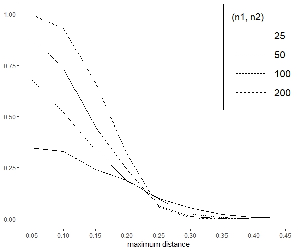
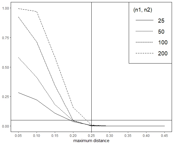
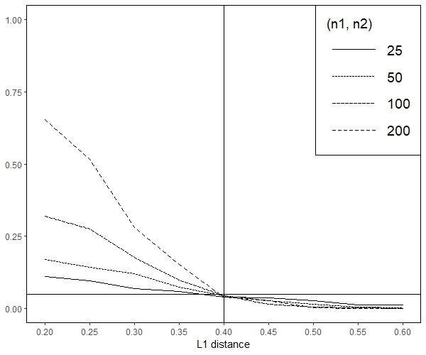
Figure 1: Simulated rejection probabilities of the test (2.5). Upper part: maximum deviation $\|\cdot\|_{\infty}$ for the probability vectors (3.1) (left) and (3.2) (right). Lower part: $L^{1}$-distance $\|\cdot\|_{1}$ for the probability vectors (3.3) (left) and (3.4) (right).

4 Appendix: Proof of Theorem 2.1

First, we prove a key lemma that is used for the proof of (2.6). For this purpose we introduce the notations $\theta=p-q$, $\hat{\hat{\theta}}=\hat{\hat{p}}-\hat{\hat{q}}$, $\hat{\theta}^{*}=\hat{p}^{*}-\hat{q}^{*}$, $\hat{d}^{*}=\|\hat{\theta}^{*}\|$, $\hat{\hat{d}}=\|\hat{\hat{\theta}}\|$ and denote the data by $\mathcal{Y}$.

Lemma 4.1

Define $\tilde{T}_{n}^{*}:=d_{\theta}^{\prime}(\sqrt{n}(\hat{\theta}^{*}-\hat{\hat{\theta}}))$, then $\tilde{T}_{n}^{*}\xrightarrow{d}T$ conditionally on $\mathcal{Y}$ in probability, and

$$\sqrt{n}(\hat{d}^{*}-\hat{\hat{d}})\leq\tilde{T}_{n}^{*}+o_{\mathbb{P}}(1).$$ (4.1)

Proof of Lemma 4.1:.

We know that

$$\sqrt{n}(\hat{\hat{\theta}}-\theta)\xrightarrow{d}Z\leavevmode\nobreak\ ,\leavevmode\nobreak\ \leavevmode\nobreak\ \sqrt{n}(\hat{\theta}^{*}-\hat{\hat{\theta}})\xrightarrow{d}Z\quad\text{conditionally on $\mathcal{Y}$.}$$ (4.2)

By the same arguments as given in the proof of Theorem 23.9 in Van der Vaart, (1998), we obtain that both sequences $\sqrt{n}(\hat{\hat{\theta}}-\theta)$ and $\sqrt{n}(\hat{\theta}^{*}-\theta)$ converge unconditionally in distribution. Applying the delta method for directionally Hadamard differentiable functions (see Theorem 2.1 in Fang and Santos, (2019)), we therefore obtain for both sequences

$$\sqrt{n}(\|\hat{\hat{\theta}}\|-\|\theta\|)=d_{\theta}^{\prime}(\sqrt{n}(\hat{\hat{\theta}}-\theta))+o_{\mathbb{P}}(1).$$

$$\sqrt{n}(\|\hat{\theta}^{*}\|-\|\theta\|)=d_{\theta}^{\prime}(\sqrt{n}(\hat{\theta}^{*}-\theta))+o_{\mathbb{P}}(1).$$

Subtracting the first equation from the second and then using sub-additivity of the directional Hadamard derivative yields

$$\sqrt{n}(\hat{d}^{*}-\hat{\hat{d}}) =\sqrt{n}(\|\hat{\theta}^{*}\|-\|\hat{\hat{\theta}}\|)$$

$$=d_{\theta}^{\prime}(\sqrt{n}(\hat{\theta}^{*}-\theta))-d_{\theta}^{\prime}(\sqrt{n}(\hat{\theta}^{*}-\theta))+o_{\mathbb{P}}(1)\leq\tilde{T}_{n}^{*}\ +\ o_{\mathbb{P}}(1).$$

Finally, the latter convergence in (4.2) together with the continuous mapping theorem yield $\tilde{T}_{n}^{*}\xrightarrow{d}T$ (note that the directional Hadamard derivative is continuous, see for example Proposition 3.1 in Shapiro, (1990) ). ∎

We continue showing the following two preliminary results that are used for the remainder of the proof:

$$\forall\delta>0:\lim_{n\to\infty}\mathbb{P}\big{(}\sqrt{n}(\hat{q}_{\alpha}^{*}-\hat{\hat{d}})>q_{\alpha+\delta}\big{)}=0.$$ (4.3)

$$\lim_{n\to\infty}\mathbb{P}\big{(}\hat{\hat{d}}<\hat{q}_{\alpha}^{*}\big{)}=0,$$ (4.4)

where $q_{\alpha}$ denotes the $\alpha$-quantile of $T$.

Proof of (4.3) and (4.4).

Let $F_{n}$ be the distribution function of $\tilde{T}_{n}^{*}$ conditional on the data and $F_{n}^{*}$ be the distribution function of $\sqrt{n}(\hat{d}^{*}-\hat{\hat{d}})$ conditional on the data.

By assumption $q_{\alpha}<0$ and therefore there exists a $t_{0}<0$ with $F(t_{0})<\alpha$. Since $\tilde{T}_{n}^{*}\xrightarrow{d}T$ conditionally on $\mathcal{Y}$ in probability, we get $\sup_{t\geq t_{0}}|F_{n}(t)-F(t)|\xrightarrow{\mathbb{P}}0.$ From (4.1) we can conclude $\mathbb{P}(F_{n}^{*}(t)\geq F_{n}(t-\epsilon)\ \forall t)\xrightarrow{n\to\infty}1$ for all $\epsilon>0$. Since $F$ is uniformly continuous on $[t_{0},\infty)$, we therefore obtain

$$\forall\epsilon>0:\ \mathbb{P}(F_{n}^{*}(t)\geq F(t)-\epsilon\ \forall t\geq t_{0})\xrightarrow{n\to\infty}1.$$ (4.5)

Now, let $\delta>0$ be arbitrary. Since $F(t_{0})<\alpha$, we have $q_{\alpha+\delta}>t_{0}$. The convergence (4.5) then yields in particular for $t=q_{\alpha+\delta}$ and $\epsilon=\delta/3$ that

$$\mathbb{P}(F_{n}^{*}(q_{\alpha+\delta})<F(q_{\alpha+\delta})-\delta/3)=\mathbb{P}(F_{n}^{*}(q_{\alpha+\delta})<\alpha+(2/3)\delta)\xrightarrow{n\to\infty}0.$$ (4.6)

Therefore, we can conclude that

$$\mathbb{P}(\sqrt{n}(\hat{q}_{\alpha}^{*}-\hat{\hat{d}})>q_{\alpha+\delta}) \leq\mathbb{P}(F_{n}^{*}(\sqrt{n}(\hat{q}_{\alpha}^{*}-\hat{\hat{d}}))\geq F_{n}^{*}(q_{\alpha+\delta}))$$

$$=\mathbb{P}(\alpha\geq F_{n}^{*}(q_{\alpha+\delta}))\leq\mathbb{P}(F_{n}^{*}(q_{\alpha+\delta})<\alpha+(2/3)\delta)=o(1),$$

which proves (4.3). For a proof of (4.4) note that we have assumed $q_{\alpha}<0$. Therefore we can choose $\delta>0$ small enough such that $q_{\alpha+\delta}<0$ as well which gives, observing (4.3),

$$\mathbb{P}(\hat{\hat{d}}<\hat{q}_{\alpha}^{*})=\mathbb{P}(\sqrt{n}(\hat{q}_{\alpha}^{*}-\hat{\hat{d}})>0)\leq\mathbb{P}(\sqrt{n}(\hat{q}_{\alpha}^{*}-\hat{\hat{d}})>q_{\alpha+\delta})\xrightarrow{n\to\infty}0.$$

∎

Using (4.3) and (4.4), we can now complete the proof of Theorem 2.1 starting with part (a). If $d>\epsilon$, we use

$$\mathbb{P}(\hat{d}<\hat{q}_{\alpha}^{*})=\mathbb{P}(\hat{d}<\hat{q}_{\alpha}^{*},\ \hat{d}\geq\epsilon)+\mathbb{P}(\hat{d}<\hat{q}_{\alpha}^{*},\ \hat{d}<\epsilon).$$

The first term satisfies $\mathbb{P}(\hat{d}<\hat{q}_{\alpha}^{*},\ \hat{d}\geq\epsilon)=\mathbb{P}(\hat{d}<\hat{q}_{\alpha}^{*},\ \hat{d}=\hat{\hat{d}})\leq\mathbb{P}(\hat{\hat{d}}<\hat{q}_{\alpha}^{*})\xrightarrow{n\to\infty}0,$ by (4.4). The second term satisfies

$$\mathbb{P}(\hat{d}<\hat{q}_{\alpha}^{*},\ \hat{d}<\epsilon)\leq\mathbb{P}(\hat{d}<\epsilon)=\mathbb{P}(\sqrt{n}(\hat{d}-d)<\sqrt{n}(\epsilon-d))\xrightarrow{n\to\infty}0,$$

since $\sqrt{n}(\hat{d}-d)$ converges weakly by the directional delta method and $\sqrt{n}(\epsilon-d)\xrightarrow{n\to\infty}-\infty$ by the assumption $d>\epsilon$. All in all, this gives $\lim_{n\to\infty}\mathbb{P}(\hat{d}<\hat{q}_{\alpha}^{*})=0$, if $d>\epsilon$.

In the case $d=\epsilon$ we use

$$\mathbb{P}(\hat{d}<\hat{q}_{\alpha}^{*})=\mathbb{P}(\hat{d}<\hat{q}_{\alpha}^{*},\ \hat{\hat{d}}=\epsilon)+\mathbb{P}(\hat{d}<\hat{q}_{\alpha}^{*},\ \hat{\hat{d}}>\epsilon).$$

To deal with the first term we introduce the notation $\hat{p}_{\alpha}^{*}:=\sqrt{n}(\hat{q}_{\alpha}^{*}-\hat{\hat{d}})$ and obtain for any $\delta>0$

$$\mathbb{P}(\hat{d}<\hat{q}_{\alpha}^{*},\ \hat{\hat{d}}=\epsilon) =\mathbb{P}(\sqrt{n}(\hat{d}-d)<\sqrt{n}(\hat{q}_{\alpha}^{*}-\hat{\hat{d}}),\ \hat{\hat{d}}=\epsilon)$$

$$\leq\mathbb{P}(\sqrt{n}(\hat{d}-d)<\sqrt{n}(\hat{q}_{\alpha}^{*}-\hat{\hat{d}}))$$

$$=\mathbb{P}(\sqrt{n}(\hat{d}-d)<\hat{p}_{\alpha}^{*},\ \hat{p}_{\alpha}^{*}\leq q_{\alpha+\delta})+\mathbb{P}(\sqrt{n}(\hat{d}-d)<\hat{p}_{\alpha}^{*},\ \hat{p}_{\alpha}^{*}>q_{\alpha+\delta})\leavevmode\nobreak\ .$$ (4.7)

For the first sequence in (4.7), we have

$$\mathbb{P}(\sqrt{n}(\hat{d}-d)<\hat{p}_{\alpha}^{*},\ \hat{p}_{\alpha}^{*}\leq q_{\alpha+\delta})\leq\mathbb{P}(\sqrt{n}(\hat{d}-d)\leq q_{\alpha+\delta})\xrightarrow{n\to\infty}\alpha+\delta,$$ (4.8)

by the weak convergence of $\sqrt{n}(\hat{d}-d)$ and since the limit distribution function is continuous at $q_{\alpha+\delta}$. For the second term in (4.7), we have

$$\mathbb{P}(\sqrt{n}(\hat{d}-d)<\hat{p}_{\alpha}^{*},\ \hat{p}_{\alpha}^{*}>q_{\alpha+\delta})\leq\mathbb{P}(\hat{p}_{\alpha}^{*}>q_{\alpha+\delta})\xrightarrow{n\to\infty}0,$$ (4.9)

by (4.3). Putting (4.8) and (4.9) together, we obtain $\limsup_{n\to\infty}\mathbb{P}(\hat{d}<\hat{q}_{\alpha}^{*})\leq\alpha+\delta\leavevmode\nobreak\$ for any $\delta>0$. This is equivalent to $\limsup_{n\to\infty}\mathbb{P}(\hat{d}<\hat{q}_{\alpha}^{*})\leq\alpha$, which completes the proof of part (a).

The proof of part (b) follows by similar arguments as given in the proof of Theorem 2 in Dette et al., (2018) (note that the map $(p,q)\to\|p-q\|$ is uniformly continuous).

For a proof of part (c), we first determine the asymptotic distribution of the bootstrap test statistic $\hat{d}^{*}$. To this end, recall that the second convergence in (4.2) holds, that is $\sqrt{n}(\hat{\theta}^{*}-\hat{\hat{\theta}})\xrightarrow{d}Z$ conditionally on $\mathcal{Y}$ in probability. Since we assume that the directional Hadamard derivative of the norm $\|\cdot\|$ is linear, we can apply the bootstrap delta method for Hadamard differentiable functions as stated in Theorem 23.9 in Van der Vaart, (1998) in order to obtain

$$\sqrt{n}(\|\hat{\theta}^{*}\|-\|\hat{\hat{\theta}}\|)\xrightarrow{d}d_{\theta}^{\prime}(Z)$$ (4.10)

conditionally on $\mathcal{Y}$ in probability. Employing the convergences (2.3) and (4.10), we can now proceed with exactly the same arguments as given in the proof of Theorem 3.3 a) cases 1 and 2 in Dette et al., (2018) in order to finish the proof.

Acknowledgements: This research is supported by the European Union through the European Joint Programme on Rare Diseases under the European Union’s Horizon 2020 Research and Innovation Programme Grant Agreement Number 825575.

References

- Alba-Fernández and Jiménez-Gamero, (2023) Alba-Fernández, M. V. and Jiménez-Gamero, M. D. (2023). Equivalence tests for multinomial data based on -divergences, pages 121–129. Springer International Publishing, Cham.
- Bogachev, (1998) Bogachev, V. I. (1998). Gaussian measures. Number 62. American Mathematical Society.
- Cárcamo et al., (2020) Cárcamo, J., Cuevas, A., and Rodríguez, L.-A. (2020). Directional differentiability for supremum-type functionals: Statistical applications. Bernoulli, 26(3):2143 – 2175.
- Dette et al., (2018) Dette, H., Möllenhoff, K., Volgushev, S., and Bretz, F. (2018). Equivalence of regression curves. Journal of the American Statistical Association, 113(522):711–729.
- Fang and Santos, (2019) Fang, Z. and Santos, A. (2019). Inference on directionally differentiable functions. The Review of Economic Studies, 86(1):377–412.
- Frey, (2009) Frey, J. (2009). An exact multinomial test for equivalence. Canadian Journal of Statistics, 37(1):47–59.
- Ostrovski, (2017) Ostrovski, V. (2017). Testing equivalence of multinomial distributions. Statistics & Probability Letters, 124:77–82.
- Ostrovski, (2018) Ostrovski, V. (2018). Testing equivalence to families of multinomial distributions with application to the independence model. Statistics & Probability Letters, 139:61–66.
- Shapiro, (1990) Shapiro, A. (1990). On concepts of directional differentiability. Journal of optimization theory and applications, 66:477–487.
- Shapiro, (1991) Shapiro, A. (1991). Asymptotic analysis of stochastic programs. Annals of Operations Research, 30(1):169–186.
- Van der Vaart, (1998) Van der Vaart, A. W. (1998). Asymptotic Statistics. Cambridge Series in Statistical and Probabilistic Mathematics. Cambridge University Press, Cambridge.
- Wellek, (2010) Wellek, S. (2010). Testing statistical hypotheses of equivalence and noninferiority. CRC Press.