Universal solution for optimal protocols of finite-time and weak processes

Abstract

The analytical expression for the optimal protocol of the thermodynamic work and its variance for finite-time, isothermal and weak processes is presented. The method that solves the Euler-Lagrange integral equation is quite general and depends only on the properties of time-reversal symmetry of the optimal protocol. The solution is proven to be physically consistent and many examples are solved to illustrate the method. To overcome the hypothesis consistency problem of the singular part of the solution, an interpretation of the appearance of the delta peaks and their derivatives is presented.

I Introduction

In times when computational endeavor has achieved its maximum power, a detriment in the search for simple analytical methods is a severe symptom. Scientific analyses restrain themselves in case-to-case examples and generalizations, which without a doubt is an important part of every scientific investigation, become a herculean task. That is the case for instance of problems that depend on methods to solve integral equations, which rely basically on the analysis of types of kernels and equations [1].

In such a scenario, it was quite disappointing to attack the problem of finding the optimal protocols of the thermodynamic work and its variance in finite-time and weak processes [2], since its Euler-Lagrange integral equation was of the worst type possible – Fredholm integral equation of first kind and constant limits of integration –, and highly depend on the kernel proposed [3]. Alternative methods, like genetic programming, although they present a result with some easiness, predicted in some cases optimal protocols outside the range of linear-response theory, which would defy its utility for this case.

This work tries to solve all the complications described above by solving the Euler-Lagrange integral equation of the referred problem in a general way. The method is quite general and depends only on the symmetric property of the optimal protocol, which was already found in previous work [3]. I find that the optimal protocol, for any reasonable physical system in the regime proposed, is universal, being composed of a straight line with jumps at the beginning and end of the process, and a series of Dirac deltas and their derivatives. Also, it depends exclusively on the ratio between the switching time of the process and the relaxation timescale of the system. To illustrate the method, I present many examples, from Brownian motion to the Ising chain, whose results corroborate the approach. Finally, to overcome the problem if the singular part of the equation is in accord with the hypothesis of linear response theory, an interpretation of the appearance of the Dirac deltas and their derivatives is presented.

II Preliminaries

I start defining notations and developing the main concepts to be used in this work.

Consider a classical system with a Hamiltonian $\mathcal{H}(\mbox{\boldmath$z$}(\mbox{\boldmath$z_{0}$},t)),\lambda(t))$, where $\mbox{\boldmath$z$}(\mbox{\boldmath$z_{0}$},t)$ is a point in the phase space $\Gamma$ evolved from the initial point $z_{0}$ until time $t$, with $\lambda(t)$ being a time-dependent external parameter. During a switching time $\tau$, the external parameter is changed from $\lambda_{0}$ to $\lambda_{0}+\delta\lambda$, with the system being in contact with a heat bath of temperature $\beta\equiv{(k_{B}T)}^{-1}$, where $k_{B}$ is Boltzmann’s constant. The average work performed on the system during this interval of time is

$$\overline{W}\equiv\int_{0}^{\tau}\left\langle\overline{\partial_{\lambda}\mathcal{H}}(t)\right\rangle_{0}\dot{\lambda}(t)dt,$$ (1)

where $\partial_{\lambda}$ is the partial derivative in respect to $\lambda$ and the superscripted dot the total time derivative. The generalized force $\left\langle\overline{\partial_{\lambda}\mathcal{H}}\right\rangle_{0}$ is calculated using the averaging $\overline{\cdot}$ over the stochastic path and the averaging $\langle\cdot\rangle_{0}$ over the initial canonical ensemble. The external parameter can be expressed as

$$\lambda(t)=\lambda_{0}+g(t)\delta\lambda,$$ (2)

where, to satisfy the initial conditions of the external parameter, the protocol $g(t)$ must satisfy the following boundary conditions

$$g(0)=0,\quad g(\tau)=1.$$ (3)

We consider as well that $g(t)\equiv g(t/\tau)$, which means that the intervals of time are measured according to the switching time unit.

Linear-response theory aims to express average quantities until the first-order of some perturbation parameter considering how this perturbation affects the observable to be averaged and the process of average [4]. In our case, we consider that the parameter does not considerably changes during the process, $|g(t)\delta\lambda/\lambda_{0}|\ll 1$, for all $t\in[0,\tau]$. In that manner, using such framework, the generalized force can be approximated until first-order as

$$\begin{split}\left\langle\overline{\partial_{\lambda}\mathcal{H}}(t)\right\rangle_{0}=&\,\left\langle\partial_{\lambda}\mathcal{H}\right\rangle_{0}+\delta\lambda\left\langle\partial_{\lambda\lambda}^{2}\mathcal{H}\right\rangle_{0}g(t)\\ &-\delta\lambda\int_{0}^{t}\phi_{0}(t-t^{\prime})g(t^{\prime})dt^{\prime}.\end{split}$$ (4)

The quantity $\phi_{0}(t)$ is the so-called response function [4], which can be conveniently expressed as the derivative of the relaxation function $\Psi_{0}(t)$ [4]

$$\phi_{0}(t)=-\frac{d\Psi_{0}}{dt}.$$ (5)

In our particular case, the relaxation function is calculated as

$$\Psi_{0}(t)=\beta\left\langle\partial_{\lambda}\mathcal{H}(0)\overline{\partial_{\lambda}\mathcal{H}}(t)\right\rangle_{0}-\mathcal{C},$$ (6)

where the constant $\mathcal{C}$ is calculated to vanish the relaxation function for long times [4]. We define as the relaxation timescale of the system the quantity

$$\tau_{R}=\int_{0}^{\infty}\frac{\Psi(t)}{\Psi(0)}dt.$$ (7)

The generalized force, written in terms of the relaxation function, can be expressed as

$$\begin{split}\left\langle\overline{\partial_{\lambda}\mathcal{H}}(t)\right\rangle_{0}=&\,\left\langle\partial_{\lambda}\mathcal{H}\right\rangle_{0}-\delta\lambda\widetilde{\Psi}_{0}g(t)\\ &+\delta\lambda\int_{0}^{t}\Psi_{0}(t-t^{\prime})\dot{g}(t^{\prime})dt^{\prime},\end{split}$$ (8)

where $\widetilde{\Psi}_{0}\equiv\Psi_{0}(0)-\left\langle\partial_{\lambda\lambda}^{2}\mathcal{H}\right\rangle_{0}$. Finally, combining Eqs. (1) and (8), the average work performed at the linear response of the generalized force is

$$\begin{split}\overline{W}=&\,\delta\lambda\left\langle\partial_{\lambda}\mathcal{H}\right\rangle_{0}-\frac{\delta\lambda^{2}}{2}\widetilde{\Psi}_{0}\\ &+\delta\lambda^{2}\int_{0}^{\tau}\int_{0}^{t}\Psi_{0}(t-t^{\prime})\dot{g}(t^{\prime})\dot{g}(t)dt^{\prime}dt.\end{split}$$ (9)

We observe that the double integral on Eq. (9) vanishes for long switching times [5]. Therefore the other terms are part of the contribution of the difference of free energy, since this quantity is exactly the average work performed for quasistatic processes in isothermal drivings. Thus, we can split the average work into the difference of free energy $\Delta F$ and irreversible work $W_{\rm irr}$

$$\Delta F=\delta\lambda\left\langle\partial_{\lambda}\mathcal{H}\right\rangle_{0}-\frac{\delta\lambda^{2}}{2}\widetilde{\Psi}_{0},$$ (10)

$$\begin{split}W_{\text{irr}}=\delta\lambda^{2}\int_{0}^{\tau}\int_{0}^{t}\Psi_{0}(t-t^{\prime})\dot{\lambda}(t^{\prime})\dot{\lambda}(t)dt^{\prime}dt.\end{split}$$ (11)

In particular, the irreversible work can be rewritten using the symmetric property of the relaxation function [4]

$$\begin{split}W_{\rm irr}=\frac{\delta\lambda^{2}}{2}\int_{0}^{\tau}\int_{0}^{\tau}\Psi_{0}(t-t^{\prime})\dot{\lambda}(t^{\prime})\dot{\lambda}(t)dt^{\prime}dt.\end{split}$$ (12)

I establish at this point the regimes where linear-response theory is able to describe thermodynamic processes. Those regimes are determined by the relative strength of the driving with respect to the initial value of the protocol, $\delta\lambda/\lambda_{0}$, and the rate by which the process occurs with respect to the relaxation time of the system, $\tau_{R}/\tau$. See Fig. 1 for a diagram depicting the regimes. In region 1, the so-called slowly-varying processes, the ratio $\delta\lambda/\lambda_{0}$ is arbitrary, while $\tau_{R}/\tau\ll 1$. By contrast, in region 2, the so-called finite-time and weak processes, the ratio $\delta\lambda/\lambda_{0}\ll 1$, while $\tau_{R}/\tau$ is arbitrary. In region 3, the so-called arbitrarily far-from-equilibrium processes, both ratios are arbitrary. Linear-response theory can only describe regions 1 and 2 [5]. In this work, we are going to focus on region 2 only.

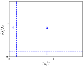
Figure 1: (Color online) Diagram of nonequilibrium regions. Region 1: slowly-varying processes, Region 2: finite-time but weak processes and Region 3: arbitrarily far-from-equilibrium processes. Linear response theorem can describe regions 1 and 2.

Consider the irreversible work rewritten in terms of the protocols $g(t)$ instead of its derivative

$$W_{\rm irr}= \frac{\delta\lambda^{2}}{2}\Psi(0)+\delta\lambda^{2}\int_{0}^{\tau}\dot{\Psi}_{0}(\tau-t)g(t)dt$$ (13)

$$-\frac{\delta\lambda^{2}}{2}\int_{0}^{\tau}\int_{0}^{\tau}\ddot{\Psi}(t-t^{\prime})g(t)g(t^{\prime})dtdt^{\prime}.$$ (14)

Using calculus of variations, we can derive the Euler-Lagrange equation that furnishes the optimal protocol $g^{*}(t)$ of the system that will minimize the irreversible work [3]

$$\int_{0}^{\tau}\ddot{\Psi}_{0}(t-t^{\prime})g^{*}(t^{\prime})dt^{\prime}=\dot{\Psi}_{0}(\tau-t).$$ (15)

In particular, the optimal irreversible work will be [3]

$$W_{\rm irr}^{*}=\frac{\delta\lambda^{2}}{2}\Psi(0)+\frac{\delta\lambda^{2}}{2}\int_{0}^{\tau}\dot{\Psi}_{0}(\tau-t)g^{*}(t)dt.$$ (16)

Also, the Euler-Lagrange equation (15) furnishes also the optimal protocol that minimizes the variance of the work [2]. In this case, the optimal variance of work is

$$\sigma_{\rm W}^{2^{*}}=\frac{\beta\delta\lambda^{2}}{4}\Psi(0)+\frac{\beta\delta\lambda^{2}}{4}\int_{0}^{\tau}\dot{\Psi}_{0}(\tau-t)g^{*}(t)dt.$$ (17)

The objective of this work is to solve the Euler-Lagrange equation (15) for any kind of relaxation function of isothermal processes. Mathematically speaking, I will present a new method to solve Fredholm integral equations of the first type for symmetric kernels. Such a method relies only on the time-reversal symmetry property of the solution.

III Universal solution

To derive the universal solution of Eq. (15), I will basically use the symmetric property of the optimal protocol

$$g^{*}(t)=1-g^{*}(\tau-t).$$ (18)

First, I open the right-hand side of Eq. (15) in the appropriate integrals

$$\int_{0}^{t}\ddot{\Psi}(t-t^{\prime})g^{*}(t^{\prime})dt^{\prime}+\int_{t}^{\tau}\ddot{\Psi}(t-t^{\prime})g^{*}(t^{\prime})dt^{\prime}=\dot{\Psi}(\tau-t)$$ (19)

Using the symmetric property (18) in the second term of the right-hand side of Eq. (19), one can show that

$$\int_{0}^{t}\ddot{\Psi}(t-t^{\prime})g^{*}(t^{\prime})dt^{\prime}=\int_{0}^{\tau-t}\ddot{\Psi}(\tau-t-t^{\prime})g^{*}(t^{\prime})dt^{\prime}.$$ (20)

Therefore, Eq. (20) must be equal to a symmetric function $h(t)$, such that, $h(t)=h(\tau-t)$. Using the solution of the Euler-Lagrange equation, the above result is equal to

$$\int_{0}^{t}\ddot{\Psi}(t-t^{\prime})g^{*}(t^{\prime})dt^{\prime}=\int_{0}^{t}\ddot{\Psi}(t-t^{\prime})(1-g^{*}(\tau-t^{\prime}))dt^{\prime},$$ (21)

which is another way to express the symmetry of the optimal protocol. Consider, by simplicity, a function $g_{0}(t)$, such that

$$\int_{0}^{t}\ddot{\Psi}(t-t^{\prime})g_{0}(t^{\prime})dt^{\prime}=C_{0},$$ (22)

where $C_{0}$ is a constant in time. Applying the convolution theorem we have

$$g_{0}(t)=\mathcal{L}^{-1}_{s}\left\{\frac{C_{0}}{s\mathcal{L}_{t}\{\ddot{\Psi}(t)\}(s)}\right\}(t),$$ (23)

where $\mathcal{L}_{t}\{\cdot\}$ and $\mathcal{L}_{s}^{-1}\{\cdot\}$ are respectively the Laplace and inverse Laplace transform. Assuming that $\mathcal{L}_{t}\{\Psi(t)\}(s)$ can be expressed as a Taylor series in $s=0$, we have by applying Horner-Ruffini method

$$\frac{1}{\mathcal{L}_{t}\{\ddot{\Psi}(t)\}(s)}=\frac{1}{s^{2}\mathcal{L}_{t}\{\Psi(t)\}(s)-s\Psi(0)}=\sum_{n=-2}^{\infty}a_{n}s^{n}.$$ (24)

We have then as solution

$$g_{0}(t)=C_{0}\left(a_{-2}t+a_{-1}+\sum_{n=0}^{\infty}a_{n}\delta^{(n)}(t)\right).$$ (25)

We demand that the constant $C_{0}$ must be equal to a number where it holds the time-reversal symmetry

$$g_{0}(t)-C_{0}\sum_{n=0}^{\infty}a_{n}\delta^{(n)}(\tau-t)=1-g_{0}(\tau-t)+C_{0}\sum_{n=0}^{\infty}a_{n}\delta^{(n)}(t).$$ (26)

Since the Dirac deltas and their derivatives will cancel out, the constant will be

$$C_{0}=\frac{1}{a_{-2}\tau+2a_{-1}}.$$ (27)

In this manner, the optimal protocol, by construction, will be

$$g^{*}(t)=\frac{1}{2}\left(g_{0}(t)+1-g_{0}(\tau-t)+\right.$$ (28)

$$\left.C_{0}\sum_{n=0}^{\infty}a_{n}(\delta^{(n)}(t)-\delta^{(n)}(\tau-t))\right),$$ (29)

in which, by substituting Eq. (25) and (27), we will have

$$g^{*}(t)=-\frac{t-a_{-1}}{a_{-2}\tau+2a_{-1}}-\sum_{n=0}^{\infty}\frac{a_{n}(\delta^{(n)}(t)-\delta^{(n)}(\tau-t))}{a_{-2}\tau+2a_{-1}},$$ (30)

which is the main result of this work. As expected, such a solution shows, by the definitions of the terms $a_{n}$ that compose it, that the optimal protocol is very related to the relaxation function of the system.

IV Examples

To illustrate the consistency of the method, I find the optimal protocols of many examples of physical systems performing an isothermal process by using the procedure above.

IV.1 Overdamped Brownian motion

We consider in this example a white noise overdamped Brownian motion subjected to a time-dependent harmonic potential, with the mass of the system equal to one, $\gamma$ as a damping coefficient and $\omega_{0}$ as the natural frequency of the potential. The relaxation function for both moving laser and stiffening traps [3] are given by

$$\Psi(t)=\Psi_{0}\exp{\left(-\frac{|t|}{\tau_{R}}\right)},$$ (31)

where $\tau_{R}$ is the relaxation timescale of each case. Applying the method, the terms $a_{n}$ will be

$$a_{-2}=-1,\quad a_{-1}=-\tau_{R},\quad a_{n}=0,\,n\geq 0.$$ (32)

Therefore

$$g^{*}(t)=\frac{t+\tau_{R}}{\tau+2\tau_{R}},$$ (33)

which was first calculated by Schmiedl and Seifert [6] for the full dynamics, but which is identical to the linear-response regime [3].

IV.2 Underdamped Brownian motion

We consider in this example a white noise overdamped Brownian motion subjected to a time-dependent harmonic potential, with $m$ as the mass of the particle, $\gamma$ as a damping coefficient, and $\omega_{0}$ as the natural frequency of the potential. The relaxation function for moving laser trap [3] is given by

$$\Psi(t)=\Psi_{0}\exp{\left(-\frac{\gamma}{2}|t|\right)}\left(\cos{\omega t}+\frac{\gamma}{2\omega}\sin{\omega|t|}\right),$$ (34)

where $\omega=\sqrt{\omega_{0}^{2}-\gamma^{2}/4}$. Applying the method, the terms $a_{n}$ will be

$$a_{-2}=-1,\quad a_{-1}=-\tau_{R},\quad a_{0}=1/\omega_{0}^{2},\quad a_{n}=0,\,n\geq 1.$$ (35)

Therefore, the optimal protocol will be

$$g^{*}(t)=\frac{t+\tau_{R}}{\tau+2\tau_{R}}+\frac{\tau_{R}(\delta(t)-\delta(\tau-t))}{\gamma(\tau+2\tau_{R})},$$ (36)

where $\tau_{R}$ is the relaxation timescale of the system. This result was first calculated by Gomez-Marin and co-authors for the full dynamics [7], but which is identical to the linear-response regime.

For the stiffening trap case, the relaxation function is [5]

$$\Psi(t)=\Psi_{0}\exp{\left(-\gamma|t|\right)}\left[\frac{2\omega_{0}^{2}}{\omega^{2}}\right.\\ \left.+\left(\frac{\omega^{2}-2\omega_{0}^{2}}{\omega^{2}}\right)\cos{\omega t}+\frac{\gamma}{\omega}\sin{\omega|t|}\right],$$ (37)

where $\omega=\sqrt{4\omega_{0}^{2}-\gamma^{2}}$. The coefficients $a_{n}$ will be

$$a_{-2}=-1,\quad a_{-1}=-\tau_{R},\quad$$ (38)

$$a_{n-2}=-\frac{1}{n!}\frac{\partial^{n}}{\partial s^{n}}\frac{(s+\gamma)(s^{2}+2\gamma s+4\omega_{0}^{2})}{2\gamma(2\gamma+s)}\Big{|}_{s=0},$$ (39)

for $n\geq 2$, where $\tau_{R}$ is the relaxation timescale of the system. The optimal protocol will be

$$g^{*}(t)=\frac{t+\tau_{R}}{\tau+2\tau_{R}}+\sum_{n=0}^{\infty}\frac{a_{n}(\delta^{(n)}(t)-\delta^{(n)}(\tau-t))}{\tau+2\tau_{R}}.$$ (40)

IV.3 Sinc relaxation function

In Ref. [8], when we apply the method of time average in a thermally isolated system performing an adiabatic process, we produce a new one performing an isothermal one with a typical relaxation time. In particular, for thermally isolated systems that have a relaxation function equal to

$$\Psi(t)=\Psi_{0}\cos{(\omega t)},$$ (41)

will have for time-averaged relaxation function

$$\overline{\Psi}(t)=\Psi_{0}\,\text{sinc}\left(\frac{\pi}{2}\frac{t}{\tau_{R}}\right),$$ (42)

where $\tau_{R}$ is the relaxation timescale of the system. Applying the method, the terms $a_{n}$ will be

$$a_{-2}=-1,\quad a_{-1}=-\tau_{R},$$ (43)

$$a_{n-2}=\frac{1}{n!}\frac{\partial^{n}}{\partial s^{n}}\frac{1}{(-1+2\tau_{R}s\,\text{acot}(2\tau_{R}s/\pi)/\pi)}\Big{|}_{s=0},\,n\geq 2.$$ (44)

The optimal protocol will be

$$g^{*}(t)=\frac{t+\tau_{R}}{\tau+2\tau_{R}}+\sum_{n=0}^{\infty}\frac{a_{n}(\delta^{(n)}(t)-\delta^{(n)}(\tau-t))}{\tau+2\tau_{R}}.$$ (45)

IV.4 Gaussian relaxation function

A relaxation function that satisfies the criteria of compatibility with the Second Law of Thermodynamics [5] is the Gaussian relaxation function

$$\Psi(t)=\Psi_{0}\exp\left(-\frac{\pi}{4}\left(\frac{t}{\tau_{R}}\right)^{2}\right),$$ (46)

where $\tau_{R}$ is the relaxation timescale of the system. Applying the method, the terms $a_{n}$ will be

$$a_{-2}=-1,\quad a_{-1}=-\tau_{R},$$ (47)

and

$$a_{n-2}=\frac{1}{n!}\frac{\partial^{n}}{\partial s^{n}}\frac{1}{(-1+\tau_{R}s\exp(\tau_{R}^{2}s^{2}/\pi)\text{Erfc}(\tau_{R}s/\sqrt{\pi})}\Big{|}_{s=0},$$ (48)

for $n\geq 2$. Here $\text{Erfc}(x)$ is the complementary error function. The optimal protocol will be

$$g^{*}(t)=\frac{t+\tau_{R}}{\tau+2\tau_{R}}+\sum_{n=0}^{\infty}\frac{a_{n}(\delta^{(n)}(t)-\delta^{(n)}(\tau-t))}{\tau+2\tau_{R}}.$$ (49)

IV.5 Bessel relaxation function

The Bessel relaxation function is given by

$$\Psi(t)=\Psi_{0}J_{0}\left(\frac{t}{\tau_{R}}\right),$$ (50)

where $J_{0}$ is the Bessel function of the first kind with $\nu=0$ and $\tau_{R}$ is its relaxation timescale. It satisfies the criteria for compatibility with the Second Law of Thermodynamics. Such relaxation function can model the Ising chain subjected to a time-dependent magnetic field and evolving in time at equilibrium accordingly to Glauber-Ising dynamics [9]. Applying the method, the terms $a_{n}$ will be

$$a_{-2}=-1,\quad a_{-1}=-\tau_{R},$$ (51)

and

$$a_{n-2}=-\frac{1}{n!}\frac{\partial^{n}}{\partial s^{n}}\frac{1}{(1+\tau_{R}^{2}s^{2}+\tau_{R}s\sqrt{1+\tau_{R}^{2}s^{2}})}\Big{|}_{s=0},$$ (52)

with $n\geq 2$. The optimal protocol will be

$$g^{*}(t)=\frac{t+\tau_{R}}{\tau+2\tau_{R}}+\sum_{n=0}^{\infty}\frac{a_{n}(\delta^{(n)}(t)-\delta^{(n)}(\tau-t))}{\tau+2\tau_{R}}.$$ (53)

V Discussion

V.1 Continuous part

For all examples treated here, the continuous part of the optimal protocol $g^{*}_{C}(t)$ was given by

$$g^{*}_{C}(t)=\frac{t+\tau_{R}}{\tau+2\tau_{R}}.$$ (54)

Such a solution is consistent with previous results for extreme cases where $\tau\gg\tau_{R}$ and $\tau\ll\tau_{R}$ [3], where

$$\lim_{\tau\gg\tau_{R}}g^{*}_{C}(t)=\frac{t}{\tau},\quad\lim_{\tau\ll\tau_{R}}g^{*}_{C}(t)=\frac{1}{2}.$$ (55)

Also, this continuous part is restrained

$$0\leq g^{*}_{C}(t)\leq 1,$$ (56)

for all $t\in[0,\tau]$, $0\leq\tau/\tau_{R}\leq\infty$, meaning that it can be used in linear-response theory. Therefore, the solution is physically consistent.

V.2 Singular part

For all examples treated here, the singular part of the optimal protocol $g^{*}_{C}(t)$ was given by

$$g^{*}_{S}(t)=\sum_{n=0}^{\infty}\frac{b_{n}\tau_{R}^{n}(\delta^{(n)}(t)-\delta^{(n)}(\tau-t))}{\tau+2\tau_{R}}.$$ (57)

where $b_{n}$ is a number independent of $\tau/\tau_{R}$. For extreme cases where $\tau\gg\tau_{R}$ and $\tau\ll\tau_{R}$, we have

$$\lim_{\tau\gg\tau_{R}}g^{*}_{S}(t)=0,\quad\lim_{\tau\ll\tau_{R}}g^{*}_{C}(t)=0.$$ (58)

Another important point is the behavior of the value of the Dirac deltas and their derivatives calculated at the extreme points $t=0$ and $t=\tau$. First, I consider the Dirac delta defined as

$$\frac{d\Theta}{dt}=\delta(t),$$ (59)

where $\Theta(t)$ is the Heaviside theta function, which makes its value and the values of its derivatives calculated at $t=0$ free of choice. In order to satisfy the time-reversal symmetry (26), one must choose

$$\delta^{(n)}(0)=\delta^{(n)}(\tau),$$ (60)

for any $n\in\mathcal{N}$. Since $\tau$ is a positive number, then $\delta^{(n)}(0)=\delta^{(n)}(\tau)=0$. In particular, it is expected too that the integral of the optimal protocol must be time-reversal symmetric. Therefore, one must have

$$\Theta(0)=\Theta(\tau)=1.$$ (61)

Also, will the Dirac deltas be outside the hypothesis of linear response theory? To answer this question is necessary to understand how can one implement such delta peaks in practice in the laboratory. In my opinion, operating protocols considering “peaks” to infinity and considering “peaks” in the derivatives does not make any sense. How can one guarantee the optimality of the irreversible work then? I suggest just including the constant term calculated with the singular part in the definition of the irreversible work, whose primary definition was made considering only jumps at the beginning and final point of the process. The new optimal irreversible work will become

$$W_{\rm irr}^{*} =\ \frac{\delta\lambda^{2}}{2}\Psi(0)+\frac{\delta\lambda^{2}}{2}\int_{0}^{\tau}\dot{\Psi}_{0}(\tau-t)g^{*}(t)dt$$ (62)

$$+\frac{\delta\lambda^{2}}{2}\sum_{n=0}^{\infty}\frac{a_{n}(-1)^{n}[\dot{\Psi}^{(n)}(\tau)+\dot{\Psi}^{(n)}(0)]}{\tau+2\tau_{R}},$$ (63)

where the continuous part of the optimal protocol is now the unique part of the optimal protocol. So, in practice, the Dirac deltas are nothing more than artifices that the method of solving the integral equation presents to taking into account the terms that have been not defined in the treatment of the irreversible work, where the constants terms that appear from the Dirac deltas and its derivatives were not considered. In this manner, the Dirac deltas and derivatives are in accord to the hypothesis of linear response theory.

VI Final remarks

In this work, I presented a method to solve the Euler-Lagrange integral equation that furnishes the optimal protocol for the irreversible work and its variance. It relies only on the time-reversal symmetric property of the optimal protocol. Many examples are solved to illustrate the consistency of the method. The solution is proven to be physically consistent. To overcome the hypothesis consistency problem with the linear response theory of the singular part, an interpretation of the appearance of delta peaks is presented, where the constant terms of such singular solutions should be included at irreversible work at the beginning of the optimization problem.