Thermal analysis of photon–like particles in rainbow gravity

Abstract

This work is devoted to study the thermodynamic behavior of photon–like particles within the rainbow gravity formalism. To to do this, we chose two particular ansatzs to accomplish our calculations. First, we consider a dispersion relation which avoids UV divergences, getting a positive effective cosmological constant. We provide numerical analysis for the thermodynamic functions of the system and bounds are estimated. Furthermore, a phase transition is also expected for this model. Second, we consider a dispersion relation employed in the context of Gamma Ray Bursts. Remarkably, for this latter case, the thermodynamic properties are calculated in an analytical manner and they turn out to depend on the harmonic series $H_{n}$, gamma $\Gamma(z)$, polygamma $\psi_{n}(z)$ and zeta Riemann functions $\zeta(z)$.

I Introduction

Rainbow gravity is a promising approach for creating self–consistent cosmological models that evade singularities majumder2013singularity , which lack clear definitions within the framework of quantum gravity kangal2022effective ; kangal2021relativistic ; r1 ; r2 ; r3 ; r4 ; r5 ; r6 ; r8 ; r9 . The choice of rainbow functions can lead to varying predictions regarding the evolution of the universe, including acceleration of cosmic expansion sefiedgar2017entropic ; brighenti2017primordial ; nojiri2007introduction ; amelino2013rainbow ; sefiedgar2018thermodynamics . In this manner, exploring a diverse range of them is essential for both fundamental physics and cosmology mota2019combined ; younesizadeh2021new ; fomin2020exact . Through this investigation, we can gain new perspectives on the behavior of the universe and deepen our understanding of the intricate interplay between quantum gravity and cosmology, potentially leading to novel results and approaches for understanding the fundamental nature of our universe.

The study of thermodynamics in the context of quantum gravity is essential for comprehending the behavior of physical systems under the effects of modifications to the dispersion relation, including those described by rainbow gravity dehghani2018thermal ; dehghani2019thermodynamic ; sefiedgar2017thermodynamics ; haldar2019thermodynamics ; hamil2022effect ; kim2016thermodynamic ; dehghani2018thermodynamics ; araujo2021bouncing ; sefiedgar2018thermodynamics . The non–trivial thermodynamic properties resulting from these modifications can include changes to the thermodynamic equation of state, the critical temperature, the emergence of novel phase transitions and modifications to the Bose–Einstein condensation feng2017thermodynamic ; dehghani2020ads4 ; md2018phase ; Furtado:2021aod .

In addition, this exploration is of significant interest, particularly for its implications for black hole behavior. One of the key consequences of the modification of the dispersion relation in this framework is the emergence of a minimum length scale nilsson2017energy ; roy2023entropy , which leads to modifications of both the Hawking temperature and the entropy of black holes feng2020rainbow ; yekta2019joule . As a result, new proposals have arisen for black hole thermodynamics, including modified entropy–area relations and first laws of thermodynamics feng2018rainbow ; sefiedgar2017entropic ; sefiedgar2016can . These novel ideas offer a fresh perspective on the behavior of black holes and could potentially pave the way for a deeper understanding of them.

Here, we study the thermodynamic behavior of photon–like particles within the rainbow gravity formalism. To to do this, we chose two particular ansatzs to accomplish our calculations. First, we consider a dispersion relation which avoids UV divergences, getting a positive effective cosmological constant. To this case, we provide numerical analysis for the thermodynamic functions of the system. Also, new bounds are estimated and a phase transition is expected to our model, being highlighted by the heat capacity behavior. Second, we consider a dispersion relation employed in the context of Gamma Ray Bursts, which present a remarkable feature: analytical results. The thermal quantities turn out to depend on the following special functions: harmonic series $H_{n}$, gamma $\Gamma(z)$, polygamma $\psi_{n}(z)$ and zeta Riemann functions $\zeta(z)$.

This paper is organized as follows: in Sec. II, we briefly present the modified rainbow dispersion relation. In section III, we investigate the thermodynamic properties for two rainbow functions and new bounds are estimated. Finally, in section IV, we outline our conclusion.

II The modified dispersion relation

The general dispersion relation of massive particles in the context of Double special relativity reads amelino2001testable ; amelino2002relativity

$$E^{2}g_{1}^{2}(E/E_{P})-k^{2}g_{2}^{2}(E/E_{P})=m^{2},$$ (1)

where $g_{1}(E/E_{P})$ and $g_{2}(E/E_{P})$ are simply arbitrary functions whose the following conditions must be satisfied

$$\lim_{E/E_{P}\rightarrow 0}g_{1}(E/E_{P})=1,\,\,\,\,\,\,\text{and}\,\,\,\,\,\,\lim_{E/E_{P}\rightarrow 0}g_{2}(E/E_{P})=1.$$ (2)

Notice that the usual dispersion relation is recovered when low energy regime is considered. The first ideas of Double special relativity were developed to flat spacetimes. Nevertheless, it is not prohibited to consider a more general curved background, accounting for general relativity. Within this viewpoint, Magueijo and Smolin magueijo2004gravity suggested that the Einstein’s field equations as well as the stress–energy tensor should be modified by introducing a new parameter to the following equations

$$G_{\mu\nu}(E)=8\pi G(E)T_{\mu\nu}(E)+g_{\mu\nu}\Lambda(E),$$ (3)

where $G_{\mu\nu}$ is the Einstein tensor and $G_{\mu\nu}=R_{\mu\nu}-\frac{1}{2}Rg_{\mu\nu}$, being $R_{\mu\nu}$ the Ricci curvature tensor and $R$ the scalar curvature; $\Lambda(E)$ and $G(E)$ are the energy–dependent cosmological and Newtons constant respectively. $G(0)$ can also be defined as the usual low–energy Newton constant. In a similar manner, we may also have the line element of the rainbow–like Schwarzschild black hole

$$\mathrm{d}s^{2}=-\left(1-\frac{2MG(0)}{r}\right)\frac{\mathrm{d}t^{2}}{g_{1}^{2}(E/E_{P})}+\frac{\mathrm{d}r^{2}}{(1-2MG(0)/r)g_{2}^{2}(E/E_{P})}+\frac{r^{2}(\mathrm{d}\theta^{2}+\sin^{2}\theta\mathrm{d}\phi^{2})}{g_{2}^{2}(E/E_{P})}.$$ (4)

Since the effects of $g_{1}(E/E_{P})$ and $g_{2}(E/E_{P})$ are highlighted when the energy $E$ is similar to $E_{P}$, they modify the ultraviolet behavior analogous to what happens to the non–commutative geometry scenarios and the generalized uncertainty principle. If its modification plays a role in the Liouville measure $\mathrm{d}^{3}x\mathrm{d}^{3}k$, Eq. (4) may naturally gives rise to ultraviolet regulator. This feature is brought about due to the presence of appropriate choices of functions $g_{1}(E/E_{P})$ and $g_{2}(E/E_{P})$. Corroborating these arguments, a notable results have been obtained, applying, rainbow gravity to the black hole entropy garattini2010modified . In this reference, the UV regulator, called “the brick wall”, has been removed by considering the following choice of $g_{1}(E/E_{P})$ and $g_{2}(E/E_{P})$: $g_{1}(E/E_{P})/g_{2}(E/E_{P})=\exp[-E/E_{P}]$. Nevertheless, as it has been argued in Ref. garattini2011modified , this particular choice turns out to give us a negative effective cosmological constant. In order to overcome this situation, we shall provide our investigations based on another dispersion relation that “cure” such an issue. This and other feats will be discussed with more details in the next section.

III Thermodynamic properties

III.1 The first case

As pointed out in Refs. garattini2005casimir ; garattini2006cosmological , there exists an appearance of an induced cosmological constant $\Lambda/8\pi G$. However, it does not address neither a renormalization nor a regularization for the sake of avoiding UV divergences. Notice that if one takes into account the pure Gaussian regulator only, one verifies that the zero point energy is fundamentally negative for rainbow gravity garattini2011modified . Nevertheless, after some parametrizations, Ref. garattini2011modified got a positive value to the effective cosmological constant among other features by using the following ansatz:

$$g_{2}(E/E_{P})=1,\phantom{a}g_{1}(E/E_{P})=\sum^{n}_{i=0}\xi_{i}\left(\frac{E}{E_{P}}\right)^{i}\exp\left(-\alpha\frac{E^{2}}{E^{2}_{P}}\right)\phantom{a}\forall\phantom{a}\alpha>0,\xi_{i}\in\mathbb{R}.$$ (5)

It is exactly with above expression that we shall focus on in order to provide our calculations. Next, combining Eq. (1) with Eq. (5), we obtain

$$E^{2}\left[\sum^{n}_{i=0}\xi_{i}\left(\frac{E}{E_{P}}\right)^{i}\exp\left(-\alpha\frac{E^{2}}{E^{2}_{P}}\right)\right]^{2}-k^{2}=m^{2}.$$ (6)

Although we have presented a general modified dispersion relation, to perform our calculation, we shall particularize it, namely, $m=0$ (massless particles) and $i=0$. In other words, we shall focus on the simplest massless case. Such a case leads to the following partition function

$$\ln[Z]=-\frac{1}{2}\ln\left(1-e^{-\beta E}\right)\left(2E\xi_{0}^{2}e^{-\frac{2\alpha E^{2}}{E_{P}^{2}}}-\frac{4\alpha E^{3}\xi_{0}^{2}e^{-\frac{2\alpha E^{2}}{E_{P}^{2}}}}{E_{P}^{2}}\right)\sqrt{E^{2}\xi_{0}^{2}e^{-\frac{2\alpha E^{2}}{E_{P}^{2}}}},$$ (7)

where $\beta\equiv 1/\kappa_{B}T$, and $\kappa_{B}$ is the Boltzmann constant. After that, all thermodynamic quantities can be addressed. It is important to note that, from now on, the thermodynamic properties will be calculated, taking into account the following constant values $\xi_{0}=\alpha=1$.

III.1.1 Equation of states

In this subsection, we focus on the study of the equation of states. Then, it reads

$$P=-\int^{\infty}_{0}\frac{\ln\left(1-e^{-\beta E}\right)}{2\beta}\sqrt{\xi_{0}^{2}E^{2}e^{-\frac{2\alpha E^{2}}{E_{P}^{2}}}}\left(2\xi_{0}^{2}Ee^{-\frac{2\alpha E^{2}}{E_{P}^{2}}}-\frac{4\alpha\xi_{0}^{2}E^{3}e^{-\frac{2\alpha E^{2}}{b^{2}}}}{E_{P}^{2}}\right)\mathrm{d}E.$$ (8)

Here, we notice that we have $lim_{\alpha\rightarrow\infty}P=0$, and

$$\lim_{\alpha\rightarrow 0}P=\frac{\pi^{4}}{45}\left(\xi_{0}^{2}\right){}^{3/2}T^{4}=\frac{\pi^{2}}{3}\sigma\left(\xi_{0}^{2}\right){}^{3/2}T^{4}=\tilde{\alpha}T^{4},$$ (9)

where $\tilde{\alpha}=\pi^{2}\sigma\left(\xi_{0}^{2}\right){}^{3/2}/3$ and $\sigma$ is the well–known Stefan–Boltzmann constant given by

$$\sigma=\frac{1}{\pi^{2}}\int^{\infty}_{0}\frac{E^{3}\,e^{-\beta E}}{\left(1-e^{-\beta E}\right)}\mathrm{d}E=\frac{\pi^{2}}{15}.$$ (10)

It is important to highlight, even considering such limits to the massive case, the integral did not converge. This is why we opted to work on the massless particles instead in this manuscript. Also, Eq. (9) gives rise to a modified Stefan–Boltzmann law. As we may probably realize, Eq. (8) does not possess analytical results. To overcome this issue, we provide a numerical analysis as seen in Fig. 1. This thermodynamic property is a monotonically increasing function for different values of temperature $T$. Also, Fig. 1 provides a clear visualization of the impact of rainbow gravity in pressure as temperature increase compared to the conventional case where the effects of rainbow gravity are disregarded. Notably, the disparity between the two cases is more pronounced at higher temperatures, which is expected as therainbow gravity influence becomes increasingly significant at elevated energy levels.

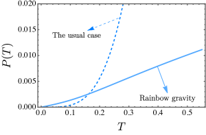
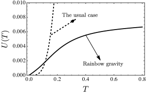
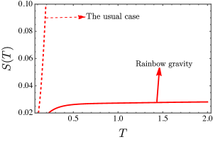
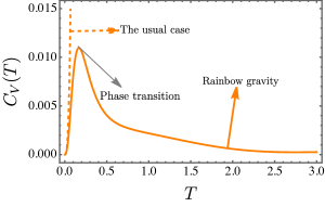
Figure 1: All thermodynamic state quantities for different values of temperature $T$. The point that the pressures coincide is $T=0.11$ GeV; also, the point the mean energies coincide is $T=0.16$ GeV.

III.1.2 Mean energy

Here, we investigate the main aspects of the mean energy for our system. In addition, the black body radiation can also be examined as well in possession of this thermal state quantity. With this purpose, we write

$$U=\int^{\infty}_{0}\frac{Ee^{-\beta E}}{2\left(1-e^{-\beta E}\right)}\left(2E\xi_{0}^{2}e^{-\frac{2\alpha E^{2}}{E_{P}^{2}}}-\frac{4\alpha E^{3}\xi_{0}^{2}e^{-\frac{2\alpha E^{2}}{E_{P}^{2}}}}{E_{P}^{2}}\right)\sqrt{E^{2}\xi_{0}^{2}e^{-\frac{2\alpha E^{2}}{E_{P}^{2}}}}\mathrm{d}E.$$ (11)

It is worthy to be mentioned that $lim_{\alpha\rightarrow\infty}U=0$, and $lim_{\alpha\rightarrow 0}U$ results

$$\lim_{\alpha\rightarrow 0}U=\frac{\pi^{4}}{15}\left(\xi_{0}^{2}\right){}^{3/2}T^{4}=\pi^{2}\sigma\left(\xi_{0}^{2}\right){}^{3/2}T^{4}=\bar{\alpha}T^{4},$$ (12)

where $\bar{\alpha}\equiv\pi^{2}\sigma\left(\xi_{0}^{2}\right){}^{3/2}$. Similarly with what happened to the equation of states, here, we have recovered the Stefan–Boltzmann law after redefining the constants. For a more robust analysis besides this one given by this particular limit, we show a numerical analysis to the mean energy. The results are shown in Fig. 1. As we can see from the plot, the mean energy increases its values when the temperature varies until tending to reach a constant behavior at $T>0.8$ GeV, which contrast to the usual mean energy behavior, i.e., monotonically increasing function. More so, in a straightforward manner, from Eq. (12), we can also obtain the associated black body radiation

$$\chi(\alpha,\upsilon)=\frac{h\nu e^{-\beta h\nu}}{2\left(1-e^{-\beta h\nu}\right)}\left(2h\nu\xi_{0}^{2}e^{-\frac{2\alpha h\nu^{2}}{E_{P}^{2}}}-\frac{4\alpha h\nu^{3}\xi_{0}^{2}e^{-\frac{2\alpha h\nu^{2}}{E_{P}^{2}}}}{E_{P}^{2}}\right)\sqrt{h\nu^{2}\xi_{0}^{2}e^{-\frac{2\alpha h\nu^{2}}{E_{P}^{2}}}},$$ (13)

where $h$ is the Planck constant and $\nu$ is the frequency. The corresponding behavior of such a quantity is displayed in Fig. 2. It is worth highlighting that one of the parameters which account for the rainbow gravity, namely, $\alpha$, plays an important role in the shape of the black body radiation. Furthermore, if the following limit is considered $\lim_{\alpha\rightarrow 0}X$, we obtain

$$\lim_{\alpha\rightarrow 0}X=\frac{(h\nu)^{2}\xi_{0}^{2}e^{-\beta h\nu}\sqrt{(h\nu)^{2}\xi_{0}^{2}}}{1-e^{-\beta h\nu}}.$$ (14)

Notice that, if parameter $\xi_{0}\rightarrow 1$, the usual well–known result encountered in the literature for the black body radiation is recovered.

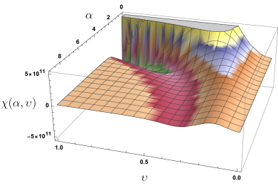
Figure 2: The black body radiation for different values of $\alpha$ and $\upsilon$.

Now let us estimate a bound for the $\xi_{0}$ parameter comparing to some black body radiation spectrum. Let us consider that $\xi_{0}\approx 1+\delta\xi_{0}$, so that

$$U\approx\pi^{2}\sigma\left[(1+\delta\xi_{0})^{2}\right]{}^{3/2}T^{4}\approx\pi^{2}\sigma T^{4}+3\pi^{2}\sigma\delta\xi_{0}T^{4}.$$ (15)

Based on the above expansion, let us now try to find a bound to $\delta\xi_{0}$. To do so, we suppose the contribution of $\delta\xi_{0}$ is less than the observational error. From Ref. BBRadiations , we can make such an estimation via the microwave background radiation using black body radiation inversion:

$$\delta\xi_{0}\leq 1.50\times 10^{-12}.$$ (16)

III.1.3 Entropy

The entropy in this section will be discussed. It reads

$$\begin{split}S=&\int^{\infty}_{0}\beta^{2}\left[\frac{Ee^{-\beta E}\sqrt{E^{2}\xi_{0}^{2}+e^{-\frac{2\alpha E^{2}}{E_{P}^{2}}}}\left(2E\xi_{0}^{2}e^{-\frac{2\alpha E^{2}}{E_{P}^{2}}}-\frac{4\alpha E^{3}\xi_{0}^{2}e^{-\frac{2\alpha E^{2}}{E_{P}^{2}}}}{E_{P}^{2}}\right)}{2\beta\left(1-e^{-\beta E}\right)}\right.\\ &\left.-\frac{\ln\left(1-e^{-\beta E}\right)\sqrt{E^{2}\xi_{0}^{2}+e^{-\frac{2\alpha E^{2}}{E_{P}^{2}}}}\left(2E\xi_{0}^{2}e^{-\frac{2\alpha E^{2}}{E_{P}^{2}}}-\frac{4\alpha E^{3}\xi_{0}^{2}e^{-\frac{2\alpha E^{2}}{E_{P}^{2}}}}{E_{P}^{2}}\right)}{2\beta^{2}}\right]\mathrm{d}E.\end{split}$$ (17)

Analogously what we have done with the previous thermodynamic functions, we take into account $lim_{\alpha\rightarrow\infty}S=0$, and $lim_{\alpha\rightarrow 0}S$ leads to

$$S=\frac{4\pi^{4}}{45}\left(\xi_{0}^{2}\right){}^{3/2}T^{3}.$$ (18)

In order to obtain a general panorama, we provide numerical analysis to this thermodynamic state function as well, whose the plot is shown in Fig. 1. Here, we clearly see that this thermodynamic quantity almost reaches a constant behavior in comparison with the usual case, which is a monotonically increasing function to different values of temperature $T$.

III.1.4 Heat capacity

Finally, to complete our investigation, we supply the last thermal function, the heat capacity. In this sense, we can write it as

$$\begin{split}C_{V}=&\int^{\infty}_{0}\beta^{2}\left[\frac{E^{2}e^{-2\beta E}\sqrt{E^{2}\xi_{0}^{2}+e^{-\frac{2\alpha E^{2}}{E_{P}^{2}}}}\left(2E\xi_{0}^{2}e^{-\frac{2\alpha E^{2}}{E_{P}^{2}}}-\frac{4\alpha E^{3}\xi_{0}^{2}e^{-\frac{2\alpha E^{2}}{E_{P}^{2}}}}{E_{P}^{2}}\right)}{2\left(1-e^{-\beta E}\right)^{2}}\right.\\ &\left.+\frac{E^{2}e^{-\beta E}\sqrt{E^{2}\xi_{0}^{2}+e^{-\frac{2\alpha E^{2}}{E_{P}^{2}}}}\left(2E\xi_{0}^{2}e^{-\frac{2\alpha E^{2}}{E_{P}^{2}}}-\frac{4\alpha E^{3}\xi_{0}^{2}e^{-\frac{2\alpha E^{2}}{E_{P}^{2}}}}{E_{P}^{2}}\right)}{2\left(1-e^{-\beta E}\right)}\right]\mathrm{d}E.\end{split}$$ (19)

Next, we consider $lim_{\alpha\rightarrow\infty}C_{V}=0$, and $lim_{\alpha\rightarrow 0}C_{V}$ leads to

$$C_{V}=\frac{4\pi^{4}}{15}\left(\xi_{0}^{2}\right){}^{3/2}T^{3}.$$ (20)

Now, we supply a numerical analysis to heat capacity, which is exhibited in Fig. 1. In comparison with the previous thermal quantity, an analogous behavior also occurs to the usal case: the existence of an monotonically increasing function when the temperature $T$ runs. Nevertheless, to the rainbow case we verify that actually does exist a phase transition for $T=0.167$ GeV, i.e., at the point $(0.167,0.010)$; and the second law of thermodynamics is still maintained araujo2023thermodynamics ; furtado2023thermodynamical . It worth commenting that the similar studies have also appeared in the literature recently aa1 ; aa2 ; aa3 ; aa4 ; aa5 ; aa6 ; aa7 ; aa8 ; aa9 ; aa10 ; aa11 ; aa12 ; aa13 ; aa14 .

III.2 The second case

The selection of next rainbow functions was initially explored in 51 within the framework of Gamma Ray Bursts. Later, this particular choice of rainbow functions was further studied with respect to its application to FRW solutions 52 ; 53 .

Here, we present the subsequent ansazts that we shall use to perform our calculation

$$g_{1}(E/E_{P})=\frac{e^{\frac{E\xi}{E_{P}}}-1}{\frac{E\xi}{E_{P}}},\,\,\,\,\,\,g_{2}(E/E_{P})=1.$$ (21)

Similarly to what we have done in the previous section, now we shall investigate the thermodynamic behavior of the latter case present in Eq. (21). To this case, the partition function reads

$$\ln[Z_{2}]=-\int^{\infty}_{0}\frac{E_{P}^{2}}{\xi^{2}}e^{\frac{E\xi}{E_{P}}}\left(e^{\frac{E\xi}{E_{P}}}-1\right)^{2}\ln\left(1-e^{-\beta E}\right)\mathrm{d}E.$$ (22)

III.2.1 Equation of states

The study of the equation of states in the context of rainbow gravity is motivated by the need to understand how gravity behaves under the influence of quantum effects. They characterize the behavior of matter and energy in a gravitational system. By studying it in the context of rainbow gravity, we aim to gain insights into the nature of gravity at the quantum level. With this, we can possibly address new phenomenology for describing the behavior of black holes and neutron stars for instance. In this sense, the equation of states are straightforwardly derived as

$$\begin{split}P_{2}(T)&=-\int^{\infty}_{0}\frac{E_{P}}{\beta\xi^{2}}e^{\frac{E\xi}{E_{P}}}\left(e^{\frac{E\xi}{E_{P}}}-1\right)\sqrt{a^{2}\left(e^{\frac{E\xi}{E_{P}}}-1\right)^{2}}\ln\left(1-e^{-\beta E}\right)\mathrm{d}E\\ &=-\frac{E_{P}^{3}\left(3H_{-\frac{\xi}{E_{P}\beta}}-3H_{-\frac{2\xi}{E_{P}\beta}}+H_{-\frac{3\xi}{E_{P}\beta}}\right)}{3\beta\xi^{3}},\end{split}$$ (23)

where $H_{n}$ is the harmonic series defined by

$$H_{n}=\sum_{n}^{k=1}\frac{1}{k}.$$ (24)

In Fig. 3, we display the behavior of $P_{2}(T)$. Due to the harmonic series characteristic, the pressure shows discontinuity in its shape. The presence of such a discontinuity might be seen as a signal that the current assumption or ansatz for the rainbow functions is not physically valid within this context. As we shall see, a similar periodic discontinuity is also evident in other thermodynamic quantities.

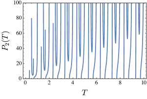
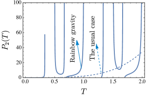
Figure 3: Pressure for different values of temperature $T$, considering the second case.

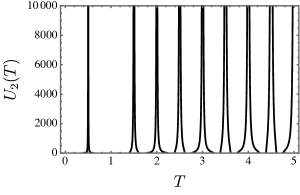
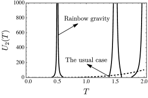
Figure 4: Mean energy for different values of temperature $T$, considering the second case.

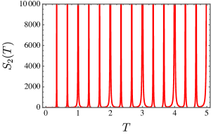
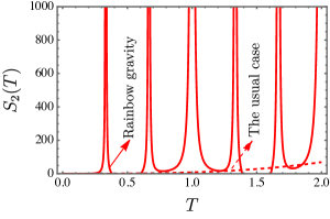
Figure 5: Entropy for different values of temperature $T$, considering the second case.

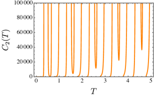
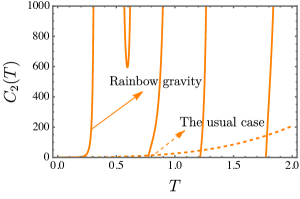
Figure 6: Heat capacity for different values of temperature $T$, considering the second case.

III.2.2 Mean energy

Understanding the behavior of particles at extremely high energy scales is a crucial area of research in physics, with important implications for our understanding of the universe. Studying the mean energy of an ensemble of particles in the context of rainbow gravity can provide valuable insights into the distribution of energy among particles and the nature of spacetime at these scales. This can help us better understand the effects of quantum gravity and inform the development of new applications. Then, the mean energy reads,

$$\begin{split}U_{2}(T)=&\int_{0}^{\infty}\frac{E_{P}^{2}E\left(e^{\frac{E\xi}{E_{P}}}-1\right)^{2}e^{\frac{E\xi}{E_{P}}-\beta E}}{\xi^{2}\left(1-e^{-\beta E}\right)}\,\mathrm{d}E\\ &=\frac{E_{P}^{2}\left(\psi_{1}\left(1-\frac{\xi}{E_{P}\beta}\right)-2\psi_{1}\left(1-\frac{2\xi}{E_{P}\beta}\right)+\psi_{1}\left(1-\frac{3\xi}{E_{P}\beta}\right)\right)}{\beta^{2}\xi^{2}},\end{split}$$ (25)

where $\psi_{n}(z)$ is the pollygamma function defined by the derivative of the logarithm of the gamma function $\Gamma(z)\equiv\int^{\infty}_{0}t^{z-1}e^{-t}\mathrm{d}t$, which can explicitly given by

$$\psi_{n}(z)=\frac{\mathrm{d}^{n+1}}{\mathrm{d}z^{n+1}}\ln[\Gamma(z)]=(-1)^{n+1}n!\sum^{\infty}_{k=0}\frac{1}{(z+k)^{n+1}}=(-1)^{n+1}n!\zeta(n+1,z),\,\,\,\,\forall n>0,$$ (26)

with $\zeta(a,z)$ being the Hurwitz zeta function. Notice that, if we consider the limit where $\xi\rightarrow 0$, we obtain $\lim_{\xi\rightarrow 0}U_{2}(T)=\pi^{4}T^{4}/15$, recovering also the well–known Stefan–Boltzmann law. Also, if the temperature $T\rightarrow\infty$, $\lim_{T\rightarrow 0}U_{2}(T)=0$.

Special functions, have been used to analyze the thermodynamic properties of various systems, including black holes, and Bose–Einstein condensation (BEC) phase transition, and. For instance, in Refs. b1 ; b2 ; b3 ; b4 , the authors used the ensemble theory to analyze a trapped Bose gas, and calculated the thermodynamic potentials and critical temperature for BEC. In addition, they have also been used to study the the thermodynamical properties in different scenarios of gravitational theories, such as Gauss–Bonnet cvetivc2002black , higher curvature gravities myers1988black ; lov2 ; lov3 , holography dong2014holographic ; hollogra , and charged black holes zou2014critical .

Very recently in the literature, $\psi_{n}(z)$ has also been employed to address an arbitrary number of dipoles at the sites of a regular one–dimensional crystal lattice ciftja2023exact , geometric study of fluctuating $1/2$–BPS statistical configurations bellucci2010exact , Tsales statistics niven2009q , expansion of the one-loop corrections klajn2014exact , correspondence between thermodynamics and inference lamont2019correspondence , double wrapping in twisted AdS/CFT, Five loop Konishi from AdS/CFT bajnok2010five , thermodynamics of Gaussian fluctuations and paraconductivity in layered superconductorsmishonov2000thermodynamics , Kurtosis of von Neumann entanglement entropyhuang2021kurtosis , and macroscopically ordered water in nanopores kofinger2008macroscopically , and gas–liquid transition in the system of dipolar hard spheres levin1999happened .

In Fig. 4, the behavior the the mean energy might possibly indicate either quantum fluctuations of the massless particles or an extreme phase transition in this scenario.

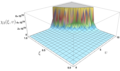
Figure 7: The black body radiation for different values of $\xi$ and $\upsilon$.

III.2.3 Entropy

The study of entropy in the context of rainbow gravity is a crucial area of research in physics, as it provides a unique perspective on the behavior of particles in extreme conditions. By analyzing the distribution of entropy among particles, we can gain a deeper understanding of the fundamental nature of spacetime and its underlying quantum structure. This knowledge has important implications for the development of new theories of physics, as well as for practical applications in fields such as quantum computing and information theory. Moreover, studying the entropy of particle ensembles may provide novel perspectives on the behavior of matter and energy in high–energy regimes, which can ultimately lead to groundbreaking discoveries and advancements in our understanding of the universe. The entropy reads

$$\begin{split}&S_{2}(T)=\int_{0}^{\infty}\beta^{2}\left(\frac{E_{P}^{2}E\left(e^{\frac{E\xi}{E_{P}}}-1\right)^{2}e^{\frac{E\xi}{E_{P}}-\beta E}}{\beta\xi^{2}\left(1-e^{-\beta E}\right)}-\frac{E_{P}^{2}e^{\frac{E\xi}{E_{P}}}\left(e^{\frac{E\xi}{E_{P}}}-1\right)^{2}\log\left(1-e^{-\beta E}\right)}{\beta^{2}\xi^{2}}\right)\,\mathrm{d}E\\ &=\frac{E_{P}^{2}}{36\xi^{2}}\left(-\frac{18\beta^{2}E_{P}^{3}}{(E_{P}\beta-2\xi)\xi^{2}}+\frac{4\beta^{2}E_{P}^{3}}{(E_{P}\beta-3\xi)\xi^{2}}-\frac{36\beta^{2}E_{P}^{3}}{\xi(\xi-E_{P}\beta)^{2}}+\frac{14\beta E_{P}^{2}}{\xi^{2}}+\frac{54\beta E_{P}^{2}}{(\xi-E_{P}\beta)^{2}}\right.\\ &\left.-\frac{36\beta E_{P}^{2}}{(E_{P}\beta-2\xi)^{2}}+\frac{18\beta E_{P}^{2}}{(E_{P}\beta-3\xi)^{2}}-\frac{36\gamma\beta E_{P}^{2}}{E_{P}\beta\xi-\xi^{2}}+\frac{72\beta E_{P}^{2}}{E_{P}\beta\xi-2\xi^{2}}-\frac{24\beta E_{P}^{2}}{E_{P}\beta\xi-3\xi^{2}}\right.\\ &\left.+\frac{36\psi_{0}\left(2-\frac{2\xi}{E_{P}\beta}\right)^{2}E_{P}}{E_{P}\beta-2\xi}+\frac{36\psi_{0}\left(-\frac{\xi}{E_{P}\beta}\right)E_{P}}{E_{P}\beta-\xi}+36\left(\frac{1}{\xi}-\frac{2}{E_{P}\beta-2\xi}\right)\psi_{0}\left(-\frac{2\xi}{E_{P}\beta}\right)E_{P}\right.\\ &\left.+\left(\frac{36}{E_{P}\beta-3\xi}-\frac{12}{\xi}\right)\psi_{0}\left(-\frac{3\xi}{E_{P}\beta}\right)E_{P}+\frac{18\gamma^{2}E_{P}}{E_{P}\beta-\xi}+\frac{3\pi^{2}E_{P}}{E_{P}\beta-\xi}-\frac{18\psi_{0}\left(2-\frac{\xi}{E_{P}\beta}\right)^{2}E_{P}}{E_{P}\beta-\xi}\right.\\ &\left.-\frac{36\psi_{0}\left(-\frac{\xi}{E_{P}\beta}\right)E_{P}}{\xi}+\frac{24\gamma E_{P}}{\xi}-\frac{36\gamma^{2}E_{P}}{E_{P}\beta-2\xi}-\frac{6\pi^{2}E_{P}}{E_{P}\beta-2\xi}+\frac{18\gamma^{2}E_{P}}{E_{P}\beta-3\xi}+\frac{3\pi^{2}E_{P}}{E_{P}\beta-3\xi}\right.\\ &\left.-\frac{18\psi_{0}\left(2-\frac{3\xi}{E_{P}\beta}\right)^{2}E_{P}}{E_{P}\beta-3\xi}+\frac{18\psi_{0}\left(1-\frac{\xi}{E_{P}\beta}\right)^{2}}{\beta}+\frac{18\xi\psi_{0}\left(2-\frac{\xi}{E_{P}\beta}\right)^{2}}{\beta(E_{P}\beta-\xi)}+\frac{18\psi_{0}\left(1-\frac{3\xi}{E_{P}\beta}\right)^{2}}{\beta}\right.\\ &\left.+\frac{54\xi\psi_{0}\left(2-\frac{3\xi}{E_{P}\beta}\right)^{2}}{\beta(E_{P}\beta-3\xi)}+\frac{36\psi_{1}\left(-\frac{\xi}{E_{P}\beta}\right)}{\beta}+\frac{36\psi_{1}\left(-\frac{3\xi}{E_{P}\beta}\right)}{\beta}-\frac{36\psi_{0}\left(1-\frac{2\xi}{E_{P}\beta}\right)^{2}}{\beta}\right.\\ &\left.-\frac{72\psi_{1}\left(-\frac{2\xi}{E_{P}\beta}\right)}{\beta}-\frac{72\xi\psi_{0}\left(2-\frac{2\xi}{E_{P}\beta}\right)^{2}}{\beta(E_{P}\beta-2\xi)}-\frac{18\gamma^{2}\xi}{E_{P}\beta^{2}-\beta\xi}-\frac{3\pi^{2}\xi}{E_{P}\beta^{2}-\beta\xi}+\frac{72\gamma^{2}\xi}{E_{P}\beta^{2}-2\beta\xi}\right.\\ &\left.+\frac{12\pi^{2}\xi}{E_{P}\beta^{2}-2\beta\xi}-\frac{54\gamma^{2}\xi}{E_{P}\beta^{2}-3\beta\xi}-\frac{9\pi^{2}\xi}{E_{P}\beta^{2}-3\beta\xi}+\frac{36\gamma E_{P}}{E_{P}\beta-\xi}\right),\end{split}$$ (27)

where, $\gamma$ is the Euler gamma defined by $\gamma=\lim_{n\rightarrow\infty}\left(\sum^{n}_{k=1}\frac{1}{k}-\ln(n)\right)$. Here, if we consider the limit where $\lim_{\xi\rightarrow 0}S_{2}(T)=T^{3}[4\pi^{4}-45\gamma(2+\psi^{(2)}(1)-\psi^{(2)}(2))+45(2+\psi^{(2)}(1)-\psi^{(2)}(2))/45]=4\pi^{4}T^{3}/45$. Also, for $\lim_{T\rightarrow 0}S_{2}(T)=0$. The behavior of the entropy for this case is displayed in Fig. 5, comparing such thermal function with the usal case.

III.2.4 Heat capacity

Finally, in this subsection we provide the study of the heat capacity. In this way, we write

$$\begin{split}C_{2}(T)&=\int_{0}^{\infty}-\beta^{2}\left(-\frac{E_{P}^{2}E^{2}\left(e^{\frac{E\xi}{E_{P}}}-1\right)^{2}e^{\frac{E\xi}{E_{P}}-\beta E}}{\xi^{2}\left(1-e^{-\beta E}\right)}-\frac{E_{P}^{2}E^{2}\left(e^{\frac{E\xi}{E_{P}}}-1\right)^{2}e^{\frac{E\xi}{E_{P}}-2\beta E}}{\xi^{2}\left(1-e^{-\beta E}\right)^{2}}\right)\,\mathrm{d}E\\ &=\frac{E_{P}}{\beta^{2}\xi^{2}}\left\{2E_{P}\beta\left[\psi_{1}\left(-\frac{\xi}{E_{P}\beta}\right)-2\psi_{1}\left(-\frac{2\xi}{E_{P}\beta}\right)+\psi_{1}\left(-\frac{3\xi}{E_{P}\beta}\right)\right]\right.\\ &\left.-\xi\left[\psi_{2}\left(-\frac{\xi}{E_{P}\beta}\right)-4\psi_{2}\left(-\frac{2\xi}{E_{P}\beta}\right)+3\psi_{2}\left(-\frac{3\xi}{E_{P}\beta}\right)\right]\right\}\end{split}$$ (28)

In addition, we have $\lim_{\rightarrow 0}C_{2}(T)=4\pi^{4}T^{3}/15$. Also, for $\lim_{T\rightarrow 0}C_{2}(T)=0$. Finally, we compare the role of rainbow parameters in comparison with the usual case. This analysis is shown in Fig. 6.

IV Conclusion

This study was devoted to studying the thermodynamic behavior of photon-like particles within the framework of rainbow gravity. To accomplish this, two particular ansatzs were chosen for conducting the calculations. Initially, a dispersion relation was considered that avoided UV divergences, resulting in a positive effective cosmological constant. Numerical analysis was performed to evaluate the thermodynamic functions of the system and estimate bounds. Furthermore, a phase transition was also observed in this model.

Next, a dispersion relation employed in the context of Gamma Ray Bursts was investigated. Interestingly, in this case, the thermodynamic properties were calculated analytically. It was found that these properties depended on various mathematical functions, such as the harmonic series $H_{n}$, gamma $\Gamma(z)$, polygamma $\psi_{n}(z)$ and zeta Riemann functions $\zeta(z)$. Overall, this work contributed to the understanding of the thermodynamics of photon–like particles within the rainbow gravity formalism. The combination of numerical and analytical approaches provided valuable insights into the behavior of the system and established connections with important mathematical functions. Further exploration of these phenomena could deepen our comprehension of fundamental physics and its implications.

As a future perspective, analyzing the role of the mass within this context seems to be a interesting question worthy to be investigated.

V Data Availability Statement

Data Availability Statement: No Data associated in the manuscript

References

- (1) B. Majumder, “Singularity free rainbow universe,” International Journal of Modern Physics D, vol. 22, no. 12, p. 1342021, 2013.
- (2) E. Kangal, K. Sogut, M. Salti, and O. Aydogdu, “Effective dynamics of spin-1/2 particles in a rainbow universe,” Annals of Physics, vol. 444, p. 169018, 2022.
- (3) E. Kangal, M. Salti, O. Aydogdu, and K. Sogut, “Relativistic quantum dynamics of scalar particles in the rainbow formalism of gravity,” Physica Scripta, vol. 96, no. 9, p. 095301, 2021.
- (4) A. F. Ali and M. M. Khalil, “A proposal for testing gravity’s rainbow,” Europhysics Letters, vol. 110, no. 2, p. 20009, 2015.
- (5) S. Gangopadhyay and A. Dutta, “Constraints on rainbow gravity functions from black-hole thermodynamics,” Europhysics Letters, vol. 115, no. 5, p. 50005, 2016.
- (6) A. Awad, A. F. Ali, and B. Majumder, “Nonsingular rainbow universes,” Journal of Cosmology and Astroparticle Physics, vol. 2013, no. 10, p. 052, 2013.
- (7) A. F. Ali, M. Faizal, B. Majumder, and R. Mistry, “Gravitational collapse in gravity’s rainbow,” International Journal of Geometric Methods in Modern Physics, vol. 12, no. 09, p. 1550085, 2015.
- (8) M. de Montigny, J. Pinfold, S. Zare, and H. Hassanabadi, “Klein–gordon oscillator in a global monopole space–time with rainbow gravity,” The European Physical Journal Plus, vol. 137, pp. 1–17, 2022.
- (9) J. Magueijo, “New varying speed of light theories,” Reports on Progress in Physics, vol. 66, no. 11, p. 2025, 2003.
- (10) G. F. Ellis, “Note on varying speed of light cosmologies,” arXiv preprint astro-ph/0703751, 2007.
- (11) G. F. Ellis and J.-P. Uzan, “c is the speed of light, isn’t it?,” American journal of physics, vol. 73, no. 3, pp. 240–247, 2005.
- (12) A. Sefiedgar, “From the entropic force to the friedmann equation in rainbow gravity,” Europhysics Letters, vol. 117, no. 6, p. 69001, 2017.
- (13) F. Brighenti, G. Gubitosi, and J. Magueijo, “Primordial perturbations in a rainbow universe with running newton constant,” Physical Review D, vol. 95, no. 6, p. 063534, 2017.
- (14) S. Nojiri and S. D. Odintsov, “Introduction to modified gravity and gravitational alternative for dark energy,” International Journal of Geometric Methods in Modern Physics, vol. 4, no. 01, pp. 115–145, 2007.
- (15) G. Amelino-Camelia, M. Arzano, G. Gubitosi, and J. Magueijo, “Rainbow gravity and scale-invariant fluctuations,” Physical Review D, vol. 88, no. 4, p. 041303, 2013.
- (16) A. Sefiedgar and M. Mirzazadeh, “Thermodynamics of the frw universe at the event horizon in palatini f(r) gravity,” Advances in High Energy Physics, vol. 2018, pp. 1–6, 2018.
- (17) C. E. Mota, L. C. Santos, G. Grams, F. M. da Silva, and D. P. Menezes, “Combined rastall and rainbow theories of gravity with applications to neutron stars,” Physical Review D, vol. 100, no. 2, p. 024043, 2019.
- (18) Y. Younesizadeh, A. H. Ahmed, A. A. Ahmad, Y. Younesizadeh, and M. Ebrahimkhas, “New class of solutions in -gravity’s rainbow and -gravity: Exact solutions thermodynamics quasinormal modes,” Nuclear Physics B, vol. 971, p. 115376, 2021.
- (19) I. Fomin and S. Chervon, “Exact and slow-roll solutions for exponential power-law inflation connected with modified gravity and observational constraints,” Universe, vol. 6, no. 11, p. 199, 2020.
- (20) M. Dehghani, “Thermal fluctuations of dilaton black holes in gravity’s rainbow,” Physics Letters B, vol. 781, pp. 553–560, 2018.
- (21) M. Dehghani, “Thermodynamic properties of novel dilatonic btz black holes under the influence of rainbow gravity,” Physics Letters B, vol. 799, p. 135037, 2019.
- (22) A. S. Sefiedgar and M. Daghigh, “Thermodynamics of the frw universe in rainbow gravity,” International Journal of Modern Physics D, vol. 26, no. 13, p. 1750139, 2017.
- (23) A. Haldar and R. Biswas, “Thermodynamics of reissner–nordstr o¨ m black holes in higher dimensions: rainbow gravity background with general uncertainty principle,” General Relativity and Gravitation, vol. 51, no. 6, p. 72, 2019.
- (24) B. Hamil and B. Lütfüoğlu, “Effect of snyder–de sitter model on the black hole thermodynamics in the context of rainbow gravity,” International Journal of Geometric Methods in Modern Physics, vol. 19, no. 03, p. 2250047, 2022.
- (25) Y.-W. Kim, S. K. Kim, and Y.-J. Park, “Thermodynamic stability of modified schwarzschild–ads black hole in rainbow gravity,” The European Physical Journal C, vol. 76, pp. 1–11, 2016.
- (26) M. Dehghani, “Thermodynamics of charged dilatonic btz black holes in rainbow gravity,” Physics Letters B, vol. 777, pp. 351–360, 2018.
- (27) A. A. Araújo Filho and A. Y. Petrov, “Bouncing universe in a heat bath,” International Journal of Modern Physics A, vol. 36, no. 34n35, p. 2150242, 2021.
- (28) Z.-W. Feng and S.-Z. Yang, “Thermodynamic phase transition of a black hole in rainbow gravity,” Physics Letters B, vol. 772, pp. 737–742, 2017.
- (29) M. Dehghani, “Ads4 black holes with nonlinear source in rainbow gravity,” Physics Letters B, vol. 801, p. 135191, 2020.
- (30) S. Md, “Phase transition of quantum-corrected schwarzschild black hole in rainbow gravity,” Physics Letters B, vol. 784, pp. 6–11, 2018.
- (31) J. Furtado, J. F. Assunção, and C. R. Muniz, “Relativistic Bose-Einstein condensate in the rainbow gravity,” EPL, vol. 139, p. 29001, 2022.
- (32) N. A. Nilsson and M. P. Dabrowski, “Energy scale of lorentz violation in rainbow gravity,” Physics of the Dark Universe, vol. 18, pp. 115–122, 2017.
- (33) T. Roy and U. Debnath, “Entropy bound and egup correction of d-dimensional reissner-nordstrom black hole in rainbow gravity,” International Journal of Modern Physics A, 2023.
- (34) Z.-W. Feng, X. Zhou, S.-Q. Zhou, and D.-D. Feng, “Rainbow gravity corrections to the information flux of a black hole and the sparsity of hawking radiation,” Annals of Physics, vol. 416, p. 168144, 2020.
- (35) D. M. Yekta, A. Hadikhani, and Ö. Ökcü, “Joule-thomson expansion of charged ads black holes in rainbow gravity,” Physics Letters B, vol. 795, pp. 521–527, 2019.
- (36) Z.-W. Feng and S.-Z. Yang, “Rainbow gravity corrections to the entropic force,” Advances in High Energy Physics, vol. 2018, 2018.
- (37) A. S. Sefiedgar, “How can rainbow gravity affect gravitational force?,” International Journal of Modern Physics D, vol. 25, no. 14, p. 1650101, 2016.
- (38) G. Amelino-Camelia, “Testable scenario for relativity with minimum length,” Physics Letters B, vol. 510, no. 1-4, pp. 255–263, 2001.
- (39) G. Amelino-Camelia, “Relativity in spacetimes with short-distance structure governed by an observer-independent (planckian) length scale,” International Journal of Modern Physics D, vol. 11, no. 01, pp. 35–59, 2002.
- (40) J. Magueijo and L. Smolin, “Gravity’s rainbow,” Classical and Quantum Gravity, vol. 21, no. 7, p. 1725, 2004.
- (41) R. Garattini, “Modified dispersion relations and black hole entropy,” Physics Letters B, vol. 685, no. 4-5, pp. 329–337, 2010.
- (42) R. Garattini and G. Mandanici, “Modified dispersion relations lead to a finite zero point gravitational energy,” Physical Review D, vol. 83, no. 8, p. 084021, 2011.
- (43) R. Garattini, “Casimir energy, the cosmological constant and massive gravitons,” arXiv preprint gr-qc/0510062, 2005.
- (44) R. Garattini, “The cosmological constant as an eigenvalue of a sturm–liouville problem and its renormalization,” Journal of Physics A: Mathematical and General, vol. 39, no. 21, p. 6393, 2006.
- (45) K. Konar, K. Bose, and R. Paul, “Revisiting cosmic microwave background radiation using blackbody radiation inversion,” Scientific Reports, vol. 11, no. 1, p. 1008, 2021.
- (46) A. A. Araújo Filho, S. Zare, P. Porfírio, J. Kříž, and H. Hassanabadi, “Thermodynamics and evaporation of a modified schwarzschild black hole in a non–commutative gauge theory,” Physics Letters B, p. 137744, 2023.
- (47) J. Furtado, J. Silva, et al., “Thermodynamical properties of an ideal gas in a traversable wormhole,” arXiv preprint arXiv:2302.05492, 2023.
- (48) R. R. Oliveira, A. A. Araújo Filho, F. C. Lima, R. V. Maluf, and C. A. Almeida, “Thermodynamic properties of an aharonov-bohm quantum ring,” The European Physical Journal Plus, vol. 134, no. 10, p. 495, 2019.
- (49) A. A. Araújo Filho and J. Reis, “Thermal aspects of interacting quantum gases in lorentz-violating scenarios,” The European Physical Journal Plus, vol. 136, pp. 1–30, 2021.
- (50) R. Oliveira et al., “Thermodynamic properties of neutral dirac particles in the presence of an electromagnetic field,” The European Physical Journal Plus, vol. 135, no. 1, pp. 1–10, 2020.
- (51) A. A. Araújo Filho, “Lorentz-violating scenarios in a thermal reservoir,” The European Physical Journal Plus, vol. 136, no. 4, pp. 1–14, 2021.
- (52) R. Oliveira, A. A. Araújo Filho, R. Maluf, and C. Almeida, “The relativistic aharonov–bohm–coulomb system with position-dependent mass,” Journal of Physics A: Mathematical and Theoretical, vol. 53, no. 4, p. 045304, 2020.
- (53) A. A. Araújo Filho and R. V. Maluf, “Thermodynamic properties in higher-derivative electrodynamics,” Brazilian Journal of Physics, vol. 51, pp. 820–830, 2021.
- (54) A. A. Araújo Filho and A. Y. Petrov, “Higher-derivative lorentz-breaking dispersion relations: a thermal description,” The European Physical Journal C, vol. 81, no. 9, p. 843, 2021.
- (55) A. A. Araújo Filho and A. Y. Petrov, “Bouncing universe in a heat bath,” International Journal of Modern Physics A, vol. 36, no. 34n35, p. 2150242, 2021.
- (56) A. A. Araújo Filho, “Thermodynamics of massless particles in curved spacetime,” arXiv preprint arXiv:2201.00066, 2022.
- (57) A. A. Araújo Filho, “Particles in loop quantum gravity formalism: a thermodynamical description,” Annalen der Physik, p. 2200383, 2022.
- (58) A. A. Araújo Filho, J. Reis, and S. Ghosh, “Fermions on a torus knot,” The European Physical Journal Plus, vol. 137, no. 5, p. 614, 2022.
- (59) A. A. Araújo Filho and J. Reis, “How does geometry affect quantum gases?,” International Journal of Modern Physics A, vol. 37, no. 11n12, p. 2250071, 2022.
- (60) P. Sedaghatnia, H. Hassanabadi, J. Porfírio, W. Chung, et al., “Thermodynamical properties of a deformed schwarzschild black hole via dunkl generalization,” arXiv preprint arXiv:2302.11460, 2023.
- (61) A. A. Araújo Filho, J. Furtado, and J. Silva, “Thermodynamical properties of an ideal gas in a traversable wormhole,” arXiv preprint arXiv:2302.05492, 2023.
- (62) G. Amelino-Camelia, J. Ellis, N. Mavromatos, D. V. Nanopoulos, and S. Sarkar, “Tests of quantum gravity from observations of -ray bursts,” Nature, vol. 393, no. 6687, pp. 763–765, 1998.
- (63) A. Awad, A. F. Ali, and B. Majumder, “Nonsingular rainbow universes,” Journal of Cosmology and Astroparticle Physics, vol. 2013, no. 10, p. 052, 2013.
- (64) G. Santos, G. Gubitosi, and G. Amelino-Camelia, “On the initial singularity problem in rainbow cosmology,” Journal of Cosmology and Astroparticle Physics, vol. 2015, no. 08, p. 005, 2015.
- (65) G. Baym and C. J. Pethick, “Ground-state properties of magnetically trapped bose-condensed rubidium gas,” Physical review letters, vol. 76, no. 1, p. 6, 1996.
- (66) E. H. Lieb and R. Seiringer, “Proof of bose-einstein condensation for dilute trapped gases,” Physical review letters, vol. 88, no. 17, p. 170409, 2002.
- (67) L. Santos, G. Shlyapnikov, P. Zoller, and M. Lewenstein, “Bose-einstein condensation in trapped dipolar gases,” Physical Review Letters, vol. 85, no. 9, p. 1791, 2000.
- (68) F. Dalfovo, S. Giorgini, L. P. Pitaevskii, and S. Stringari, “Theory of bose-einstein condensation in trapped gases,” Reviews of modern physics, vol. 71, no. 3, p. 463, 1999.
- (69) M. Cvetič, S. Nojiri, and S. D. Odintsov, “Black hole thermodynamics and negative entropy in de sitter and anti-de sitter einstein–gauss–bonnet gravity,” Nuclear Physics B, vol. 628, no. 1-2, pp. 295–330, 2002.
- (70) R. C. Myers and J. Z. Simon, “Black-hole thermodynamics in lovelock gravity,” Physical Review D, vol. 38, no. 8, p. 2434, 1988.
- (71) H. Saida and J. Soda, “Statistical entropy of btz black hole in higher curvature gravity,” Physics Letters B, vol. 471, no. 4, pp. 358–366, 2000.
- (72) S. Banerjee, A. Bhattacharyya, A. Kaviraj, K. Sen, and A. Sinha, “Constraining gravity using entanglement in ads/cft,” Journal of High Energy Physics, vol. 2014, no. 5, pp. 1–34, 2014.
- (73) X. Dong, “Holographic entanglement entropy for general higher derivative gravity,” Journal of High Energy Physics, vol. 2014, no. 1, pp. 1–32, 2014.
- (74) R.-X. Miao, “An exact construction of codimension two holography,” Journal of High Energy Physics, vol. 2021, no. 1, pp. 1–27, 2021.
- (75) D.-C. Zou, Y. Liu, and B. Wang, “Critical behavior of charged gauss-bonnet-ads black holes in the grand canonical ensemble,” Physical Review D, vol. 90, no. 4, p. 044063, 2014.
- (76) O. Ciftja, “Exact ground state energy of a system with an arbitrary number of dipoles at the sites of a regular one-dimensional crystal lattice,” Journal of Physics and Chemistry of Solids, vol. 172, p. 111044, 2023.
- (77) S. Bellucci and B. Nath Tiwari, “An exact fluctuating 1/2-bps configuration,” Journal of High Energy Physics, vol. 2010, no. 5, pp. 1–35, 2010.
- (78) R. K. Niven and H. Suyari, “The q-gamma and (q, q)-polygamma functions of tsallis statistics,” Physica A: Statistical Mechanics and its Applications, vol. 388, no. 19, pp. 4045–4060, 2009.
- (79) B. Klajn, “Exact high temperature expansion of the one-loop thermodynamic potential with complex chemical potential,” Physical Review D, vol. 89, no. 3, p. 036001, 2014.
- (80) C. H. LaMont and P. A. Wiggins, “Correspondence between thermodynamics and inference,” Physical Review E, vol. 99, no. 5, p. 052140, 2019.
- (81) Z. Bajnok, Á. Hegedűs, R. A. Janik, and T. Łukowski, “Five loop konishi from ads/cft,” Nuclear physics B, vol. 827, no. 3, pp. 426–456, 2010.
- (82) T. Mishonov and E. Penev, “Thermodynamics of gaussian fluctuations and paraconductivity in layered superconductors,” International Journal of Modern Physics B, vol. 14, no. 32, pp. 3831–3879, 2000.
- (83) Y. Huang, L. Wei, and B. Collaku, “Kurtosis of von neumann entanglement entropy,” Journal of Physics A: Mathematical and Theoretical, vol. 54, no. 50, p. 504003, 2021.
- (84) J. Köfinger, G. Hummer, and C. Dellago, “Macroscopically ordered water in nanopores,” Proceedings of the National Academy of Sciences, vol. 105, no. 36, pp. 13218–13222, 2008.
- (85) Y. Levin, “What happened to the gas-liquid transition in the system of dipolar hard spheres?,” Physical review letters, vol. 83, no. 6, p. 1159, 1999.