Bulk-Edge Correspondence for Point-Gap Topological Phases in Junction Systems

Abstract

The bulk-edge correspondence is one of the most important ingredients in the theory of topological phases of matter. While the bulk-edge correspondence is applicable for Hermitian junction systems where two subsystems with independent topological invariants are connected to each other, it has not been discussed for junction systems with non-Hermitian point-gap topological phases. In this Letter, based on analytical results obtained by the extension of non-Bloch band theory to junction systems, we establish the bulk-edge correspondence for point-gap topological phases in junction systems. We also confirm that almost all the eigenstates are localized near the interface which are called the “non-Hermitian proximity effects”. One of the unique properties is that the localization length becomes the same for both subsystems nevertheless those model-parameters are different.

Introduction. Non-Hermitian systems have recently received a lot of attention since they possess novel physical phenomena and richer topological properties than Hermitian systems[1, 2, 3, 4, 5, 6, 7, 8, 9, 10, 11, 12, 13, 14, 15, 16, 17, 18, 19, 20, 21, 22, 23, 24, 25, 26, 27, 28, 29, 30, 31, 32, 33, 34, 35, 36, 37, 38, 39, 40, 41, 42, 43, 44, 45, 46, 47, 48, 49, 50, 51, 52, 53, 54, 55, 56]. In particular, non-Hermitian physics describes not only open quantum systems but also dissipative classical systems on equal footing, due to mathematical similarity of the fundamental equations of motion in both systems[57, 58, 59, 60, 61, 62, 63, 64, 65, 66].

A topological phase refers to a state of matter with a non-trivial topological invariant for energy-gapped states. There are two types of energy gaps defined in the non-Hermitian system, namely point-gaps and line-gaps[21, 31]. Hereafter, we focus on topological phases originating with the point-gap (point-gap topological phases, in short) which is unique to the non-Hermitian systems[19, 32].

The bulk-edge correspondence (BEC) for the point-gap topological phases has been studied[45, 46, 47] and the following statements are confirmed for systems without any symmetry in one dimension systems: A spectrum for a system with periodic boundary conditions (PBC) forms closed curve(s) winding a point on the complex plane, giving a topological invariant which is called a winding number for that point. Then, the spectrum for the corresponding system with semi-infinite boundary conditions (SIBC) is equal to the the spectrum for the system with PBC (PBC spectrum, in short) together with the area, which is the set of points for which the winding number is non-trivial. The spectrum for the corresponding system with open boundary conditions (OBC) forms non-closed curve(s) and appears on the SIBC spectrum. Further, it has been revealed that the point-gap topological phases give rise to the skin effect which makes all eigenstates localized near the open boundaries.

As mentioned above, the BEC for the point-gap topological phases has only been discussed with PBC, SIBC and OBC so far. While interface states appearing at the region where two subsystems with different point-gap topological phases are connected have been studied[48, 49, 52, 53], the BEC for the junction geometry has not been clarified, nevertheless the BEC has been established even for junction systems in the Hermitian system.

In this Letter, we extend the concept for the BEC for the point-gap topological phases in non-Hermitian systems to junction systems. To this end, we consider a one-dimensional junction system with PBC where two ends of a subsystem are connected to those of the other subsystem so that the whole system forms a ring geometry. Here, each subsystem has asymmetric hopping terms and its own point-gap topological phase. We confirm that the spectrum for the junction system with PBC appears where the winding number for each subsystem is different. We further study the eigenstates in the junction systems and find that the almost all the eigenstates are localized near the interface, which are called the “non-Hermitian proximity effects”. This establishes the BEC for the point-gap topological phases in junction systems with PBC. We also discuss the junction system with OBC where one end of a subsystem is connected to that of the other subsystem so that open boundaries exist at both ends of the wh ole system. We confirm that the spectrum for the junction system with OBC appears where the winding number for the corresponding junction system with PBC is non-trivial, revealing that the existing BEC for the point-gap topological phases[21, 46, 47] can be applied to the junction systems with OBC as well.

Model. We start with a one-dimensional tight-binding model with asymmetric hopping terms, so-called Hatano-Nelson model[1, 2, 3] whose Hamiltonian is

$$H=\sum_{n}\left(t^{+}c_{n+1}^{\dagger}c_{n}+t^{-}c_{n}^{\dagger}c_{n+1}+\epsilon c_{n}^{\dagger}c_{n}\right),$$ (1)

where $t^{\pm}\coloneqq te^{\pm\gamma}$ for $t,\gamma\in\mathbb{R}$ and $\epsilon\in\mathbb{R}$ which corresponds to the on-site potential. By applying the Fourier transform to Eq. (1), the PBC spectrum $\sigma_{\rm PBC}$ for this Hamiltonian is given by

$$\sigma_{\rm PBC}=\{2t\cos\left(k-i\gamma\right)+\epsilon\,|\,k\in\left[0,2\pi\right)\}.$$ (2)

Then, all the eigenenergies lie on an ellipse centered at $\epsilon$ on the complex plane, and the point-gap is open for all points surrounded by the ellipse. The topological invariant for the point-gap topological phases at a point $E_{p}$, can be defined as winding number $w\left(E_{p}\right)$ as follows[21, 31]:

$$w\left(E_{p}\right) \coloneqq\frac{1}{2\pi i}\int_{0}^{2\pi}dk\partial_{k}\ln{\rm det}\left(H(k)-E_{p}\right),$$ (3)

where $H(k)$ is the momentum representation of Eq. (1). Eq. (3) means how many times the spectrum $\sigma_{\rm PBC}$ winds around the reference point $E_{p}$ on the complex plane. The BEC for the OBC spectrum $\sigma_{\rm OBC}$, as mentioned in introduction, can be written down as follows:

$$\sigma_{\rm OBC}\subset\{E_{p}|w(E_{p})\neq 0\lor E_{p}\in\sigma_{\rm PBC}\}.$$ (4)

To extend the above mentioned BEC to junction systems with PBC, we consider a ring geometry where two subsystems with asymmetric hoppings, subsystem ${\rm I}$ and ${\rm II}$, have independent parameters. First, we define the Hamiltonian for the whole system as follows:

$$H=H_{1}(1,N_{1})+H_{2}(N_{1}+1,N_{2}-1)+H_{\rm BC}.$$ (5)

Here, $H_{i=1,2}(N,M)$ which corresponds to the subsystem ${\rm I}$ and ${\rm II}$ is given by

$$H_{i}(N,M)=\sum_{n=N}^{N+M-1}\left(t_{i}^{+}c_{n+1}^{\dagger}c_{n}+t_{i}^{-}c_{n}^{\dagger}c_{n+1}+\epsilon_{i}c_{n}^{\dagger}c_{n}\right),$$ (6)

in real space, where $t_{i}^{\pm}\coloneqq t_{i}e^{\pm\gamma_{i}}$, $t_{i},\gamma_{i},\epsilon_{i}\in\mathbb{R}$. $H_{\rm BC}$ determines PBC or OBC. For the sake of simplicity, hereafter, we assume $t_{i}>0$ and $\gamma_{1}+\gamma_{2}>0$.

To discuss the BEC for the junction system with PBC, we decouple the two subsystems, $H_{1}$ and $H_{2}$, and impose PBC on each subsystem. Then, we obtain the PBC spectrum for each subsystem, $\sigma_{\rm PBC}^{(i=1,2)}$, from Eq. (2). Applying Eq. (3), the winding number for each subsystem, $w_{i=1,2}$, is given by the sign of $\gamma_{i}$ for the reference point $E_{P}$ located inside $\sigma_{\rm PBC}^{(i)}$. We also introduce the following winding number, $W_{i}\coloneqq w_{i}(\epsilon_{i})={\rm sgn}\left(\gamma_{i}\right)$ where $\epsilon_{i}$ means the center of $\sigma_{\rm PBC}^{(i)}$, which we use hereafter.

Junction systems with PBC. Here, we analytically solve the eigenvalue $E(\in\mathbb{C})$ and the (right) eigenvectors $\ket{\psi}$ of the the Schrödinger equation

$$H\ket{\psi}=E\ket{\psi},\indent\ket{\psi}=\left(\psi_{1},\cdots,\psi_{N_{1}+N_{2}}\right)^{T},$$ (7)

for the Hamiltonian of the junction system with PBC in Eq. (5) with $H_{\text{BC}}=t_{2}^{+}c_{1}^{\dagger}c_{N_{1}+N_{2}}+t_{2}^{-}c_{N_{1}+N_{2}}^{\dagger}c_{1}+\epsilon_{2}c_{N_{1}+N_{2}}^{\dagger}c_{N_{1}+N_{2}}$. Our derivation is based on the extension of the non-Bloch band theory[19, 32] to junction systems (see the Supplemental Material for the details of the derivation[67]). We obtain two recurrence relations for the bulk region as

$$E_{1}\psi_{n} =t_{1}^{+}\psi_{n-1}+t_{1}^{-}\psi_{n+1}\quad\left(n\in[2,N_{1}-1]\right),$$ (8)

$$E_{2}\psi_{n} =t_{2}^{+}\psi_{n-1}+t_{2}^{-}\psi_{n+1}\quad\left(n\in[N_{1}+2,N_{1}+N_{2}-1]\right),$$ (9)

where $E_{1}\coloneqq E-\epsilon_{1}$ and $E_{2}\coloneqq E-\epsilon_{2}$. For $n=1,N_{1},N_{1}+1,$ and $N_{1}+N_{2}$, we obtain four boundary conditions:

$$E_{1}\psi_{1}=t_{2}^{+}\psi_{N_{1}+N_{2}}+t_{1}^{-}\psi_{2},$$ (10)

$$E_{1}\psi_{N_{1}}=t_{1}^{+}\psi_{N_{1}-1}+t_{1}^{-}\psi_{N_{1}+1},$$ (11)

$$E_{2}\psi_{N_{1}+1}=t_{1}^{+}\psi_{N_{1}}+t_{2}^{-}\psi_{N_{1}+2},$$ (12)

$$E_{2}\psi_{N_{1}+N_{2}}=t_{2}^{+}\psi_{N_{1}-1}+t_{2}^{-}\psi_{1}.$$ (13)

Here, without loss of generality, we represent

$$E_{1}=t_{1}\left(x_{1}+x_{1}^{-1}\right),\quad E_{2}=t_{2}\left(x_{2}+x_{2}^{-1}\right),$$ (14)

with $x_{1},x_{2}\in\mathbb{C}$ whose absolute values belong to $(0,1]$. Then, the general solution is given by

$$\psi_{n}=\left\{\begin{array}[]{ll}\phi_{1}\left(e^{\gamma_{1}}x_{1}\right)^{n}+\phi_{2}\left(e^{\gamma_{1}}/x_{1}\right)^{n}&\left(n\in[1,N_{1}]\right),\\ \phi_{3}\left(e^{\gamma_{2}}x_{2}\right)^{n-N_{1}}+\phi_{4}\left(e^{\gamma_{2}}/x_{2}\right)^{n-N_{1}}&\left(n\in[N_{1}+1,N_{1}+N_{2}]\right),\end{array}\right.$$ (15)

where $\phi_{i=1,2,3,4}$ are constants. By substituting Eq. (15) into Eqs. (10)-(13) and examining non-trivial $\phi_{i}$, we can determine the values of $x_{1}$ and $x_{2}$. Similar to the non-Bloch band theory, there should be $N_{1}+N_{2}$ pairs $(x_{1}^{(m)},x_{2}^{(m)})$ for $m=1,\cdots,N_{1}+N_{2}$ so that the spectrum becomes continuous when $N_{1}+N_{2}\rightarrow\infty$. We can express the $m$th eigenenergy $E^{(m)}$ and the corresponding eigenfunction $\psi_{n}^{(m)}$ exactly by substituting $x_{1}^{(m)}$ (or $x_{2}^{(m)}$) into Eqs. (14) and (15), respectively. With the eigenenergy $E^{(m)}$(see Sec. II in Ref. [67] for details), we establish the BEC for the point-gap topological phases in junction systems with PBC as follows:

$$\sigma_{\rm PBC}^{\rm junc}\subset\{E_{p}|\Delta w(E_{p})\neq 0\lor E_{p}\in(\sigma_{\rm PBC}^{(1)}\cup\sigma_{\rm PBC}^{(2)})\},$$ (16)

$$\Delta w(E_{p})\coloneqq|w_{1}(E_{p})-w_{2}(E_{p})|.\hskip 31.0pt$$ (17)

In addition, the eigenfunction can be approximated as

$$\left|\psi_{n}\right|\propto\left\{\begin{array}[]{ll}e^{\kappa_{1}n}&\quad(n\in[1,N_{1}]),\\ e^{\kappa_{2}n}&\quad(n\in[N_{1}+1,N_{1}+N_{1}]),\end{array}\right.$$ (18)

where

$$\kappa_{i}=\left\{\begin{array}[]{ll}\gamma_{i}-l_{i}&\quad(l_{i}\leq\gamma_{1}+\gamma_{2}),\\ \gamma_{i}-{\rm sgn}\left(\gamma_{j\neq i}\right)l_{i}&\quad(l_{i}>\gamma_{1}+\gamma_{2}),\end{array}\right.$$ (21)

$$l_{i}\coloneqq-\log|x_{i}|\quad(i=1,2).\hskip 29.5pt$$ (22)

From Eqs. (18) and (21), we find that almost all the eigenstates are localized in junction system with PBC. For the eigenenergies corresponding to the delocalized eigenstates, $\gamma_{1}$ and $\gamma_{2}$ must be positive so that $l_{i}=\gamma_{i}$ for $i=1,2$. These eigenenergies appear at the intersections of the PBC spectra for each subsystem. These are the main results of this Letter.

The statements above can be regarded as a natural extension of the BEC for juction systems in Hermitian systems. Below, we will examine several cases to validate our results and discuss the BEC for the point-gap topological phase in junction systems with PBC.

Case I: $W_{1}=W_{2}$.

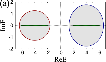
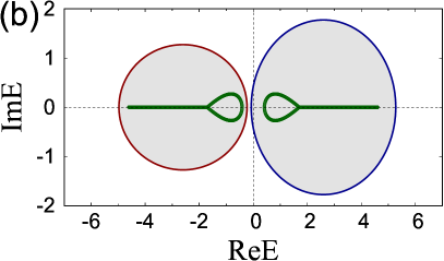
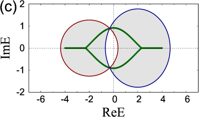
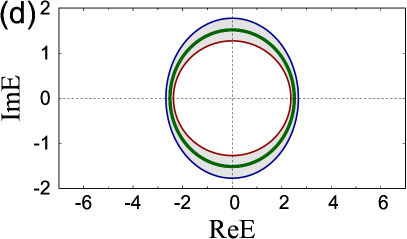
Figure 1: PBC junction spectra (green dots) for different on-site potentials. (a)$\epsilon_{2}=4$, (b)$\epsilon_{2}=2.6$, (c)$\epsilon_{2}=2$ and (d)$\epsilon_{2}=0$ with the condition $\epsilon_{1}=-\epsilon_{2}$. The other parameters are set as $t_{1}=t_{2}=1$, $\gamma_{1}=0.6$, $\gamma_{2}=0.8$ and $N_{1}=N_{2}=500$. PBC spectra for subsystems I and II, $\sigma_{\rm PBC}^{(1)}$ and $\sigma_{\rm PBC}^{(2)}$, are shown by the red and blue ellipses, respectively. The gray regions mean $\Delta w(E_{p})\neq 0$.

Figure 1 shows the spectra for the junction systems with PBC (PBC junction spectra, in short) on the complex plane for different values of on-site potentials. Since $\gamma_{1}$ and $\gamma_{2}$ are set to be positive, $W_{1}=W_{2}=1$. As $\epsilon_{2}$ approaches infinity, each subsystem becomes isolated from each other in the energy space, expected to be independent Hatano-Nelson model, Eq. (1), with OBC. Then, the PBC junction spectrum forms two energy bands on the real axis, which are the same with two spectra of the Hatano-Nelson model with OBC with $\epsilon_{1}$ and $\epsilon_{2}$. The numerical result in Fig. 1(a) agrees with this expectation even at $|\epsilon_{1}-\epsilon_{2}|=8$.

We check how the PBC junction spectrum behaves as we decrease the difference in on-site potential $|\epsilon_{1}-\epsilon_{2}|$. As shown in Fig. 1(b), when the PBC spectra for the subsystems I and II get closer but are not overlapped each other, we see that the PBC junction spectrum forms a loop at the edge of each band (note that this does not imply the inconsistency of the BEC for the point-gap topological phases[46] since the system is subject to PBC.). When $\sigma_{\rm PBC}^{(1)}$ and $\sigma_{\rm PBC}^{(2)}$ begin to intersect, the two loops merge into a single loop passing through the crossing points [Fig. 1(c)]. When the on-site potentials become equal to each other, the PBC junction spectrum becomes an ellipse, similar to the PBC spectrum in Eq. (2), as shown in Fig. 1(d). For all cases, we observe that the PBC junction spectrum $\sigma_{\rm PBC}^{\rm junc}$ appears in the region where $\Delta w\neq 0$, satisfying Eq. (16).

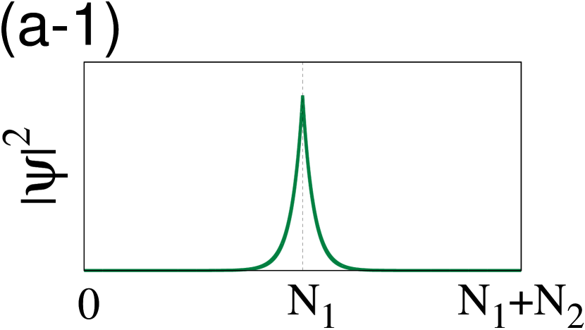
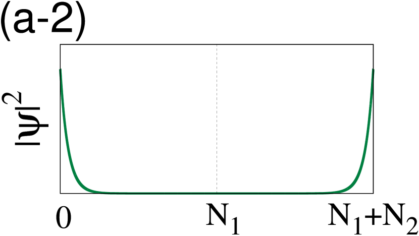
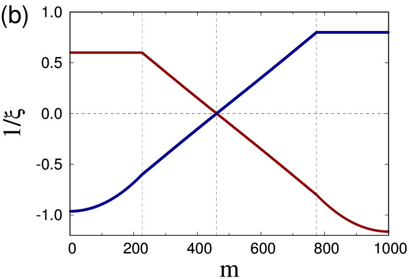
Figure 2: (a): Schematic plots of eigenstates $|\psi_{n}|^{2}$ corresponding to complex eigenenergies appearing inside $\sigma_{\rm PBC}^{(1)}$ [(a-1)] and $\sigma_{\rm PBC}^{(2)}$ [(a-2)] in Fig. 1(c). The eigenstates are localized near the boundary of subsystems. Note that PBC are imposed on both edges. (b): Inverse of the localization lengths $\xi_{i=1}$ (red dots) and $\xi_{i=2}$ (blue dots) in the subsystem I and II, respectively, in the junction system of Fig. 1(c). $m$ is numbered in ascending order of the real part of the eigenenergy values.

Next, we consider the probability distribution function (PDF) of an eigenstate $|\psi_{n}|^{2}$ in junction systems with PBC. We show two PDFs corresponding to the eigenenergies in Fig. 1(c) as typical examples. We see that both PDFs are localized near the boundaries of the subsystems. We remark that the eigenstate in Fig. 2(a-1) [Fig. 2(a-2)] whose eigenenergy is inside the $\sigma_{\rm PBC}^{(1)}$ ($\sigma_{\rm PBC}^{(2)}$) is localized only near $n=N_{1}$ ($n=1$). This can be explained as follows. Since the subsystem ${\rm I}$ dominates the eigenstate in Fig. 2(a-1), the PDF shows the peak near the right edge of the subsystem ${\rm I}$ as the skin effect due to $\gamma_{1}>0$. Meanwhile, for the subsystem ${\rm II}$, the PDF localized near the left edge of the subsystem ${\rm II}$ as the proximity effects of the peak in the subsystem ${\rm I}$. We shall henceforth call this the non-Hermitian proximity effect. The result in Fig. 2(a-2) can be explained in the same way as above.

To study the localization properties further, we calculate the localization length for each subsystem, $\xi_{i=1,2}$, defined as $|\psi_{n}|\propto e^{n/\xi_{i}}$ for $n$ in each subsystem, by numerical fittings. Note that $\xi_{i}$ can take a negative value representing the exponential decay with increasing $n$. Fig. 2(b) shows $1/\xi_{i}$ of all the eigenstates in Fig. 1(c).

First, we consider the eigenenergies on the real axis. We see that $\xi_{1}=1/\gamma_{1}$ for all negative eigenenergies on the real axis, which is consistent with the localization length of an isolated subsystem I with OBC, while the other localization length, $\xi_{2}$, increases gradually as the corresponding eigenenergy decreases ($m\leq 227$). According to our analytic calculations, the localization length $\xi_{2}$ whose eigenenergy is negative infinity as $\epsilon_{1}=-\epsilon_{2}\rightarrow\infty$, eventually converges to zero, which is reasonable by considering the physical meaning. The above analysis can also be applied to all positive eigenenergies on the real axis ($m\geq 774$).

Next, we shift our focus to the complex eigenenergies ($227<m<774$). In this region, $\xi_{1}=-\xi_{2}$ is expected by our analytic results [67] and confirmed numerically in Fig. 2(b). Remarkably, the absolute values of the localization lengths are exactly the same, nevertheless the values of the parameters $\gamma_{i}$ and $\epsilon_{i}$ are different for each subsystem. According to our analytic calculation (Sec. II A in [67]), $|\xi_{1}|=|\xi_{2}|$ remains satisfied even when $t_{1}\neq t_{2}$. This is one of the unique properties of non-Hermitian proximity effects. Further, we concentrate on the eigenenrgies at the intersections of $\sigma_{\rm PBC}^{(1)}$ and $\sigma_{\rm PBC}^{(2)}$ in Fig. 1(c), where the winding number cannot be defined. The localization lengths of the corresponding eigenenergies are shown at $m=460,461$ in Fig. 2(b). Since $1/\xi_{i=1,2}=0$, we find the eigenstates for these two eigenenergies delocalize. This result also agrees with our analytic calculations.

Our investigation confirms that the results for additional cases in Fig. 1 are consistent with our analytic results. We consider that the BEC we established can generally be applied to the point-gap topological phases in junction systems.

Case II: $W_{1}\neq W_{2}$.

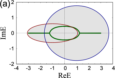
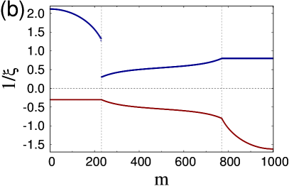
Figure 3: (a): PBC junction spectrum (green dots). All the parameters are the same with Fig, 1(c), but only the value of $\gamma_{1}$ is set as $-0.3$. PBC spectra for subsystems I and II, $\sigma_{\rm PBC}^{(1)}$ and $\sigma_{\rm PBC}^{(2)}$, are shown by the red and blue ellipses, respectively. The gray regions mean $\Delta w\neq 0$. (b): Inverse of the localization lengths $\xi_{i=1}$ (red dots) and $\xi_{i=2}$ (blue dots) in the subsystem I and II, respectively, in the junction system of Fig. 3(a). $m$ is numbered in ascending order of the real part of the eigenenergy values.

Figure 3(a) shows the PBC junction spectrum where $W_{1}=-1$ and $W_{2}=1$. In this case, we see that the spectrum appears even in the internal area shared by $\sigma_{\rm PBC}^{(1)}$ and $\sigma_{\rm PBC}^{(2)}$ while it does not where $W_{1}=W_{2}$ [Fig. 1(c) and (d)]. But this is not a violation of BEC for junction systems with PBC since $\Delta w=2$ for that area. Therefore, Eq. (16) is also confirmed here without exception. Also, the eigenstates, as can be seen in Fig. 3(b), are localized near the boundaries of the subsystems, exhibiting the non-Hermitian proximity effects. The localization lengths in Fig. 3(b) show the same behaviors as the previous case [Fig. 2(b)].

Junction systems with OBC. To clarify of the BEC for the point-gap topological phases in junction systems, hereafter, we consider the junction system with OBC in Eq. (5) with $H_{\text{BC}}=\epsilon_{2}c_{N_{1}+N_{2}}^{\dagger}c_{N_{1}+N_{2}}$. Since OBC is implemented by removing hopping terms between two neighboring sites, there are $N_{1}+N_{2}$ cases for implementing the removal of hopping terms in the model. While, in principle, our analytical method can be applied to the other cases, we focus on the above $H_{\text{BC}}$ for the present analytical calculation.

The eigenfunction can be approximated as (see Ref. [67])

$$\left|\psi_{n}\right|\propto\left\{\begin{array}[]{ll}\exp[(\gamma_{1}+l_{1})n]&\quad(n\in[1,N_{1}]),\\ \exp[(\gamma_{2}-l_{2})n]&\quad(n\in[N_{1}+1,N_{1}+N_{2}]).\end{array}\right.$$ (23)

We find that there is no solution where $l_{1},l_{2}>0$. This means that the spectrum for the junction system with OBC must appear on the real axis, particularly on the OBC spectra for each subsystem.

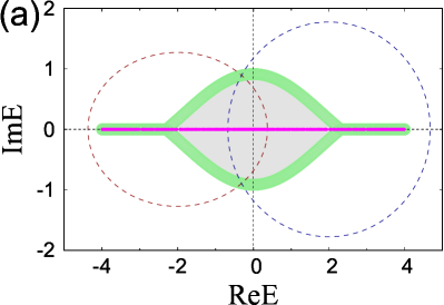
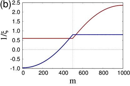
Figure 4: (a): Spectra (magenta dots) of the junction system with all possible OBC ($N_{1}+N_{2}$ cases). All the parameters are the same with Fig, 1(c) except for the system size ($N_{1}=N_{2}=30$). PBC spectra for subsystems I and II, $\sigma_{\rm PBC}^{(1)}$ and $\sigma_{\rm PBC}^{(2)}$, are shown by the red and blue ellipses, respectively. The PBC junction spectrum is shown by the green dots and the gray region means $w^{\rm junc}\neq 0$. (b): Inverse of the localization lengths $\xi_{i=1}$ (red dots) and $\xi_{i=2}$ (blue dots) in the subsystem I and II, respectively, in the junction system with OBC. All the parameters are the same with Fig. 1(c). $m$ is numbered in ascending order of the real part of the eigenenergy values.

Figure 4(a) shows the spectra for the junction system with all possible OBC calculated numerically. As discussed above, we numerically confirm that all the spectra appear on the real axis. Further, regardless of the removal position, it can be numerically confirmed and analytically explained that all spectra appear on and inside $\sigma_{\rm PBC}^{\rm junc}$ without exception. Actually, the winding number of the junction system $w^{\rm junc}(E_{p})$ which is not well defined by Eq. (3) is estimated to be unity since a Hamiltonian connected by the continuous deformation of $t_{1}=t_{2}$ and $\gamma_{1}=\gamma_{2}>0$ without closing the point gap gives $w(E_{p})=1$ from Eq. (3), where $E_{p}$ locates in the point gap. Thus, we confirm that the spectrum for the junction system with OBC (OBC junction spectrum, in short) appears on and inside the spectrum for the corresponding junction system with PBC regardless of the removal position for hopping terms. This result is consistent with the BEC for the point-gap topological phases[46].

Figure 4(b) shows the localization properties of the junction system with OBC which is implemented by removing the hopping terms between $n=1$ and $n=N_{1}+N_{2}$. We see that $\xi_{1}=1/\gamma_{1}$ ($\xi_{2}=1/\gamma_{2}$) for all the eigenenergies on the OBC spectrum for the subsystem ${\rm I}$ (${\rm II}$), which is also consistent with localization length of an isolated subsystem ${\rm I}$ (${\rm II}$). In contrast to the previous arguments on Figs. 2(b) and 3(b), we see that both $\xi_{1}$ and $\xi_{2}$ are positive for $m\geq 367$, meaning the correspponding PDFs show the peak only at the right edge of the whole system, not exhibiting the non-Hermitian proximity effects. This result is reasonable because of the absence of the hopping between $n=1$ and $N_{1}+N_{2}$ and $\gamma_{1},\gamma_{2}>0$. For the eigenenergies whose eigenstates are dominated by the subsystem ${\rm I}$ ($m\leq 366$), however, we find the non-Hermitian proximity effects even in the junction system with OBC.

Conclusion. In this Letter, we have established the BEC for the point-gap topological phases in junction systems. To summarize, for the point-gap topological phases in junction systems with PBC, the PBC junction spectra do not appear where the winding number for each subsystem is equal. Further, almost all the eigenstates are localized near the interface and exhibit the non-Hermitian proximity effects. We also revealed that the OBC junction spectrum appears on and inside the corresponding PBC junction spectrum. Thereby, the BEC for the point-gap topological phases [21, 46, 47] can be applied to the junction systems with OBC as well.

Since the BEC for junction systems in Hermitian systems requiring that the number of edge states is given by the difference in topological number for each subsystem is generally valid, the BEC for non-Hermitian junction systems we established, Eqs. (16) and (17), is regarded as a natural extension of the BEC for Hermitian junction systems. Therefore, while our conclusion is derived from a specific lattice model, we consider that the present statements can be applied to more general junction systems with point-gap topological phases. Especially, it is quite interesting to study the non-Hermitian proximity effects for other systems.

We thank Yasuhiro Asano, Masatoshi Sato, and Kousuke Yakubo for helpful discussions. This work was supported by KAKENHI (Grants No. JP19H00658, No. JP20H01828, No. JP21H01005, No. JP22K03463 and No. JP22H01140).

References

- Hatano and Nelson [1996] N. Hatano and D. R. Nelson, Phys. Rev. Lett. 77, 570 (1996).
- Hatano and Nelson [1997] N. Hatano and D. R. Nelson, Phys. Rev. B 56, 8651 (1997).
- Hatano and Nelson [1998] N. Hatano and D. R. Nelson, Phys. Rev. B 58, 8384 (1998).
- Bender and Boettcher [1998] C. M. Bender and S. Boettcher, Phys. Rev. Lett. 80, 5243 (1998).
- Bender et al. [2002] C. M. Bender, D. C. Brody, and H. F. Jones, Phys. Rev. Lett. 89, 270401 (2002).
- Rudner and Levitov [2009] M. S. Rudner and L. S. Levitov, Phys. Rev. Lett. 102, 065703 (2009).
- Esaki et al. [2011] K. Esaki, M. Sato, K. Hasebe, and M. Kohmoto, Phys. Rev. B 84, 205128 (2011).
- Hu and Hughes [2011] Y. C. Hu and T. L. Hughes, Phys. Rev. B 84, 153101 (2011).
- Lee and Chan [2014] T. E. Lee and C.-K. Chan, Phys. Rev. X 4, 041001 (2014).
- Lee et al. [2014] T. E. Lee, F. Reiter, and N. Moiseyev, Phys. Rev. Lett. 113, 250401 (2014).
- Lee [2016] T. E. Lee, Phys. Rev. Lett. 116, 133903 (2016).
- Mochizuki et al. [2016] K. Mochizuki, D. Kim, and H. Obuse, Phys. Rev. A 93, 062116 (2016).
- González and Molina [2017] J. González and R. A. Molina, Phys. Rev. B 96, 045437 (2017).
- Leykam et al. [2017] D. Leykam, K. Y. Bliokh, C. Huang, Y. D. Chong, and F. Nori, Phys. Rev. Lett. 118, 040401 (2017).
- Xiao et al. [2017] L. Xiao, X. Zhan, Z. H. Bian, K. K. Wang, X. Zhang, X. P. Wang, J. Li, K. Mochizuki, D. Kim, N. Kawakami, W. Yi, H. Obuse, B. C. Sanders, and P. Xue, Nat. Phys. 13, 1117 (2017).
- Kawabata et al. [2018] K. Kawabata, Y. Ashida, H. Katsura, and M. Ueda, Phys. Rev. B 98, 085116 (2018).
- Wang et al. [2018] M. Wang, L. Ye, J. Christensen, and Z. Liu, Phys. Rev. Lett. 120, 246601 (2018).
- Nakagawa et al. [2018] M. Nakagawa, N. Kawakami, and M. Ueda, Phys. Rev. Lett. 121, 203001 (2018).
- Yao and Wang [2018] S. Yao and Z. Wang, Phys. Rev. Lett. 121, 086803 (2018).
- Yao et al. [2018] S. Yao, F. Song, and Z. Wang, Phys. Rev. Lett. 121, 136802 (2018).
- Gong et al. [2018] Z. Gong, Y. Ashida, K. Kawabata, K. Takasan, S. Higashikawa, and M. Ueda, Phys. Rev. X 8, 031079 (2018).
- Lieu [2018] S. Lieu, Phys. Rev. B 97, 045106 (2018).
- Zyuzin and Zyuzin [2018] A. A. Zyuzin and A. Y. Zyuzin, Phys. Rev. B 97, 041203(R) (2018).
- Yoshida et al. [2018] T. Yoshida, R. Peters, and N. Kawakami, Phys. Rev. B 98, 035141 (2018).
- Chen and Zhai [2018] Y. Chen and H. Zhai, Phys. Rev. B 98, 245130 (2018).
- Shen and Fu [2018] H. Shen and L. Fu, Phys. Rev. Lett. 121, 026403 (2018).
- Molina and González [2018] R. A. Molina and J. González, Phys. Rev. Lett. 120, 146601 (2018).
- Takata and Notomi [2018] K. Takata and M. Notomi, Phys. Rev. Lett. 121, 213902 (2018).
- Zhou and Gong [2018] L. Zhou and J. Gong, Phys. Rev. B 98, 205417 (2018).
- Zhou et al. [2018] L. Zhou, Q.-h. Wang, H. Wang, and J. Gong, Phys. Rev. A 98, 022129 (2018).
- Kawabata et al. [2019] K. Kawabata, K. Shiozaki, M. Ueda, and M. Sato, Phys. Rev. X 9, 041015 (2019).
- Yokomizo and Murakami [2019] K. Yokomizo and S. Murakami, Phys. Rev. Lett. 123, 066404 (2019).
- Imura and Takane [2019] K.-I. Imura and Y. Takane, Phys. Rev. B 100, 165430 (2019).
- Liu et al. [2019] T. Liu, Y.-R. Zhang, Q. Ai, Z. Gong, K. Kawabata, M. Ueda, and F. Nori, Phys. Rev. Lett. 122, 076801 (2019).
- Yamamoto et al. [2019] K. Yamamoto, M. Nakagawa, K. Adachi, K. Takasan, M. Ueda, and N. Kawakami, Phys. Rev. Lett. 123, 123601 (2019).
- Xiao et al. [2019] L. Xiao, K. Wang, X. Zhan, Z. Bian, K. Kawabata, M. Ueda, W. Yi, and P. Xue, Phys. Rev. Lett. 123, 230401 (2019).
- Li et al. [2019] J. Li, A. K. Harter, J. Liu, L. de Melo, Y. N. Joglekar, and L. Luo, Nat. Commun. 10, 855 (2019).
- Ezawa [2019] M. Ezawa, Phys. Rev. B 99, 121411(R) (2019).
- Okugawa and Yokoyama [2019] R. Okugawa and T. Yokoyama, Phys. Rev. B 99, 041202(R) (2019).
- Budich et al. [2019] J. C. Budich, J. Carlström, F. K. Kunst, and E. J. Bergholtz, Phys. Rev. B 99, 041406(R) (2019).
- Yang and Hu [2019] Z. Yang and J. Hu, Phys. Rev. B 99, 081102(R) (2019).
- Yoshida et al. [2019] T. Yoshida, R. Peters, N. Kawakami, and Y. Hatsugai, Phys. Rev. B 99, 121101(R) (2019).
- Wu et al. [2019] Y. Wu, W. Liu, J. Geng, X. Song, X. Ye, C.-K. Duan, X. Rong, and J. Du, Science 364, 878 (2019).
- Ashida et al. [2020] Y. Ashida, Z. Gong, and M. Ueda, Advances in Physics 69, 249 (2020).
- Borgnia et al. [2020] D. S. Borgnia, A. J. Kruchkov, and R.-J. Slager, Phys. Rev. Lett. 124, 056802 (2020).
- Okuma et al. [2020] N. Okuma, K. Kawabata, K. Shiozaki, and M. Sato, Phys. Rev. Lett. 124, 086801 (2020).
- Zhang et al. [2020] K. Zhang, Z. Yang, and C. Fang, Phys. Rev. Lett. 125, 126402 (2020).
- Weidemann et al. [2020] S. Weidemann, M. Kremer, T. Helbig, T. Hofmann, A. Stegmaier, M. Greiter, R. Thomale, and A. Szameit, Science 368, 311 (2020), https://www.science.org/doi/pdf/10.1126/science.aaz8727 .
- Xiao et al. [2020] L. Xiao, T. Deng, K. Wang, G. Zhu, Z. Wang, W. Yi, and P. Xue, Nature Physics 16, 761 (2020).
- Bergholtz et al. [2021] E. J. Bergholtz, J. C. Budich, and F. K. Kunst, Rev. Mod. Phys. 93, 015005 (2021).
- Hatano and Obuse [2021] N. Hatano and H. Obuse, Annals of Physics 435, 168615 (2021).
- Longhi [2021] S. Longhi, Opt. Lett. 46, 6107 (2021).
- [53] S. Weidemann, M. Kremer, S. Longhi, and A. Szameit, Nature , 354.
- Kawasaki et al. [2022] M. Kawasaki, K. Mochizuki, and H. Obuse, Phys. Rev. B 106, 035408 (2022).
- Okuma and Sato [2023] N. Okuma and M. Sato, Annual Review of Condensed Matter Physics 14, 83 (2023).
- Schindler et al. [2023] F. Schindler, K. Gu, B. Lian, and K. Kawabata, PRX Quantum 4, 030315 (2023).
- Makris et al. [2008] K. G. Makris, R. El-Ganainy, D. N. Christodoulides, and Z. H. Musslimani, Phys. Rev. Lett. 100, 103904 (2008).
- Klaiman et al. [2008] S. Klaiman, U. Günther, and N. Moiseyev, Phys. Rev. Lett. 101, 080402 (2008).
- Guo et al. [2009] A. Guo, G. J. Salamo, D. Duchesne, R. Morandotti, M. Volatier-Ravat, V. Aimez, G. A. Siviloglou, and D. N. Christodoulides, Phys. Rev. Lett. 103, 093902 (2009).
- Rüter et al. [2010] C. E. Rüter, K. G. Makris, R. El-Ganainy, D. N. Christodoulides, M. Segev, and D. Kip, Nat. Phys. 6, 192 (2010).
- Feng et al. [2013] L. Feng, Y.-L. Xu, W. S. Fegadolli, M.-H. Lu, J. E. B. Oliveira, V. R. Almeida, Y.-F. Chen, and A. Scherer, Nat. Mater. 12, 108 (2013).
- Zeuner et al. [2015] J. M. Zeuner, M. C. Rechtsman, Y. Plotnik, Y. Lumer, S. Nolte, M. S. Rudner, M. Segev, and A. Szameit, Phys. Rev. Lett. 115, 040402 (2015).
- Malzard et al. [2015] S. Malzard, C. Poli, and H. Schomerus, Phys. Rev. Lett. 115, 200402 (2015).
- Rosenthal et al. [2018] E. I. Rosenthal, N. K. Ehrlich, M. S. Rudner, A. P. Higginbotham, and K. W. Lehnert, Phys. Rev. B 97, 220301(R) (2018).
- Parto et al. [2018] M. Parto, S. Wittek, H. Hodaei, G. Harari, M. A. Bandres, J. Ren, M. C. Rechtsman, M. Segev, D. N. Christodoulides, and M. Khajavikhan, Phys. Rev. Lett. 120, 113901 (2018).
- Malzard and Schomerus [2018] S. Malzard and H. Schomerus, Phys. Rev. A 98, 033807 (2018).
- [67] See the Summpelemtal Material for details .