Intra-atomic Hund’s exchange interaction determines spin states and energetics of Li-rich layered sulfides for battery applications

Abstract

Motivated by experimental suggestions of anionic redox processes helping to design higher energy lithium ion-battery cathode materials, we investigate this effect using first-principles electronic structure calculations for Li-rich layered sulfides. We identify the determination of the energetic contribution of intra-atomic Hund’s exchange coupling as a major obstacle to a reliable theoretical description. We overcome this challenge by developing a particularly efficient flavor of charge-self-consistent combined density functional + dynamical mean-field theory (DFT+DMFT) calculations. Our scheme allows us to describe the spin ground states of the transition metal $d$ shell, the electronic structure of the materials, and its energetics. As a result of the high-spin to low-spin transition the average intercalation voltage shows intriguing non-monotonic behavior. We rationalize these findings by an analysis of the fluctuations of spin and charge degrees of freedom. Our work demonstrates the relevance of most recent insights into correlated electron materials for the physics of functional materials such as Li-ion battery compounds.

I Introduction

Many modern technologies such as mobile devices or electric cars hinge upon the development of high-energy density batteries. Finding cathode materials fulfilling the mandatory criteria of being safe and inexpensive with high capacity and intercalation voltage is a bottleneck in the field. A traditional, extensively studied and commercially successful example is LiCoO₂ Mizushima et al. (1980). While for many years, the main strategy for cathode materials in Li-ion batteries purely relied on cationic redox, lithium-rich layered manganese oxides have recently attracted great interest, involving both cationic and anionic redox processes Lu et al. (2001); Assat and Tarascon (2018); Li and Xia (2017). The lithium-rich layered manganese oxide Li₂MnO₃ is the parent compound of the currently used Li[Li_xMn_yNi_zCo_1-x-y-z]O₂, which are famous for their reversible high capacities exceeding 250 mAh/g Li and Xia (2017); Assat and Tarascon (2018); Thackeray et al. (2007). Undesired consequences of anionic redox processes are, however, potential capacity loss and structural degradation, as well as hysteresis.

Recently, new Li-rich layered sulfides Li_x[Li_0.33-2y/3Ti_0.67-y/3Fe_y]S₂ have been reported Saha et al. (2019). Its negligible cycle irreversibility, mitigated voltage fade upon long cycling, low voltage hysteresis, and fast kinetics suggest a new direction to alleviate the practical limitations of using the anionic redox mechanism. Motivated by their experimental realization, we perform first-principles calculations for the above-mentioned Li-rich layered sulfides, using as prototypes the fully lithiated and delithiated materials. We focus on the $y=1/3$ case, i.e., Li_x+0.11Ti_0.56Fe_0.33S₂ (LTFS_x). Note that the value $y=1/3$ is close to the optimal value reported in experiment, namely $y=0.3$ Saha et al. (2019).

First-principles electronic structure calculations based on density functional theory (DFT) within the local density approximation (LDA) and generalized gradient approximation (GGA) have developed into a tremendously useful tool for addressing materials properties and even helping design functional materials. Nevertheless, these approximations have known limitations in describing materials containing open $d$- or $f$-shells with sizable Coulomb interactions. Indeed, the standard LDA/GGA description based on the delocalized electron gas picture is not an optimal starting point for the rather localized behavior of $d$- or $f$-electrons. In the materials of interest here, as we will see below, a particular challenge is the necessity of capturing the spin-state of these localized electrons correctly, since the energetics of the materials depend on the corresponding exchange contribution. A second limitation arises for properties that involve excited states, which are in principle inaccessible to standard DFT, even if the exact ground state energy functional was available. Over the last decades, combinations of LDA/GGA with many-body techniques have evolved into extremely useful and well-established tools overcoming these limitations. Among these, DFT plus dynamical mean-field theory (DFT+DMFT) Metzner and Vollhardt (1989); Georges and Kotliar (1992); Zhang et al. (1993); Anisimov et al. (1997); Lichtenstein and Katsnelson (1998) and DFT$+U$ Anisimov et al. (1991); Liechtenstein et al. (1995) stand out as methods of choice.

Here, we suggest a new flavor of the charge-self-consistency in DFT+DMFT methods, to describe the observed electronic ground states and the competing phases of our target materials, namely a high-spin (HS) Mott insulator, a correlated metal, and a low-spin (LS) band insulator phase. We show that the energetics of the cathode materials largely depends on the spin ground state, revealing that the impact of the Hund’s coupling is not only of theoretical interest but has practical implications for battery materials. These findings place our target materials in the context of the nowadays celebrated “Hund’s materials”, where intra-atomic exchange amplifies the consequences of strong local Coulomb interactions de’ Medici et al. (2011); Georges et al. (2013). They should be viewed as strongly correlated electron systems, the properties of which can be described in the language of modern first-principles many-body techniques.

The paper is organized as follows. In Sec. II, we present details of our calculational techniques. In particular, we have developed a new flavor for DFT+DMFT that takes into account charge redistributions due to correlation effects. In Sec. III, the results of our calculations are presented and comparisons between static (DFT$+U$) and dynamic (DFT+DMFT) mean field approximations to electronic Coulomb correlations are made. Finally, a summary and some conclusions are given in Sec. IV.

II Methods and formalism: charge-self-consistent DMFT scheme

Within the DFT+DMFT framework, the charge-density $\rho(r)$ and the local Green’s function $G_{\rm loc}(i\omega_{n})$ are determined by the stationary condition of the free energy functional $\Gamma[\rho,G_{\rm loc}]$ Georges et al. (1996). Single-shot (i.e. non-charge-self-consistent) DFT+DMFT calculations are performed in many works in the literature, where $\rho$ is given from LDA/GGA calculations. In the case of the LTFS, however, due to the larger covalency between S-$p$ and Fe-$d$ compared to oxides, it is important to take into account the effect of the charge redistribution due to correlation effects. The importance of the charge redistribution is demonstrated by the fact that conventional one-shot DFT+DMFT with fixed DFT charge density predicts a significantly underestimated voltage as we will discuss in Sec. III. On the other hand, given the large unit cells with low symmetry, fully charge-self-consistent DFT+DMFT calculations are hardly accessible due to the computational cost.

In this paper, we use an efficient way to calculate the total energy given as

$$E_{{\rm DFT}+{\rm DMFT}}= E_{{\rm GGA}}[\rho_{U}]-\braket{H_{{\rm KS}}^{GGA}[\rho_{U}]}_{\rho_{U}}+\operatorname{Tr}(H_{{\rm KS}}[\rho_{U}]G)$$

$$+\frac{1}{2}\operatorname{Tr}\Sigma G-E_{{\rm DC}}^{{\rm FLLnS}},$$ (1)

where the GGA energy functional $E_{{\rm GGA}}[\rho_{U}]$ and $H_{KS}^{GGA}[\rho_{U}]=\frac{\delta E_{{\rm GGA}}}{\delta\rho(r)}\bigr{|}_{\rho=\rho_{U}}$ are evaluated at the ground state density $\rho_{U}(r)$ obtained from GGA$+U$ calculations. The double counting $E_{{\rm DC}}^{{\rm FLLnS}}$ is taken to be the spin-independent "fully localized limit" double counting using the spin-averaged occupations Anisimov et al. (1993), dubbed "FLL-nS" in Ref. Ylvisaker et al. (2009).

We stress that $\rho_{U}$ differs from the ground state density $\rho_{0}$ of $H_{{\rm KS}}[\rho_{U}]$ due to the absence of the $+U$ contribution in $E_{{\rm GGA}}$ and $H_{KS}^{GGA}$. One can understand our scheme as follows: i) First, charge-self-consistent DFT+DMFT calculations are performed with a Hartree-Fock impurity solver. ii) Given the resulting charge density, we produce the Hamiltonian $H_{{\rm HK}}+H_{{\rm int}}$ on which the DMFT calculations are performed with a more sophisticated impurity solver, namely continuous-time quantum Monte Carlo (CT-QMC) simulations Werner et al. (2006); Werner and Millis (2006). This approach is not only computationally efficient, but also useful for comparing the results to the DFT$+U$ calculations. Because both DFT$+U$ and +DMFT use the same charge density $\rho_{U}$, it is easier to investigate the correction stemming from the dynamical self-energy, without ambiguity. Once we use the HF solver in step ii), for example, $E_{{\rm DFT+DMFT}}$ exactly reduces to the DFT$+U$ results.

In Eq. (1), we have a adopted charge-only-dependent exchange-correlation GGA functional and FLL-nS double counting. The FLL-nS double counting scheme has been introduced within the DFT$+U$ functional Ylvisaker et al. (2009) (cFLL in the notation of Ref. Ryee and Han, 2018):

$$E_{{\rm DFT}+U}[\rho_{U}]=E_{{\rm DFT}}[\rho_{U}]+E_{{\rm int}}^{U}[n_{\alpha\beta}^{\sigma}]-E_{{\rm DC}}^{{\rm FLLnS}}[N_{d}],$$ (2)

where $E_{{\rm int}}^{U}$, and $E_{{\rm DC}}^{{\rm FLLnS}}$ are the Hartree-Fock energy of the local Coulomb interaction, and the double counting contribution, respectively. We note that the $E_{{\rm GGA}}$ and $E_{{\rm DC}}^{{\rm FLLnS}}$ contributions to the total energy depend only on the charge density $\rho=\rho_{\uparrow}+\rho_{\downarrow}$ and the occupation of the $d$-shell $N_{d}=\sum_{\sigma,\alpha}n_{\alpha\alpha}^{\sigma}$ , respectively. The spin density contributions to the total energy are controlled solely by the interaction term $E^{U}_{{\rm int}}$ or by the self-energy $\Sigma^{\sigma}$ in the DMFT formalism. For more details, see Appendix B.

Benchmarks of different DFT$+U$ formalisms Anisimov et al. (1991, 1993); Dudarev et al. (1998); Liechtenstein et al. (1995) have been performed in previous studies Ylvisaker et al. (2009); Ryee and Han (2018). The spin-dependent DFT$+U$ extensions exhibit seemingly unphysical behavior, including an unreasonable $J$ dependence of structural parameters in nickelates Pavarini (2011) and the energy difference between high-spin/low-spin states in 3$d$ and 4$d$ transition-metal compounds Ryee and Han (2018). Similar arguments were also given in the DFT+DMFT context Chen et al. (2015); Park et al. (2014); Chen and Millis (2016).

III Results and discussion

III.1 Electronic structure of the layered sulfides within GGA and GGA$+U$

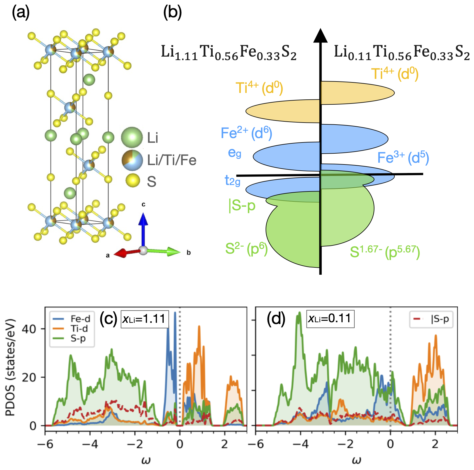
Figure 1: (a) Crystal structure of Li_x[Li_0.33-2y/3Ti_0.67-y/3Fe_y]S₂. Green, blue, and yellow spheres represent Li ions, a mixture of Li/Ti/Fe ions, and S ions, respectively. Visualization was conducted using VESTA Momma and Izumi (2011) (b) Schematic electronic structure near the Fermi level for the $y=1/3$ case. |S-p denotes non-bonding S $3p$ states. The oxidation states are estimated from simple charge counting. (c, d) The projected density of states (PDOS) obtained from GGA calculations. Red dashed lines represent the S $3p$ contained in the octahedron with Li as a central atom, capturing the non-bonding states.

The Li-rich layered Li_1.33-2y/3Ti_0.67-y/3Fe_yS₂ can be thought of as a Li_1.33Ti_0.67S₂ compound, where some of the Ti⁴⁺ have been substituted by Fe²⁺ with a charge compensation by adjusting the Li content. The crystal structure is shown in Fig. 1(a) Saha et al. (2019). It consists of stacks of transition metal disulfide layers crystallizing in a honeycomb lattice structure. Upon lithiation, Li-ions intercalate in the interlayer space or within the layers. At the DFT level, the Fermi surface is dominated by Fe²⁺ $d$-derived bands, which are strongly hybridized with S^2- $p$ orbitals. The Ti⁴⁺ ions are electronically inactive because of their $3d^{0}$ configuration. Upon removal of Li, both cationic Fe²⁺ and anionic S^2- contribute to the corresponding redox processes Saha et al. (2019). As shown in Ref. Saha et al., 2019, the experimentally observed capacity of 245 mAhg^-1 for Li_1.13Ti_0.57 Fe_0.3S₂ ($y=0.3$), which corresponds to the removal of $\sim 1.06$ Li ions per formula unit, cannot be reached by cationic redox alone, even when assuming a multi-electron oxidation from Fe²⁺ to Fe⁴⁺. Hence anionic redox processes, leaving unoccupied sulfur $p$ states near the Fermi level in Fig. 1(d), have to be invoked to understand the high capacity of these materials. From a simple charge count, we can estimate the oxidation states Fe³⁺ ($d^{5}$) and S^1.67- ($p^{5.67}$) for fully charged (i.e., fully oxidized) LTFS₀ (see Fig. 1(b)).

Fig. 1(c) and (d) show the projected density of states (PDOS) corresponding to the non-spin-polarized Kohn-Sham band structure obtained from GGA calculations. Within the GGA, fully discharged LTFS₁ is a band insulator with fully occupied $t_{2g}$ orbitals, while LTFS₀ is metallic with nominal $t_{2g}^{5}e_{g}^{0}$ configuration. Although the FeS₆ octahedra are slightly distorted due to the different size of the Li, Ti, and Fe ions in the metal layer, we will refer to the three lower-lying orbitals as $t_{2g}$ and to the two higher-lying ones as $e_{g}$. Due to the large hybridization between the Fe-$d$ and S-$p$ states in LTFS₀, larger ligand field splittings are expected from different hopping strengths for $t_{2g}$ and $e_{g}$ orbitals. To calculate the ligand field splittings, projective Wannier functions within an energy window of $W=[-1,3]$ eV were constructed. The on-site energy level differences between the three lower- and two higher-lying orbitals, denoting the crystal-field splitting, amount to 1.04 eV and 1.78 eV for LTFS₁ and LTFS₀, respectively. Here the smaller crystal-field splitting for LTFS₁ compared to LTFS₀ also implies a redox-driven spin-state transition and is consistent with the experimentally observed high-spin and low-spin states for LTFS₁ and LTFS₀, respectively Watanabe et al. (2019); Saha et al. (2019).

The red dashed lines in Fig. 1 (c, d) represent the S $3p$ states of the S atoms forming the LiS₆ octahedra, which are of non-bonding nature. We calculated $r_{nb}$, the fraction of the partial charge residing in the “non-bonding” state by integrating the relevant partial DOS (red dashed and solid green lines) shown in Fig. 1 (c) and (d) within a given energy window. For LTFS₁, $r_{nb}$ is 0.80 in the energy window $[-2,0]$, while 0.46 for $[-6,-2]$. The larger $r_{nb}$ near the Fermi level clearly shows the non-bonding contribution in the above bonding states as presented in Fig. 1(b).

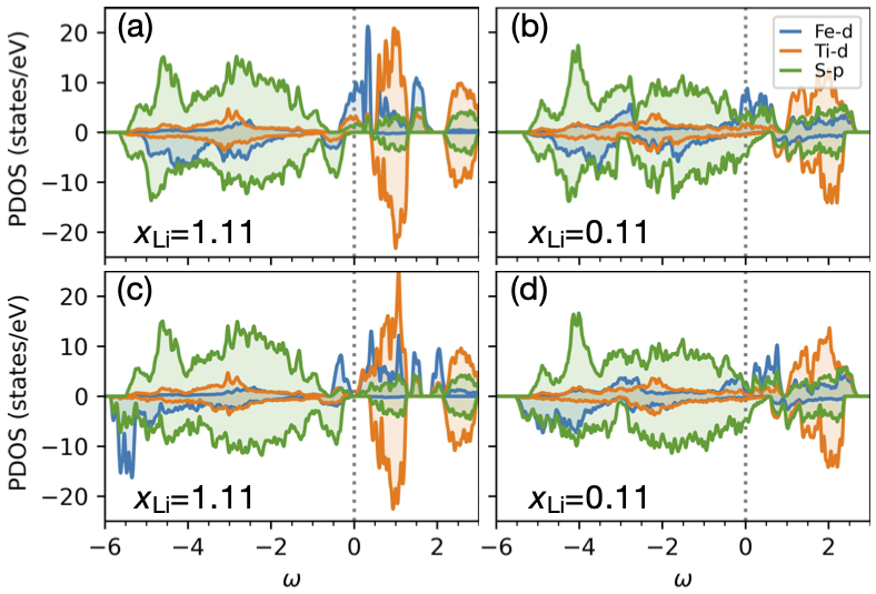
Figure 2: The projected density of states (PDOS) calculated from (a,b) spin-polarized GGA (SGGA), and (c, d) GGA$+U$. The upper and lower panels in the PDOS plots represent up and down spin components, respectively.

Fig. 2(a) and (b) present the PDOS with spin-polarized GGA (SGGA). LTFS₁ is metallic with HS Fe-$d$ configuration, while the Fe-$d$ shell in the LTFS₀ is not fully polarized with partially unoccupied minority spin components. The spin-configuration is consistent with the previously reported assignments based on Mössbauer spectroscopy experiments, where the fitted spectra show finite quadrupole splitting for both Fe³⁺ and Fe²⁺ oxidation states Saha et al. (2019). Interestingly, when creating a hypothetical oxide compound by replacing S by O, one can artificially tune the ligand splitting due to the corresponding smaller overlap between O-$p$ and Fe-$d$ orbitals as compared to the one of S-$p$ and Fe-$d$ (not shown). The result is a HS configuration for both end-member compounds with large spin magnetic moments on the Fe sites, $M_{s}=3.80$ and $3.49$ $\mu_{B}$, respectively. The appearance of these different spin configurations implies that a change of the anion from O to S can significantly affect battery properties such as the capacity and more so the operating voltageSaha et al. (2019); Watanabe et al. (2019).

The GGA$+U$ results for LTFS₁ and LTFS₀ are shown in Fig. 2(c, d), respectively. The effect of the Coulomb interaction between the localized $d$-electrons is clearly seen from the Mott insulating gap for LTFS₁ and from the suppression of the Fe-$d$ contribution near the Fermi-level. Here, the insulating gap opening is driven by a reduction in the occupancy fluctuations over the three non-degenerate low-lying orbitals, referred to as $t_{2g}$ for convenience, due to the energy penalty of the $\frac{1}{2}(U-J)\sum_{\alpha\sigma}(n_{\alpha\sigma}-n_{\alpha\sigma}^{2})$ term in $\Delta E^{U}$ (See Appendix B). From the SGGA calculation, for example, the eigenvalues of the density matrix for the $t_{2g}$ subspace of the minority spin component are given as 0.27, 0.30, and 0.57, while GGA$+U$ provides 0.26, 0.25, and 0.83. For LTFS₀, however, the spin magnetic moments, $M_{S}=2.30\>\mu_{B}$ are enhanced from the result of GGA, $M_{S}=1.84\>\mu_{B}$, due to the $-\frac{J}{4}M_{S}^{2}$ contribution in $\Delta E^{U}$. Considering the experimental assignment of the LS state to Fe${}^{3+}(d^{5})$ ions in the fully charged sample and the ideal magnetic moments $\sim 1$ $\mu_{B}$ of the $d^{5}$ in the LS state Saha et al. (2019), the predicted magnetic moments by the DFT+$U$ calculations are significantly overestimated, stressing the limitations of the static mean field approximation done in GGA+$U$. This motivated us to go beyond GGA+$U$ and perform GGA+DMFT calculations for these same materials. Detailed comparisons are presented in the next section.

III.2 Electronic structure of the layered sulfides within GGA+DMFT

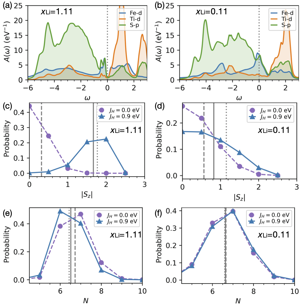
Figure 3: (a, b) The spectral function from GGA+DMFT. Probability of the atomic states in Fe-$d$ shell projected onto the (c, d) spin $S_{z}$ and (e, f) number of electrons $N$. The solid and dashed vertical lines indicate the averaged value for $J_{H}=0.9$ and $0.0$ eV, within GGA+DMFT and the dotted line from the GGA$+U$ calculations.

To capture the electronic ground state or quasi-particle electronic structure of the HS Mott insulating LTFS₁ and the LS correlated metallic LTFS₀, in this section, we have employed GGA+DMFT. Specifically, we study the effect of dynamic correlations between the Fe-$d$ electrons on the electronic structure and the magnetic properties using the Hubbard interaction $U$ and the Hund’s exchange coupling $J_{H}$ as parameters. The paramagnetic GGA+DMFT calculations are performed at an inverse temperature of $\beta=40$ eV^-1 corresponding to about 290 K. Since the occupied valence orbitals are drastically modulated by spin-state transition, the correlation between spin states and redox properties is expected.

In Fig. 3(a) and (b), we present orbital-resolved spectral functions from paramagnetic GGA+DMFT calculations. The difference of these results to the DOS from the static GGA$+U$ approximation is significant, in particular for LTFS₀ near the Fermi-level, underlining the importance of the dynamic correlation effects. Within GGA$+U$, the Fe-$d$ contribution to the DOS near the Fermi level is small, contrasting to the large Fe-$d$ character in the GGA+DMFT result. The suppression of the Fe-$d$ contribution in the GGA$+U$ calculation originates from the suppression of charge fluctuations by the Coulomb interactions (see energy penalty term $\Delta E^{U}$ in Appendix B), favoring integer occupation.

The reason why GGA$+U$ struggles to capture the electronic structure of the correlated metallic phase can be traced back to the absence of dynamical fluctuations in this method. This can be seen from the probability distribution of the atomic configurations. Indeed, solving the DMFT by Monte Carlo sampling has the advantage to give direct access to the charge and spin fluctuations: Fig. 3(c-f) shows the probabilities of the different atomic configurations in terms of the magnitude of the spin component and the orbital occupancies. As expected, a sharp peak at around $\lvert S_{z}\rvert=2$ is observed in Fig. 3(c) indicating the HS configuration. For metallic LTFS₀, the spin fluctuations $\delta\braket{}{S_{z}}{}^{2}=0.33$ with mean value of spin magnetic moments $\braket{\lvert S_{z}\rvert}_{{\rm DMFT}}=0.82$ are lager than that of LTFS₁ ($\delta\braket{}{S_{z}}{}^{2}=0.15$ and $\braket{\lvert S_{z}\rvert}_{{\rm DMFT}}=1.67$). We note that these fluctuations of the spin magnetic moments on the Fe sites cannot be captured in a static-mean-field theory such as DFT+$U$. The calculated magnetic moments in metallic LTFS₀ compounds, $M_{S}=2\braket{\lvert S_{z}\rvert}_{\rm DMFT}\sim 1.65$ $\mu_{B}$, are in better agreement with the experimental assignment of the LS state Saha et al. (2019) than GGA+$U$ (2.30 $\mu_{B}$).

The probability distribution projected onto the number of electrons is also presented in Fig. 3(e, f). Both compounds show non-negligible charge fluctuations with $\delta\braket{N}^{2}=0.48$ and $0.93$ for LTFS₁ and LTFS₀, respectively. As expected, the metallic LTFS₀ shows larger fluctuations than insulating LTFS₁. Due to the strong hybridization with the S-$p$ orbitals the mean occupation is slightly larger than nominally expected. In particular, the electron occupancy of 6.63 of the Fe-$d$ orbitals for LTFS₀ is larger than that of LTFS₁, 6.52, which is consistent with stronger $d$-$p$ hybridization as noticed in Fig.2(b). On the other hand, 0.67 electrons are depleted from the sulfur ion coordinated with four Li and two Fe/Ti ions, while 0.52 electrons come from other sulfur ions surrounded by six transition-metal ions. The strong intermixing of the Fe-$d$ and S-$2p$ states visible from Fig. 3(b), corresponding to holes created in the S-p states, reveals the covalent nature of Fe-S bonding. The different numbers of holes in the states associated with the different sulfur ions are a proxy for the different chemical environments, revealing distinct mechanisms occuring when extracting electrons from unhybridized S $2p$ non-bonding states sitting in Li–S–Li configurations Seo et al. (2016); Saha et al. (2019).

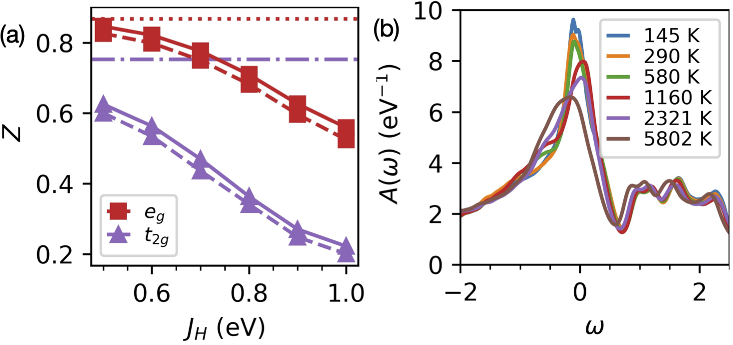
Figure 4: (a) Quasiparticle weight $Z$ of the $t_{2g}$ and $e_{g}$ orbitals are shown as functions of Hund’s coupling $J_{H}$ for LTFS₀ with $U=3.0$ (solid line) and $3.5$ eV (dashed line). The system gradually evolves to a more strongly correlated state with increasing $J_{H}$, while it seems weakly correlated at $J_{H}=0$ with $Z_{t_{2g}}(Z_{e_{g}})=0.75(0.8$7) (dash-dot and dotted line, respectively) (b) Spectral functions projected onto the Fe-$d$ orbitals calculated for different temperatures.

In metallic systems, dynamic correlation effects can be quantified by means of the quasi-particle renormalization factor $Z\approx\left[{\rm 1-Im}\Sigma(i\omega_{0})/\omega_{0}\right]^{-1}$, where $\Sigma(i\omega_{0})$ is the electronic many-body self-energy calculated from DMFT at the first Matsubara frequency. This factor is close to unity for a weakly correlated system, while a small $Z$ indicates a strongly correlated phase. In our case, LTFS₁ is a Mott insulator, albeit with a quite characteristic many-body behavior. For LTFS₀, the calculated value of $Z$ is 0.26 for the $t_{2g}$ orbitals, demonstrating the presence of rather strong correlations even in the metallic phase of this system. This rather strong renormalization of the quasi-particle states in this system stems from the intra-atomic Hund’s exchange coupling $J_{H}$, making LTFS₀ a realization of what in the literature is sometimes called a “Hund’s metal” de’ Medici et al. (2011); Georges et al. (2013), as demonstrated in Fig. 4(a). In this figure, the quasiparticle weight $Z$ as a function of $J_{H}$ is shown for two different interaction strengths, $U=3.0$ and $3.5$ eV. We observe that $Z$ diminishes gradually as $J_{H}$ or $U$ increase with a more pronounced dependency on $J_{H}$. The fact that neither GGA nor GGA$+U$ can capture the electronic ground state or quasi-particle electronic structure and the strong quasiparticle renormalization evidenced by the small $Z$ factor in the metallic LTFS₀ phase allows us to attribute the system to the class of strongly correlated materials. To investigate the nature of the correlations in LTFS₀, we study in more detail the spectra projected onto the Fe-$d$ orbitals, up to high temperature (for fixed lattice constant and atomic positions) Deng et al. (2019). The spectra shown in Fig. 4(b) are characterized by two distinct peaks, namely $t_{2g}$ states near the Fermi level and $e_{g}$ states around an energy of 1.5 eV. As temperature increases, the $t_{2g}$ bands gradually broaden, while their overall shape remains unchanged. This is a distinctive feature from the traditional correlated metal which is near the Mott transition, where two broad side peaks, the so-called Hubbard bands, with gap features develop at high temperatures Deng et al. (2019).

III.3 Average intercalation voltage

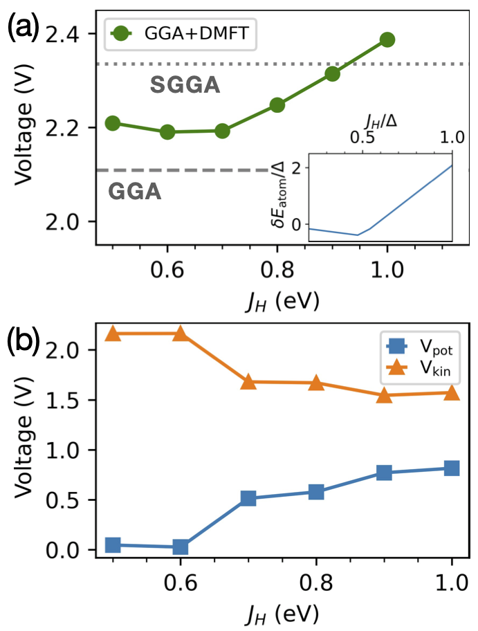
Figure 5: (a) Calculated intercalation voltage as a function of $J_{H}$ obtained from GGA+DMFT (green). The dashed and dotted horizontal lines indicate the calculated voltage via GGA and spin-polarized GGA. (inset) Estimated voltage in atomic limit. See main text for more details. (b) Voltage decomposed into Coulomb interaction energy and kinetic energy contribution.

We now turn to another key quantity of a redox couple of battery materials, the intercalation voltage, which for our systems has been determined experimentally to be around 2.5 eV Saha et al. (2019). In theoretical calculations, the average battery voltage can be evaluated as $V=\left(E({\rm LTFS_{0}})+E({\rm Li})-E({\rm LTFS_{1}})\right)/e$, where the three terms are the total energies of the delithiated system, elemental Li and the lithiated system. We have calculated this quantity using different total energy functionals. The conventional GGA results, 2.11 V, underestimate the experimental value by around $0.37$ eV Saha et al. (2019), while the SGGA result $V=2.34$ V is in better agreement with experiment. An accurate description of the spin state of the Fe-$d$ shell is important not only for the electronic excitations, but also for the energetics, as seen from the difference between GGA and SGGA. The relatively small error of SGGA (without $U$) for this layered sulfide indicates that the strong local Coulomb interactions among the Fe-$d$ electrons are largely screened by the S-$p$ orbitals, having covalent character.

Let us now discuss the impact of the local correlations that govern the behavior of the Fe-$d$ orbitals. Within GGA+DMFT, the calculated voltage is 2.31 V, which is close to the conventional SGGA result. It exhibits only a weak dependence on the Hubbard $U$; for example, $V=$ 2.34 V within GGA+DMFT calculations with $U=3.5$, confirming that the on-site Coulomb interactions are largely screened due to the large Fe-$d$ and S-$p$ orbital hybridisations. However, we will see that the spin state of the valence orbitals, which is determined by $J_{H}$ and the ligand field splitting, are important to describe the properties of the cathode material.

We now turn to the effect of Hund’s coupling $J_{H}$ and the spin-states on the energetics e.g., the operating voltage of the battery. As can be seen from Fig. 5(a), the voltage curve as a function of Hund’s $J_{H}$, while keeping $U=3.0$ eV fixed, shows a V-shape behavior. For small values of the Hund’s exchange $J_{H}$, where LTFS₁ is in the LS state, the voltage decreases at a rate of 0.01 V per 0.1 eV change in $J_{H}$, while in the regime of large $J_{H}$ where LTFS₁ is in the HS phase, the voltage starts to increase by 0.07 V per 0.1 eV $J_{H}$. This behavior can be explained in a simple manner by considering the atomic limit. Assuming an isolated Fe-$d$ shell with nominal electron configuration, one easily obtains (see Appendix B) the V-shape voltage curve as a function of $J_{H}$:

$$\delta E_{\rm atom} =E(d^{6})-E(d^{5})$$

$$\propto\begin{cases}4.89J_{H}-2\Delta,&\text{for }J_{H}/\Delta>0.35\\ -0.82J_{H},&\text{for }J_{H}/\Delta<0.35.\end{cases}$$ (3)

As shown in the inset of Fig. 5(a), the overall trends, including the V-shape behavior and the larger (smaller) slope in the HS (LS) region, are well described in this simple atomic model. Further details can be found in Appendix B. Qualitative differences are observed in the voltage for the LS and HS cases. Fig. 5(b) shows the operating voltage decomposed into the Coulomb interaction $V_{\rm pot}$, where the Hartree and exchange-correlation energies corrected by $+U$ terms are taken into account, and the kinetic energy $V_{\rm kin}$ contribution. For $J_{H}>0.7$ it is clearly seen that the increase in voltage is attributed to the $V_{\rm pot}$ part. In other words, a proper theoretical description of the energy gain from Hund’s interactions in the HS state is a decisive element to capture the operating voltage.

The predictive power of the DFT+DMFT approach is, obviously, limited by the underlying approximations, namely the neglect of non-local correlations – blamed for an underestimation of the voltage within DFT+DMFT in the literature Isaacs and Marianetti (2020) – and ambiguities concerning the double counting corrections and the quality of the charge density used for generating the non-interacting part of the Hamiltonian. For example, GGA+DMFT calculations performed using a Hamiltonian generated with the GGA charge density (or Kohn-Sham Hamiltonian) without charge self-consistency predict a voltage of 1.49 V, greatly underestimating the experimental value. In a previous study, it was noted that non-charge-self-consistent DFT+DMFT calculations could worsen the predicted voltage compared to conventional DFT Isaacs and Marianetti (2020). Nevertheless, our results suggest that the overall energetics needed for a reasonable description of the voltage is captured in our efficient charge-self-consistent DFT+DMFT scheme. In future work, we plan to further investigate the relative effects of non-local correlation vs charge-redistribution using more sophisticated methods such as $GW$+DMFT, which allow for progress both concerning a better description of the quasi-particle band structures and the double counting issue.

IV Conclusion

We have performed DFT+DMFT calculations using an efficient charge-self-consistent scheme to investigate the electronic structure, local properties, and intercalation voltage of the Li-rich layered sulfides Li_x[Li_0.33-2y/3Ti_0.67-y/3Fe_y]S₂. A careful comparison between results using different methods, including spin-averaged and spin-polarized GGA, and GGA+DMFT was made. Both of the end members, namely the fully discharged Li_1.11Ti_0.56Fe_0.33S₂ and the fully charged compound Li_0.11Ti_0.56Fe_0.33S₂, are strongly correlated systems, identified as high-spin Mott-insulator and low-spin correlated metal, respectively. We have shown that dynamical correlations originating from Hund’s exchange coupling $J_{H}$ are important to describe this class of materials, while the effective local Hubbard $U$ is largely screened. The impact of $J_{H}$ on the intercalation voltage may suggest new pathes for designing higher-energy lithium ion-battery cathode materials. To our knowledge, this is the first demonstration of Hund’s physics playing a crucial role in the electrochemcial properties of real-life battery materials. A deeper understanding of these effects will hopefully contribute to paving the way to better battery materials in the future.

Appendix A Computational details

By using DFT within the VASP Kresse and Furthmüller (1996) code and DFT+DMFT implemented in the DMFTpack software combined with OpenMX _DM ; ope ; Sim and Han (2019) and the impurity solver implemented in Ref. Haule, 2007, we have studied the electronic and magnetic properties of Li_x[Li_0.33-2y/3Ti_0.67-y/3Fe_y]S₂. The DFT calculations were performed within the generalized gradient approximation as parameterized by Perdew, Burke and Ernzerhof (GGA-PBE) Perdew et al. (1996). The D3 method of Grimme et al. was used for van der Waals corrections Grimme et al. (2010, 2011) Atomic positions were relaxed with a force criterion of 1 meV/Å. The lattice constants are fixed to the experimental values: $a=b=3.54$ Å and $a=b=3.35$ Å for the discharged ($x=1$) and fully charged ($x=0$) phases, respectively Saha et al. (2019). $13\times 13\times 8$ k-points were used in the Brillouin zone for the momentum space integrations.

To describe electronic correlation effects, the GGA$+U$ Anisimov et al. (1991, 1993) and single-site paramagnetic GGA+DMFT Anisimov et al. (1997); Lichtenstein and Katsnelson (1998) have been employed. The interaction part of the Hamiltonian for the d-shell reads:

$$H_{{\rm int}}= \frac{1}{2}\sum_{\sigma,m,m^{\prime}}U_{mm^{\prime}}n_{m\sigma}n_{m^{\prime}\bar{\sigma}}$$

$$+\frac{1}{2}\sum_{\sigma,m\neq m^{\prime}}(U_{mm^{\prime}}-J_{mm^{\prime}})n_{m\sigma}n_{m^{\prime}\sigma}.$$ (4)

Here the direct and exchange interaction parameters, $U_{mm^{\prime}}$ and $J_{mm^{\prime}}$, are parameterized by the Slater integrals of the $d$-shell, namely $F_{0},$ $F_{2}$, and $F_{4}$ Pavarini (2011). We present our results in terms of the $U=F_{0}$ and $J_{H}=(F_{2}+F_{4})/14$, within the assumption $F_{4}/F_{2}=0.625$. Unless otherwise stated, calculations were performed with $U=3.0$, $J_{H}=0.9$, and FLLnS double counting : $\Sigma_{DC}^{\rm FLLnS}=U(N-\frac{1}{2})-J(\frac{N}{2}-\frac{1}{2})$ Ylvisaker et al. (2009); Ryee and Han (2018). The charge-density-only GGA$+U$ should be distinguished from other DFT$+U$ flavors such as spin-polarized GGA$+U$ Liechtenstein et al. (1995) and the Dudarev’s simplified DFT$+U$ method Dudarev et al. (1998); Han et al. (2006). The interaction parameters, $U$ and $J_{H}$, used in this work are consistent with that used in the previous study, $U_{\text{eff}}=U-J_{H}=2.0$ eV Saha et al. (2019) and in reasonable range compared to other iron-based compounds van Roekeghem et al. (2016). The ferromagnetic ground state, with a lower energy of 3 meV than the antiferromagnetic state at $U=3.0$ and $J_{H}=0.9$ eV, is assumed for various $U$ and $J_{H}$ parameters.

In our single site DMFT calculation, a natural atomic orbitals projector onto to Fe-$d$ orbitals with an energy window of $W=[-6,5]$ eV containing Fe-$d$ and S-$p$ orbitals has been employed Sim and Han (2019). The self-energy is decomposed into three $10\times 10$ matrices corresponding to three inequivalent Fe atoms in the unit cell, i.e., $\Sigma(i\omega_{n})=\oplus_{i=1}^{3}\Sigma_{{\rm Fe(i)}}(i\omega_{n})$. $\Sigma_{{\rm Fe(i)}}(i\omega_{n})$ is determined from the fictitious impurity problem with self-consistency condition. The impurity problems are solved by employing a hybridization expansion continuous-time quantum Monte Carlo (CT-QMC) Werner et al. (2006); Werner and Millis (2006) algorithm implemented in Ref. Haule (2007). The self-energy in the real frequency domain is obtained from the Matsubara self-energy by analytic continuation using the maximum quantum entropy method Sim and Han (2018), extending the maximum entropy method to matrix valued Green’s functions Jarrell and Gubernatis (1996); Gunnarsson et al. (2010).

Appendix B On-site Coulomb energy in DFT+$U$ and DFT+DMFT

In this section we calculate the total energy contribution from the on-site interaction $\Delta E_{U}=\braket{H_{{\rm int}}}-E_{{\rm DC}}$. For simplicity, in this section the interaction $H_{{\rm int}}$ is assumed to be of Slater-Kanamori form with $U_{SK}=U+8J_{H}/7,$ $J_{SK}=5J_{H}/7$, and $U^{\prime}_{SK}=U_{SK}-2J_{SK}$ Pavarini (2011); Isaacs and Marianetti (2020).

DFT$+U$

$E_{{\rm int}}^{U}=\frac{U}{2}\sum_{(\alpha\sigma)\neq(\beta\sigma\prime)}n_{\alpha\sigma}n_{\beta\sigma^{\prime}}-\frac{J_{H}}{2}\sum_{\sigma}\sum_{\alpha\neq\beta}n_{\alpha\sigma}n_{\beta\sigma}$ and the double counting term is $E^{{\rm DC}}_{{\rm FLLnS}}=\frac{U}{2}N(N-1)-\frac{J}{2}\sum_{\sigma}\frac{N}{2}(\frac{N}{2}-1)$, where $n_{\alpha\sigma}$ is an eigenvalue of the occupation number matrix with orbital index $\alpha$ and spin $\sigma$. $N=\sum_{\sigma}N^{\sigma}=\sum_{\sigma}\sum_{\alpha}n_{\alpha\sigma}$. The Coulomb energy correction $\Delta E^{U}=E_{int}^{U}-E_{{\rm DC}}$ can be written as follows:

$$\Delta E^{U}=\frac{1}{2}(U-J)\sum_{\alpha\sigma}(n_{\alpha\sigma}-n_{\alpha\sigma}^{2})-\frac{J}{4}M^{2},$$

where $M=N_{\uparrow}-N_{\downarrow}$ is the magnetic moment of the localized $d$-orbitals. We note that the first term is obtained from the double counting energy $E_{{\rm DC}}^{{\rm FLL}}$ Han et al. (2006). The second term imposes an energy gain due to the finite magnetic moment $M$, leading to a magnetic polarization, which is not included in the non-spin polarized GGA exchange-correlation functional.

In DMFT, the Coulomb interaction energy is beyond the HF approximation. $E_{{\rm int}}^{{\rm DMFT}}=\frac{U}{2}\braket{\hat{N}^{2}-\hat{N}}-\frac{J_{H}}{2}\sum_{\sigma}\braket{\hat{N_{\sigma}}^{2}-\hat{N_{\sigma}}}$. After some algebra, using $E_{\text{DC}}^{\text{FLLnS}}$, we obtain

$$\Delta E^{{\rm DMFT}}=\frac{1}{2}(U-J)\sum_{\alpha\sigma}(\braket{\delta N^{2}})-\frac{J}{4}M_{{\rm eff}}^{2},$$

where $\braket{\delta N^{2}}=\braket{N^{2}}-\braket{N}^{2}$ and $M_{{\rm eff}}=(N^{2}-4\braket{N_{\uparrow}N_{\downarrow}})^{1/2}$. We can see that within the HF approximation, $\braket{N_{\uparrow}N_{\downarrow}}\approx N_{\uparrow}N_{\downarrow}$, $M_{{\rm eff}}$ is equivalent to the conventional magnetization, namely $M_{{\rm eff}}=N_{\uparrow}-N_{\downarrow}$.

Atomic limit

Three different configurations, namely, $d^{6}$(HS), $d^{6}$(LS), and $d^{5}$(LS) are concerned. Here, the $d^{6}$(HS) and $d^{5}$(LS) configurations are expected as ground state configurations of Fe in LTFS₁ and LTFS₀, respectively. Assuming FLL-nS double counting, one can see that $\Delta E_{U}$ can be expressed as:

$$\Delta E_{U}\approx\begin{cases}-4J_{H}+2\bar{\Delta}&d^{6}(HS)\\ 1.71J_{H}&d^{6}(LS)\\ 0.89J_{H}&d^{5}(LS)\end{cases}.$$ (5)

Given these expressions, we can estimate $J_{H}$ dependence of the Coulomb energy contribution to the voltage for different atomic configurations. Interestingly, our DFT+DMFT results show similar trends for the transition from the $d^{6}$ to the $d^{5}$(LS) configuration:

$$V_{LS}=E(d^{6})-E(d^{5})\propto \begin{cases}4.89J_{H},&\text{for }J_{H}/\Delta>0.35\\ -0.82J_{H},&\text{otherwise}.\end{cases}$$ (6)

References

- Mizushima et al. (1980) K Mizushima, P C Jones, P J Wiseman, and J B Goodenough, “LixCoO2 : A new cathode material for batteries of high energy density,” Mater. Res. Bull. 15, 783 (1980).
- Lu et al. (2001) Zhonghua Lu, D. D. MacNeil, and J. R. Dahn, “Layered Cathode Materials Li[NixLi(1/3-2x/3)Mn(2/3-x/3)]O2 for Lithium-Ion Batteries,” Electrochem. Solid-State Lett. 4, A191 (2001).
- Assat and Tarascon (2018) Gaurav Assat and Jean-Marie Tarascon, “Fundamental understanding and practical challenges of anionic redox activity in Li-ion batteries,” Nat Energy 3, 373–386 (2018).
- Li and Xia (2017) Biao Li and Dingguo Xia, “Anionic Redox in Rechargeable Lithium Batteries,” Adv. Mater. 29, 1701054 (2017).
- Thackeray et al. (2007) Michael M. Thackeray, Sun-Ho Kang, Christopher S. Johnson, John T. Vaughey, Roy Benedek, and S. A. Hackney, “Li2MnO3-stabilized LiMO2 (M = Mn, Ni, Co) electrodes for lithium-ion batteries,” J. Mater. Chem. 17, 3112 (2007).
- Saha et al. (2019) Sujoy Saha, Gaurav Assat, Moulay Tahar Sougrati, Dominique Foix, Haifeng Li, Jean Vergnet, Soma Turi, Yang Ha, Wanli Yang, Jordi Cabana, Gwenaëlle Rousse, Artem M. Abakumov, and Jean-Marie Tarascon, “Exploring the bottlenecks of anionic redox in Li-rich layered sulfides,” Nat Energy 4, 977 (2019).
- Metzner and Vollhardt (1989) Walter Metzner and Dieter Vollhardt, “Correlated Lattice Fermions in Dimensions,” Phys. Rev. Lett. 62, 324 (1989).
- Georges and Kotliar (1992) Antoine Georges and Gabriel Kotliar, “Hubbard model in infinite dimensions,” Phys. Rev. B 45, 6479 (1992).
- Zhang et al. (1993) X. Y. Zhang, M. J. Rozenberg, and G. Kotliar, “Mott transition in the Hubbard model at zero temperature,” Phys. Rev. Lett. 70, 1666 (1993).
- Anisimov et al. (1997) V. I. Anisimov, A. I. Poteryaev, M. A. Korotin, A. O. Anokhin, and G. Kotliar, “First-principles Calculations of the Electronic Structure and Spectra of Strongly Correlated Systems: Dynamical Mean-field Theory,” J Phys Condens Matter 9, 7359 (1997).
- Lichtenstein and Katsnelson (1998) A. I. Lichtenstein and M. I. Katsnelson, “Ab initio calculations of quasiparticle band structure in correlated systems: LDA++ approach,” Phys. Rev. B 57, 6884 (1998).
- Anisimov et al. (1991) Vladimir I. Anisimov, Jan Zaanen, and Ole K. Andersen, “Band theory and Mott insulators: Hubbard instead of Stoner ,” Phys. Rev. B 44, 943 (1991).
- Liechtenstein et al. (1995) A. I. Liechtenstein, V. I. Anisimov, and J. Zaanen, “Density-functional theory and strong interactions: Orbital ordering in Mott-Hubbard insulators,” Phys. Rev. B 52, R5467–R5470 (1995).
- de’ Medici et al. (2011) Luca de’ Medici, Jernej Mravlje, and Antoine Georges, “Janus-Faced Influence of Hund’s Rule Coupling in Strongly Correlated Materials,” Phys. Rev. Lett. 107, 256401 (2011).
- Georges et al. (2013) Antoine Georges, Luca de’Medici, and Jernej Mravlje, “Strong Correlations from Hund’s Coupling,” Annu. Rev. Condens. Matter Phys. 4, 137–178 (2013).
- Georges et al. (1996) Antoine Georges, Gabriel Kotliar, Werner Krauth, and Marcelo J. Rozenberg, “Dynamical mean-field theory of strongly correlated fermion systems and the limit of infinite dimensions,” Rev. Mod. Phys. 68, 13–125 (1996).
- Anisimov et al. (1993) V. I. Anisimov, I. V. Solovyev, M. A. Korotin, M. T. Czyżyk, and G. A. Sawatzky, “Density-functional theory and NiO photoemission spectra,” Phys. Rev. B 48, 16929 (1993).
- Ylvisaker et al. (2009) Erik R. Ylvisaker, Warren E. Pickett, and Klaus Koepernik, “Anisotropy and magnetism in the LSDA + U method,” Phys. Rev. B 79, 035103 (2009).
- Werner et al. (2006) Philipp Werner, Armin Comanac, Luca de’ Medici, Matthias Troyer, and Andrew J. Millis, “Continuous-Time Solver for Quantum Impurity Models,” Phys. Rev. Lett. 97, 076405 (2006).
- Werner and Millis (2006) Philipp Werner and Andrew J. Millis, “Hybridization expansion impurity solver: General formulation and application to Kondo lattice and two-orbital models,” Phys. Rev. B 74, 155107 (2006).
- Ryee and Han (2018) Siheon Ryee and Myung Joon Han, “The effect of double counting, spin density, and Hund interaction in the different DFT+U functionals,” Sci. Rep. 8, 9559 (2018).
- Dudarev et al. (1998) S. L. Dudarev, G. A. Botton, S. Y. Savrasov, C. J. Humphreys, and A. P. Sutton, “Electron-energy-loss spectra and the structural stability of nickel oxide: An LSDA+U study,” Phys. Rev. B 57, 1505–1509 (1998).
- Pavarini (2011) Eva Pavarini, ed., The LDA+DMFT Approach to Strongly Correlated Materials: Autumn School Organized by the DFG Research Unit 1346 Dynamical Mean-Field Approach with Predictive Power for Strongly Correlated Materials at Forschungszentrum Jülich, 4-7 October 2011 ; Lecture Notes, Schriften Des Forschungszentrums Jülich Reihe Modeling and Simulation No. 1 (Forschungszentrum Jülich, Jülich, 2011).
- Chen et al. (2015) Jia Chen, Andrew J. Millis, and Chris A. Marianetti, “Density functional plus dynamical mean-field theory of the spin-crossover molecule Fe(phen) 2 (NCS) 2,” Phys. Rev. B 91, 241111 (2015).
- Park et al. (2014) Hyowon Park, Andrew J. Millis, and Chris A. Marianetti, “Total energy calculations using DFT+DMFT: Computing the pressure phase diagram of the rare earth nickelates,” Phys. Rev. B 89 (2014).
- Chen and Millis (2016) Hanghui Chen and Andrew J. Millis, “Spin-density functional theories and their + U and + J extensions: A comparative study of transition metals and transition metal oxides,” Phys. Rev. B 93, 045133 (2016).
- Momma and Izumi (2011) Koichi Momma and Fujio Izumi, “VESTA3 for three-dimensional visualization of crystal, volumetric and morphology data,” J. Appl. Crystallogr. 44, 1272–1276 (2011).
- Watanabe et al. (2019) Eriko Watanabe, Wenwen Zhao, Akira Sugahara, Benoit Mortemard de Boisse, Laura Lander, Daisuke Asakura, Yohei Okamoto, Takashi Mizokawa, Masashi Okubo, and Atsuo Yamada, “Redox-Driven Spin Transition in a Layered Battery Cathode Material,” Chem. Mater. 31, 2358–2365 (2019).
- Seo et al. (2016) Dong-Hwa Seo, Jinhyuk Lee, Alexander Urban, Rahul Malik, ShinYoung Kang, and Gerbrand Ceder, “The structural and chemical origin of the oxygen redox activity in layered and cation-disordered Li-excess cathode materials,” Nature Chem 8, 692–697 (2016).
- Deng et al. (2019) Xiaoyu Deng, Katharina M. Stadler, Kristjan Haule, Andreas Weichselbaum, Jan von Delft, and Gabriel Kotliar, “Signatures of Mottness and Hundness in archetypal correlated metals,” Nature Communications 10, 2721 (2019).
- Isaacs and Marianetti (2020) Eric B. Isaacs and Chris A. Marianetti, “Compositional phase stability of correlated electron materials within DFT + DMFT,” Phys. Rev. B 102, 045146 (2020).
- Kresse and Furthmüller (1996) G. Kresse and J. Furthmüller, “Efficient iterative schemes for ab initio total-energy calculations using a plane-wave basis set,” Phys. Rev. B 54, 11169–11186 (1996).
- (33) “DMFTpack,” https://kaist-elst.github.io/DMFTpack/.
- (34) “OpenMX,” http://www.openmx-square.org.
- Sim and Han (2019) Jae-Hoon Sim and Myung Joon Han, “Density functional theory plus dynamical mean-field theory with natural atomic orbital projectors,” Phys. Rev. B 100, 115151 (2019).
- Haule (2007) Kristjan Haule, “Quantum Monte Carlo impurity solver for cluster dynamical mean-field theory and electronic structure calculations with adjustable cluster base,” Phys. Rev. B 75, 155113 (2007).
- Perdew et al. (1996) John P. Perdew, Kieron Burke, and Matthias Ernzerhof, “Generalized Gradient Approximation Made Simple,” Phys. Rev. Lett. 77, 3865 (1996).
- Grimme et al. (2010) Stefan Grimme, Jens Antony, Stephan Ehrlich, and Helge Krieg, “A consistent and accurate ab initio parametrization of density functional dispersion correction (DFT-D) for the 94 elements H-Pu,” The Journal of Chemical Physics 132, 154104 (2010).
- Grimme et al. (2011) Stefan Grimme, Stephan Ehrlich, and Lars Goerigk, “Effect of the damping function in dispersion corrected density functional theory,” J. Comput. Chem. 32, 1456–1465 (2011).
- Han et al. (2006) Myung Joon Han, Taisuke Ozaki, and Jaejun Yu, “O() LDA+ electronic structure calculation method based on the nonorthogonal pseudoatomic orbital basis,” Phys. Rev. B 73, 045110 (2006).
- van Roekeghem et al. (2016) Ambroise van Roekeghem, Loïg Vaugier, Hong Jiang, and Silke Biermann, “Hubbard interactions in iron-based pnictides and chalcogenides: Slater parametrization, screening channels, and frequency dependence,” Phys. Rev. B 94, 125147 (2016).
- Sim and Han (2018) Jae-Hoon Sim and Myung Joon Han, “Maximum quantum entropy method,” Phys. Rev. B 98, 205102 (2018).
- Jarrell and Gubernatis (1996) M. Jarrell and J. E. Gubernatis, “Bayesian inference and the analytic continuation of imaginary-time quantum Monte Carlo data,” Phys. Rep. 269, 133 (1996).
- Gunnarsson et al. (2010) O. Gunnarsson, M. W. Haverkort, and G. Sangiovanni, “Analytical continuation of imaginary axis data using maximum entropy,” Phys. Rev. B 81, 155107 (2010).