Generative Adversarial Networks for Spatio-Spectral Compression of Hyperspectral Images

Abstract

The development of deep learning-based models for the compression of hyperspectral images (HSIs) has recently attracted great attention in remote sensing due to the sharp growing of hyperspectral data archives. Most of the existing models achieve either spectral or spatial compression, and do not jointly consider the spatio-spectral redundancies present in HSIs. To address this problem, in this paper we focus our attention on the High Fidelity Compression (HiFiC) model (which is proven to be highly effective for spatial compression problems) and adapt it to perform spatio-spectral compression of HSIs. In detail, we introduce two new models: i) HiFiC using Squeeze and Excitation (SE) blocks (denoted as HiFiC_SE); and ii) HiFiC with 3D convolutions (denoted as HiFiC_3D) in the framework of compression of HSIs. We analyze the effectiveness of HiFiC_SE and HiFiC_3D in compressing the spatio-spectral redundancies with channel attention and inter-dependency analysis. Experimental results show the efficacy of the proposed models in performing spatio-spectral compression, while reconstructing images at reduced bitrates with higher reconstruction quality. The code of the proposed models is publicly available at https://git.tu-berlin.de/rsim/HSI-SSC.

Index Terms—  Spatio-spectral image compression, high fidelity compression, deep learning, hyperspectral images.

1 Introduction

As a result of rapid evolution of hyperspectral imaging technologies, the volume of hyperspectral data archives significantly increases. Hyperspectral sensors can acquire images characterized by a very high spectral resolution that results in hundreds of observation channels. Dense spectral information provided in hyperspectral images (HSIs) leads to a very high capability for the identification and discrimination of the materials in a given scene. This makes the use of hyperspectral images very important in a wide variety of remote sensing (RS) applications. However, the huge amount of data results in a heavy burden for the storage and transmission of HSIs [1]. Accordingly, the development of efficient compression techniques that encode the data into fewer bits with minimal loss of information is a growing research interest in RS.

There are several hyperspectral image compression methods, which can be grouped into two categories: i) traditional approaches; and ii) learning-based approaches. Traditional approaches mostly rely on transform coding. As an example, in [2] HSIs are compressed by applying the JPEG 2000 [3] algorithm in combination with a principal component analysis that is applied for spectral decorrelation as well as spectral dimensionality reduction. Lim et. al [4] apply a three dimensional wavelet transform to compress the HSIs. Abousleman et al. [5] use differential pulse code modulation to spectrally decorrelate the data while a 2D discrete cosine transform coding scheme is used for spatial decorrelation. The current state of the art in learning-based hyperspectral image compression is formed by convolutional autoencoders (CAEs) [6, 7, 8, 9] that reduce the dimensionality of the latent space by sequentially applying convolutions (convs) and downsampling operations. There are several CAE-based models developed in RS. As an example, in [6, 7], a 1D-CAE model that only compresses the spectral content by stacking multiple 1D convs combined with two pooling layers and LeakyReLU activation functions is introduced. In [8] a novel spectral signal compressor network (SSCNet), which incorporates spatial compression by utilizing 2D convs, PReLUs and 2D max poolings for encoding and strided 2D transposed convs for decoding, is presented. In [9], a 3D-CAE that combines spatial and spectral compression is introduced. That network is built by strided 3D convs, LeakyReLU, 3D batch normalization, residual blocks and upsampling layers in the decoder. However, due to the fixed compression ratio of CAEs and their relatively high bitrates, there is a need for developing more effective approaches.

(a) HiFiC architecture [10]

(b) Encoder (E)

(c) Generator (G)

(d) Discriminator (D)

Fig. 1: 1(a) The overall GAN-based HiFiC model architecture [10]. 1(b), 1(c) and 1(d) The Encoder (E), Generator (G) and Discriminator (D) architectures of HiFiC_opt, HiFiC_SE with added SE Blocks and HiFiC_3D with two Conv3D layers, respectively. Q: quantization, P: probability model, AE: arithmetic encoder, AD: arithmetic decoder, Conv3D(T)-N-KxK(xK): 2D/3D (transposed) convolution layer with N output channels and kernel size K, $\downarrow^{2}$/$\uparrow_{2}$: stride 2, CNorm: channel normalization layer, NN-$\uparrow_{16}$: nearest neighbor upsampling.

To address the limitations of CAEs associated to high bitrates, generative adversarial network (GAN)-based image compression models [10, 11] have been found successful in the computer vision (CV) community. GANs are capable of producing visually convincing results that are perceptually similar to the input image, and thus GAN-based compression shows improved performance in spatial compression even at extremely low bitrates keeping intact the perceptual quality of the reconstructed image. However, the applicability of GANs in spatio-spectral compression of HSIs has not been studied yet.

In this paper, we focus our attention on GANs and investigate their effectiveness for spatio-spectral compression of HSIs. We select the state-of-the-art high performance GAN-based High Fidelity Compression (HiFiC) [10] as our base model. HiFiC consists of blocks with 2D convs and thus treats each band separately to perform band-by-band spatial compression. To effectively compress the spectral and spatial information content of HSIs, we introduce two new models: i) HiFiC_SE using queeze and Excitation (SE) blocks [12]; and ii) HiFiC_3D using 3D convs that can exploit both spatial and spectral redundancies. The SE blocks reduce feature redundancies using channel attention while 3D convs use 3D kernels to learn feature dependencies across the channels. Thus, the proposed models are capable of accurately learning to compress spatial and spectral redundancies in HSIs. Experimental results show that proposed models achieve low bitrates with good perceptual reconstruction capability.

2 Proposed Models for Spatio-Spectral HSI Compression

Let $\textbf{X}=\{x_{i}\}_{i=1}^{H}$ be a set of $H$ uncompressed HSIs, where $x_{i}$ is the $i^{th}$ image. The aim of spatio-spectral compression is to produce spatially and spectrally decorrelated latent representations $\textbf{Y}=\{y_{i}\}_{i=1}^{H}$ that can be entropy coded and stored with minimal number of bits. At the same time, the learned representations should retain all the necessary information for reconstructing back $\textbf{X}^{\prime}=\{x_{i}^{\prime}\}_{i=1}^{H}$ with the least possible distortion.

In this paper, we introduce HiFiC_SE and HiFiC_3D for the spatio-spectral hyperspectral image compression. Both models are defined in the framework of a HiFiC model [10]. The base HiFiC model includes 4 modules: i) encoder $E$; ii) probability model $P$; iii) generator $G$; and iv) discriminator $D$ (see Figure 1). The proposed HiFiC_SE and HiFiC_3D models follow the base HiFiC but include modifications on the architectures of $E$ and $G$ using SE blocks and 3D convs, respectively (see 1(b) and 1(c)). We introduce these modifications to the architectures to specifically exploit spatio-spectral redundancies. The HiFiC_SE consists of SE blocks prior to the regular 2D convs that enable it to attend to the spectral channel information. The SE block consists of layers of global pooling, Fully Connected Multi-Layer Perceptron (FC-MLP) with ReLU activation, where neuron numbers are decreased by reduction ratio $r_{r}$, followed by another FC-MLP with Sigmoid activation which outputs weights for each channel (see Figure 2). The SE block investigates the relationship between channels by explicitly modelling the inter-dependencies between them. We use $l_{1}$ regularization at the FC-MLP layers for generating sparse weights indicating the channel importance. These weights are then applied to the feature maps to generate the output of the SE block, which can be fed directly into subsequent layers of the network. The HiFiC_3D is built by replacing the first 2D convs of the Encoder (E) and the last 2D conv of the Generator (G) with 3D convs where the 3D kernels can evaluate spectral redundancies (see 1(b) and 1(c)). It is inspired from the video compression work in [13] that uses 3D convs to remove temporal redundancies.

Fig. 2: The basic structure of an SE block [12].

Given an image $x_{i}\in\textbf{X}$, it is encoded to a spatially and spectrally decorrelated latent representation $y_{i}$ and then decoded back to $x_{i}^{\prime}$ as:

$$y_{i}=Q(E(x_{i})),\;x_{i}^{\prime}=G(y_{i})$$ (1)

$Q$ is a quantizer that is modeled as rounding operation during inference and straight-through estimator [14] during training. In the bottleneck of the network, the latents $y_{i}$ are entropy coded into bitstreams using arithmetic encoding (AE) with minimum bitrate $r(y_{i})=-\log(P(y_{i}))$ where $P$ follows the hyper-prior model in [15] with side information. The bitstreams are further decoded back to $y_{i}$ using arithmetic decoding (AD). Finally, a single-scale discriminator $D$ with the conditional information ($y_{i}$) decides if the reconstructed image is real or generated. Each of the modules $E$, $P$, $G$, and $D$ is parameterized by convolutional neural networks and optimized together to obtain the minimum rate-distortion (RD) trade-off. The loss functions $L$ for optimization of each of the four blocks are as follows:

$$L_{\scriptscriptstyle E,G,P}=\mathbb{E}_{\scriptscriptstyle x_{i}\sim P_{\bf{X}}}[\lambda r(y_{i})+d(x_{i},x_{i}^{\prime})-\beta\log D(x_{i}^{\prime},y_{i})]$$ (2)

$$L_{\scriptscriptstyle D}=\mathbb{E}_{\scriptscriptstyle x_{i}\sim P_{\bf{X}}}[-\log(1-D(x_{i}^{\prime},y_{i}))]+\mathbb{E}_{\scriptscriptstyle x_{i}\sim P_{\bf{X}}}[-\log D(x_{i},y_{i})]\\$$ (3)

where $r(y_{i})$ is the rate, $d(x_{i},x_{i}^{\prime})$ is the distortion loss, $\lambda$ is the hyperparameter controlling the RD trade-off, and $\log(D(x_{i}^{\prime},y_{i}))$ is the conditional discriminator loss with $\beta$ controlling the discriminator loss effect. The distortion loss is modelled as:

$$d(x_{i},x_{i}^{\prime})=\theta_{1}\cdot\textsc{MSE}+\theta_{2}\cdot(1-\textsc{SSIM})+\theta_{3}\cdot\textsc{LPIPS}$$ (4)

where $\theta$’s are hyperparameters that control the effect of mean square error (MSE), structural similarity index (SSIM) [16], and learned perceptual image patch similarity (LPIPS) [17] losses in the total distortion loss calculation. The LPIPS loss mimics the human visual system and measures reconstruction quality in the feature space, while the SSIM loss is added as an improvement to HSI compression as it enhances reconstruction by preserving the structural information relevant in the scene.

Since $r(y_{i})$ is at odds with $d(x_{i},x_{i}^{\prime})$ and $-\log(D(x_{i}^{\prime},y_{i}))$ in (2), controlling the RD trade-off is difficult (as for a fixed $\lambda$, different $\theta$’s and $\beta$ would result in models with different bitrates). Hence, we use target bitrates $r_{t}$ as in [10] and control $\lambda$ using $\lambda^{(a)}$ and $\lambda^{(b)}$ with the following rule:

$$\lambda=\begin{cases}\lambda^{(a)},&\text{if $r(y_{i})>r_{t}$}\\ \lambda^{(b)},&\text{otherwise}\end{cases}$$ (5)

with $\lambda^{(a)}\gg\lambda^{(b)}$ the model learns bitrates closer to $r_{t}$. By keeping $\lambda^{(b)}$ fixed and changing only $r_{t}$ and $\lambda^{(a)}$, it is possible to achieve different bitrates.

3 Dataset Description and Design of Experiments

To evaluate the effectiveness of our proposed models, the experiments have been conducted by using a hyperspectral dataset that consists of 3,840 image patches with 369 spectral bands (which cover the visible and near-infrared portion of the electromagnetic spectrum in the wavelength range between 400 - 1,000 nm). Each patch is a section of 96 x 96 pixels with a spatial resolution of 28cm. We normalized the data between 0 - 1, which is required for our compression models. The patches were then split in the ratio of 80%, 10% and 10% to form train, validation and test set, respectively.

All the experiments were carried out using a NVIDIA Tesla V100 GPU with 32 GBs of memory. The code for the compression model was implemented with TensorFlow v1.15.2 and built on TensorFlow Compression v1.3 [18] and HiFiC [10]. We trained all the models with Adam optimizer with a batch size of 8. We use a baseline model trained without GAN ($\beta=0$ in (2)) as an initializer for each of our models. For the distortion loss in (4) we used $\theta_{1}=0.15\cdot 2^{-5}$, $\theta_{2}=0.075\cdot 2^{-3}$ and $\theta_{3}=1$. These values were determined through multiple experiments. The discriminator loss effect $\beta$ was set to 0.15, while the reduction ratio $r_{r}$ in the SE block was selected as 2. As mentioned in Section 2, different bitrates can be achieved by changing two hyperparameters: i) target rate $r_{t}$; and ii) $\lambda^{(a)}$. The target rates $r_{t}$ was varied from [0.2,1] with a step size of 0.2 with its associated $\lambda^{(a)}$ values set accordingly. In total, we configured five settings for each model with different $r_{t}$ and $\lambda^{(a)}$ combinations (see Table 1).

Table 1: List of target rates $r_{t}$’s and its associated $\lambda^{(a)}$ values.

$r_{t}$	0.2	0.4	0.6	0.8	1
$\lambda^{(a)}$	$2^{1}$	$2^{0}$	$2^{-1}$	$2^{-2}$	$2^{-3}$

Table 2: Performance analysis with placement of SE and 3D conv blocks in the HiFiC_SE and HiFiC_3D models, respectively.

SE block placement	PSNR	Runtime
	(in dB)	(iters/s)
HiFiCSE - $E$: initial layer	29.80	7.84
HiFiCSE - $E$: initial+after Norm	30.12	7.49
HiFiCSE - $E$ and $G$: after Norm	30.89	7.01
HiFiC3D - $E$ and $G$: all places	30.12	7.31
HiFiC3D - $E$: initial and $G$: final	29.24	9.25

(a)	(b)	(c)

Fig. 3: (a) Original image; (b) reconstructed image without 3D convs; and (c) reconstructed image with 3D convs. Bottom row shows the close-ups of the top image parts.

We have compared the proposed spatio-spectral compression models (HiFiC_SE and HiFiC_3D) with: i) the adapted (with the loss in (4)) and optimized spatial compression HiFiC model (termed as HiFiC_opt); and ii) the traditional JPEG 2000. The comparison was performed at different bitrates and the compression quality was analysed using the reconstruction performance measured using peak signal-to-noise ratio (PSNR) and the compression rate achieved in terms of bitrate measured in bits per pixel (bpp). The higher the PSNR and lower the bpp the better the compression performance. We would like to note that we could not report comparison results with CAE models [6, 7, 8, 9], since they operate at much higher bitrates than our proposed model.

4 Experimental Results

4.1 Ablation Study

In this subsection, we present an ablation study to assess the impact of the choice of placement of SE blocks and 3D convs in the base HiFiC model. The performance is evaluated in terms of reconstruction quality measured with average PSNR and runtime measured as average number of iterations completed per second (iters/s: the higher the value the faster the model) to decide the best placement. The obtained metric by placing the SE and 3D blocks at different layers in the model is provided in Table 2. For this, the SE blocks were placed in the initial layer of $E$ alone. Then, we placed it in the initial layer and after every normalization layer in $E$, and finally we extended SE blocks to cover all layers in $E$ and $G$ after every normalization layer. One may observe that the best PSNR performance with comparable runtime to other placements is achieved when the SE block was incorporated in both $E$ and $G$ after the normalization layer.

Fig. 4: Rate-distortion performance of our proposed HiFiC_SE and HiFiC_3D compared to HiFiC_opt and JPEG2000.

	(29.17, 0.82)	(29.34, 1.66)	(30.33, 0.55)
(a)	(b)	(c)	(d)

Fig. 5: (a) Original image. Reconstructed images with (b) HiFiC_opt, (c) HiFiC_SE and (d) HiFiC_3D. The PSNR and achieved bpp are shown below each image as (PSNR in dB, bpp).

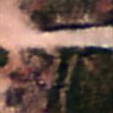
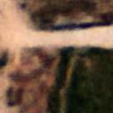
(a)	(27.40, 0.25) (29.80, 0.56) (29.90, 1.74) (33.02, 1.78) (31.54, 1.63) (28.85, 0.26) (29.87, 0.53) (33.60, 0.78) (32.24, 1.22) (31.92, 1.43) (b) (c) (d) (e) (f)

Fig. 6: (a) Original image. Reconstructed results with HiFiC_SE (first row) and HiFiC_3D (second row) at $r_{t}$: (b) 0.2 (c) 0.4 (d) 0.6 (e) 0.8 and (f) 0.1. The PSNR and achieved bpp are shown below each image as (PSNR in dB, bpp).

4.2 Spatio-Spectral HSI Compression

In this subsection, we evaluate the efficacy of our proposed spatio-spectral hyperspectral image compression models. As a first step we analyse the importance of replacing 3D conv layers in the GANs for reconstruction. Fig 3 shows the reconstructed images with HiFiC_SE and HiFiC_3D using the GAN. The reconstruction without 3D conv layers in Figure 3(b) fails to generate the spatial information characterized by the texture and geometrical characteristics of the objects within images. But with the integrated 3D conv layers in Figure 3(c) the perceptual quality is improved and the texture content is better represented. In addition, high quality compressed images are obtained with reduced perceptible artifacts. This shows the importance of the 3D convs in GAN-based models for HSI compression. Figure 4 shows the rate-distortion curves for the spatio-spectral compression methods HiFiC_SE and HiFiC_3D compared with the optimised spatial compression method HiFiC_opt and the traditional JPEG 2000. We can observe that all the end-to-end deep compression methods outperform JPEG 2000 at these low bitrates consistently. Amongst the spatial and spatio-spectral compression methods, we can observe that the HiFiC_3D performs slightly better than HiFiC_SE and HiFiC_opt throughout most bitrates. We observe that the proposed model HiFiC_3D achieves significantly higher PSNR values compared to other methods. The qualitative results of reconstruction at $r_{t}=0.6$ with the proposed spatio-spectral compression models in comparison with HiFiC_opt are also shown in Figure 5. Although the qualitative results look similar with spatial and spatio-spectral compression methods. However, on closer inspection we notice slight improvement in edge details and sharpness that results in better PSNR at lower bpp with the spatio-spectral compression models HiFiC_SE and/or HiFiC_3D when compared to HiFiC_opt. Improvement in visual quality with increase in bpp is depicted in Figure 6. With increase in the bitrate the reconstruction results obtained improve in visual quality as well as PSNR. The figure also shows that at lower bpp the HiFiC_3D in Figure 6 (first row) is better when compared to HiFiC_SE. Unlike HiFiC_SE that distorts the image appearance with artifacts at lower bpp, HiFiC_3D also demonstrates better reconstruction.

We observe that replacing only the initial layer of $E$ and the final layer of the $G$ works equally well when compared to replacing all 2D convs with an added advantage on the runtime and computational complexity.

5 Conclusion

In this paper, we have presented two High Fidelity Compression (HiFiC)-based models for spatio-spectral compression of hyperspectral images (HSIs). The first model is the HiFiC_SE made with Squeeze and Excitation (SE) blocks, while the second model is HiFiC_3D made with 3D convolutions. Experimental results show that the proposed models remarkably outperform JPEG 2000 by reducing the redundancy in latent representations. In addition, compared to the spatial compression model HiFiC_opt, the proposed HiFiC_SE and HiFiC_3D provide higher PSNR values for the same bitrate producing perceptually better reconstructions with richer details.

We would like to note that existing hyperspectral image analysis systems require decoding images before applying any method. This process is impractical due to highly increased computational time requirements for operational hyperspectral image analysis. To address this issue, as a future work we plan to develop approaches to analyze HSIs within the 3D compressed domain achieved by our proposed models.

6 Acknowledgment

This work is funded by the European Research Council (ERC) through the ERC-2017-STG BigEarth Project under Grant 759764. The Authors would like to thank Nimisha Thekke Madam for the joint discussions during the initial phase of this study.

References

- [1] W. Fu, S. Li, L. Fang, and J. A. Benediktsson, “Adaptive spectral–spatial compression of hyperspectral image with sparse representation,” IEEE Transactions on Geoscience and Remote Sensing, vol. 55, no. 2, pp. 671–682, 2017.
- [2] Q. Du and J. E. Fowler, “Hyperspectral image compression using jpeg2000 and principal component analysis,” IEEE Geoscience and Remote Sensing Letters, vol. 4, no. 2, pp. 201–205, 2007.
- [3] M. Rabbani and R. Joshi, “An overview of the jpeg 2000 still image compression standard,” Signal processing: Image communication, vol. 17, no. 1, pp. 3–48, 2002.
- [4] S. Lim, K. Sohn, and C. Lee, “Compression for hyperspectral images using three dimensional wavelet transform,” in IEEE International Geoscience and Remote Sensing Symposium, 2001, pp. 109–111.
- [5] G. P. Abousleman, M. W. Marcellin, and B. R. Hunt, “Compression of hyperspectral imagery using the 3-d dct and hybrid dpcm/dct,” IEEE Transactions on Geoscience and Remote Sensing, vol. 33, no. 1, pp. 26–34, 1995.
- [6] J. Kuester, W. Gross, and W. Middelmann, “1d-convolutional autoencoder based hyperspectral data compression,” The International Archives of Photogrammetry, Remote Sensing and Spatial Information Sciences, vol. 43, pp. 15–21, 2021.
- [7] J. Kuester, W. Gross, S. Schreiner, M. Heizmann, and W. Middelmann, “Transferability of convolutional autoencoder model for lossy compression to unknown hyperspectral prisma data,” in IEEE Workshop on Hyperspectral Imaging and Signal Processing: Evolution in Remote Sensing, 2022, pp. 1–5.
- [8] R. La Grassa, C. Re, G. Cremonese, and I. Gallo, “Hyperspectral data compression using fully convolutional autoencoder,” Remote Sensing, vol. 14, no. 10, p. 2472, 2022.
- [9] Y. Chong, L. Chen, and S. Pan, “End-to-end joint spectral–spatial compression and reconstruction of hyperspectral images using a 3d convolutional autoencoder,” Journal of Electronic Imaging, vol. 30, no. 4, p. 041403, 2021.
- [10] F. Mentzer, G. D. Toderici, M. Tschannen, and E. Agustsson, “High-fidelity generative image compression,” Advances in Neural Information Processing Systems, vol. 33, pp. 11 913–11 924, 2020.
- [11] L. Wu, K. Huang, and H. Shen, “A gan-based tunable image compression system,” in Proceedings of the IEEE/CVF Winter Conference on Applications of Computer Vision, 2020, pp. 2334–2342.
- [12] J. Hu, L. Shen, and G. Sun, “Squeeze-and-excitation networks,” in Proceedings of the IEEE Conference on Computer Vision and Pattern Recognition, 2018, pp. 7132–7141.
- [13] A. Habibian, T. v. Rozendaal, J. M. Tomczak, and T. S. Cohen, “Video compression with rate-distortion autoencoders,” in IEEE/CVF International Conference on Computer Vision, 2019, pp. 7033–7042.
- [14] L. Theis, W. Shi, A. Cunningham, and F. Huszár, “Lossy image compression with compressive autoencoders,” arXiv preprint arXiv:1703.00395, 2017.
- [15] J. Ballé, D. Minnen, S. Singh, S. J. Hwang, and N. Johnston, “Variational image compression with a scale hyperprior,” in International Conference on Learning Representations, 2018.
- [16] Z. Wang, A. C. Bovik, H. R. Sheikh, and E. P. Simoncelli, “Image quality assessment: from error visibility to structural similarity,” IEEE transactions on image processing, vol. 13, no. 4, pp. 600–612, 2004.
- [17] R. Zhang, P. Isola, A. A. Efros, E. Shechtman, and O. Wang, “The unreasonable effectiveness of deep features as a perceptual metric,” in IEEE/CVF Conference on Computer Vision and Pattern Recognition, 2018.
- [18] J. Ballé, S. J. Hwang, and E. Agustsson, “TensorFlow Compression: Learned data compression,” 2023. [Online]. Available: http://github.com/tensorflow/compression