Complete characterization of stability of a two-parameter discrete-time Hawkes process with inhibition

Abstract.

We consider a discrete-time version of a Hawkes process defined as a Poisson auto-regressive process whose parameters depend on the past of the trajectory. We allow these parameters to take on negative values, modelling inhibition. More precisely, the model is the stochastic process $(X_{n})_{n\geq 0}$ with parameters $a_{1},\ldots,a_{p}\in\mathbb{R}$, $p\in\mathbb{N}$ and $\lambda\geq 0$, such that for all $n\geq p$, conditioned on $X_{0},\ldots,X_{n-1}$, $X_{n}$ is Poisson distributed with parameter

$$\left(a_{1}X_{n-1}+\cdots+a_{p}X_{n-p}+\lambda\right)_{+}$$

We consider specifically the case $p=2$, for which we are able to classify the asymptotic behavior of the process for the whole range of parameters, except for boundary cases. In particular, we show that the process remains stochastically bounded whenever the linear recurrence equation $x_{n}=a_{1}x_{n-1}+a_{2}x_{n-1}+\lambda$ remains bounded, but the converse is not true. Relatedly, the criterion for stochastic boundedness is not symmetric in $a_{1}$ and $a_{2}$, in contrast to the case of non-negative parameters, illustrating the complex effects of inhibition.

Université de Toulouse

Keywords: Hawkes process, Inhibition, Markov chain, Auto-regressive process, Ergodicity, Lyapunov functions.

MSC2020 Classification: 60J20, 62M10, 39A30.

1. Introduction

Hawkes processes are a class of point processes used to model events that occur and have mutual influence over time. They were initially introduced by Hawkes (1971) ([9], [10]) for a geophysics purpose to model earthquakes, but are now used in a variety of fields such as finance, biology, and neuroscience.

More precisely, a Hawkes process $(N_{t}^{h})_{t\in\mathbb{R}}=\left(N^{h}([0,t]\right))_{t\in\mathbb{R}}$ is defined by its initial condition on $(-\infty,0]$ and its conditional intensity (see [4]) denoted by $\Lambda$, characterized by :

$$\forall t\in\mathbb{R}_{+},\quad\lim_{s\to 0+}\dfrac{\mathbb{E}\left[N^{h}(t+s)-N^{h}(t)~{}\big{|}~{}\mathcal{F}_{t}\right]}{s}=\Lambda(t),$$ (1)

where $\mathcal{F}_{t}:=\sigma\Big{(}N^{h}\big{(}(-\infty,s)\big{)},s\leq t\Big{)}$ is the natural filtration of the Hawkes process and :

$$\Lambda(t)=\phi\left(\lambda+\int_{-\infty}^{t}h(t-s)N^{h}(\text{d}s)\right),$$ (2)

where $\lambda>0$, $h:\mathbb{R}_{+}\to\mathbb{R}$ and $\phi:\mathbb{R}\to\mathbb{R}_{+}$ are measurable, deterministic functions. The function $\Lambda$ thus quantifies the probability that an even occurs in a infinitesimal period of time. The function $h$ is called the reproduction function, and contains the information of the behaviour of the process throughout time. The sign of the function $h$ encodes for the type of time dependence: when $h$ is non negative, the process is said to be self-exciting : every event that occurs increases the probability of an other event to occur; when $h$ is signed : the negative values of $h$ can then be seen as self-inhibition (see [2] and [3]). The case where $h\geq 0$ and $\phi=id$ is called the linear case. Considering signed functions $h$ requires to add non-linearity by the mean of a function $\phi$ which ensures that the intensity remains positive. In this paper, we will focus on the particular case where $\phi=(\cdot)_{+}$ is the ReLU function defined on $\mathbb{R}$ by $(x)_{+}=\max(0,x)$.

We are interested in sufficient conditions on $h$ providing the existence of a stable version of this process. For signed $h$, Brémaud and Massoulié [1] proved that a stable version of the process exists if $\|h\|_{1}<1$. In [3], Costa et al. proved that it is sufficient to have $\|h^{+}\|_{1}<1$, where $h^{+}(x)=\max(h(x),0)$ using a coupling argument. Unfortunately, this sufficient criterion does not take into account the effect of inhibition, captured by the negative part of $h$. The study of this process is difficult, because of its lack of probabilistic structure. Actually, the Hawkes process is in general non-markovian, and the construction of a linear Hawkes process as a Poisson arrival of Galton-Watson clusters (see [10]) fails as soon as we consider the non linear setting. Recent results have been obtained by [13] in the case of two populations of interacting neurons with exponential kernels.

In order to get an intuition on the results that one might obtain on Hawkes processes, we choose to consider a simplified, discrete analogue of those processes. Namely we will study an auto-regressive process $(\tilde{X}_{n})_{n\geq 1}$ with initial condition $(\tilde{X}_{0},\dots,\tilde{X}_{-p+1})$ and such that:

$$\forall n\geq 1,\quad\tilde{X}_{n}\sim\mathcal{P}\left(\phi\left(a_{1}\tilde{X}_{n-1}+\cdots+a_{p}\tilde{X}_{n-p}+\lambda\right)\right),$$ (3)

where $\mathcal{P(\rho)}$ denotes the Poisson distribution with parameter $\rho$, and $a_{1},\ldots,a_{p}$ are real numbers.

In the linear case ($a_{1},\ldots,a_{p}$ non-negative, and $\phi(x)=x$) these integer-valued processes are called INGARCH processes, and have already been studied in ([6], [7]), where a necessary condition for existence and stability of this class of processes has been derived. Furthermore, the link between Hawkes processes and auto-regressive Poisson processes has already been made for the linear case : M. Kirchner proved that the discretized auto-regressive process (with $p=+\infty$) converges weakly to the associated Hawkes process (see [11] for details).

In order to explore the effect of inhibition, we consider signed values for the parameters $a_{1},\ldots,a_{p}$ in the case of $p=2$, so that our model of interest can be written as :

$$\forall n\geq 2,\quad\tilde{X}_{n}\sim\mathcal{P}\left(\left(a\tilde{X}_{n-1}+b\tilde{X}_{n-2}+\lambda\right)_{+}\right),$$ (4)

with $a,b\in\mathbb{R}$ and $\tilde{X}_{0},\tilde{X}_{1}\in\mathbb{N}$.

In this paper, the most important result is the classification of the process defined in (4). We will prove that adding a non-linearity to the model makes the process more stable, in the sense that the region of the parameters where a stationary version of the process exists is wider. To prove this, we used a wide range of probabilistic tools, corresponding to the variety of the behaviours of the trajectories of the process, depending on the parameters of the model.

2. Notations, definitions and results

2.1. Definition and main result

Let $a,b\in\mathbb{R}$ and $\lambda>0$. We consider a discrete time process $(\tilde{X}_{n})_{n\geq 1}$ with initial condition $(\tilde{X}_{0},\tilde{X}_{-1})$ such that the following holds for all $n\geq 1$:

$$\text{conditioned on $\tilde{X}_{-1},\ldots,\tilde{X}_{n-1}$: }\tilde{X}_{n}\sim\mathcal{P}\left(\left(a\tilde{X}_{n-1}+b\tilde{X}_{n-2}+\lambda\right)_{+}\right),$$

where $(\cdot)_{+}$ is the ReLU function defined on $\mathbb{R}$ by $(x)_{+}:=\max(0,x)$.

As we said previously, some papers have already been dealing with the linear version of this process : if $a$ and $b$ are non-negative, the parameter of the Poisson random variable in (4) is also non-negative, and the ReLU function vanishes. In this case, Proposition 1 in [6] states that the process is a second-order stationary process if $a+b<1$. This weak stationarity ensures that the mean, variance and autocovariance are constant with time.

Let us define the function

$$b_{c}(a)=\begin{cases}1&a\leq 0\\ 1-a&a\in(0,2)\\ -\frac{a^{2}}{4}&a\geq 2\end{cases}$$

and define the following sets (see Figure 1):

$$\mathcal{R} =\left\{(a,b)\in\mathbb{R}^{2}:b<b_{c}(a)\right\}$$ (5)

$$\mathcal{T} =\left\{(a,b)\in\mathbb{R}^{2}:b>b_{c}(a)\right\}.$$ (6)

Our main result is the following

Theorem 1.

• If $(a,b)\in\mathcal{R}$, then the sequence $(\tilde{X}_{n})_{n\geq 0}$ converges in law as $n\to\infty$.

• if $(a,b)\in\mathcal{T}$, then the sequence $(\tilde{X}_{n})_{n\geq 0}$ satisfies that almost surely

  $$\tilde{X}_{n}+\tilde{X}_{n+1}\underset{n\to\infty}{\longrightarrow}+\infty\,.$$

This result derives from the study of the natural Markov chain associated with $\tilde{X}_{n}$ that is defined by:

$$X_{n}:=(\tilde{X}_{n},\tilde{X}_{n-1})\,.$$

Before giving more details about the behaviour of $(X_{n})_{n\geq 0}$, let us comment on Theorem 1. In particular, we stress that the condition for convergence in law is not symmetrical in $a$ and $b$. More precisely, for any $a\in\mathbb{R}$, the sequence $(\tilde{X}_{n})$ can be tight provided that $b$ is chosen small enough, but the converse is not true as soon as $b>1$. This induces that inhibition has a stronger regulating effect when occurs after an excitation, rather than before.

2.2. The associated Markov chain

As mentioned above, the main part of the article is devoted to the study of a Markov chain $(X_{n})$ which encodes the time dependency of $(\tilde{X}_{n})$. We will rely on the recent treatment by Douc, Moulines, Priouret and Soulier [5] for results about Markov chains. In particular, we use their notion of irreducibility, which is weaker than the usual notion of irreducibility typically found in textbooks on Markov chains (on discrete state space). Thus, a Markov chain is called irreducible if there exists an accessible state, i.e. a state that can be reached with positive probability from any other state. Following Douc, Moulines, Priouret and Soulier [5], we refer to the usual notion of irreducibility (i.e., every state is accessible) as strong irreducibility.

Let us recall that $X_{n}$ is defined as

$$X_{n}:=(\tilde{X}_{n},\tilde{X}_{n-1}),\quad n\geq 0\,.$$ (7)

and, conditioned on $\tilde{X}_{-1},\ldots,\tilde{X}_{n-1}$,

$$\tilde{X}_{n+1}\sim\mathcal{P}((a\tilde{X}_{n}+b\tilde{X}_{n-1}+\lambda)_{+})\,.$$

The transition matrix of the Markov chain $(X_{n})_{n\geq 0}$ defined in (7) is thus given for $(i,j,k,l)\in\mathbb{N}^{4}$ by:

$$P\left((i,j),(k,\ell)\right)=\delta_{i\ell}\dfrac{e^{-s_{ij}}s_{ij}^{k}}{k!},$$ (8)

where :

$$s_{ij}:=(ai+bj+\lambda)_{+}\text{ and }\delta_{ij}:=\begin{cases}1&\text{if $i=j$}\\ 0&\text{else}\end{cases}.$$

In other words, starting from a state $(i,j)$, the next step of the Markov chain will be $(k,i)$ where $k\in\mathbb{N}$ is the realization of a Poisson random variable with parameter $s_{ij}$. In particular, if $s_{ij}=0$, then the next step of the Markov chain is $(0,i)$.

Since the probability that a Poisson random variable is zero is strictly positive, it is possible to reach the state $(0,0)$ with positive probability from any state in two steps. In particular, the state $(0,0)$ is accessible and the Markov chain is irreducible. Furthermore, the Markov chain is aperiodic [5, Section 7.4], since $P((0,0),(0,0))=e^{-\lambda}>0$. Note that strong irreducibility may not hold (see Proposition 2 in the appendix).

Recall the definition of the sets $\mathcal{R}$ and $\mathcal{T}$ in (5) and (6).

Theorem 2.

• Let $(a,b)\in\mathcal{R}$. Then the Markov chain $(X_{n})_{n\geq 0}$ is geometrically ergodic, i.e., it admits an invariant probability measure $\pi$ and there exists $\beta>1$, such that for every initial state,

  $$\beta^{n}d_{TV}(\operatorname{Law}(X_{n}),\pi)\to 0,\quad n\to\infty,$$

  where $d_{TV}$ denotes total variation distance.

• Let $(a,b)\in\mathcal{T}$. Then the Markov chain is transient, i.e., every state is visited a finite number of times almost surely, for every initial state.

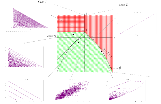
Figure 1. The partition of the parameter space described in Theorem 2. The green region corresponds to $\mathcal{R}$, while the red region corresponds to $\mathcal{T}$. The smaller figures are typical trajectories of the Markov chain $(X_{n})_{n\geq 0}$ for each region of the parameter space. In the all the simulations, we chose $\lambda=1$.

Theorem 1 is a simple consequence of this result. Indeed, in the case of $(a,b)\in\mathcal{R}$, the convergence in law of $\tilde{X}_{n}$ simply derives from the convergence in law of $X_{n}$ since $\tilde{X}_{n}$ is the first coordinate of $X_{n}$. In the transient case, $(a,b)\in\mathcal{T}$ the result in Theorem 1 simply derives from the fact that $||X_{n}||_{1}\to_{n\to\infty}\infty$ almost surely.

The rest of the article is devoted to the proof of Theorem 2. We first focus on the recurrent case in Section 3, then on the transient case in Section 4.

3. Proof of Theorem 2: recurrence

In this section, we prove the recurrence part of Theorem 2. The proof goes by exhibiting three functions satisfying a Foster-Lyapounov drift conditions for different ranges of the parameters $(a,b)$ covering the whole recurrent regime $\mathcal{R}$.

3.1. Foster-Lyapounov drift criteria

Drift criteria are powerful tools that have been introduced by Foster [8], and deeply studied, and popularized, by Meyn and Tweedie [12], among others. These drift criteria allow to prove convergence to the invariant measure of Markov chains and yield explicit rates of convergence. We use here the treatment from Douc, Moulines, Priouret and Soulier [5], which is influenced by Meyn and Tweedie [12], but is more suitable for Markov chains which are irreducible but not strongly irreducible.

A set of states $C\subset\mathbb{N}^{2}$ is called petite [5, Definition 9.4.1], if there exists a state $x_{0}\in\mathbb{N}^{2}$ and a probability distribution $(p_{n})_{n\in\mathbb{N}}$ on $\mathbb{N}$ such that

$$\inf_{x\in C}\sum_{n\in\mathbb{N}}p_{n}P^{n}(x,x_{0})>0,$$

where we recall that $P^{n}(x,x_{0})$ is the $n$-step transition probability from $x$ to $x_{0}$. Since the Markov chain $(X_{n})_{n\geq 0}$ is irreducible, any finite set is petite (take $x_{0}$ to be the accessible state) and any finite union of petite sets is petite [5, Proposition 9.4.5].

Let $V:\mathbb{N}^{2}\to[1,\infty)$ be a function, $\varepsilon\in(0,1]$, $K<\infty$ and $C\subset\mathbb{N}^{2}$ a set of states. We say that the drift condition $D(V,\varepsilon,K,C)$ is satisfied if

$$\Delta V(x):=\mathbb{E}_{x}[V(X_{1})-V(X_{0})]\leq-\varepsilon V(x)+K\boldsymbol{1}_{C}$$

It is easy to see that this condition implies condition $D_{g}(V,\lambda,b,C)$ from [5, Definition 14.1.5], with $\lambda=1-\varepsilon$ and $b=K$.

Proposition 1.

Assume that the drift condition $D(V,\varepsilon,K,C)$ is verified for some $V$, $\varepsilon$, $K$ and $C$ as above and assume that $C$ is petite. Then there exists $\beta>1$ and a probability measure $\pi$ on $\mathbb{N}^{2}$, such that, for every initial state $x\in\mathbb{N}^{2}$,

$$\beta^{n}\times\sum_{y\in\mathbb{N}^{2}}V(y)|\mathbb{P}_{x}(X_{n}=y)-\pi(y)|\to 0,\quad n\to\infty.$$

In particular, for every initial state $x\in\mathbb{N}^{2}$,

$$\beta^{n}d_{TV}(\operatorname{Law}(X_{n}),\pi)\to 0,\quad n\to\infty$$

and $\pi$ is an invariant probability measure for the Markov chain $(X_{n})_{n\geq 0}$.

Proof.

As mentioned in Section 2.2, the Markov chain is irreducible and aperiodic. The first statement then follows by combining parts (ii) and (a) of Theorem 15.1.3 in [5] with the remark preceding Corollary 14.1.6 in [5]. The second statement immediately follows, noting that $V\geq 1$. ∎

We will consider separately the following ranges of the parameters:

$$\mathcal{R}_{1} =\{(a,b)\in\mathbb{R}^{2}:a,b<1\text{ and }a+b<1\}\,,$$

$$\mathcal{R}_{2} =\{a>0\text{ and }a^{2}+4b<0\}\,,$$

$$\mathcal{R}_{3} =\{1\leq a<2\text{ and }{-}1<b<1-a\}\,.$$

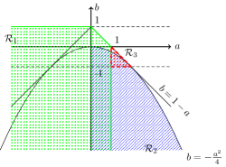
Figure 2. Illustration of the three zones of parameters on which the proof of ergodicity will be carried.

We then have $\mathcal{R}=\mathcal{R}_{1}\cup\mathcal{R}_{2}\cup\mathcal{R}_{3},$ see Figure 2.

3.2. Case $\mathcal{R}_{1}$

Figure 3. Typical trajectory for the case $\mathcal{R}_{1}$. Here, the parameters chosen are $a=0.6,b=0.3$ and $N=1000$

This case is the natural extension of the results that have been already proved for the linear process (see Proposition 1 in [6]).

Let $V:\mathbb{N}^{2}\to\mathbb{R}_{+}$ the function defined by

$$V(i,j):=\alpha i+\beta j+1,$$

where $\alpha,\beta>0$ are parameters to be chosen later.

We then have that $V(i,j)\geq 1$ for all $(i,j)\in\mathbb{N}^{2}$. We look for $\varepsilon>0$ such that $\Delta V(x)+\varepsilon V(x)\leq 0$ except for a finite number of $x\in\mathbb{N}^{2}$.

Let $\varepsilon>0$ to be properly chosen later. Then,

$$\Delta V(i,j)+\varepsilon V(i,j) =\sum_{k\in\mathbb{N}}\dfrac{e^{-s_{ij}}s_{ij}^{k}}{k!}(\alpha k+\beta i+1)-(\alpha i+\beta j+1)+\varepsilon(\alpha i+\beta j+1)$$

$$=\alpha s_{ij}+i(\beta-\alpha+\alpha\varepsilon)+j(\beta\varepsilon-\beta)+\varepsilon\,,$$

Note that $\Delta V+\varepsilon V$ is a linear function of $(i,j)$. We will thus choose $\alpha,\beta$ such that the coefficients of $\Delta V+\varepsilon V$ are negative, so there will be only a finite number of $(i,j)$ that satisfies $\Delta V(i,j)+\varepsilon V(i,j)\geq 0$.

Let us first consider couples $(i,j)$ such that $s_{ij}=0$. According to the above, it is sufficient to have :

$$\left\{\begin{array}[]{ll}\beta-\alpha+\alpha\varepsilon<0\\ \beta\varepsilon-\beta<0\end{array}\right.\Longleftrightarrow\left\{\begin{array}[]{ll}\beta<\alpha(1-\varepsilon)\\ \varepsilon<1\end{array}\right..$$

In the sequel, we impose $\varepsilon<1$.

If $s_{ij}=ai+bj+\lambda>0$, then :

$$\Delta V(i,j)+\varepsilon V(i,j)=i(\alpha a-\alpha+\beta+\alpha\varepsilon)+j(\alpha b+\beta\varepsilon-\beta)+\lambda\alpha+\varepsilon.$$

For the same reasons as before, it is sufficient to have $\alpha,\beta>0$ such that :

$$\left\{\begin{array}[]{ll}\alpha a-\alpha+\beta+\alpha\varepsilon<0\\ \alpha b+\beta\varepsilon-\beta<0\end{array}\right.\Longleftrightarrow\left\{\begin{array}[]{ll}\beta<\alpha(1-a-\varepsilon)\\ \beta>\dfrac{\alpha b}{1-\varepsilon}\hskip 28.45274pt(\mbox{since }\varepsilon<1)\end{array}\right..$$

Let $\alpha:=1$. With the above statements we thus want to choose $\beta,\varepsilon>0$ such that :

$$\left\{\begin{array}[]{ll}\dfrac{b}{1-\varepsilon}<\beta<1-a-\varepsilon\\ \beta<1-\varepsilon\end{array}\right.\hskip 14.22636pt\textit{i.e.}\hskip 14.22636pt\dfrac{b}{1-\varepsilon}<\beta<\min\{1-a-\varepsilon,1-\varepsilon\}.$$

Recall that $a+b<1$, so it is possible to find $\varepsilon_{0}\in(0,1)$ small enough so that :

$$\forall\tilde{\varepsilon}\leq\varepsilon_{0},~{}\dfrac{b}{1-\tilde{\varepsilon}}<1-a-\tilde{\varepsilon}.$$

• If $a\geq 0$, then $\min\{1-a-\varepsilon,1-\varepsilon\}=1-a-\varepsilon$ and since $a<1$, we can choose $\varepsilon\leq\varepsilon_{0}$ so small that $\dfrac{b}{1-\varepsilon}<\beta<\min\{1-a-\varepsilon,1-\varepsilon\}$ on one hand, and $1-a-\varepsilon>0$ on the other hand. It is thus possible to choose $\beta>0$ such that :

  $$\dfrac{b}{1-\varepsilon}<\beta<\min\{1-a-\varepsilon,1-\varepsilon\}.$$

• If $a<0$, then $\min\{1-a-\varepsilon,1-\varepsilon\}=1-\varepsilon$. Since $b<1$, it is possible to set $\varepsilon\leq\varepsilon_{0}$ so small that $b<(1-\varepsilon)^{2}$. Hence we have $\dfrac{b}{1-\varepsilon}<1-\varepsilon$, so that it is possible to choose $\beta>0$ that satisfies our constrains.

Note that $\Delta V(0,0)=\lambda>0$. Hence, with $\alpha,\beta,\varepsilon>0$ chosen as above, we have that :

$$\Delta V(i,j)\leq-\varepsilon V(i,j)\mbox{ except for a finite number of states }(i,j)\in\mathbb{N}^{2}.$$

This proves that a drift condition $D(V,\varepsilon,C)$ holds for $C$ finite set, which yields the result.

3.3. Case $\mathcal{R}_{2}$

In this section, we assume that $a>0$ and $a^{2}+4b<0$.

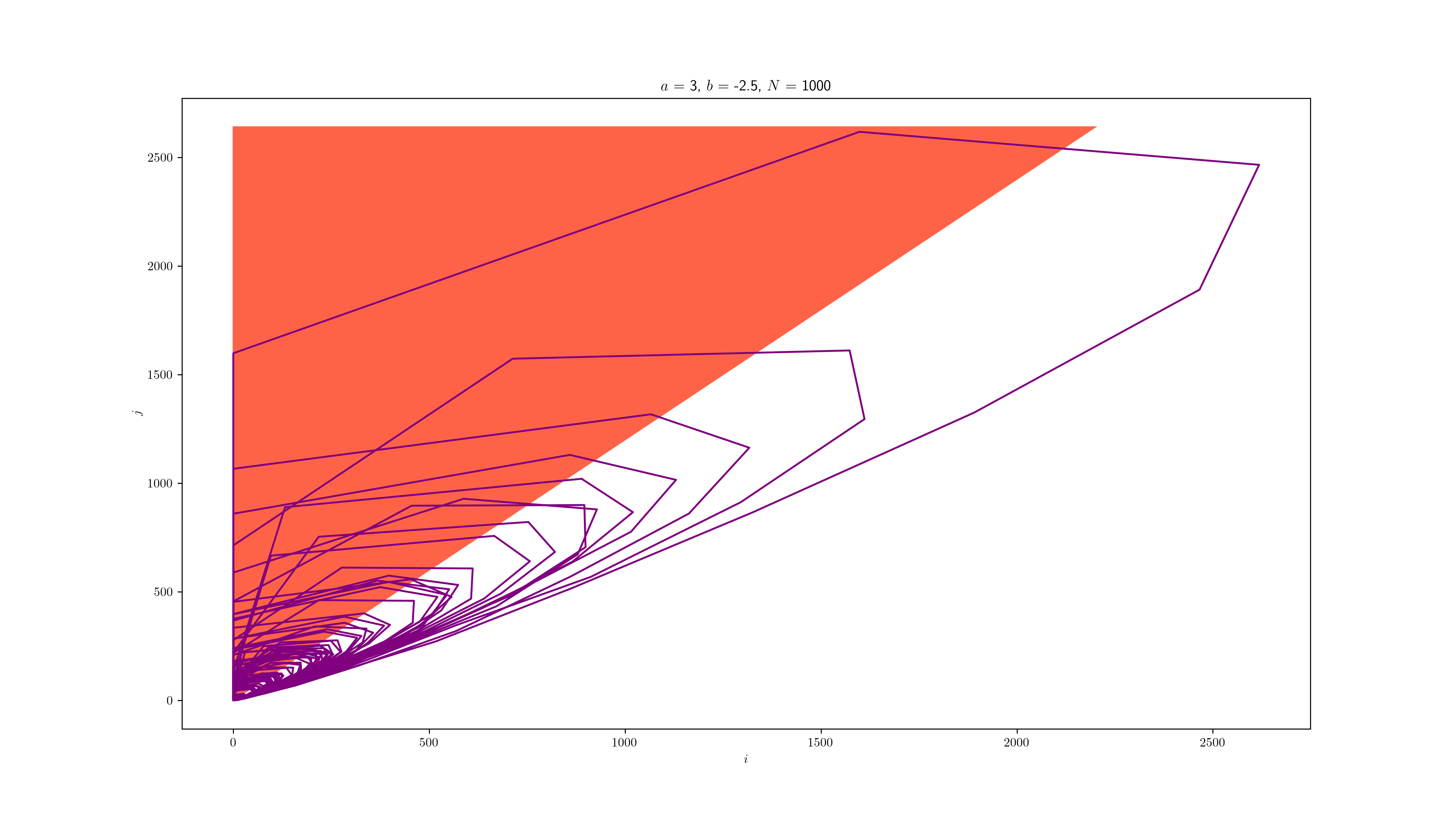
Figure 4. An illustration of Case $\mathcal{R}_{2}$. Here, the parameters are $a=3,b=-2.5$ and $N=1000$. In red, the set $A$ of couples $(i,j)$ such that $s_{ij}=s_{0i}=0$.

The Lyapounov function we will consider is the following one:

$$\forall(i,j)\in\mathbb{N}^{2},\quad V(i,j)=\dfrac{i}{j+1}+1.$$

Before getting into the details, a remark about this function. While we initially discovered it by trial and error, it has an interesting geometric interpretation. As seen in Figure 4, in case $\mathcal{R}_{2}$, the macroscopic trajectories of the Markov chain tend to turn counterclockwise until they hit the $j$-axis and eventually get pulled back to $(0,0)$. This provides a heuristic understanding of why $V$ should be a Lyapounov function. Indeed, it is an increasing function of the angle between the vector $(i,j)$ and the $j$-axis, and therefore $V(X_{n})$ should have a tendency to decrease whenever $X_{n}$ is far away from the $j$-axis.

We now turn to the details. We will need to distinguish the region $A$ of the states $(i,j)$ where $s_{ij}=0$ (shown in red in Figure 4):

$$A:=\left\{(i,j)\in\mathbb{N}^{2}:s_{ij}=0\right\}=\left\{(i,j)\in\mathbb{N}^{2}:ai+bj+\lambda\leq 0\right\}\,.$$ (9)

We have the following lemma:

Lemma 1.

The set $A$ is petite.

Proof.

By definition of $A$, we have $s_{ij}=0$ for all $(i,j)\in A$, hence $P((i,j),(0,i))=1$. Furthermore, for every $i\in\mathbb{N}$, since $b<-a^{2}/4<0$, we have

$$P((0,i),(0,0))=e^{-s_{0i}}=e^{-(\lambda+bi)_{+}}\geq e^{-\lambda}.$$

It follows that

$$\inf_{(i,j)\in A}P^{2}((i,j),(0,0))\geq e^{-\lambda}>0,$$

which shows that $A$ is petite. ∎

Lemma 2.

There exists a finite set $C\subset\mathbb{N}^{2}$ and $\varepsilon\in(0,1)$, such that the drift condition $D(V,\varepsilon,K,A\cup C)$ is satisfied for some $K<\infty$.

Proof.

Since $\dfrac{a^{2}}{4}+b<0$, there exists $\varepsilon\in(0,1)$ small enough such that $\dfrac{a^{2}}{4}+b<b\varepsilon<0$.

Consider $(i,j)\not\in A$, and compute :

$$\Delta V(i,j)+\varepsilon V(i,j)=\dfrac{(\varepsilon-1)i^{2}+bj^{2}+aij+L(i,j)}{(i+1)(j+1)},$$

where $L(i,j)$ is a polynomial of degree 1.

On the numerator we recognize a quadratic form, and as $\frac{a^{2}}{4}+b(1-\varepsilon)<0$, we have that this quadratic form is negative-definite. Thus, there is only a finite number of $(i,j)\not\in A$ such that $\Delta V(i,j)+\varepsilon V(i,j)>0$. We define $C\subset\mathbb{N}^{2}\setminus A$ to be the finite set of such $(i,j)$.

Note that for every $(i,j)\in A$, we have

$$\Delta V(i,j)+\varepsilon V(i,j)\leq\mathbb{E}_{(i,j)}[V(X_{1})]=V(0,i)=1.$$

Hence, setting $K=1\vee\max_{x\in C}\mathbb{E}_{x}[V(X_{1})]\in[1,\infty)$, the finiteness of $K$ following from the fact that $C$ is finite, we have that the drift condition $D(V,\varepsilon,K,A\cup C)$ is satisfied.

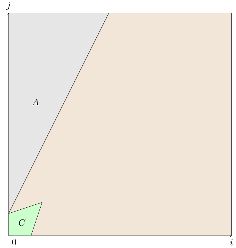
Figure 5. Graphical representation of the sets $A,C$ described above.

Figure 5 illustrates the cutting of the state space that we just described. ∎

In the case $\mathcal{R}_{2}$, by Lemma 1 and Lemma 2, we can now apply Proposition 1. Note that $A\cup C$ is petite because $A$ is petite (Lemma 1), $C$ is finite, hence petite, and the union of two petite sets is again petite. This yields the proof of the case R2 of Theorem 2.

3.4. Case $\mathcal{R}_{3}$

To finish the proof of Theorem 2, it suffices to consider parameters $a$ and $b$ such that $1\leq a<2$ and $-\frac{a^{2}}{4}<b<1-a$. However, for the sake of conciseness, we will prove the ergodicity of the Markov chain on a larger space, namely $\mathcal{R}_{3}$. As a consequence, this case will cover some parameters sets which have already been considered in case $\mathcal{R}_{2}$. Note that this does not represent any issue in our strategy of proof. The choice of $\mathcal{R}_{3}$ will become clearer later on.

We will thus assume here that $1\leq a<2$ and $-1<b<1-a$. Let us denote by $V$ the following function :

$$\forall(i,j)\in\mathbb{N}^{2},\quad V(i,j):=1+\left(i^{2}-aij+\dfrac{b^{2}+1}{2}j^{2}\right)\mathds{1}_{A^{c}}(i,j).$$

First notice that the quadratic form in $V$ is positive-definite.

Indeed, if $1\leq a<2$, then $b^{2}>(1-a)^{2}$ and :

$$4\times\dfrac{b^{2}+1}{2}-a^{2}>2(1-a)^{2}+2-a^{2}=(a-2)^{2}>0.$$

Thus, the function $V$ satisfies $V\geq 1$.

Compute, for $(i,j)\not\in A$ and $\varepsilon\in(0,1)$ to be properly chosen later :

$$\Delta V(i,j)+\varepsilon V(i,j) =\sum_{k=0}^{\infty}\dfrac{e^{-s_{ij}}s_{ij}^{k}}{k!}V(k,i)+(\varepsilon-1)V(i,j)$$

$$\leq\sum_{k=0}^{\infty}\dfrac{e^{-s_{ij}}s_{ij}^{k}}{k!}\left(1+\left(k^{2}-aki+\dfrac{b^{2}+1}{2}i^{2}\right)\right)+(\varepsilon-1)V(i,j)$$

$$=s_{ij}(s_{ij}+1)-ais_{ij}+\dfrac{b^{2}+1}{2}i^{2}+(\varepsilon-1)V(i,j)$$

$$=\left(\dfrac{b^{2}-1}{2}+\varepsilon\right)i^{2}+a(b+1-\varepsilon)ij+\left(\dfrac{b^{2}(1+\varepsilon)+\varepsilon-1}{2}\right)j^{2}+L(i,j),$$

where $L(i,j)$ is a polynomial of degree 1.

We want to choose $\varepsilon\in(0,1)$ such that the above quadratic form is negative-definite, that is, such that :

$$\dfrac{b^{2}-1}{2}+\varepsilon<0,\quad\text{ and }\quad\left(\dfrac{b^{2}-1}{2}+\varepsilon\right)\left(\dfrac{b^{2}(1+\varepsilon)+\varepsilon-1}{2}\right)-\dfrac{a^{2}}{4}(b+1-\varepsilon)^{2}>0.$$ (10)

On the one hand, we have $b^{2}-1<0$. On the other hand, the second inequality in (10) can be written as follows :

$$(b^{2}-1)^{2}-a^{2}(b+1)^{2}+k_{\varepsilon,a,b}>0,$$

where $k_{\varepsilon,a,b}\in\mathbb{R}$ satisfies $k_{\varepsilon,a,b}\underset{\varepsilon\to 0}{\longrightarrow}0$.

In addition, note that :

$$(a,b)\in\mathcal{R}_{3}\Longrightarrow(b^{2}-1)^{2}-a^{2}(b+1)^{2}>0.$$

From the foregoing, we deduce that there exists $\varepsilon\in(0,1)$ small enough such that both conditions of (10) are satisfied. Thus, there is only a finite number of $(i,j)\not\in A$ such that $\Delta V(i,j)+\varepsilon V(i,j)>0$. We define $C\subset\mathbb{N}^{2}\setminus A$ to be the finite set of such $(i,j)$.

Finally, similarly as in Lemma 1, the set $A$ is petite, because $b<1-a\leq 0$. Furthermore similarly as in the case $\mathcal{R}_{2}$, for all $(i,j)\in A$, $\mathbb{E}_{(i,j)}(V(X_{1}))=V(0,i)$ is bounded, since $(0,i)\in A$ except for a finite number of $i$. Since the set $C$ is finite, we have that $A\cup C$ is a petite set and up to an adequate choice of $K$ the drift condition $D(V,\varepsilon,K,A\cup C)$ is satisfied.

4. Proof of Theorem 2: transience

In this section, we show that the Markov chain $(X_{n})_{n\geq 0}$ is transient in the regime $\mathcal{T}$ of the parameters. We will distinguish between the following two cases:

• Case T1 : $a<0,b>1$ (section 4.1).

• Case T2 : $0\leq a<2$ and $a+b>1$ or $a\geq 2$ and $a^{2}+4b>0$ (section 4.2).

In both cases, we will apply the following lemma:

Lemma 3.

Let $S_{1},S_{2},\ldots$ be a sequence of subsets of $\mathbb{N}^{2}$ and $0<m_{1}<m_{2}<\dots$ an increasing sequence of integers. Suppose that

1. On the event $\bigcap_{n\geq 1}\{X_{m_{n}}\in S_{n}\}$, we have $X_{n}\neq(0,0)$ for all $n\geq 1$,

2. $\mathbb{P}_{(0,0)}(X_{m_{1}}\in S_{1})>0$ and for all $n\geq 1$ and every $x\in S_{n}$, we have $\mathbb{P}_{x}(X_{m_{n+1}-m_{n}}\in S_{n+1})>0$.

3. There exist $(p_{n})_{n\geq 1}$ taking values in $[0,1]$ and such that $\sum_{n\geq 1}(1-p_{n})<\infty$, such that

   $$\forall n\geq 1:\forall x\in S_{n}:\mathbb{P}_{x}(X_{m_{n+1}-m_{n}}\in S_{n+1})\geq p_{n}.$$

Then the Markov chain $(X_{n})_{n\geq 0}$ is transient.

Proof.

Since $(0,0)$ is an accessible state, it is enough to show that

$$\mathbb{P}_{(0,0)}(X_{n}\neq(0,0)\,,\forall n\geq 1)>0.$$

Using assumption 1, it is sufficient to prove that

$$\mathbb{P}_{(0,0)}(X_{m_{n}}\in S_{n}\,,\forall n\geq 1)>0.$$ (11)

By assumption 3, there exists $n_{0}\geq 1$ such that $\prod_{n\geq n_{0}}p_{n}>0$. It follows that for every $x\in S_{n_{0}}$,

$$\mathbb{P}_{x}(X_{m_{n}-m_{n_{0}}}\in S_{n}\,,\forall n>n_{0})\geq\prod_{n\geq n_{0}}p_{n}>0.$$

Furthermore, by assumption 2, we have that

$$\mathbb{P}_{(0,0)}(\forall n\leq n_{0}\,,X_{m_{n}}\in S_{n})>0.$$

Combining the last two inequalities yields (11) and finishes the proof. ∎

4.1. Case T1

In this region of parameters, the Markov chain eventually reaches the $i$ and $j$ axes. Indeed, since $a<0$, if $(X_{n})$ hits a state $(i,0)$ with $i\geq-\frac{\lambda}{a}$, as $s_{i0}=(ai+\lambda)_{+}=0$, the next step of the Markov chain will be $(0,i)$. Afterwards, the Markov chain will hits the state $(\mathcal{P}(bi+\lambda),0)$, with $bi+\lambda>i$. Consequently, to follow the example, if we focus on the $i$ axe, starting from $(k,0)$ with $k$ big enough, the Markov chain will return in two steps to a state $(k^{\prime},0)$ belonging to the $i$-axe, satisfying $k^{\prime}>k$ with high probability.

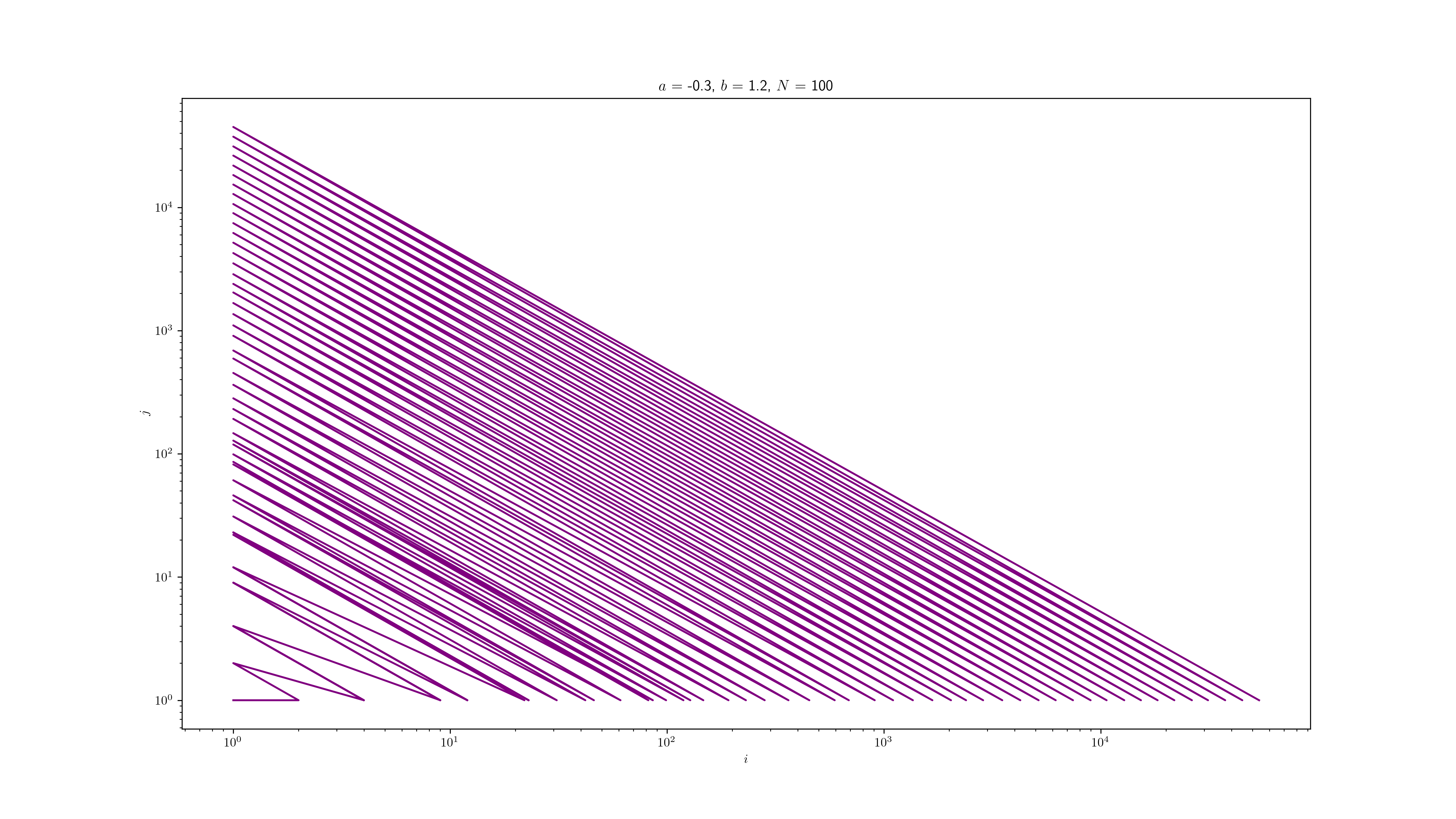
Figure 6. Log-log plot of a typical trajectory of $(X_{n})$, to make the erratic behaviour of the first points of the Markov chain more visible. Here, the parameters are $a=-0.3,b=1.2$ and $N=100$.

In order to formalize these observations, it is very natural to consider the Markov chain induced by the transition matrix $P^{2}$, namely $(X_{2n+1})_{n\geq 0}$. For $i\geq\dfrac{-\lambda}{a},\quad s_{i0}=0$ and thus :

$$\mathbb{P}\left(X_{2n+1}=(k,0)~{}\big{|}~{}X_{2n-1}=(i,0),i\geq\dfrac{-\lambda}{a}\right) =\dfrac{e^{-s_{0i}}s_{0i}^{k}}{k!}$$ (12)

$$=\dfrac{e^{-(bi+\lambda)}(bi+\lambda)^{k}}{k!}.$$

Note that if $a\leq-\lambda$, this results holds for $i\in\mathbb{N}$.

Equation (12) means that if $\tilde{X}_{2n-1}\geq-\frac{\lambda}{a}$, and $\tilde{X}_{2n-2}=0$, then $\tilde{X}_{2n}=0$, and $\tilde{X}_{2n+1}$ is a Poisson random variable with parameter $b\tilde{X}_{2n-1}+\lambda$.

Let us now prove our statement.

Proof of the transience of $(X_{n})$ when $a<0$ and $b>1$.

Fix $r\in(1,b)$. We wish to apply Lemma 3 with

$$m_{n}=2n-1,\quad n\geq 1$$

and

$$S_{n}=\{(i,0)\in\mathbb{N}:i\geq r^{n}\}.$$

We verify that the assumptions (1)-(3) from Lemma 3 hold. For the first assumption, note that if $X_{2n-1}=(i,0)\in S_{n}$, then $X_{2n}=(j,i)$ for some $j$, hence $X_{2n-1}\neq(0,0)$ and $X_{2n}\neq(0,0)$ since $i\geq 1$. In particular, assumption (1) holds.

We now verify that the second assumption holds. For states $x,y\in\mathbb{N}^{2}$, write $x\to_{1}y$ if $\mathbb{P}_{x}(X_{1}=y)>0$. Furthermore, for $S\subset\mathbb{N}^{2}$, write $x\to_{1}S$ if $x\to_{1}y$ for some $y\in S$. Note that $(0,0)\to_{1}(i,0)$ for every $i\in\mathbb{N}$, so that $(0,0)\to_{1}S_{1}$. Now, for every $i\in\mathbb{N}$, we have $(i,0)\to_{1}(0,i)$, and then, because $b>0$, $(0,i)\to_{1}(j,0)$ for every $j\in\mathbb{N}$. In particular, from every $x\in S_{n}$, we can indeed reach $S_{n+1}$ in two steps. Hence, the second assumption is verified as well.

We now prove the third assumption. We claim that there exists $n_{0}\in\mathbb{N}$, such that the following holds:

$$\forall n\geq n_{0},\forall x\in S_{n}:\mathbb{P}_{x}(X_{2}\in S_{n+1})\geq 1-\dfrac{b}{(b-r)^{2}r^{n}}.$$ (13)

To prove (13), first note that according to the earlier remark on (12), if $n_{0}$ is chosen such that $r^{n_{0}}\geq-\lambda/a$, then starting from a state $(i,0)$ with $i\geq r^{n_{0}}$, we have $\tilde{X}_{1}=0$ almost surely and $\tilde{X}_{2}\sim\mathcal{P}(bi+\lambda)$. Therefore, if $n\geq n_{0}$ and $i\geq r^{n}\geq r^{n_{0}}$,

$$1-\mathbb{P}_{(i,0)}(\tilde{X}_{2}\geq r^{n+1},\tilde{X}_{1}=0) =\mathbb{P}_{(i,0)}(\tilde{X}_{2}<r^{n+1})$$

$$\leq\mathbb{P}\left(\mathcal{P}(bi+\lambda)<r^{n+1}\right)$$

$$\leq\mathbb{P}\left(\mathcal{P}(br^{n})<r^{n+1}\right)$$

$$=\mathbb{P}\left(\mathcal{P}(br^{n})-br^{n}<r^{n}(r-b)\right)$$

$$=\mathbb{P}\left(|\mathcal{P}(br^{n})-br^{n}|>r^{n}(b-r)\right)$$

$$\leq\dfrac{b}{(b-r)^{2}r^{n}},$$

by the Bienaymé-Chebychev inequality. This proves (13). Now, (13) implies,

$$\forall x\in S_{n}:\mathbb{P}_{x}(X_{2}\in S_{n+1})\geq p_{n}\coloneqq\left(1-\dfrac{b}{(b-r)^{2}r^{n}}\right)_{+},$$

and

$$\sum_{n\geq 1}(1-p_{n})\leq\sum_{n\geq 1}\dfrac{b}{(b-r)^{2}r^{n}}<\infty.$$

This proves that the third assumption of Lemma 3 holds. The lemma then shows that the Markov chain is transient. ∎

4.2. Case T2: $0\leq a<2$ and $a+b>1$ or $a\geq 2$ and $a^{2}+4b>0$

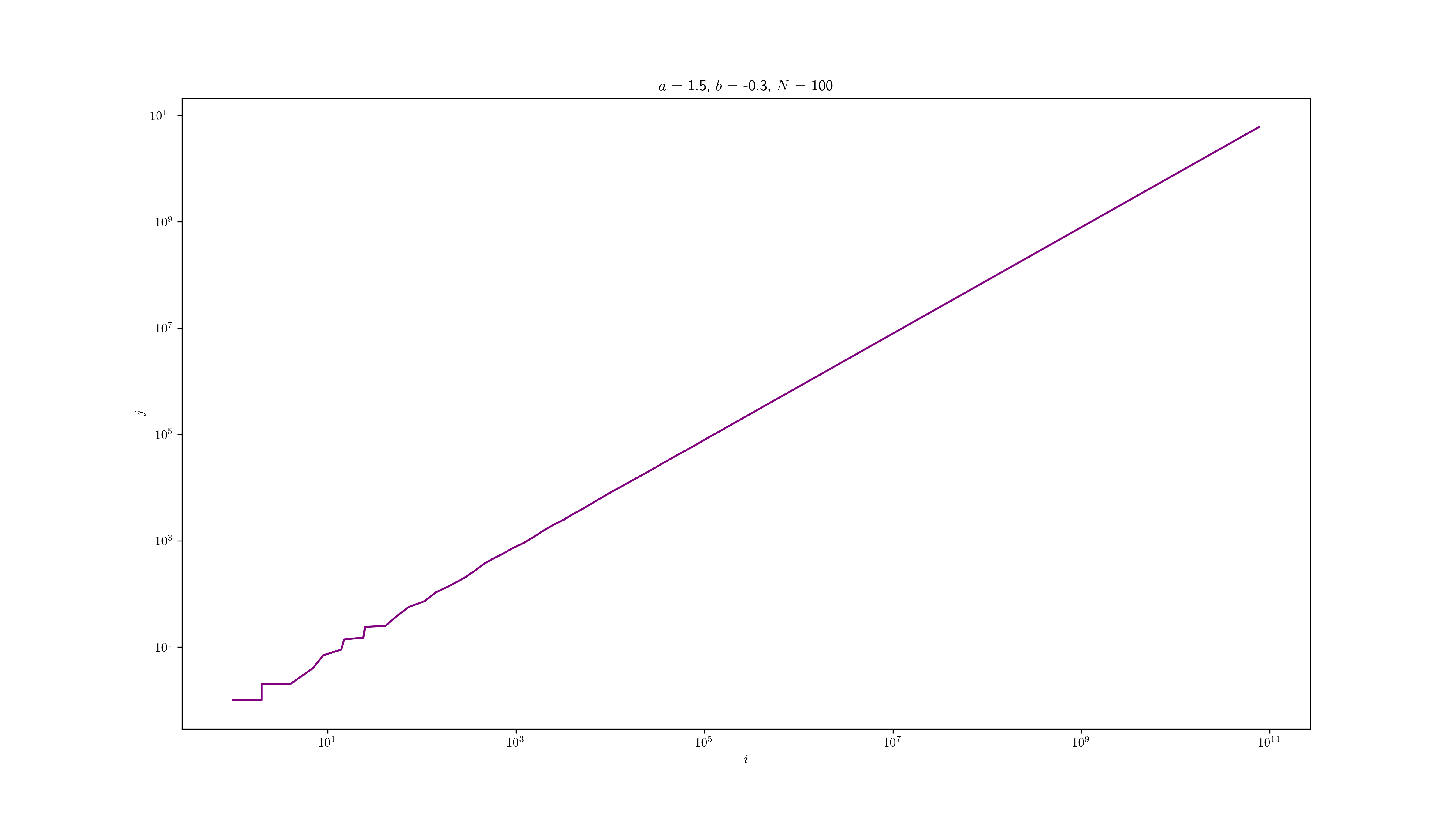
Figure 7. Log-log plot of a typical trajectory of $(X_{n})$, with $a=1.5,b=-0.3$ and $N=100$

For this case, we will take benefit of the comparison between the stochastic process $(\tilde{X}_{n})$ and its linear deterministic version. Namely, let us consider the linear recurrence relation defined by $y_{0},y_{1}\in\mathbb{N}$ and :

$$\forall n\geq 0,\quad y_{n+2}=ay_{n+1}+by_{n}+\lambda.$$ (14)

The solutions to this equation are determined by the eigenvalues and eigenvectors of the matrix $\begin{pmatrix}0&b\\ 1&a\end{pmatrix}$, which is the companion matrix of the polynomial $X^{2}-aX-b$. An eigenvalue of a companion matrix is a root of its associated polynomial. An easy calculation shows that in case T2, we have $a^{2}+4b>0$, hence the eigenvalues are simple and real-valued. We denote the largest eigenvalue by:

$$\theta\coloneqq\dfrac{a+\sqrt{a^{2}+4b}}{2}.$$

The following holds in case T2, as can be easily verified:

$$\theta >1$$ (15)

$$\theta^{2}+b >0.$$ (16)

In fact, one can check that case T2 exactly corresponds to the region in the space of parameters $a,b$ where $\theta>1$, meaning that the sequence $(y_{n+1},y_{n})_{n\geq 0}$, with $(y_{n})_{n\geq 0}$ the solution to (14), grows exponentially inside the positive quadrant, along the direction of the eigenvector $(\theta,1)$.

In what follows, we fix $1<r<\theta$, such that

$$r^{2}-ar-b<0,$$ (17)

where we use the fact that $\theta>1$ is the largest root of the polynomial $X^{2}-aX-b$.

We split our study into two different sub-cases depending on the sign of $b$.

4.2.1. Subcase T2a : $b\geq 0$

In this case, we have $a\tilde{X}_{n}+b\tilde{X}_{n-1}+\lambda>0$ for all $n\in\mathbb{N}$, and so $\tilde{X}_{n+1}\sim\mathcal{P}(a\tilde{X}_{n}+b\tilde{X}_{n-1}+\lambda)$, i.e. no truncation is necessary. It is classical that in this case, $\tilde{X}_{n}$ grows exponentially in $n$ almost surely, but we provide a simple proof for completeness.

We therefore apply Lemma 3 with the sequence $m_{n}=n$ and

$$S_{n}=\{(i,j)\in\mathbb{N}^{2},i\geq r^{n},j\geq r^{n-1}\}.$$

With these notations, assumption 1 is automatically satisfied. Assumption 2 is also satisfied, because $(i,j)\to_{1}(k,i)$ for every $i,j,k\in\mathbb{N}$, since $ai+bj+\lambda>0$ for every $i,j\in\mathbb{N}$ as explained above.

In order to prove assumption 3, let us consider $n\in\mathbb{N}$ and let $(i,j)\in S_{n}$. By definition, starting from $(i,j)$, $\tilde{X}_{1}\sim\mathcal{P}(ai+bj+\lambda)$. Thus,

$$\mathbb{P}_{(i,j)}(\tilde{X}_{1}<r^{n+1}) =\mathbb{P}\left(\mathcal{P}(ai+bj+\lambda)<r^{n+1}\right)$$

$$\leq\mathbb{P}\left(\mathcal{P}(ar^{n}+br^{n-1})<r^{n+1}\right)$$

$$=\mathbb{P}\left(\mathcal{P}(ar^{n}+br^{n-1})-(ar^{n}+br^{n-1})<r^{n-1}(r^{2}-ar-b)\right).$$

Recall that $r^{2}-ar-b<0$ by (17), which implies :

$$\mathbb{P}_{(i,j)}(\tilde{X}_{1}<r^{n+1}) \leq\mathbb{P}\left(\left|\mathcal{P}(ar^{n}+br^{n-1})-(ar^{n}+br^{n-1})\right|>-r^{n-1}(r^{2}-ar-b)\right)$$

$$\leq\dfrac{(a+b)r^{2}}{r^{n}(r^{2}-ar-b)^{2}},$$

where we used again the Bienaymé-Chebychev inequality. Thus

$$\mathbb{P}_{(i,j)}(X_{1}\in S_{n+1})\geq\left(1-\dfrac{(a+b)r^{2}}{r^{n}(r^{2}-ar-b)^{2}}\right)_{+}\eqqcolon p_{n}.$$

This allows to conclude the proof with Lemma 3, as in the previous case.

4.2.2. Subcase T2b : $b<0$

In this case, because of the negativity of $b$ it is more difficult to find an adequate lower-bound of $a\tilde{X}_{n}+b\tilde{X}_{n-1}$. We will thus prove a stronger result, which is illustrated on Figure 7 : asymptotically, the process $(\tilde{X}_{n})$ grows exponentially and the ratio $\tilde{X}_{n+1}/\tilde{X}_{n}$ is close to $\theta$.

From (17) and (16), we can choose $\varepsilon>0$ small enough such that :

$$r^{2}-a(r-\varepsilon)-b<0$$ (18)

$$\theta^{2}-\theta\varepsilon+b>0.$$ (19)

We will use Lemma 3 using $m_{n}=n$ and for $n\in\mathbb{N}^{*}$ :

$$S_{n}=\left\{(i,j)\in\mathbb{N}^{2},i\geq r^{n},j\geq r^{n-1},\left|\frac{i}{j}-\theta\right|\leq\varepsilon\right\}.$$

Note that Assumption 1 from Lemma 3 is again automatically verified. Assumption 2 is also verified, since for $(i,j)\in S_{n}$, we have

$$ai+bj+\lambda>\big{[}a(\theta-\varepsilon)+b\big{]}j\geq\big{[}a(r-\varepsilon)+b\big{]}j>0,$$ (20)

by (18), and so $(i,j)\to_{1}(k,i)$ for every $k\in\mathbb{N}$.

We now show that Assumption 3 from Lemma 3 is verified. Let $n\in\mathbb{N}$ and $(i,j)\in S_{n}$. Then :

$$\mathbb{P}_{(i,j)}(X_{1}\notin S_{n+1}) \leq\mathbb{P}_{(i,j)}\left(\tilde{X}_{1}<r^{n+1}\right)+\mathbb{P}_{(i,j)}\left(\left|\dfrac{\tilde{X}_{1}}{i}-\theta\right|>\varepsilon\right)$$ (21)

We first bound the first term on the right-hand side of (21). By (20), we have

$$\mathbb{P}_{(i,j)}\left(\tilde{X}_{1}<r^{n+1}\right)$$

$$=\mathbb{P}\left(\mathcal{P}(ai+bj+\lambda)<r^{n+1}\right)$$

$$\leq\mathbb{P}\left(\mathcal{P}\Big{(}\big{[}a(r-\varepsilon)+b\big{]}r^{n-1}\Big{)}<r^{n+1}\right)$$

$$=\mathbb{P}\left(\mathcal{P}\Big{(}\big{[}a(r-\varepsilon)+b\big{]}r^{n-1}\Big{)}-\big{[}a(r-\varepsilon)+b\big{]}r^{n-1}<r^{n-1}\big{[}r^{2}-a(r-\varepsilon)-b\big{]}\right).$$

Furthermore, using (18) and applying the Bienaymé-Chebychev inequality we obtain :

$$\mathbb{P}_{(i,j)}\left(\tilde{X}_{1}<r^{n+1}\right)$$ (22)

$$\leq\mathbb{P}\left(\left|\mathcal{P}\Big{(}\big{[}a(r-\varepsilon)+b\big{]}r^{n-1}\Big{)}-\big{[}a(r-\varepsilon)+b\big{]}r^{n-1}\right|>-r^{n-1}\big{[}r^{2}-a(r-\varepsilon)+b\big{]}\right)$$

$$\leq\dfrac{\big{[}a(r-\varepsilon)+b\big{]}r^{n-1}}{\Big{[}r^{n-1}\big{[}r^{2}-a(r-\varepsilon)+b\big{]}\Big{]}^{2}}$$

$$=\dfrac{\big{[}a(r-\varepsilon)+b\big{]}r}{r^{n}\big{[}r^{2}-a(r-\varepsilon)+b\big{]}^{2}}=\dfrac{C_{1}}{r^{n}},$$

where $C_{1}$ is a constant that does not depend on $n$.

We now bound the second term on the right-hand side of (21). Let us write :

$$\left|\dfrac{\tilde{X}_{1}}{i}-\theta\right| =\left|\dfrac{\tilde{X}_{1}-\mathbb{E}_{(i,j)}[\tilde{X}_{1}]}{i}\right|+\left|\dfrac{\mathbb{E}_{(i,j)}[\tilde{X}_{1}]}{i}-\theta\right|$$

First notice that, for any $(i,j)\in S_{n}$ :

$$\left|\dfrac{\mathbb{E}_{(i,j)}\left[\tilde{X}_{1}\right]}{i}-\theta\right| =\left|\dfrac{ai+bj+\lambda}{i}-\theta\right|=\left|a+b\dfrac{j}{i}+\dfrac{\lambda}{i}-\theta\right|$$

$$\leq\underbrace{\left|a+\frac{b}{\theta}-\theta\right|}_{=0}+|b|\left|\dfrac{j}{i}-\frac{1}{\theta}\right|+\frac{\lambda}{i}$$

$$<\dfrac{|b|}{\theta(\theta-\varepsilon)}\varepsilon+\frac{\lambda}{i},$$ (23)

where we used that if $|x-\theta|<\varepsilon$ and $\varepsilon<\theta$, then

$$\left|\frac{1}{x}-\frac{1}{\theta}\right|=\frac{|\theta-x|}{x\theta}<\frac{\varepsilon}{\theta(\theta-\varepsilon)}.$$

To prove that $\mathbb{P}_{(i,j)}\left(\left|\dfrac{\tilde{X}_{1}}{i}-\theta\right|>\varepsilon\right)\leq\dfrac{C_{2}}{r^{n}}$, where $C_{2}$ is a constant that does not depend on $n$, we deduce from (23) that it is sufficient to show that :

$$\mathbb{P}_{(i,j)}\left(\dfrac{\Big{|}\tilde{X}_{1}-\mathbb{E}_{(i,j)}[\tilde{X}_{1}]\Big{|}+\lambda}{i}>\delta\varepsilon\right)\leq\frac{C_{2}}{r^{n}},$$

where, by (19), we have

$$\delta\coloneqq 1-\dfrac{|b|}{\theta(\theta-\varepsilon)}>0.$$

Furthermore, since $b<0$ and $(i,j)\in S_{n}$, we have that

$$ai+bj+\lambda\leq ai+\lambda\leq(a+\lambda)i.$$

We finally have, using the Bienaymé-Chebyshev inequality :

$$\mathbb{P}_{(i,j)}\left(\dfrac{\Big{|}\tilde{X}_{1}-\mathbb{E}_{(i,j)}[\tilde{X}_{1}]\Big{|}+\lambda}{i}>\delta\varepsilon\right) =\mathbb{P}_{(i,j)}\left(\Big{|}\tilde{X}_{1}-\mathbb{E}_{(i,j)}[\tilde{X}_{1}]\Big{|}>\delta\varepsilon i-\lambda\right)$$

$$\leq\dfrac{(a+\lambda)i}{(\delta\varepsilon i-\lambda)^{2}}$$

$$\leq\dfrac{a+\lambda}{\left(\delta\varepsilon r^{n/2}-\lambda r^{-n/2}\right)^{2}}$$

This yields, for some constant $C_{2}<\infty$,

$$\mathbb{P}_{(i,j)}\left(\dfrac{\Big{|}\tilde{X}_{1}-\mathbb{E}_{(i,j)}[\tilde{X}_{1}]\Big{|}+\lambda}{i}>\left(1-\dfrac{|b|}{\theta(\theta-\varepsilon)}\right)\varepsilon\right)\leq\frac{C_{2}}{r^{n}}.$$ (24)

Combining (22) and (24) we have that :

$$\mathbb{P}_{(i,j)}(X_{1}\in S_{n+1})\geq\left(1-\dfrac{C_{1}+C_{2}}{r^{n}}\right)_{+}=:p_{n}.$$

Which will finally lead us to the result, by using Lemma 3 as before.

Appendix A Criteria for strong irreducibility

The Markov chain considered in this article is irreducible in the (weak) sense of Douc, Moulines, Priouret and Soulier [5], but not necessarily strongly irreducible, i.e. irreducible in the classical sense. In this section, we study the decomposition of the state space into communicating classes. We recall the basic definitions. Let $x,y\in\mathbb{N}^{2}$. We say that $x$ leads to $y$, or, in symbols, $x\to y$, if there exists $n\geq 0$ such that $\mathbb{P}(X_{n}=y\mid X_{0}=x)>0$. We say that $x$ communicates with $y$ if $x\to y$ and $y\to x$. This is an equivalence relation which partitions the state space $\mathbb{N}^{2}$ into classes called communicating classes.

Recall that the Markov chain is called strongly irreducible if all states are accessible, equivalently, if $\mathbb{N}^{2}$ is a communicating class. A communicating class $C\subset\mathbb{N}^{2}$ is called closed if there does not exist $x\in C$ and $y\in C^{c}$, such that $x\to y$.

Proposition 2.

• The Markov chain $(X_{n})$ is strongly irreducible on $\mathbb{N}^{2}$ if and only if $a\geq 0$, or if $a>-\lambda$ and $a+b\geq 0$.

• The communicating class of $(0,0)$ contains

  $$\mathcal{S}=\left\{(0,0)\right\}\cup\left\{(0,k),k\in\mathbb{N}^{*}\right\}\cup\left\{(k,0),k\in\mathbb{N}^{*}\right\}.$$ (25)

  and is actually equal to $\mathcal{S}$ iff $a\leq-\lambda$.

We will use the following :

Lemma 4.

Let $i,j,k,\ell\in\mathbb{N}$. The transition matrix $P$ of the Markov chain $(X_{k})$ satisfies :

$$P^{2}\left((i,j),(k,\ell)\right)=\dfrac{e^{-(s_{ij}+s_{\ell i})}s_{ij}^{\ell}s_{\ell i}^{k}}{\ell!~{}k!},$$

and for all $n\geq 3$,

$$P^{n}\left((i,j),(k,\ell)\right)={{\sum}}_{m_{1},\dots,m_{n-2}\in\mathbb{N}}\dfrac{\exp\left\{-\displaystyle\sum_{q=1}^{n}s_{\sigma_{q+1}^{n}\sigma_{q+2}^{n}}\right\}\displaystyle\prod_{q=1}^{n}s_{\sigma_{q+1}^{n}\sigma_{q+2}^{n}}^{\sigma_{q}^{n}}}{m_{1}!\dots m_{n-2}!~{}k!~{}\ell!},$$ (26)

with $\sigma^{n}:=(\sigma^{n}_{1},\sigma^{n}_{2},\dots,\sigma^{n}_{n+2})=(k,\ell,m_{n-2},\dots,m_{1},i,j)$.

Proof of proposition 2.

As mentioned above:

$$(i,j)\to(0,i)\to(0,0),$$

for any $(i,j)\in\mathbb{N}^{2}$ since it only requires that 2 successive 0 are drawn from the Poisson random variable. Therefore, to prove strong irreducibility, it is thus sufficient to prove that $(0,0)\leadsto(i,j)$, for all $(i,j)\in\mathbb{N}^{2}$. Let us consider different cases, depending on the values of the parameters $a$ and $b$.

$-$ If $a\geq 0$ :

Since $\lambda>0,s_{00}>0$ thus $(j,0)$ is accessible from $(0,0)$, for all $j\in\mathbb{N}$.

Moreover, when $a\geq 0$, $s_{j0}=(aj+\lambda)_{+}>0$ and then $(j,0)\to(i,j)$, yielding the result.

$-$ If $-\lambda<a<0$ and $a+b\geq 0$ :

Let $k\in\mathbb{N}$. Since $a+b\geq 0$ and $a+\lambda>0$, we have :

$$s_{k+1,k}=(a(k+1)+bk+\lambda)_{+}=((a+b)k+a+\lambda)_{+}>0,$$

Let $(i,j)\in\mathbb{N}^{2}$. Since $s_{k+1,k}>0$ for all $k$, we deduce that any $(\ell,k+1)$ is accessible from $(k+1,k)$. Thus, in order to reach $(i,j)$ from $(0,0)$, we move from small steps to $(j,j-1)$, and then reach $(i,j)$ :

$$(0,0)\to(1,0)\to(2,1)\to\dots\to(j,j-1)\to(i,j).$$

which concludes the proof of this case.

$-$ If $a\leq-\lambda$:

We will prove that the communicating class of $(0,0)$ is given by (25).
Let $k\in\mathbb{N}^{*}$, then as previously, we have that $(0,0)\to(k,0)$ since $s_{00}>0$, however since $a\leq-\lambda$, $s_{k0}=(ak+\lambda)_{+}=0$, and the next step of the Markov chain will be $(0,k)$. Depending on the value of the parameter $b$, the next step of the Markov chain will either be $(0,0)$ if $s_{0k}=0$, or $(k^{\prime},0)$ with $k^{\prime}\geq 0$ if $s_{0k}>0$ and so on. This proves that the class $cl(0,0)$ is closed and given by (25).

$-$ If $-\lambda<a<0$ and $a+b<0$

In this case we can only prove that the Markov chain is not strongly irreducible on $\mathbb{N}^{2}$ but we do not identify the communicating class of $(0,0)$.

• Case 1 : $b\leq 0$.

  Since $a<0$, we can choose $k_{\star}$ such that

  $$ak_{\star}+\lambda\leq 0.$$

  We will show that it is not possible to reach the state $(1,k_{\star})$. Assuming the opposite leads to the existence of $\ell\in\mathbb{N}$ such that $(k_{\star},\ell)\to(1,k_{\star})$ which implies that $s_{k_{\star},\ell}>0$. If $b>0$, we deduce that necessarly

  $$ak_{\star}+b\ell+\lambda>0\Longrightarrow\ell<\dfrac{-ak_{\star}-\lambda}{b}\leq 0,$$

  so $\ell<0$ which is contradictory. We then deduce that the Markov chain is reducible.

  If $b=0$, $s_{k_{\star},\ell}>0$ would imply that $ak_{\star}+\lambda>0$ which contradicts the definition of $k_{\star}$.

• Case 2 : $b>0$.

  Since $a+b<0$, it is possible to choose $k_{\star}\in\mathbb{N}$ large enough so that :

  $$(a+b)k_{\star}+\lambda\leq 0.$$

  In particular, $0\geq ak_{\star}+bk_{\star}+\lambda\geq ak_{\star}+\lambda$, so that :

  $$\dfrac{-ak_{\star}-\lambda}{b}\geq k_{\star}\geq\dfrac{-\lambda}{a}.$$

  Notice that $k_{\star}\geq 2$ since $k_{\star}\geq\dfrac{-\lambda}{a}>1$.

  We will show that it is not possible to reach $(1,k_{\star})$ starting from $(0,0)$. Assuming the opposite leads us to the existence of $n\in\mathbb{N}$ such that

  $$P^{n}\left((0,0),(1,k_{\star})\right)>0.$$

  Using (26) in the Lemma 4 implies that it exists $m_{1},\dots,m_{n-2}\in\mathbb{N}$ such that :

  $$\left\{\begin{array}[]{ll}s_{k_{\star},m_{n-2}}>0\vspace{0.1cm}\\ s_{m_{n-2}m_{n-3}}^{k_{\star}}>0\vspace{0.1cm}\\ \dots\vspace{0.1cm}\\ s_{m_{2}m_{1}}^{m_{3}}>0\vspace{0.1cm}\\ s_{m_{1}0}^{m_{2}}>0\end{array}\right.$$

  First, we thus have that :

  $$ak_{\star}+bm_{n-2}+\lambda>0\Longrightarrow m_{n-2}>\dfrac{-ak_{\star}-\lambda}{b}\geq k_{\star},$$

  then, since $k_{\star}>0$, we necessarily have $s_{m_{n-2}m_{n-3}}>0$. The consideration on the exponent is important, to avoid the case where $s_{ij}=0$ with an exponent equal to 0. It yields :

  $$am_{n-2}+bm_{n-3}+\lambda>0\Longrightarrow m_{n-3}>\dfrac{-am_{n-2}-\lambda}{b}\geq\dfrac{-ak_{\star}-\lambda}{b}\geq k_{\star}.$$

  We thus have by immediate induction that :

  $$\forall i\in\{1,\dots,n-2\},~{}m_{i}\geq k_{\star}\geq\dfrac{-\lambda}{a}.$$

  Finally, $s_{m_{1},0}>0$ implies $am_{1}+\lambda>0$, which is contradictory.

  We conclude that there is no finite path between $(0,0)$ and $(1,k_{\star})$, so the Markov chain $(N_{k})$ is reducible on $\mathbb{N}^{2}$.

∎

References

• [1] Pierre Bremaud and Laurent Massoulie. Stability of Nonlinear Hawkes Processes. The Annals of Probability, 24(3):1563–1588, 1996. Publisher: Institute of Mathematical Statistics.
• [2] Patrick Cattiaux, Laetitia Colombani, and Manon Costa. Limit theorems for hawkes processes including inhibition. Stochastic Processes and their Applications, 149:404–426, 2022.
• [3] Manon Costa, Carl Graham, Laurence Marsalle, and Viet-Chi Tran. Renewal in Hawkes processes with self-excitation and inhibition. Advances in Applied Probability, 52(3):879–915, September 2020. Publisher: Applied Probability Trust.
• [4] D. J. Daley and D. Vere-Jones. An Introduction to the Theory of Point Processes: Volume I: Elementary Theory and Methods. Springer Science & Business Media, April 2006. Google-Books-ID: 6Sv4BwAAQBAJ.
• [5] Randal Douc, Eric Moulines, Pierre Priouret, and Philippe Soulier. Markov chains. Springer Series in Operations Research and Financial Engineering. Springer, Cham, 2018.
• [6] René Ferland, Alain Latour, and Driss Oraichi. Integer-Valued GARCH Process. Journal of Time Series Analysis, 27(6):923–942, November 2006. Publisher: Wiley-Blackwell.
• [7] Konstantinos Fokianos and Roland Fried. Interventions in INGARCH processes. Journal of Time Series Analysis, 31(3):210–225, 2010. _eprint: https://onlinelibrary.wiley.com/doi/pdf/10.1111/j.1467-9892.2010.00657.x.
• [8] F. G. Foster. On the Stochastic Matrices Associated with Certain Queuing Processes. The Annals of Mathematical Statistics, 24(3):355–360, September 1953. Publisher: Institute of Mathematical Statistics.
• [9] Alan G. Hawkes. Spectra of Some Self-Exciting and Mutually Exciting Point Processes. Biometrika, 58(1):83–90, 1971. Publisher: [Oxford University Press, Biometrika Trust].
• [10] Alan G. Hawkes and David Oakes. A Cluster Process Representation of a Self-Exciting Process. Journal of Applied Probability, 11(3):493–503, 1974. Publisher: Applied Probability Trust.
• [11] Matthias Kirchner. Hawkes and inar ($\infty$) processes. Stochastic Processes and their Applications, 126(8):2494–2525, 2016.
• [12] S. P. Meyn and R. L. Tweedie. Markov Chains and Stochastic Stability. Communications and control engineering series. Cambridge University Press, Cambridge ; New York, 2nd ed edition, 2009.
• [13] Mads Bonde Raad and Eva Löcherbach. Stability for Hawkes processes with inhibition. Electronic Communications in Probability, 25(none):1 – 9, 2020.