Hierarchical DCC-HEAVY Model for High-Dimensional Covariance Matrices

Hierarchical DCC-HEAVY Model for High-Dimensional Covariance Matrices

Abstract

We introduce a new HD DCC-HEAVY class of hierarchical-type factor models for conditional covariance matrices of high-dimensional returns, employing the corresponding realized measures built from higher-frequency data. The modelling approach features sophisticated asymmetric dynamics in covariances coupled with straightforward estimation and forecasting schemes, independent of the cross-sectional dimension of the assets under consideration. Empirical analyses suggest the HD DCC-HEAVY models have a better in-sample fit, and deliver statistically and economically significant out-of-sample gains relative to the standard benchmarks and existing hierarchical factor models. The results are robust under different market conditions.

Keywords: Asymmetric Volatility; DCC-HEAVY; Factor Model; Time-Varying Beta.

1 Introduction

In this paper, we develop a flexible framework, i.e., HD DCC-HEAVY, that accurately captures the latent covariance structure of the high-dimensional asset returns and allows for sophisticated asymmetric dynamics in the covariances, while at the same time keeping the estimation and forecasting straightforward and independent from the cross-sectional dimension of the assets under consideration.

Our methodology relates to the Realized Beta GARCH model of Hansen et al., (2014) and the corresponding extension of Archakov et al., (2020) that introduce the hierarchical-type factor framework based on the realized GARCH model (Hansen et al., (2012)), taking realized measures as direct inputs. In contrast, we model the dynamics of both conditional and RC in a GJR-type spirit (Glosten et al., (1993)). In addition, they focus on modelling the dynamics of daily returns and adopt intra-daily realized measures, leaving the dynamics of the residuals unspecified. Instead, we use monthly returns and construct realized measures via daily data. As such, we estimate and test our model, defining the conditional covariance matrices completely, for much longer sample periods.

Given that no prior study investigates the forecasting ability of the hierarchical-type factor models, we assess the performance of the distinct versions of our model in terms of the factor set and asymmetric dynamics, comparing them with the benchmark cDCC model, the Realized Beta GARCH model (Hansen et al., (2014)), and its 3-FF extension (Archakov et al., (2020)).

To perform empirical evaluations of the models, we utilize the data from a Kenneth French library on the three Fama-French (FF) factors (Fama and French, (1993)), i.e., market risk, size, and value, together with the momentum factor (Carhart, (1997)), coupled with Yahoo Finance time series of the daily and monthly adjusted prices for a selected cross-section of individual assets, including all the stocks that belong to the S&P500 Index during the entire sample period from January 1962 until January 2023, i.e., $T=732$.
Statistical evaluation criteria consist of the in-sample fit and out-of-sample forecast loss functions, i.e., the Euclidean distance (ED) and Frobenius norm (FN). From the economic point of view, we focus on the global minimum variance portfolio (GMVP) optimization as the corresponding weights are determined solely by forecasts of the conditional covariance matrices over the given investment horizon. In this regard, the models are evaluated in terms of the forecasted conditional portfolio volatility. In order to formally determine whether the quality of the forecasts differs significantly across the models, we apply the model confidence set (MCS) procedure of Hansen et al., (2011), which allows us to identify the subset of models that contains the best forecasting model given a pre-specified level of confidence. We also consider some typical features of the implied portfolio allocations, such as portfolio turnover rates and the short-selling proportion. Finally, we examine the economic significance of differences in portfolio volatility via a utility-based framework of Fleming et al., (2001, 2003).

Both the in-sample and forecasting results imply that our HD DCC-HEAVY class of models significantly outperforms the existing hierarchical models of Hansen et al., (2014) and Archakov et al., (2020), as well as the benchmark cDCC model. With regard to the latter, we prove the benefits of employing the higher-frequency data to model conditional covariances of lower-frequency returns. Conversely, the importance of specifying the RC dynamics could explain the poor performance of Realized GARCH-based models (Hansen et al., (2014), Archakov et al., (2020)). We confirm the robustness of our findings under changing market conditions.

The rest of the paper is organized as follows. Section 2 introduces the hierarchical HD DCC-HEAVY models. Section 3 expounds on the estimation scheme, while the forecast formulas are provided in Section 4. Section 5 describes the empirical methodology, details the data used in the paper, and presents the in- and out-of-sample results of empirical exercises. Section 6 concludes.

2 Modelling Framework

Let us define a $K\times 1$ vector of returns related to the set of factors on month $t$ as $r_{t}^{c}$, the corresponding realized covariance (RC) matrix as $RC_{t}^{c}$. In addition, for $i=1,\dots,N$, we consider an individual asset return $r_{i,t}$ and associated realized measure between an individual asset and the set of factors $RC_{i,t}^{c}$.
In this regard, we observe the two types of information sets. ${\cal F}_{t}^{c}$, composed of the variables related to the set of factors, and ${\cal F}_{t}^{c,i}$, which further incorporates the observable information on an individual asset (for $i=1,\dots,N$).

We consider the factor model for an individual asset return:

$$r_{i,t}=\alpha_{i,t}+(\beta_{i,t})^{\prime}r_{t}^{c}+\varepsilon_{i,t};$$ (1)

$$\begin{split}\beta_{i,t}&=\operatorname{Var}(r_{t}^{c}|{\cal F}_{t-1}^{c})^{-1}\operatorname{Cov}(r_{i,t},r_{t}^{c}|{\cal F}_{t-1}^{c,i})\\ &=(\operatorname{diag}(H_{t}^{c})^{1/2}R_{t}^{c}\operatorname{diag}(H_{t}^{c})^{1/2})^{-1}\operatorname{diag}(H_{t}^{c})^{1/2}\rho_{i,t}(h_{i,t})^{1/2}\\ &=(\operatorname{diag}(H_{t}^{c})^{1/2})^{-1}(R_{t}^{c})^{-1}\rho_{i,t}(h_{i,t})^{1/2};\\ \alpha_{i,t}&=\mu_{i}-(\beta_{i,t})^{\prime}\mu^{c},\end{split}$$ (2)

where $r_{i,t}$ is a close-to-close return of an individual asset on month $t$, $r_{t}^{c}$ is a $K\times 1$ vector of returns of $K$ factors, $\alpha_{i,t}$ and $\varepsilon_{i,t}$ are the intercept and idiosyncratic return component related to $r_{i,t}$, respectively, and $\beta_{i,t}$ is a $K\times 1$ vector of asset betas; $\operatorname{diag}(H_{t}^{c})$ is a $K\times K$ diagonal matrix composed of the conditional variances of factors on month $t$, $R_{t}^{c}$ is the corresponding $K\times K$ conditional correlation matrix, while $h_{i,t}$ denotes the conditional variance of an asset $i$ and $\rho_{i,t}$ a $K\times 1$ vector of conditional correlations between an asset and the factors.

Similarly, factor model for N individual asset returns:

$$r_{t}=\alpha_{t}+B_{t}r_{t}^{c}+\varepsilon_{t},$$ (3)

where $r_{t}$ is a $N\times 1$ vector of returns of individual assets on month $t$, $\alpha_{t}$ and $\varepsilon_{t}$ are the corresponding $N\times 1$ vectors of intercepts and idiosyncratic return components, respectively, and $B_{t}$ is a $N\times K$ matrix of asset betas.

It follows readily:

$$\operatorname{Var}(r_{t}|{\cal F}_{t-1}^{c,i})=B_{t}\operatorname{Var}(r_{t}^{c}|{\cal F}_{t-1}^{c})(B_{t})^{\prime}+\Sigma_{t},$$ (4)

with $\Sigma_{t}=\operatorname{E}(\varepsilon_{t}\varepsilon_{t}^{\prime}|{\cal F}_{t-1}^{c,i})$.

To model (1)-(4), we primarily rely on a hierarchical method introduced by Hansen et al., (2014). In particular, ${\cal F}_{t}^{c}$ is adopted to build up the model for the dynamics of the set of factors. Subsequently, conditional on former estimates, we set up the framework for the dynamics between each individual asset and the factors by utilizing ${\cal F}_{t}^{c,i}$. Ultimately, the nonlinear shrinkage method (Ledoit and Wolf, (2017)) is utilized to define the covariances between idiosyncratic return components of the individual assets.

2.1 Marginal Model for a Set of Factors

We initially specify the marginal model for a set of factors by extending the recently introduced DCC-HEAVY model (Bauwens and Xu, (2022)) to allow for sophisticated asymmetric dynamics in the covariance matrices.

In this regard, we decompose a $K\times K$ conditional covariance matrix of $K$ factors, i.e., $\operatorname{E}(r_{t}^{c}r_{t}^{c^{\prime}}|{\cal F}_{t-1}^{c})=H_{t}^{c}$, as:

$$H_{t}^{c}=\operatorname{diag}(h_{t}^{c})^{1/2}R_{t}^{c}\operatorname{diag}(h_{t}^{c})^{1/2},$$ (5)

where $h_{t}^{c}$ is a $K\times 1$ vector of the conditional variances of factors on month $t$ and $R_{t}^{c}$ is the corresponding $K\times K$ conditional correlation matrix, given $\operatorname{E}(\operatorname{diag}(r_{t}^{c}r_{t}^{c^{\prime}})|{\cal F}_{t-1}^{c})=\operatorname{diag}(h_{t}^{c})$ and $\operatorname{E}(u_{t}^{c}u_{t}^{c^{\prime}}|{\cal F}_{t-1}^{c})=R_{t}^{c}$, with $u_{t}^{c}=r_{t}^{c}\odot(h_{t}^{c})^{-1/2}$.
The dynamics of the conditional variances and correlations, allowing for asymmetric effects, are specified as:

$$h_{t}^{c}=w_{h}+A_{h}^{+}v_{t-1}^{c}\odot\operatorname{I}_{t-1}^{+}+A_{h}^{-}v_{t-1}^{c}\odot\operatorname{I}_{t-1}^{-}+B_{h}h_{t-1}^{c},$$ (6)

where $v_{t}^{c}$ is a $K\times 1$ vector of the realized variances of factors on month $t$, $w_{h}$ is a $K\times 1$ positive vector, and $A_{h}^{+},A_{h}^{-}$, and $B_{h}$ are the $K\times K$ diagonal matrices of coefficients with positive diagonal entries less than 1, with $\odot$ denoting the Hadamard (element-wise) product of matrices, $\operatorname{I}_{t}^{+}=[1_{\{r_{1,t}^{c}>0\}},\dots,1_{\{r_{K,t}^{c}>0\}}]^{\prime}$ the indicator vector of the positive monthly returns, and $\operatorname{I}_{t}^{-}=[1_{\{r_{1,t}^{c}\leq 0\}},\dots,1_{\{r_{K,t}^{c}\leq 0\}}]^{\prime}$ the indicator vector of the negative monthly returns.
Correspondingly,

$$R_{t}^{c}=\tilde{R}+\alpha_{R}RL_{t-1}^{c}+\beta_{R}R_{t-1}^{c},$$ (7)

where $RL_{t}^{c}$ is a $K\times K$ realized correlation matrix of the factors on month $t$, and $\alpha_{R}$ and $\beta_{R}$ are non-negative scalar parameters, i.e., $\beta_{R}=0$ if $\alpha_{R}=0$ and $\beta_{R}<1$, with $\tilde{R}=(1-\beta_{R})\overline{R}-\alpha_{R}\overline{P}$, i.e., $\operatorname{E}(u_{t}^{c}u_{t}^{c^{\prime}})=\overline{R}$ and $\operatorname{E}(RL_{t}^{c})=\overline{P}$ set to the empirical counterparts.

Analogously, we decompose a $K\times K$ conditional mean of the realized covariance (RC) matrix of $K$ factors, i.e., $\operatorname{E}(RC_{t}^{c}|{\cal F}_{t-1}^{c})=M_{t}^{c}$, as:

$$M_{t}^{c}=\operatorname{diag}(m_{t}^{c})^{1/2}P_{t}^{c}\operatorname{diag}(m_{t}^{c})^{1/2},$$ (8)

where $m_{t}^{c}$ is a $K\times 1$ vector of the conditional means of realized variances of factors on month $t$ and $P_{t}^{c}$ is the corresponding $K\times K$ conditional mean of realized correlations, i.e., $\operatorname{E}(RL_{t}^{c}|{\cal F}_{t-1}^{c})=P_{t}^{c}$.
The dynamics of the realized variances and correlations, allowing for daily asymmetric effects, are specified as:

$$m_{t}^{c}=w_{m}+A_{m}^{+}v_{t-1}^{c+}+A_{m}^{-}v_{t-1}^{c-}+B_{m}m_{t-1}^{c},$$ (9)

where $v_{t}^{c+}$ and $v_{t}^{c-}$ are the $K\times 1$ vectors of the positive and negative realized semi-variances (Shephard and Sheppard, (2010)) of factors, respectively, $w_{m}$ is a $K\times 1$ positive vector, and $A_{m}^{+},A_{m}^{-}$, and $B_{m}$ are the $K\times K$ diagonal matrices of coefficients with positive diagonal entries below 1.
Specifically, for $i=1,\dots,K$ and $j=1,\dots,m$, $v_{i,t}^{c+}=\sum_{j=1}^{m}(r_{i,j,t}^{c+})^{2}$ and $v_{i,t}^{c-}=\sum_{j=1}^{m}(r_{i,j,t}^{c-})^{2}$, where $r_{i,j,t}^{c+}=r_{i,j,t}^{c}\times 1_{\{r_{i,j,t}^{c}>0\}}$ and $r_{i,j,t}^{c-}=r_{i,j,t}^{c}\times 1_{\{r_{i,j,t}^{c}\leq 0\}}$ denote the positive and negative daily returns, respectively.
Correspondingly,

$$P_{t}^{c}=(1-\alpha_{P}-\beta_{P})\overline{P}+\alpha_{P}RL_{t-1}^{c}+\beta_{R}P_{t-1}^{c},$$ (10)

where $\alpha_{P}$ and $\beta_{P}$ are non-negative scalar parameters, i.e., $\beta_{P}=0$ if $\alpha_{P}=0$ and $\alpha_{P}+\beta_{P}<1$, with $\operatorname{E}(RL_{t}^{c})=\overline{P}$ set to the empirical counterpart.

2.2 Model for Individual Asset Returns

By assuming that the conditional distribution of individual asset returns depends on the factors but not vice versa (Hansen et al., (2014)), the standardized return of each asset is conditionally jointly distributed with ‘degarched’ factors, i.e.,

$$\begin{pmatrix}u_{t}^{c}\\ u_{i,t}\end{pmatrix}|{\cal F}_{t-1}^{c,i}\sim N\left(\begin{pmatrix}0_{K\times 1}\\ 0_{1\times 1}\end{pmatrix},R_{i,t}^{c}\right),$$ (11)

where the $(K+1)\times(K+1)$ joint conditional correlation matrix $R_{i,t}^{c}$ is given by:

$$R_{i,t}^{c}=\begin{pmatrix}R_{t}^{c}&\rho_{i,t}\\ (\rho_{i,t})^{\prime}&1\end{pmatrix},$$ (12)

where $R_{t}^{c}$ and $\rho_{i,t}$ denote the $K\times K$ conditional correlation matrix of factors filtered from a marginal model and $K\times 1$ vector of correlations between an individual asset and the factors on month $t$, respectively.

In accordance to the framework for a set of factors, the dynamics of the conditional and realized variance of an individual asset, allowing for corresponding asymmetric effects are specified as:

$$h_{i,t}=c_{i,h}+a_{i,h}^{+}v_{i,t-1}1_{[r_{i,t-1}>0]}+a_{i,h}^{-}v_{i,t-1}1_{[r_{i,t-1}\leq 0]}+b_{i,h}h_{i,t-1},$$ (13)

where $h_{i,t}$ and $v_{i,t}$ denote the conditional and realized variance of an asset $i$ on month $t$, respectively, and $c_{i,h},a_{i,h}^{+},a_{i,h}^{-}$, and $b_{i,h}$ are non-negative scalar coefficients;

$$m_{i,t}=c_{i,m}+a_{i,m}^{+}v_{i,t-1}^{+}+a_{i,m}^{-}v_{i,t-1}^{-}+b_{i,m}m_{i,t-1},$$ (14)

where $m_{i,t}$, $v_{i,t}^{+}$, and $v_{i,t}^{-}$ denote the conditional mean of the realized variance, positive and negative semi-variance of an asset $i$ on month $t$, respectively, and $c_{i,m},a_{i,m}^{+},a_{i,m}^{-}$, and $b_{i,m}$ are non-negative scalar coefficients.
Finally, to model the vectors of correlations between the returns of an individual asset and the set of factors, we utilize the Fisher transformation, i.e., $\mathbb{F}(\cdot)$, to map each element from a closed interval $(-1,1)$ into $\mathbb{R}$ within the typical HEAVY-type recursions (Noureldin et al., (2012), Bauwens and Xu, (2022)):

$$\mathbb{F}(\rho_{i,t})=\phi_{i,R}+\alpha_{i,R}\mathbb{F}(rl_{i,t-1})+\beta_{i,R}\mathbb{F}(\rho_{i,t-1}),$$ (15)

where $\rho_{i,t}$ and $rl_{i,t}$ denote the $K\times 1$ vectors of conditional and realized correlations of an asset $i$ with factors on month $t$, respectively, and $\phi_{i,R}$, $\alpha_{i,R}$, and $\beta_{i,R}$ are non-negative scalar parameters;

$$\mathbb{F}(p_{i,t})=\phi_{i,P}+\alpha_{i,P}\mathbb{F}(rl_{i,t-1})+\beta_{i,P}\mathbb{F}(p_{i,t-1}),$$ (16)

where $p_{i,t}$ denotes a $K\times 1$ vector of the conditional means of realized correlations of an asset $i$ with factors on month $t$, and $\phi_{i,P}$, $\alpha_{i,P}$, and $\beta_{i,P}$ are non-negative scalar parameters.

2.3 Idiosyncratic Dynamics

Based on formulas (1)–(4), to fully specify the conditional covariance matrices of individual assets, we should define the dynamics of the residuals, i.e., $\operatorname{E}(\varepsilon_{t}\varepsilon_{t}^{\prime}|{\cal F}_{t-1}^{c,i})$.

In line with most of the literature, we treat the assumption of an exact factor model as strict. As such, for the underlying approximate factor model, we propose applying the nonlinear shrinkage method of Ledoit and Wolf, (2017) to the sample covariance matrix of the residuals, which has been proved preferable with respect to both the linear shrinkage of Ledoit and Wolf, (2004) (Ledoit and Wolf, (2017)) and thresholding schemes (De Nard et al., (2021)).
This methodology implies shifting the eigenvalues of the empirical covariance matrix via the out-of-sample optimization of the minimum variance loss function subject to a required return constraint (Engle and Colacito, (2006)).

It follows directly:

$$\begin{split}\hat{\beta}_{i,t}&=(\operatorname{diag}(\hat{H}_{t}^{c})^{1/2})^{-1}(\hat{R}_{t}^{c})^{-1}\hat{\rho}_{i,t}(\hat{h}_{i,t})^{1/2}\end{split}$$ (17)

and

$$\hat{\operatorname{Var}}(r_{t}|{\cal F}_{t-1}^{c,i})=\hat{B}_{t}\hat{\operatorname{Var}}(r_{t}^{c}|{\cal F}_{t-1}^{c})(\hat{B}_{t})^{\prime}=\hat{B}_{t}\hat{H}_{t}^{c}(\hat{B}_{t})^{\prime}+\hat{\Sigma}_{\hat{\varepsilon}},$$ (18)

where matrices $\hat{H}_{t}^{c}$ and $\hat{R}_{t}^{c}$ are filtered from the core model, i.e., (5-10), whereas each conditional variance $\hat{h}_{i,t}$ and the corresponding correlation vector $\hat{\rho}_{i,t}$ are extracted from the individual factor model related to an asset $i$, i.e., (13-16). The nonlinear shrinkage method (Ledoit and Wolf, (2017)) delivers $\hat{\Sigma}_{\hat{\varepsilon}}$.

3 Estimation

The hierarchical structure of the introduced model suggests a convenient step-by-step estimation procedure independent of the cross-sectional dimension of the assets under consideration. As follows, we discuss the quasi-maximum likelihood (QML) estimation scheme and define the corresponding log-likelihood functions (LLF).

Initially, to estimate the core model for a set of factors, we essentially follow the approach of Bauwens and Xu, (2022), by partitioning the parameters of both conditional and realized covariances into the coefficients of the corresponding variance and correlation equations.
In particular, let us define the two parameter sets $\theta_{H}^{c}$ and $\theta_{M}^{c}$ for the conditional and realized covariances of factors, respectively.

Given the hypothesis that the distribution of the ‘degarched’ monthly return vector is multivariate Gaussian (11), the first step consists of estimating the parameters of the conditional variances (6), i.e., $\theta_{H1}^{c}$, and correlations (7), i.e., $\theta_{H2}^{c}$, for the set of factors by maximizing the following QML functions:

$$\begin{split}LLF_{H1}^{c}(\theta_{H1}^{c}|{\cal F}_{t-1}^{c})&=-\frac{1}{2}\sum_{t=1}^{T}\left\{2\log\left|\operatorname{diag}(h_{t}^{c})^{1/2}\right|+u_{t}^{c^{\prime}}u_{t}^{c}\right\};\\ LLF_{H2}^{c}(\theta_{H2}^{c}|\hat{\theta}_{H1}^{c};{\cal F}_{t-1}^{c})&=-\frac{1}{2}\sum_{t=1}^{T}\left\{\log\left|R_{t}^{c}\right|+\hat{u}_{t}^{c^{\prime}}(R_{t}^{c})^{-1}\hat{u}_{t}^{c}\right\},\end{split}$$ (19)

where $\hat{u}_{t}^{c}=r_{t}^{c}\odot(\hat{h}_{t}^{c})^{-1/2}$, with $\hat{h}_{t}^{c}$ defined via $\hat{\theta}_{H1}^{c}$.
Bauwens and Xu, (2022) show that the estimated parameters for conditional correlations (7), i.e., $(\alpha_{R},\beta_{R})$, do not automatically guarantee the PD-ness of $R_{t}^{c}$. As such, we proceed by checking the condition during the numerical maximization of $LLF_{H2}^{c}$.

To specify the dynamics of realized measures, we assume that the probability density function of RC matrices $RC_{t}^{c}$, conditional on the filtration ${\cal F}_{t-1}^{c}$, is Wishart, i.e.,

$$RC_{t}^{c}|{\cal F}_{t-1}^{c}\sim W_{K}(\nu,M_{t}^{c}(\theta_{M}^{c})/\nu),$$ (20)

where $W_{K}(\nu,M_{t}^{c}(\theta_{M})/\nu)$ denotes the $K$-dimensional central Wishart distribution with $\nu\geq K$ degrees of freedom and PD $K\times K$ scale matrix $M_{t}^{c}(\theta_{M}^{c})/\nu$, implying $E(RC_{t}^{c}|{\cal F}_{t-1}^{c})=M_{t}^{c}(\theta_{M}^{c})$.

Correspondingly, we split $\theta_{M}^{c}$ into the parameters for realized variances (9), i.e., $\theta_{M1}^{c}$, and realized correlations (10), i.e., $\theta_{M2}^{c}$. The second-step objective functions for $T$ observations are given by:

$$\begin{split}LLF_{M1}^{c}(\theta_{M1}^{c}|{\cal F}_{t-1}^{c})=&-\frac{\nu}{2}\sum_{t=1}^{T}\left\{2\log\left|L_{t}^{c}\right|+\operatorname{trace}\left[(L_{t}^{c})^{-1}RC_{t}^{c}(L_{t}^{c})^{-1}\right]\right\};\\ LLF_{M2}^{c}(\theta_{M2}^{c}|\hat{\theta}_{M1}^{c};{\cal F}_{t-1}^{c})=&-\frac{\nu}{2}\sum_{t=1}^{T}\left\{\log\left|P_{t}^{c}\right|+\operatorname{trace}\left[((P_{t}^{c})^{-1}-\operatorname{I}_{K})(\hat{L}_{t}^{c})^{-1}RC_{t}^{c}(\hat{L}_{t}^{c})^{-1}\right]\right\},\end{split}$$ (21)

where $\operatorname{I}_{K}$ denotes the identity matrix of order $K$, $L_{t}^{c}=\operatorname{diag}(m_{t}^{c})^{1/2}$, with $\hat{L}_{t}^{c}$ defined via $\hat{\theta}_{M1}^{c}$, and the parameter $\nu$ set equal to 1.

Next, we consider the likelihood contributions for the conditional model of each individual asset return. It follows from the assumptions (11) and (12), the conditional distribution of the standardized monthly asset return:

$$u_{i,t}|u_{t}^{c}\sim N\left((\rho_{i,t})^{\prime}(R_{t}^{c})^{-1}u_{t}^{c},1-(\rho_{i,t})^{\prime}(R_{t}^{c})^{-1}\rho_{i,t}\right).$$ (22)

As such, the underlying LLF with regard to the conditional covariances of an asset $i$

$$\begin{split}LLF_{H_{i}}^{c,i}(\theta_{H_{i}}|{\cal F}_{t-1}^{c,i})=-\frac{1}{2}\sum_{t=1}^{T}\left\{\log\left(h_{i,t}\left(1-(\rho_{i,t})^{\prime}(R_{t}^{c})^{-1}\rho_{i,t}\right)\right)+\frac{(u_{i,t}-(\rho_{i,t})^{\prime}(R_{t}^{c})^{-1}u_{t}^{c})^{2}}{\left(1-(\rho_{i,t})^{\prime}(R_{t}^{c})^{-1}\rho_{i,t}\right)}\right\},\vspace{-1cm}\end{split}$$ (23)

directly follows from:

$$\begin{split}\operatorname{Cov}(r_{i,t},r_{t}^{c}|{\cal F}_{t-1}^{c,i})&=\operatorname{diag}(h_{t}^{c})^{1/2}\rho_{i,t}(h_{i,t})^{1/2};\\ \operatorname{Var}(r_{i,t}|r_{t}^{c},{\cal F}_{t-1}^{c,i})&=h_{i,t}-\frac{(\operatorname{diag}(h_{t}^{c})^{1/2}\rho_{i,t}(h_{i,t})^{1/2})^{\prime}(\operatorname{diag}(h_{t}^{c})^{1/2}\rho_{i,t}(h_{i,t})^{1/2})}{\operatorname{diag}(h_{t}^{c})^{1/2}R_{t}^{c}\operatorname{diag}(h_{t}^{c})^{1/2}}\\ &=h_{i,t}\left(1-(\rho_{i,t})^{\prime}(R_{t}^{c})^{-1}\rho_{i,t}\right);\\ \operatorname{E}(r_{i,t}|r_{t}^{c},{\cal F}_{t-1}^{c,i})&=\mu_{i}+\frac{(\operatorname{diag}(h_{t}^{c})^{1/2}\rho_{i,t}(h_{i,t})^{1/2})^{\prime}}{\operatorname{diag}(h_{t}^{c})^{1/2}R_{t}^{c}\operatorname{diag}(h_{t}^{c})^{1/2}}(r_{t}^{c}-\mu^{c})=\mu_{i}+(h_{i,t})^{1/2}(\rho_{i,t})^{\prime}(R_{t}^{c})^{-1}u_{t}^{c}.\end{split}$$ (24)

To ensure the positivity of the joint conditional correlation matrix $R_{i,t}^{c}$ (12), we must ensure $(\rho_{i,t})^{\prime}(R_{t}^{c})^{-1}\rho_{i,t}<1$ for each $t=1,...,T$ during the estimation (Archakov et al., (2020)).

In analogous fashion as for the conditional correlations (12), we use a partitioning of the realized measures so that, e.g., the $(K+1)\times(K+1)$ joint conditional mean of the realized correlation matrix, i.e., $P_{i,t}^{c}$, is given by:

$$P_{i,t}^{c}=\begin{pmatrix}P_{t}^{c}&p_{i,t}\\ (p_{i,t})^{\prime}&1\end{pmatrix},$$ (25)

where $P_{t}^{c}$ and $p_{i,t}$ denote the $K\times K$ conditional mean of the realized correlation matrix of factors filtered from a marginal model and $K\times 1$ vector of the conditional expectations of correlations between an individual asset and the factors on month $t$, respectively.
In this regard, the QML function reads as:

$$\begin{split}LLF_{M_{i}}^{c,i}(\theta_{M_{i}}|{\cal F}_{t-1}^{c,i})=-\frac{\nu}{2}\sum_{t=1}^{T}\left\{\log\left(m_{i,t}(1-p_{i|c,t})\right)+\frac{v_{i,t}-(rc_{i,t})^{\prime}(RC_{t}^{c})^{-1}rc_{i,t}}{m_{i,t}(1-p_{i|c,t})}\right\},\\ \end{split}$$ (26)

where $m_{i,t}$ denotes the conditional mean of the realized variance of an asset $i$, i.e., $v_{i,t}$, $rc_{i,t}$ is a $K\times 1$ vector of the realized covariances between an asset $i$ and $K$ factors, and $p_{i|c,t}=(p_{i,t})^{\prime}(P_{t}^{c})^{-1}p_{i,t}$. Analogously, we set $\nu$ equal to 1.

In order to estimate the model for the cross-section of $N$ assets, we initially estimate the marginal model for a set of factors followed by the separate estimations of individual models for $i=1,...,N$, conditional on variables obtained via the core model.

Finally, we apply the nonlinear shrinkage of Ledoit and Wolf, (2017) to obtain the conditional covariances of derived residuals, i.e., $\hat{\varepsilon}_{t}=r_{t}-\hat{\alpha}_{t}-\hat{B}_{t}r_{t}^{c}$.

Considering the estimation of the core model, the total number of parameters with respect to $K$ factors is $8K+4$. Given the assumption of diagonal matrices of coefficients for the variance equations, we split the estimation of $8K$ parameters for the variances into $K$ univariate HEAVY models (Shephard and Sheppard, (2010)). Conversely, the model for each individual asset requires the specification of 14 additional parameters. As follows, a total of $8K+4+14N$ coefficients is generated for the cross-sectional dimension of $N$ assets. Importantly, the maximum likelihood (ML) estimation discussed above is independent of both $K$ and $N$.

4 Forecasting

Forecasting the covariance matrices of asset returns is paramount in derivative pricing, asset allocation, and risk management decisions.
In this regard, in our experiments, we focus on the 1-step-ahead predictions of the conditional covariances of monthly returns for the selected cross-section of $N$ individual assets, i.e., $\operatorname{Var}(r_{t+1}|{\cal F}_{t}^{c,i})$, directly computable via:

$$\hat{\operatorname{Var}}(r_{t+1}|{\cal F}_{t}^{c,i})=\hat{B}_{t+1}\hat{\operatorname{Var}}(r_{t+1}^{c}|{\cal F}_{t}^{c})(\hat{B}_{t+1})^{\prime}+\hat{\Sigma}_{\hat{\varepsilon}}=\hat{B}_{t+1}\hat{H}_{t+1}^{c}(\hat{B}_{t+1})^{\prime}+\hat{\Sigma}_{\hat{\varepsilon}},$$ (27)

where $\hat{H}_{t+1}^{c}$ is a $K\times K$ predicted conditional covariance matrix of factors for the month $t+1$ computed via (5)-(10), $\hat{B}_{t+1}$ is a $N\times K$ matrix of predicted asset betas, and $\hat{\Sigma}_{\hat{\varepsilon}}$ is a $N\times N$ conditional covariance matrix of the forecasted residuals.
In particular, for each asset $i$ and time $t+1$:

$$\begin{split}\hat{\beta}_{i,t+1}&=(\operatorname{diag}(\hat{H}_{t+1}^{c})^{1/2})^{-1}(\hat{R}_{t+1}^{c})^{-1}\hat{\rho}_{i,t+1}(\hat{h}_{i,t+1})^{1/2},\end{split}$$ (28)

where $\operatorname{diag}(\hat{H}_{t+1}^{c})$ is a $K\times K$ diagonal matrix composed of the conditional variances of factors for the month $t+1$, $\hat{R}_{t+1}^{c}$ is the corresponding $K\times K$ conditional correlation matrix, $\hat{h}_{i,t+1}$ denotes the predicted conditional variance of an asset $i$, and $\hat{\rho}_{i,t+1}$ a $K\times 1$ vector of the forecasted conditional correlations between an asset $i$ and the factors.

5 Empirical Application

5.1 Data Construction and Description

For the subsequent empirical analyses, we use monthly returns on factors and assets, and construct realized measures of variances and covariances using daily returns observed within each month. In particular, we compute monthly covariance matrices with the corresponding realized analogues with respect to the three Fama-French (FF) factors (Fama and French, (1993)), i.e., market risk, size, and value, together with the momentum factor (Carhart, (1997)), based on the data obtained from a Kenneth French library.

Our model is tested for a selected cross-section of individual assets, consisting of all the stocks that belong to the S&P500 Index during the entire sample period from January 1962 until January 2023, i.e., $N=20$ and $T=732$.
The stock names and tickers are: American Electric Power Company, Inc. (AEP), The Boeing Company (BA), Caterpillar Inc. (CAT), Chevron Corporation (CVX), DTE Energy Company (DTE), Consolidated Edison, Inc. (ED), General Dynamics Corporation (GD), General Electric Company (GE), Honeywell International Inc. (HON), International Business Machines Corporation (IBM), International Paper Company (IP), The Coca-Cola Company (KO), The Kroger Co. (KR), 3M Company (MMM), Altria Group, Inc. (MO), Merck & Co., Inc. (MRK), Marathon Oil Corporation (MRO), Motorola Solutions, Inc. (MSI), The Procter & Gamble Company (PG), and Exxon Mobil Corporation (XOM).
We build the corresponding time series of the monthly and close-to-close daily returns for each asset based on the prices adjusted for dividends and splits available on Yahoo Finance. As a result, the empirical application at the monthly frequency with realized measures built upon daily data allows for estimating and testing the models for a long sample period.

Table 1 reports, for each factor, the time series means and standard deviations of the realized variances (annualized in percentage, i.e., multiplied by 1200), and of their ‘positive’ and ‘negative’ components used to specify the asymmetric dynamics. The last row indicates the average of the time series means and standard deviations of realized correlations between the factors. The same statistics for the individual assets are shown in the Appendix A, i.e., Table A1.

Factor	MKT	SMB	HML	MOM
r${}_{cc}^{2}$	2.51 (5.07)	1.09 (2.78)	1.05 (2.21)	2.25 (9.37)
$RV$	2.65 (5.75)	0.73 (1.34)	0.83 (1.66)	1.49 (3.40)
$P$	1.25 (2.30)	0.34 (0.47)	0.44 (0.93)	0.65 (1.19)
$N$	1.40 (3.73)	0.39 (0.98)	0.39 (0.82)	0.84 (2.40)
$GJR_{P}$	1.12 (2.15)	0.31 (0.49)	0.46 (1.30)	0.66 (1.60)
$GJR_{N}$	1.53 (5.65)	0.42 (1.35)	0.37 (1.19)	0.83 (3.17)
$RL$	–0.10 (0.50)	–0.03 (0.42)	–0.14 (0.44)	0.01 (0.50)

• $r_{cc}^{2}$: squared close-to-close monthly return; $RV$: realized variance; $P$: positive semi-variance; $N$: negative semi-variance; $GJR_{P}$: $RV$ if monthly return is positive, $0$ if negative; $GJR_{N}$: $RV$ if monthly return is negative, $0$ if positive; $RL$: realized correlation, the average of the 3 time series means and sd-s of realized correlations with the other 3 factors.

Table 1: Time series means and standard deviations (between parentheses) of realized variances, their positive and negative decompositions, squared monthly returns, and realized correlations for the 3 FF and MOM factors

Considering the statistics reported in Table 1, the market and momentum factors appear more volatile compared to the size and value factors. Except for the market factor, each average realized variance is only a fraction of the corresponding average squared close-to-close return. The average negative semi-variance ($N$) of each factor, except HML, is larger than the average positive component ($P$). The same applies for the portions of the variances with respect to the signs of monthly returns, i.e., $GJR_{P}$ and $GJR_{N}$. Besides MOM, all the factors have the negative average realized correlation with respect to the others.

The analogous summary measures for the individual assets, i.e., Table A1, generally suggest that the average realized variance exceeds the corresponding average squared close-to-close return. It might not be suprising, given the realized measures obtained via daily returns that account for the overnight information. In contrast to the set of factors, the average positive semi-variance ($P$) is larger than the negative component ($N$). Conversely, the portions of the variances with respect to the negative monthly returns, i.e., $GJR_{N}$, exceed the $GJR_{P}$. Ultimately, the average realized correlations of all the assets with factors lie in a narrow interval, ranging from 0.28 to 0.36, with rather similar standard deviations.

Figures 1-2 show the time series of the realized variances of the market and momentum factors, and the components of their semi-variance decompositions. They illustrate the occurrence of a few clustered extreme values, consistent with periods of the financial turbulence. In both cases, the extreme volatility is largely attributed to the negative semi-variance due to prevailing negative daily returns during the turmoils.

Figure 3 illustrates the time series of the realized correlations between BA and each factor. The patterns of correlations with the three FF factors are comparable, with BA being the mostly correlated with the market factor. On the other hand, the correlations with MOM are more dispersed and volatile.

Figure 1: Annualized realized variances of the market factor and the terms of their decomposition using the signed daily close-to-close returns

Figure 2: Annualized realized variances of the momentum factor and the terms of their decomposition using the signed daily close-to-close returns

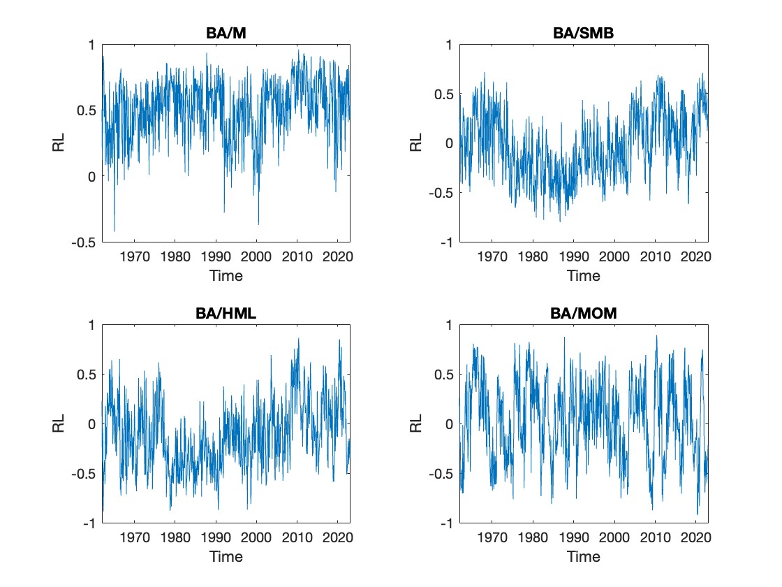
Figure 3: Realized correlations of BA with the three FF factors and MOM

5.2 In-Sample Fit

To evaluate the in-sample fit of our benchmark model, entitled the 4 Factor High-Dimensional DCC-HEAVY (“4F-HD DCC-HEAVY”) model with $K=4$, i.e., 3 FF and momentum factors, we additionally consider the restricted versions with respect to the set of factors and asymmetric effects.

In particular, we estimate the variants by assuming that equity returns are either explained via the 3 FF factors (“FF-HD DCC-HEAVY”) or market factor only (“M-HD DCC-HEAVY”).
In addition, we examine whether allowing for asymmetries in the covariance dynamics allows for improving the fit by specifying the modelling equationns of the benchmark model without accounting for the signs of underlying returns (“sym-HD DCC-HEAVY”).
The corresponding variance equations for “sym-HD DCC-HEAVY” are given by:

$$h_{t}^{c}=w_{h}+A_{h}v_{t-1}^{c}+B_{h}h_{t-1}^{c},$$ (29)

where $v_{t}^{c}$ is a $K\times 1$ vector of the realized variances of factors on month $t$, $w_{h}$ is a $K\times 1$ positive vector, and $A_{h}$ and $B_{h}$ are the $K\times K$ diagonal matrices of coefficients;

$$m_{t}^{c}=w_{m}+A_{m}v_{t-1}^{c}+B_{m}m_{t-1}^{c},$$ (30)

where $m_{t}^{c}$ is a $K\times 1$ vector of the conditional means of realized variances of factors on month $t$, $w_{m}$ is a $K\times 1$ positive vector, and $A_{m}$ and $B_{m}$ are the $K\times K$ diagonal matrices of coefficients;

$$h_{i,t}=c_{i,h}+a_{i,h}v_{i,t-1}+b_{i,h}h_{i,t-1},$$ (31)

where $h_{i,t}$ and $v_{i,t}$ denote the conditional and realized variance of an asset $i$ on month $t$, respectively, and $c_{i,h},a_{i,h}$, and $b_{i,h}$ are non-negative scalar coefficients;

$$m_{i,t}=c_{i,m}+a_{i,m}v_{i,t-1}+b_{i,m}m_{i,t-1},$$ (32)

where $v_{i,t}$ and $m_{i,t}$ denote the realized variance and corresponding conditional mean for an asset $i$ on month $t$, respectively, and $c_{i,m},a_{i,m}$, and $b_{i,m}$ are non-negative scalar coefficients.

Correspondingly, to capture potential additional information provided by the ‘HF’ daily data, we estimate cDCC model built exclusively upon monthly data, which has been widely applied to capture the dynamics of time-varying betas (e.g., Engle and Kelly, (2012), Bali et al., (2017)). In cDCC model, the variance of the market and individual asset is modelled as the benchmark univariate GARCH (Bollerslev, (1986)), while the dynamics of the conditional correlations are specified as:

$$\begin{split}&R_{t}=\operatorname{diag}(Q_{t})^{-1/2}Q_{t}\operatorname{diag}(Q_{t})^{-1/2},\\ Q_{t}=(1-\alpha-\beta)&S+\alpha[\operatorname{diag}(Q_{t-1})^{1/2}u_{t-1}u_{t-1}^{\prime}\operatorname{diag}(Q_{t-1})^{1/2}]+\beta Q_{t-1},\end{split}$$ (33)

where $R_{t}$ denotes the conditional correlation matrix on month $t$, $S$ is a symmetric matrix with unit diagonal elements, $u_{t}=r_{t}\odot(h_{t})^{-1/2}$, with the vector of returns of the market and individual asset $r_{t}=(r_{m,t},r_{i,t})^{\prime}$, coupled with conditional variances $h_{t}=(h_{m,t},h_{i,t})^{\prime}$, and $\alpha$ and $\beta$ are scalar coefficients.

Ultimately, we consider the existing hierarchical factor models including the benchmark Realized Beta GARCH model (Hansen et al., (2014)), coupled with the extended version introduced by Archakov et al., (2020) (“Multivariate Realized Beta GARCH”).

We estimate each model for a cross-section of $N$ selected assets. The in-sample fit of the seven models has been assessed using the three criteria, i.e., the value of the maximized LLF, the Akaike information criterion (AIC), and the Bayesian information criterion (BIC). Given all the models assume that monthly returns are conditionally normal, the LLFs evaluated using only monthly data are directly comparable, i.e., the highest value indicates a superior in-sample fit. Conversely, the lower AIC/BIC values are better. For all the models, we present the average value of each criterion with respect to the $N$ assets.
Table 2 collects the three in-sample fit criteria for each model and comparison. In view of the results obtained, several conclusions can be drawn:

1. The “4F-HD DCC-HEAVY” model has a larger LLF value and correspondingly smaller AIC and BIC than the symmetric version “sym-HD DCC-HEAVY” with respect to both core and conditional models for individual assets. As follows, allowing for the asymmetric dynamics in the covariances of factors, as well as an individual asset vs. the set of factors, based on the signs of underlying daily/monthly returns, improves the in-sample fit of the model.

2. Among the market factor-based models, considering the total LLF values and both information criteria evaluated at the monthly data, the best fitting model is “M-HD DCC-HEAVY”. The relative superiority of our model suggests the benefits of adopting the higher-frequency data to model conditional covariances of lower-frequency returns as opposed to cDCC model. Furthermore, specifying the dynamics of the RC is important as “M-HD DCC-HEAVY” readily outperforms Realized Beta GARCH model of Hansen et al., (2014). The latter provides for a better fit with respect to each criterion compared to the low-frequency data-based cDCC model.

3. The “FF-HD DCC-HEAVY” model outperforms the scalar version of the competing “Multivariate Realized Beta GARCH” of Archakov et al., (2020) in terms of a possible comparison of the conditional LLF for individual assets vs. factors evaluated at the monthly data, thus confirming the advantages of explicitly modelling the dynamics of realized measures.

	4F-HD DCC-HEAVY	sym-HD DCC-HEAVY
LLFc	-17912.52	-18469.61
AIC	49.040	50.551
BIC	49.266	50.752
LLFc,i	-3509.52	-3548.47
AIC	9.627	9.728
BIC	9.715	9.803
LLFc $+$ LLFc,i	-21422.04	-22018.08
AIC	58.667	60.279
BIC	58.981	60.555
	M-HD DCC-HEAVY	Real. Beta GARCH	cDCC
LLF${}_{H}^{c}$ $+$ LLF${}_{H_{i}}^{c,i}$	-3672.63	-3991.02	-4111.86
AIC	10.065	10.943	11.256
BIC	10.134	11.031	11.307
	FF-HD DCC-HEAVY	Mult. Real. Beta GARCH
LLF${}_{H_{i}}^{c,i}$	-1678.84	-1962.60
AIC	4.606	5.384
BIC	4.650	5.434

• LLF^c: total LLF for the core model; LLF^c,i: average (across $N$ assets) total LLF for the conditional model for individual assets;
  LLF${}_{H}^{c}$ $+$ LLF${}_{H_{i}}^{c,i}$: average (across $N$ assets) total LLF evaluated at the monthly data;
  LLF${}_{H_{i}}^{c,i}$: average (across $N$ assets) LLF for the conditional model for individual assets evaluated at the monthly data;
  For each maximum value of the log-likelihood function (LLF), we report the corresponding Akaike (AIC) and Bayesian information criteria (BIC). The values in bold correspond to the best model of each row. The models are estimated using the dataset of 732 observations described in Section 5.1.

Table 2: Maximum log-likelihood function (LLF), AIC and BIC values of estimated models

The estimates of the parameters of the core model for each HD DCC-HEAVY version are reported in Table 3. The results demonstrate that the coefficients in columns III-V noticeably differ for the three models, implying distinct dynamics of the variances of factors.
In each case, the average estimate of the $b_{h}$ parameter is much smaller compared to standard GARCH models, while the average estimates of the $a_{h}^{+}$ and $a_{h}^{-}$ parameters are much larger compared to conventional ARCH terms. In line with the findings of Shephard and Sheppard, (2010), Noureldin et al., (2012), and Bauwens and Xu, (2022), these results suggest that the dynamics of conditional variances are better captured by realized variances than by squared returns. Columns VI-VII present the parameter estimates of the correlations, implying rather responsive series.

Coeff.	$w_{h}$	$a_{h}^{+}$	$a_{h}^{-}$	$b_{h}$	$\alpha_{R}$	$\beta_{R}$
Model
4F-HD DCC-HEAVY	0.000	0.699	0.519	0.495	0.272	0.669
FF-HD DCC-HEAVY	0.000	0.418	0.543	0.518	0.229	0.729
M-HD DCC-HEAVY	0.000	0.286	0.826	0.487	-	-
Coeff.	$w_{m}$	$a_{m}^{+}$	$a_{m}^{-}$	$b_{m}$	$\alpha_{P}$	$\beta_{P}$
Model
4F-HD DCC-HEAVY	0.000	0.140	0.103	0.752	0.249	0.739
FF-HD DCC-HEAVY	0.000	0.061	0.115	0.819	0.221	0.639
M-HD DCC-HEAVY	0.000	0.000	0.135	0.860	-	-

• Presented are the estimates of the parameters that appear in the HD DCC-HEAVY equations of the core model for the conditional variances and correlations (upper panel) and the corresponding realized analogues (lower panel). Columns II-V provide the (average of) estimates of the univariate models for the variance of each factor. Columns VI-VII provide the estimates of the parameters of correlations. Estimation period is January 1962 - December 2022, i.e., $T=732$.

Table 3: Parameter estimates of the core model for HD DCC-HEAVY variants

All the three FF factors exhibit a significant leverage effect with respect to underlying monthly and daily returns, i.e., the greater $a_{h}^{-}$ and $a_{m}^{-}$ parameters compared to $a_{h}^{+}$ and $a_{m}^{+}$, respectively. Thus, one of the main stylized facts of the financial return series, i.e., the stronger impact of negative returns on the volatility, seems incorporated in the dynamics of the FF portfolio returns. The same conclusion no longer holds with the addition of a momentum factor.
In Figure 4, we plot realized variances and correlations for the market and HML factors against fitted conditional variances and correlations via benchmark “4F-HD DCC-HEAVY” model. Clearly, conditional variances track the corresponding realized series closely. In addition, Figure 4 demonstrates a significant temporal variation in the correlation dynamics of selected factors, suggesting the potential importance of defining a time-varying specification for the factor covariances.

Figure 4: Annualized realized and fitted conditional variances of the market and HML factors, and the corresponding correlations

In our empirical analyses, we estimate the conditional models for the cross-section of $N=20$ individual assets (see Section 5.1). The corresponding estimation results for the “FF-HD DCC-HEAVY” model are reported in Table 4.
Again, the effects of the lagged realized variances on the current conditional variances are high, on average. Thus, we confirm the realized measures as more informative about volatility than the squared returns. Correspondingly, the average $a_{i,h}^{-}$ exceeds $a_{i,h}^{+}$, indicating the presence of a leverage effect. Ultimately, the coefficients associated with the dynamics of the realized variances of individual stocks are relatively dispersed, implying distinct dynamics of the corresponding series.

Coeff.	$c_{i,h}$	$a_{i,h}^{+}$	$a_{i,h}^{-}$	$b_{i,h}$	$\phi_{i,R}$	$\alpha_{i,R}$	$\beta_{i,R}$
mean	0.000	0.159	0.222	0.755	0.017	0.022	0.944
min	0.000	0.026	0.082	0.545	0.001	0.001	0.631
1	0.000	0.031	0.085	0.561	0.001	0.001	0.675
5	0.000	0.048	0.097	0.626	0.001	0.001	0.849
10	0.000	0.052	0.099	0.661	0.002	0.002	0.892
25	0.000	0.093	0.144	0.692	0.002	0.002	0.922
50	0.000	0.145	0.213	0.752	0.003	0.002	0.978
75	0.000	0.198	0.278	0.827	0.014	0.014	0.984
90	0.000	0.293	0.305	0.872	0.022	0.026	0.987
95	0.000	0.313	0.442	0.886	0.056	0.082	0.989
99	0.000	0.412	0.458	0.889	0.149	0.236	0.991
max	0.000	0.436	0.462	0.890	0.168	0.275	0.991
Coeff.	$c_{i,m}$	$a_{i,m}^{+}$	$a_{i,m}^{-}$	$b_{i,m}$	$\phi_{i,P}$	$\alpha_{i,P}$	$\beta_{i,P}$
mean	0.000	0.134	0.110	0.751	0.000	0.028	0.819
min	0.000	0.042	0.024	0.603	0.000	0.000	0.611
1	0.000	0.043	0.027	0.611	0.000	0.000	0.616
5	0.000	0.046	0.037	0.632	0.000	0.000	0.636
10	0.000	0.082	0.043	0.653	0.000	0.000	0.689
25	0.000	0.121	0.080	0.687	0.000	0.000	0.745
50	0.000	0.133	0.096	0.748	0.000	0.000	0.844
75	0.000	0.147	0.131	0.803	0.000	0.055	0.905
90	0.000	0.181	0.201	0.853	0.000	0.069	0.931
95	0.000	0.221	0.205	0.869	0.000	0.134	0.940
99	0.000	0.225	0.239	0.914	0.000	0.151	0.941
max	0.000	0.226	0.248	0.925	0.000	0.155	0.941

• Presented are the estimates of the parameters that appear in the “FF-HD DCC-HEAVY” equations of the conditional model for an individual asset, i.e., conditional variances and conditional correlation vectors (upper panel), and the corresponding realized analogues (lower panel). Estimation period is January 1962 - December 2022, i.e., $T=732$.

Table 4: “FF-HD DCC-HEAVY” parameter estimates of the conditional models for individual assets

For HD DCC-HEAVY models, we implicitly assume that the correlations across the selected cross-section of asset returns are explained via either, a single, three, or four sources of the systematic risk, i.e., market, size, value, and momentum. In this regard, the vector of model-implied betas for each asset given by (2) is obtained by accounting for the information from higher- and lower-frequency data.
To present the rich dynamics of estimated betas, we graphically illustrate the “4F-HD DCC-HEAVY” fitted measures for IP in Figure 5. The average market beta is close to 1, implying the IP closely tracks the S&P500 dynamics. Conversely, the means of the value and momentum factors lie in the interval 0.5-0.8, while the average SMB beta is around -0.1. The exposure to the size risk factor varies the most. All the betas hit a range of extreme values during the financial crisis episode. The corresponding summary statistics are given in Table 5.

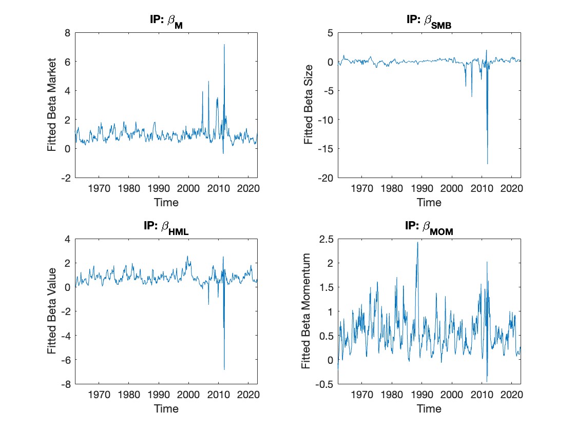
Figure 5: Fitted betas for IP for the period 1962–2022

	$\hat{\beta}_{M}$	$\hat{\beta}_{SMB}$	$\hat{\beta}_{HML}$	$\hat{\beta}_{MOM}$	$\hat{\beta}_{M}$	$\hat{\beta}_{SMB}$	$\hat{\beta}_{HML}$	$\hat{\beta}_{MOM}$
mean	-0.959	-0.116	-0.763	-0.567	-1.433	-0.858	-0.628	-0.794
sd.	-0.541	-0.990	-0.552	-0.378	-1.157	-2.704	-1.181	-0.450
min	-0.369	-17.697	-6.852	-0.466	-0.369	-17.697	-6.852	-0.466
1	-0.273	-2.549	-0.051	-0.015	-0.251	-13.556	-4.387	-0.378
5	-0.414	-0.844	-0.195	-0.100	-0.404	-2.654	-0.648	-0.062
10	-0.499	-0.541	-0.302	-0.145	-0.473	-1.858	-0.302	-0.241
25	-0.645	-0.221	-0.491	-0.299	-0.678	-0.928	-0.507	-0.535
50	-0.886	-0.003	-0.717	-0.514	-1.091	-0.193	-0.690	-0.764
75	-1.122	-0.203	-0.983	-0.763	-1.805	-0.203	-1.066	-1.113
90	-1.426	-0.384	-1.384	-1.008	-3.006	-0.363	-1.483	-1.340
95	-1.705	-0.514	-1.621	-1.296	-3.364	-0.450	-1.671	-1.446
99	-3.190	-0.753	-2.106	-1.755	-5.141	-1.634	-2.273	-1.745
max	-7.185	-2.006	-2.582	-2.433	-7.185	-2.006	-2.536	-2.026

• Presented are the “4F-HD DCC-HEAVY” estimates of betas for IP for the full sample period, i.e., 1962-2022 (left panel), and the financial crisis turbulence, i.e., 2007-2012 (right panel).

Table 5: “4F-HD DCC-HEAVY” beta estimates for IP

5.3 Out-of-Sample Forecasting

We compute the out-of-sample forecasts discussed in Section 4 with regard to all the asymmetric hierarchical-type factor models, which fit the data better compared to the cDCC model, i.e., “4F-HD DCC-HEAVY”, “FF-HD DCC-HEAVY”,“M-HD DCC-HEAVY”, Realized Beta GARCH, and “Multivariate Realized Beta GARCH”.
Starting from the fitting period from January 1962 to December 2016 $(T_{e}=660)$, we generate the forecasts by re-estimating the models every year on a rolling window with $T_{e}$ monthly observations and then producing a sequence of 1-step-ahead predictions based on the updated parameter estimates. We consider the two out-of-sample forecasting periods. The first, characterized by the relatively low volatility of returns, includes the years 2017-2019. The second period lasts until the end of 2022, with the volatility at a relatively high level triggered by the COVID pandemic.

5.3.1 Statistical Accuracy

In order to assess the statistical accuracy of all models, we adopt the two loss functions that produce the consistent ranking (Patton, (2011), Laurent et al., (2013)), i.e., the Euclidean distance (ED) and squared Frobenius norm (FN).
The first is based on the $\operatorname{vech}(\cdot)$ transformation of the forecast error matrix, where the prediction errors on variances and covariances are equally weighted:

$$ED_{t}(C_{t+1},\hat{H}_{t+1})=\operatorname{vech}({C}_{t+1}-\hat{H}_{t+1})^{\prime}\operatorname{I}_{N*}\operatorname{vech}({C}_{t+1}-\hat{H}_{t+1}),$$ (34)

where $\hat{H}_{t+1}$ is the conditional forecast of the covariances of $r_{t+1}$, $C_{t+1}$ is a proxy for the unobserved covariance matrix at time $t+1$, and $\operatorname{I}_{N*}$ is the identity matrix of order $N(N+1)/2$. Indeed, the natural proxy for latent covariances is given by $r_{t}r^{\prime}_{t}$, although others, such as the RC, can be used.
The second loss function is the matrix equivalent of the MSE loss function, where the weights on the covariance forecast errors are doubled compared to the ones on variances:

$$FN_{t}(C_{t+1},\hat{H}_{t+1})=\operatorname{trace}[(C_{t+1}-\hat{H}_{t+1})^{\prime}(C_{t+1}-\hat{H}_{t+1})]=\sum_{i,j}(c_{ij,t+1}-\hat{h}_{ij,t+1})^{2}.$$ (35)

For assessing the significance of differences in the ED and FN losses across the five models, we rely on the model confidence set (MCS) approach of Hansen et al., (2011). The MCS identifies the model or subset of models with the best forecasting performance, given the pre-specified confidence level. It is computed at the 10% significance level using a block bootstrap (Hansen et al., (2003)) with 10,000 replications and the varying block length to verify the robustness of the results.

Table 6 reports the model confidence sets, at the 90% confidence level, using the ED and FN loss functions. The hierarchical models of Hansen et al., (2014) and Archakov et al., (2020) are always excluded from the reported model confidence sets. The “FF-HD DCC-HEAVY” significantly outperforms all the other models during financial turbulence, while during calm times the MCS also incorporates the “M-HD DCC-HEAVY”.

As follows, when all the hierarchical factor models are compared in statistical terms, the new HD DCC-HEAVY models are superior compared to the models built upon the Realized GARCH framework in all cases. Considering the full out-of-sample period, only the “FF-HD DCC-HEAVY” model enters the MCS in terms of both ED and FN losses (Appendix B, Table B1).

Model	ED	MCS 2017-2019	ED	MCS 2020-2022
4F-HD DCC-HEAVY	0.080	0.006	0.828	0.002
FF-HD DCC-HEAVY	0.075	1.000	0.796	1.000
M-HD DCC-HEAVY	0.075	0.885	0.879	0.002
Realized Beta GARCH	0.078	0.091	0.951	0.002
Multivariate Realized Beta GARCH	0.093	0.000	0.954	0.002
Model	FN	MCS 2017-2019	FN	MCS 2020-2022
4F-HD DCC-HEAVY	0.138	0.002	1.340	0.002
FF-HD DCC-HEAVY	0.132	0.320	1.276	1.000
M-HD DCC-HEAVY	0.129	1.000	1.399	0.002
Realized Beta GARCH	0.135	0.008	1.514	0.002
Multivariate Realized Beta GARCH	0.164	0.000	1.527	0.002

• ‘ED/FN’ columns: the average annualized value of ED/FN losses over the corresponding forecast period; bold values identify the minimum loss over the five models.
  ‘MCS 2017-2019’ column: $p$-values of the MCS tests over the out-of-sample period including the years 2017-2019; bold values identify the models included in the MCS at the 90% confidence level (i.e., $p$-values larger than 0.10).
  ‘MCS 2020-2022’ column: the analogous results for the period 2020-2022.

Table 6: Model confidence sets at 90% level of hierarchical factor models, with ED and FN loss functions

5.3.2 Economic Performance

In order to perform the economic evaluation of the forecasting performance we rely on the global minimum variance portfolio (GMVP) optimization (e.g., Engle and Kelly, (2012), Bauwens and Xu, (2022)) since it does not require the estimation of expected returns, providing an essentially clean framework for assessing the merits of distinct covariance forecasting models.

Given a covariance matrix forecast $\hat{H}_{t+1}$, the portfolio weights $\hat{\omega}_{t+1}$ are obtained by solving the minimization problem:

$$\underset{\omega_{t+1}}{\min}\hskip 2.84544pt\omega_{t+1}^{\prime}\hat{H}_{t+1}\omega_{t+1}\quad\operatorname{s.t.}\quad\omega_{t+1}^{\prime}\textbf{1}=1,$$ (36)

where 1 is a $\textit{N}\times 1$ vector of ones.
It follows readily that the optimal GMVP weights are given by:

$$\hat{\omega}_{t+1}=\frac{\hat{H}_{t+1}^{-1}\textbf{1}}{\textbf{1}^{\prime}\hat{H}_{t+1}^{-1}\textbf{1}}.$$ (37)

In addition, we consider the optimization under a short-selling restriction and compute the weights via numerical optimization, i.e., MATLAB Financial Toolbox, given the absence of a closed-form analytical solution. The results are available in Appendix B (Table B3). Given the main aim to assess the accuracy of distinct covariance matrix estimators, our performance measures do not take into account transaction costs.

Initially, we adopt the MCS to select the best-performing models that minimize the standard deviation (SD) of the portfolios obtained by applying the computed weights to the observed returns.

The results presented in Table 7 show that the “M-HD DCC-HEAVY” model provides for the lowest out-of-sample SD during the calm periods, whereas only the “4F-HD DCC-HEAVY” enters the MCS when the volatility is at a relatively high level. Considering the entire out-of-sample period, the MCS includes only the “4F-HD DCC-HEAVY” model (Appendix B, Table B2), while the analogous conclusion applies for long-only portfolios (Appendix B, Table B3). Therefore, in contrast to the statistical performance where the “FF-HD DCC-HEAVY” model is superior, the “4F-HD DCC-HEAVY” appears preferable from a variance minimization perspective.
In general, the “M-HD DCC-HEAVY” model outperforms the competing market factor-based Realized Beta GARCH of Hansen et al., (2014) in all cases. The same applies for a corresponding comparison between the three-factor “FF-HD DCC-HEAVY” and “Multivariate Realized Beta GARCH” (Archakov et al., (2020)) model (Table 7, B2, B3).

Model	SD	MCS 2017-2019	SD	MCS 2020-2022
4F-HD DCC-HEAVY	0.653	0.098	0.571	1.000
FF-HD DCC-HEAVY	0.715	0.000	0.709	0.088
M-HD DCC-HEAVY	0.565	1.000	0.952	0.000
Realized Beta GARCH	0.643	0.098	0.878	0.000
Multivariate Realized Beta GARCH	0.723	0.000	0.718	0.067

• ‘SD’ columns: the average annualized standard deviation of GMVP returns over the corresponding forecast period; bold values identify the minimum loss over the five models.
  ‘MCS 2017-2019’ column: $p$-values of the MCS tests over the out-of-sample period including the years 2017-2019; bold values identify the models included in the MCS at the 90% confidence level (i.e., $p$-values larger than 0.10).
  ‘MCS 2020-2022’ column: the analogous results for the period 2020-2022.

Table 7: Model confidence sets at 90% level of hierarchical factor models, with GMVP loss function

In addition, we examine some basic features of the portfolios, including the Average Return (AR), i.e., the average of out-of-sample returns for the corresponding period, Information Ratio (IR), i.e., the ratio AR/SD, portfolio turnover rates (TO), and proportion of short positions (SP).
The latter are specified as follows:

$$TO_{t}=\sum_{i}^{N}\left\lvert\hat{w}_{i,t}-\hat{w}_{i,t-1}\frac{1+r_{t-1}^{i}}{1+r_{t-1}^{p}}\right\rvert;$$ (38)

$$SP_{t}=\sum_{i}^{N}\mathmybb{1}_{\{\hat{w}_{i,t}<0\}},$$ (39)

where $r_{t}^{p}$ is the total return of the portfolio for the month $t$, $\hat{w}_{i,t}$ and $r_{t}^{i}$ are the weight and return of stock $i$, respectively, and $\mathmybb{1}_{\{\cdot\}}$ denotes the indicator function.

The results reported in Table B4 again confirm that hierarchical HD DCC-HEAVY models consistently and notably outperform Realized GARCH variants. In particular, the “M-HD DCC-HEAVY” features the highest IR during the turbulent periods and overall. On the other hand, the findings summarized in Table B5 suggest that the propensity of models with respect to short positions is very similar and, in general, moderately increases for HD DCC-HEAVY models during turmoils. The increasing trend of the average monthly turnover rates for all models is also visible.

Given that the GMVPs aim at minimizing the variance, and thus the SD, rather than maximizing the expected returns or the IR, the most important performance measure is the out-of-sample SD. In this regard, the out-of-sample returns and IR are also beneficial but should be considered of secondary importance.

Finally, to assess the economic gains of utilizing distinct HD DCC-HEAVY covariance matrix estimators, following Fleming et al., (2001, 2003), we determine the maximum performance fee a risk-averse investor would be willing to pay to switch from using one model to another. Accordingly, we assume that the investor has quadratic preferences of the form:

$$U(r_{t}^{p})=1+r_{t}^{p}-\frac{\gamma}{2(1+\gamma)}(1+r_{t}^{p})^{2},$$ (40)

where $r_{t}^{p}$ is the portfolio return and $\gamma$ is the investor’s relative risk aversion, taking values 1 and 10 (Fleming et al., (2003)). As follows, we determine a fee $\Delta_{\gamma}$ by equating the average realized utilities from two alternative portfolios:

$$\sum_{t=1}^{T}{U(r_{t}^{p_{1}})}=\sum_{t=1}^{T}{U(r_{t}^{p_{2}}-\Delta_{\gamma})},$$ (41)

where $r_{t}^{p_{1}}$ and $r_{t}^{p_{2}}$ are the portfolio returns related to competing HD DCC-HEAVY forecasting strategies.

Major observations based on results in Table 8 are as follows. First, by utilizing the “4F-HD DCC-HEAVY” covariance forecasts, a risk-averse investor can achieve notable economic gains that become pronounced during the crisis period. Overall, an investor with low (high) risk aversion would be willing to pay on average 27 (38) bps to switch from the “FF-HD DCC-HEAVY” strategy to the “4F-HD DCC-HEAVY” and 15 (35) bps for switching from the “M-HD DCC-HEAVY”. These results provide further support that the “4F-HD DCC-HEAVY” might be a preferable hierarchical factor model from the investor point of view.

Period	2017-2019		2020-2022		2017-2022
Model	$\Delta_{1}$	$\Delta_{10}$	$\Delta_{1}$	$\Delta_{10}$	$\Delta_{1}$	$\Delta_{10}$
FF-HD DCC-HEAVY	-6.92	-6.92	61.52	83.84	27.30	38.46
M-HD DCC-HEAVY	28.74	28.74	0.46	40.64	14.60	34.69

• ‘$\Delta_{\gamma}$’ columns: the basis points fee an investor with quadratic utility and relative risk aversion $\gamma$ would pay to switch from the covariance matrix estimator indicated in column 1 to the “4F-HD DCC-HEAVY” model over the period indicated in row 1.

Table 8: BPS fees for switching from simpler HD DCC-HEAVY to the “4F-HD DCC-HEAVY” covariance matrix forecasts

6 Conclusion

In this paper we introduce a class of models for high-dimensional covariance matrices by combining the hierarchical approach of Hansen et al., (2014) and dynamic conditional correlation formulation of a HEAVY model (Noureldin et al., (2012)) recently proposed by Bauwens and Xu, (2022)). In this regard, we rely on the evidence to adopt the higher-frequency data to model more accurate realized measures of covariances and employ them to forecast the conditional covariance matrix of lower-frequency returns (i.e., Noureldin et al., (2012), Gorgi et al., (2019), Bauwens and Xu, (2022)).

An illustrative empirical study for the S&P500 constituents over the period from January 1962 until January 2023, i.e., $N=20$ and $T=732$, shows that our method always significantly outperforms the benchmark and existing hierarchical factor models in statistical and economic terms. The findings are robustified under distinct market conditions.

Avenues for future research are twofold. First, a promising feature of the framework is the ability to readily extract inherently time-varying factor loadings for a given asset or portfolio, thus conforming to the extensive literature that proves the dynamic nature of betas (e.g., Bollerslev et al., (1988), Jagannathan and Wang, (1996), etc.) but also potentially improving the commonly adopted rolling regression approach for their estimation. Second, to verify the relevance of adopted factors, and thus adopt the optimal HD DCC-HEAVY model, the asymptotic theory on estimated loadings and corresponding testing procedures should be derived.

Appendices

A Summary Statistics of for Individual Assets

	r${}_{cc}^{2}$	$RV$	$P$	$N$	$GJR_{P}$	$GJR_{N}$	$RL$
AEP	3.68   (6.54)	4.34   (9.99)	2.21   (4.69)	2.13   (5.55)	1.97   (3.47)	2.37   (9.85)	0.30 (0.21)
BA	11.32 (26.15)	11.54 (19.78)	6.04   (8.81)	5.50 (12.40)	5.69   (9.58)	5.85 (19.13)	0.34 (0.22)
CAT	8.53 (17.46)	8.76 (10.13)	4.43   (4.75)	4.33   (6.71)	4.61   (7.31)	4.15   (9.35)	0.35 (0.23)
CVX	5.27 (10.15)	6.63 (12.97)	3.38   (5.72)	3.25   (8.01)	3.18   (5.45)	3.45 (12.67)	0.34 (0.23)
DTE	3.26   (8.77)	3.96   (7.89)	2.04   (3.97)	1.92   (4.55)	1.97   (4.17)	1.99   (7.26)	0.31 (0.21)
ED	4.40 (26.05)	4.03 (11.62)	1.93   (3.92)	2.10   (9.68)	1.92   (4.17)	2.11 (11.22)	0.30 (0.22)
GD	9.45 (16.93)	9.23   (9.68)	4.94   (5.89)	4.29   (5.42)	4.99   (8.33)	4.24   (8.16)	0.34 (0.22)
GE	6.62 (13.82)	7.52 (12.06)	3.83   (5.71)	3.69   (7.23)	3.35   (6.91)	4.17 (11.21)	0.33 (0.24)
HON	7.53 (18.62)	8.55 (14.84)	4.36   (6.91)	4.19   (9.34)	4.15   (7.29)	4.40 (14.27)	0.36 (0.23)
IBM	5.77 (11.11)	6.39   (8.69)	3.24   (4.12)	3.15   (5.86)	2.92   (4.98)	3.47   (8.43)	0.30 (0.24)
IP	8.44 (22.52)	9.31 (16.22)	4.71   (8.55)	4.60   (9.46)	4.58 (11.59)	4.73 (13.12)	0.35 (0.23)
KO	4.33   (9.19)	5.37   (9.22)	2.77   (4.01)	2.60   (5.74)	2.66   (4.05)	2.71   (9.11)	0.28 (0.23)
KR	7.33 (14.14)	8.42 (10.08)	4.26   (5.36)	4.16   (6.96)	4.34   (7.21)	4.08   (9.22)	0.31 (0.20)
MMM	4.51   (8.47)	5.38   (6.69)	2.72   (3.13)	2.66   (4.52)	2.53   (6.11)	2.85   (4.68)	0.32 (0.24)
MO	6.29 (11.74)	6.63   (8.01)	3.35   (3.95)	3.28   (5.59)	3.43   (5.08)	3.20   (7.76)	0.29 (0.23)
MRK	5.59   (9.53)	6.26   (7.79)	3.17   (3.58)	3.09   (5.79)	3.21   (4.97)	3.05   (7.45)	0.28 (0.22)
MRO	12.67 (46.27)	12.92 (32.01)	6.27 (10.28)	6.65 (24.93)	5.89 (11.51)	7.03 (31.22)	0.35 (0.23)
MSI	11.54 (20.10)	13.72 (17.49)	6.87   (8.08)	6.85 (11.45)	6.56 (10.94)	7.16 (16.74)	0.32 (0.23)
PG	3.73 (10.02)	4.70 (11.17)	2.32   (3.71)	2.38   (8.44)	2.14   (3.52)	2.56 (11.11)	0.28 (0.22)
XOM	3.63   (7.75)	5.28 (10.27)	2.71   (4.72)	2.57   (6.06)	2.51   (4.27)	2.77 (10.05)	0.33 (0.24)

• $r_{cc}^{2}$: squared close-to-close monthly return; $RV$: realized variance; $P$: positive semi-variance; $N$: negative semi-variance; $GJR_{P}$: $RV$ if monthly return is positive, $0$ if negative; $GJR_{N}$: $RV$ if monthly return is negative, $0$ if positive; $RL$: realized correlation, the average of the 4 time series means and sd-s of realized correlations with the set of factors.

Table A1: Time series means and standard deviations (between parentheses) of realized variances, their positive and negative decompositions, squared monthly returns, and realized correlations for the individual assets

B Out-of-Sample Performance cont’d

Model	ED	MCS 2017-2022	FN	MCS 2017-2022
4F-HD DCC-HEAVY	0.454	0.005	0.739	0.003
FF-HD DCC-HEAVY	0.435	1.000	0.704	1.000
M-HD DCC-HEAVY	0.477	0.005	0.764	0.003
Realized Beta GARCH	0.515	0.005	0.824	0.003
Multivariate Realized Beta GARCH	0.524	0.005	0.845	0.003

• ‘ED/FN’ column: the average annualized value of ED/FN losses over the full forecast period; bold values identify the minimum loss over the five models.
  ‘MCS 2017-2022’ columns: $p$-values of the MCS tests over the out-of-sample period including the years 2017-2022; bold values identify the models included in the MCS at the 90% confidence level (i.e., $p$-values larger than 0.10).
  

Table B1: Model confidence sets at 90% level of hierarchical factor models, with ED and FN loss functions over the full out-of-sample period

Model	SD	MCS 2017-2022
4F-HD DCC-HEAVY	0.612	1.000
FF-HD DCC-HEAVY	0.712	0.027
M-HD DCC-HEAVY	0.758	0.005
Realized Beta GARCH	0.761	0.005
Multivariate Realized Beta GARCH	0.720	0.005

• ‘SD’ column: the average annualized standard deviation of GMVP returns over the full forecast period; bold values identify the minimum loss over the five models.
  ‘MCS 2017-2022’ column: $p$-values of the MCS tests over the out-of-sample period including the years 2017-2022; bold values identify the models included in the MCS at the 90% confidence level (i.e., $p$-values larger than 0.10).
  

Table B2: Model confidence set at 90% level of hierarchical factor models, with GMVP loss function over the full out-of-sample period

Period	2017-2019		2020-2022		2017-2022
Model	SD	MCS	SD	MCS	SD	MCS
4F-HD DCC-HEAVY	0.105	0.079	0.137	1.000	0.121	1.000
FF-HD DCC-HEAVY	0.115	0.000	0.144	0.659	0.130	0.000
M-HD DCC-HEAVY	0.112	0.079	0.153	0.659	0.132	0.000
Realized Beta GARCH	0.157	0.000	0.242	0.000	0.199	0.000
Multivariate Realized Beta GARCH	0.080	1.000	0.199	0.091	0.140	0.000

• ‘SD’ columns: the average annualized standard deviation of GMVP returns with short sale restrictions over the forecast period indicated in row 1; bold values identify the minimum loss over the five models.
  ‘MCS’ columns: $p$-values of the MCS tests over the out-of-sample period indicated in row 1; bold values identify the models included in the MCS at the 90% confidence level (i.e., $p$-values larger than 0.10).
  

Table B3: Model confidence set at 90% level of hierarchical factor models, with GMVP loss function under long-only portfolios

Period	2017-2019		2020-2022		2017-2022
Model	AR	IR	AR	IR	AR	IR
4F-HD DCC-HEAVY	0.099	0.937	0.145	1.066	0.122	1.010
FF-HD DCC-HEAVY	0.121	1.051	0.086	0.596	0.104	0.798
M-HD DCC-HEAVY	0.105	0.935	0.221	1.449	0.163	1.231
Realized Beta GARCH	0.027	0.173	0.005	0.020	0.016	0.080
Multivariate Realized Beta GARCH	0.005	0.059	0.116	0.579	0.060	0.431

• ‘AR’ columns: the average annualized GMVP return over the forecast period indicated in row 1.
  ‘IR’ columns: the average annualized AR/SD ratio over the forecast period indicated in row 1.
  

Table B4: Alternative economic performance measures for hierarchical factor models based on GMVP optimization

Period	2017-2019		2020-2022		2017-2022
Model	TO	SP	TO	SP	TO	SP
4F-HD DCC-HEAVY	1.227	0.471	1.441	0.478	1.334	0.474
FF-HD DCC-HEAVY	0.828	0.463	1.089	0.476	0.959	0.469
M-HD DCC-HEAVY	1.023	0.469	1.258	0.478	1.141	0.474
Realized Beta GARCH	1.085	0.476	1.139	0.468	1.112	0.472
Multivariate Realized Beta GARCH	0.671	0.479	1.247	0.475	0.960	0.477

• ‘TO’ columns: the average portfolio turnover over the forecast period indicated in row 1.
  ‘SP’ columns: the average leverage proportion over the forecast period indicated in row 1.
  

Table B5: Alternative economic performance measures for hierarchical factor models based on GMVP optimization cont’d

References

- Aït-Sahalia et al., (2020) Aït-Sahalia, Y., Kalnina, I., and Xiu, D. (2020). High-frequency factor models and regressions. Journal of Econometrics, 216(1):86–105.
- Archakov et al., (2020) Archakov, I., Hansen, P. R., and Lunde, A. (2020). A Multivariate Realized GARCH Model [Unpublished manuscript]. Cornell University.
- Bali et al., (2017) Bali, T. G., Engle, R. F., and Tang, Y. (2017). Dynamic conditional beta is alive and well in the cross section of daily stock returns. Management Science, 63(11):3760–3779.
- Bauwens and Xu, (2022) Bauwens, L. and Xu, Y. (2022). DCC- and DECO-HEAVY: Multivariate GARCH models based on realized variances and correlations. International Journal of Forecasting, in press.
- Bollerslev, (1986) Bollerslev, T. (1986). Generalized autoregressive conditional heteroskedasticity. Journal of Econometrics, 31(3):307–327.
- Bollerslev et al., (1988) Bollerslev, T., Engle, R. F., and Wooldridge, J. M. (1988). A capital asset pricing model with time-varying covariances. Journal of Political Economy, 96(1):116–131.
- Carhart, (1997) Carhart, M. M. (1997). On persistence in mutual fund performance. The Journal of Finance, 52(1):57–82.
- De Nard et al., (2021) De Nard, G., Ledoit, O., and Wolf, M. (2021). Factor models for portfolio selection in large dimensions: The good, the better and the ugly. Journal of Financial Econometrics, 19(2):236–257.
- Engle and Colacito, (2006) Engle, R. and Colacito, R. (2006). Testing and valuing dynamic correlations for asset allocation. Journal of Business & Economic Statistics, 24(2):238–253.
- Engle, (2002) Engle, R. F. (2002). Dynamic conditional correlation: A simple class of multivariate generalized autoregressive conditional heteroskedasticity models. Journal of Business & Economic Statistics, 20(3):339–350.
- Engle and Kelly, (2012) Engle, R. F. and Kelly, B. (2012). Dynamic equicorrelation. Journal of Business & Economic Statistics, 30(2):212–228.
- Engle et al., (2019) Engle, R. F., Ledoit, O., and Wolf, M. (2019). Large dynamic covariance matrices. Journal of Business & Economic Statistics, 37(2):363–375.
- Fama and French, (1993) Fama, E. F. and French, K. R. (1993). Common risk factors in the returns on stocks and bonds. Journal of Financial Economics, 33(1):3–56.
- Fleming et al., (2001) Fleming, J., Kirby, C., and Ostdiek, B. (2001). The economic value of volatility timing. The Journal of Finance, 56(1):329–352.
- Fleming et al., (2003) Fleming, J., Kirby, C., and Ostdiek, B. (2003). The economic value of volatility timing using “realized” volatility. Journal of Financial Economics, 67(3):473–509.
- Glosten et al., (1993) Glosten, L. R., Jagannathan, R., and Runkle, D. E. (1993). On the relation between the expected value and the volatility of the nominal excess return on stocks. The Journal of Finance, 48(5):1779–1801.
-
Gorgi et al., (2019)
Gorgi, P., Hansen, P. R., Janus, P., and Koopman, S. J. (2019).
Realized Wishart-GARCH: A score-driven multi-asset volatility
model.
Journal of Financial Econometrics, 17(1):
1–32. -
Hansen et al., (2012)
Hansen, P. R., Huang, Z., and Shek, H. H. (2012).
Realized GARCH: A joint model for returns and realized measures of
volatility.
Journal of Applied Econometrics, 27(6):
877–906. - Hansen et al., (2003) Hansen, P. R., Lunde, A., and Nason, J. M. (2003). Choosing the best volatility models: The Model Confidence Set approach. Oxford Bulletin of Economics and Statistics, 65:839–861.
-
Hansen et al., (2011)
Hansen, P. R., Lunde, A., and Nason, J. M. (2011).
The Model Confidence Set.
Econometrica, 79(2):453–497. - Hansen et al., (2014) Hansen, P. R., Lunde, A., and Voev, V. (2014). Realized beta GARCH: A multivariate GARCH model with realized measures of volatility. Journal of Applied Econometrics, 29(5):774–799.
- Jagannathan and Wang, (1996) Jagannathan, R. and Wang, Z. (1996). The conditional CAPM and the cross-section of expected returns. The Journal of Finance, 51(1):3–53.
-
Laurent et al., (2013)
Laurent, S., Rombouts, J. V., and Violante, F. (2013).
On loss functions and ranking forecasting performances of
multivariate volatility models.
Journal of Econometrics, 173(1):
1–10. - Ledoit and Wolf, (2004) Ledoit, O. and Wolf, M. (2004). A well-conditioned estimator for large-dimensional covariance matrices. Journal of Multivariate Analysis, 88(2):365–411.
-
Ledoit and Wolf, (2017)
Ledoit, O. and Wolf, M. (2017).
Nonlinear shrinkage of the covariance matrix for portfolio
selection: Markowitz meets Goldilocks.
The Review of Financial Studies, 30(12):
4349–4388. - Noureldin et al., (2012) Noureldin, D., Shephard, N., and Sheppard, K. (2012). Multivariate high-frequency-based volatility (HEAVY) models. Journal of Applied Econometrics, 27(6):907–933.
-
Patton, (2011)
Patton, A. J. (2011).
Volatility forecast comparison using imperfect volatility proxies.
Journal of Econometrics, 160(1):246–256. -
Shephard and Sheppard, (2010)
Shephard, N. and Sheppard, K. (2010).
Realising the future: Forecasting with high-frequency-based
volatility (HEAVY) models.
Journal of Applied Econometrics, 25(2):
197–231.