CLCIFAR: CIFAR-Derived Benchmark Datasets with Human-Annotated Complementary Labels

Abstract

Complementary-label learning (CLL) is a weakly-supervised learning paradigm that aims to train a multi-class classifier using only complementary labels, which indicate classes to which an instance does not belong. Despite numerous algorithmic proposals for CLL, their practical performance remains unclear for two reasons. Firstly, these algorithms often rely on assumptions about the generation of complementary labels. Secondly, their evaluation has been limited to synthetic datasets. To gain insights into the real-world performance of CLL algorithms, we developed a protocol to collect complementary labels annotated by human annotators. This effort resulted in the creation of two datasets, CLCIFAR10 and CLCIFAR20, derived from CIFAR10 and CIFAR100, respectively. These datasets, publicly released at https://github.com/ntucllab/complementary_cifar, represent the very first real-world CLL datasets. Through extensive benchmark experiments, we discovered a notable decline in performance when transitioning from synthetic datasets to real-world datasets. We conducted a dataset-level ablation study to investigate the key factors contributing to this decline. Our analyses highlighted annotation noise as the most influential factor present in the real-world datasets. Additionally, the biased nature of human-annotated complementary labels was found to make certain CLL algorithms more susceptible to overfitting. These findings suggest the community to spend more research effort on developing CLL algorithms that are robust to noisy and biased complementary-label distributions.

1 Introduction

Ordinary multi-class classification methods rely heavily on high-quality labels to train effective classifiers. However, such labels can be expensive and time-consuming to collect in many real-world applications. To address this challenge, researchers have turned their attention towards weakly-supervised learning, which aims to learn from incomplete, inexact, or inaccurate data sources [16, 12]. This learning paradigm includes but is not limited to noisy-label learning [5], partial-label learning [2], positive-unlabeled learning [3], and complementary-label learning [7]. In this work, we focus on complementary-label learning (CLL). This learning problem involves training a multi-class classifier using only complementary labels, which indicate the classes that a data instance does not belong to. Although several algorithms have been proposed to learn from complementary labels, they were only benchmarked on synthetic datasets with some idealistic assumptions on complementary-label generation [7, 8, 1, 13, 11]. Thus, it remains unclear whether these algorithms perform well in practical scenarios. To uncover the true performance of existing CLL algorithms, we collected human-annotated complementary datasets and conducted benchmarking experiments of the algorithms on those datasets.

Many proponents of studying CLL often highlight the potential on reducing annotation costs by collecting complementary labels instead of ordinary labels. The argument roots from the fact that any multi-class instance is associated with more complementary labels than the one ordinal label. Nevertheless, the complementary labels contain less information than ordinary labels, and hence more complementary labels may be needed to achieve the same level of testing performance. It remains unclear whether in practice the learning algorithms can produce a meaningful classifier when the label information is not only very weak but potentially noisy. On the other hand, to make CLL possible, additional assumptions are made in the generation process of complementary labels. The pioneering study by Ishida et al. [7] proposed the uniform assumption, which specifies that the complementary labels in the dataset are generated by uniform sampling from the set of all possible complementary labels. This assumption was utilized by some subsequent works to generate the synthetic complementary datasets to benchmark their CLL algorithms [8, 1, 11, 13]. To alleviate the restrictiveness of the uniform assumption, Yu et al. [15] considered a more general class-conditional assumption. This assumption specifies that the distribution of the complementary labels only depends on its ordinary labels. Although these assumptions simplify the design and analysis of CLL algorithms, it remains unknown whether these assumptions hold true in practice and whether violation of these assumptions will affect the performance of those algorithms.

To answer the problems mentioned above and contribute to the community, we devised a label collection protocol that allows the annotators to choose a complementary label for the images in CIFAR10 and CIFAR100. Two complementary datasets, CLCIFAR10 and CLCIFAR20, based on the images in CIFAR10 and CIFAR100, respectively, were collected. We then investigated the collected complementary labels in detail, including the noise rate of the collected labels and the biasedness of the empirical transition matrix. Finally, we performed benchmark experiments with several SOTA CLL algorithms on the collected datasets.

We summarize our contributions as follows:

• We collected and released a real-world complementary dataset based on CIFAR10 and a modified CIFAR20 with super-classes category provided by Wei et al. [14].

• The analysis on the collected datasets reveal that two widely-used assumptions, noise-free and uniformity, in the generation of complementary labels are not true in the real world.

• Extensive benchmark on the collected datasets reveals that the label noise harms the performance of the previous methods and that the biasedness of the collected complementary labels (CLs) leads to overfitting.

2 Preliminaries on CLL

In this section, we first formalize the problem of complementary-label learning. Then, we introduce some assumptions that are widely used to design, analyze, or benchmark the previous CLL algorithms. Finally, we briefly review how the previous methods approached CLL.

2.1 Complementary-label learning

In traditional multi-class classification, a dataset $D=\left\{(\mathbf{x}_{i},y_{i})\right\}^{n}_{i=1}$ that is i.i.d. sampled from an unknown distribution is given to the learning algorithm. For each $i$, $\mathbf{x}_{i}\in\mathbb{R}^{N}$ represents the $N$-dimension feature of the $i$th instance and $y_{i}\in[K]=\left\{1,2,\dots,K\right\}$ represents the class $\mathbf{x}_{i}$ belongs to. The goal of the learning algorithm is to learn a classifier from $D$ that can predict the labels of unseen instances correctly. The classifier is typically parametrized by a scoring function $\mathbf{g}:\mathbb{R}^{N}\to\mathbb{R}^{K}$, and the prediction is made by taking the argmax of its output, i.e., it predicts $\arg\max_{k\in[K]}\mathbf{g}(\mathbf{x})_{k}$ given an instance $x$, where $\mathbf{g}(\mathbf{x})_{k}$ denotes the $k$th output of $\mathbf{g}(\mathbf{x})$.

In contrast to ordinary-label learning, complementary-label learning (CLL) shares the same goal of training a classifier but learns from a different label set. In CLL, the ordinary label $y_{i}$ is not accessible to the learning algorithm. Instead, a complementary label $\bar{y}_{i}$ is provided, which is a class that the instance $\mathbf{x}_{i}$ does not belong to. The goal of CLL is to learn a classifier that is able to predict the correct label of unseen instances from a complementary dataset $\bar{D}=\left\{(\mathbf{x}_{i},\bar{y}_{i})\right\}_{i=1}^{n}$.

2.2 Common assumptions on CLL

To make the problem of CLL more structured, researchers make some additional assumptions on the generation process of complementary labels. One common assumption is the class-conditional assumption. It assumes that the distribution of a complementary label only depends on its ordinary label and is independent of the underlying example’s feature, i.e., $P(\bar{y}_{i}\mid\mathbf{x}_{i},y_{i})=P(\bar{y}_{i}\mid y_{i})$ for each $i$. One special case of the class-conditional assumption is the uniform assumption, which further specifies that the complementary labels are generated uniformly. In a $K$-class classification problem, it implies that $P(\bar{y}_{i}=y^{\prime})=\frac{1}{K-1}$ for all $y^{\prime}\in[K]\backslash\{y_{i}\}$.

For convenience, a $K\times K$ matrix $T$, called transition matrix, is often used to represent how the complementary labels are generated with the class-conditional assumption. Here, $T_{i,j}$ is defined to be the probability of obtaining a complementary label $j$ if the underlying ordinary label is $i$, i.e., $P(\bar{y}=j\mid y=i)$ for each $i,j\in[K]$. For instance, in a noiseless scenario, the transition matrix $T_{u}$ for the uniform assumptions is as follows:

$$T_{u}=\begin{bmatrix}0&\frac{1}{K-1}&\dots&\frac{1}{K-1}\\ \frac{1}{K-1}&0&\dots&\frac{1}{K-1}\\ \vdots&\vdots&\ddots&\vdots\\ \frac{1}{K-1}&\frac{1}{K-1}&\dots&0\end{bmatrix}$$

Any transition matrix that is not uniform is called biased. In CLL, the diagonal of the transition matrix indicates how noisy the complementary labels are. If all the complementary labels are correct, then all the diagonal elements of the transition matrix are zero.

2.3 Previous methods on CLL

The pioneering work by Ishida et al. [7] studied how to learn from complementary labels under the uniform assumption. Unfortunately, the unbiased risk estimator proposed by Ishida et al. [7] tends to overfit. Several subsequent researches [8, 1, 6, 11, 13] utilized different ways to mitigate the overfitting issues. The usefulness of these methods, however, is restricted by the fact that they either rely on the uniform assumption or are only tested on the uniformly-generated complementary datasets. To make a step towards practical CLL, a line of researches investigated how to learn beyond noise-free uniform assumption. Yu et al. [15] used the forward-correction loss to accommodate the case of biased complementary label generation, Ishiguro et al. [9] proposed robust loss functions to address the noisy case, and Lin and Lin [10] proposed a probability estimates framework with a decoder that is compatible with a biased transition matrix and robust to noisy complementary labels. On the other hand, Feng et al. [4] investigated how to learn with multiple complementary labels per instance. Although these works potentially make CLL more practical, it remains unknown how to learn without the class-conditional assumption to the best of our knowledge.

Besides a learning algorithm, a crucial component in the practical machine learning is the model validation. In ordinary-label learning, this can be done by naively calculating the classification accuracy on a validation dataset. In CLL, this process is impossible due to a lack of ordinary labels. One generic way of model validation is based on the result of Ishida et al. [8] by calculating the unbiased risk estimator of the zero-one loss, i.e.,

$$\hat{R}_{01}(\mathbf{g})=\frac{1}{N}\sum_{i=1}^{N}e^{T}_{\overline{y}_{i}}(T^{-1})\ell_{01}(\mathbf{g}(x_{i}))$$ (1)

where $e_{\overline{y}_{i}}$ denotes the one-hot vector of $\overline{y}_{i}$, $\ell_{01}(\mathbf{g}(x_{i}))$ denotes the $K$-dimensional vector $\left(\ell_{01}(\mathbf{g}(x_{i}),1),\dotsc,\ell_{01}(\mathbf{g}(x_{i})),K)\right)^{T}$, and $\ell_{01}(\mathbf{g}(x_{i}),k)=0$ if $\arg\max_{k\in[K]}\mathbf{g}(x_{i})=k$ and $1$ otherwise, representing the zero-one loss of $\mathbf{g}(x_{i})$ if the ordinary label is $k$. This estimator will be used in the experiments in Section 5.5. Another validation objective, surrogate complementary esimation loss (SCEL), was proposed by Lin and Lin [10]. SCEL measures the log loss of the complementary probability estimates induced by the probability estimates on the ordinary label space. The formula to calculate SCEL is as follows,

$$\hat{R}_{\text{SCEL}}(\mathbf{g})=\frac{1}{N}\sum_{i=1}^{N}-\log\left(e^{T}_{\overline{y}_{i}}T^{T}\operatorname{softmax}(\mathbf{g}(x_{i}))\right).$$ (2)

3 CLCIFAR, humanly-annotated complementary datasets

In this section, we introduce two complementary datasets for benchmarking CLL algorithms, CLCIFAR10 and CLCIFAR20. Both datasets are labeled by human annotators on Amazon Mechanical Turk (MTurk).

3.1 Dataset selection

We base our complementary datasets on CIFAR10 and CIFAR100. This selection is motivated by the real-world noisy label dataset by Wei et al. [14]. Building upon the CIFAR datasets allow us to evaluate the noise rate and the empirical transition matrix easily, as they already contain nearly noise-free ordinary labels. Besides, most of the SOTA CLL algorithms already perform benchmark on the CIFAR datasets, albeit using synthetic labels. This allows us to benchmark those methods without putting much efforts on selecting network architecture or tuning the training hyperparameters. Finally, CIFAR datasets are sufficiently hard in two aspects. For CLL algorithms, they are demonstrated to be learnable at least in a noise-free and uniform scenario, while they are still struggling to perform well on larger datasets such as ImageNet. For humans, the image labeling tasks are also hard enough to argue that annotating complementary labels are easier than the ordinary labels. In contrast, it is hard to believe that correctly annotating the digits in MNIST is challenging for humans. These observation makes us to base our complementary datasets on the CIFAR dataset.

3.2 Complementary label collection protocol

To collect only complementary labels from the CIFAR dataset, for each image in the training split, we first randomly sample four distinct labels and ask the human annotators to select any of the incorrect one from them. To analyze the annotators’ behavior and reduce the noise in the collected labels, each image is labeled by three different annotators. The four labels are re-sampled for each annotator on each image. That is, each annotator possibly receives a different set of four labels to choose from. Note that if the annotators always select one of the correct complementary labels randomly, the empirical transition matrix will be uniform in expectation. We will inspect the empirical transition matrix in Section 4.

The labeling tasks are deployed on MTurk. We first divide the 50,000 images into five batches of 10,000 images. Then, each batch is further divided into 1,000 human intelligence tasks (HITs) with each HIT containing 10 images. Each HIT is deployed to three annotators, who receive 0.03 dollar as the reward by annotating 10 images. To make the labeling task easier and increase clarity, the size of the images are enlarged to $200\times 200$ pixels. For each super-class in CIFAR20, four to six example images from the classes within the super-class are provided to the annotators for reference.

4 Result analysis

Next, we take a closer look at the collected complementary labels. We first analyze the error rates of the collected labels, and then verify whether the transition matrix is uniform or not. Finally, we end with an analysis on the behavior of the human annotators observed in the label collection protocol.

Figure 1: The label distribution of CLCIFAR10 (left) and CLCIFAR20 (right).

Observation 1: noise rate compared to ordinary label collection

We first look at the noise rate of the collected complementary labels. A complementary label is considered to be incorrect if it is actually the ordinary label. The mean error rate made by the human annotators is 3.93% for CLCIFAR10 and 2.80% for CLCIFAR20. Although it is not a fair comparison due to the different protocols, we compare to the noise rate of the CIFAR-N dataset [14] for reference. The noise rate on CIFAR10-N and CIFAR100N-coarse are around 18% and 25.60%, respectively. This difference suggests that the collected complementary labels could be less noisy than the ordinary ones. On the other hand, if we compare the human annotators to a random annotator who always annotates the label randomly, the results become different. A random annotator achieves a noise rate of $\frac{1}{K}$ for complementary label annotation and a noise rate of $\frac{K-1}{K}$ for ordinary label annotation. If we compare the human annotators to a random annotator, then for CLCIFAR10, human annotators have $60.7$% less noisy labels than the random annotator whereas for CIFAR10-N, human anotators have $80$% less noisy labels. This demonstrates that human annotators are more competent compared to a random annotator in the ordinary-label annotation. Similarly, human annotators have $44$% less noise than a random annotator for CLCIFAR20 and $73.05$% less noise for CIFAR100N-coarse. This observation reveals that while the absolute noise rate is lower in annotating complementary labels, it may be more difficult to be competent against random labels than the ordinary label annotation.

Observation 2: imbalanced complementary label annotation

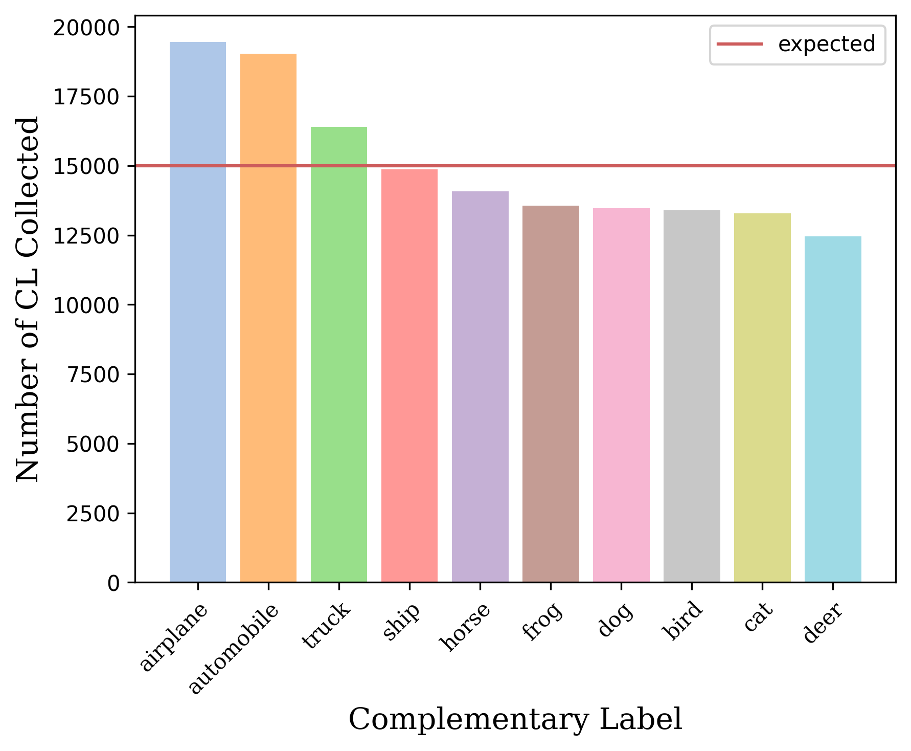
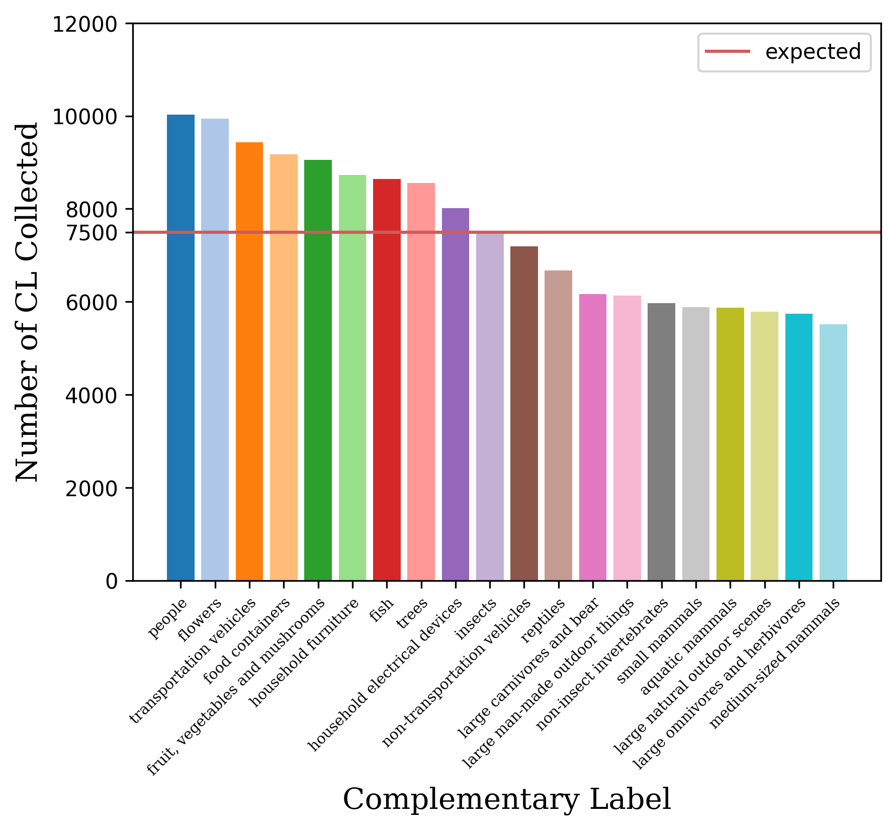
Next, we analyze the distribution of the collected complementary labels. The frequency of the complementary labels for the CLCIFAR datasets are reported in Figure 1. As we can see in the figure, the annotators have specific bias on certain labels. For instance, the annotators have a preference for “airplane” and “automobile” in CLCIFAR10 and a preference for “people” and “flower” in CLCIFAR20. In CLCIFAR10, the annotations are biased towards the labels with longer names whereas in CLCIFAR20, they are biased towards the labels with shorter, more concrete and understandable names.

(a) CLCIFAR10

(b) CLCIFAR20

Figure 2: The empirical transition matrices of CLCIFAR10 and CLCIFAR20. The label names of CLCIFAR20 are abbreviated as indexes to save space. The full label names are provided in Appendix D.

Observation 3: biased transition matrix

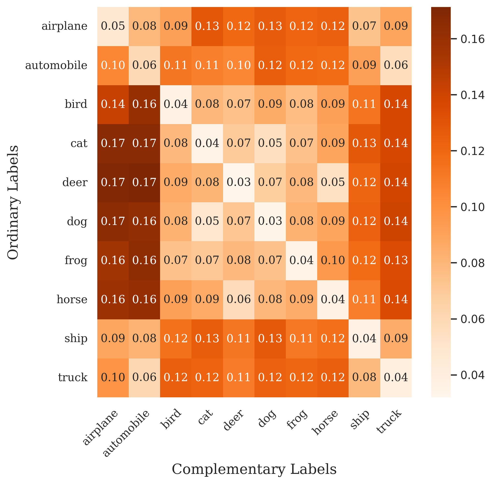
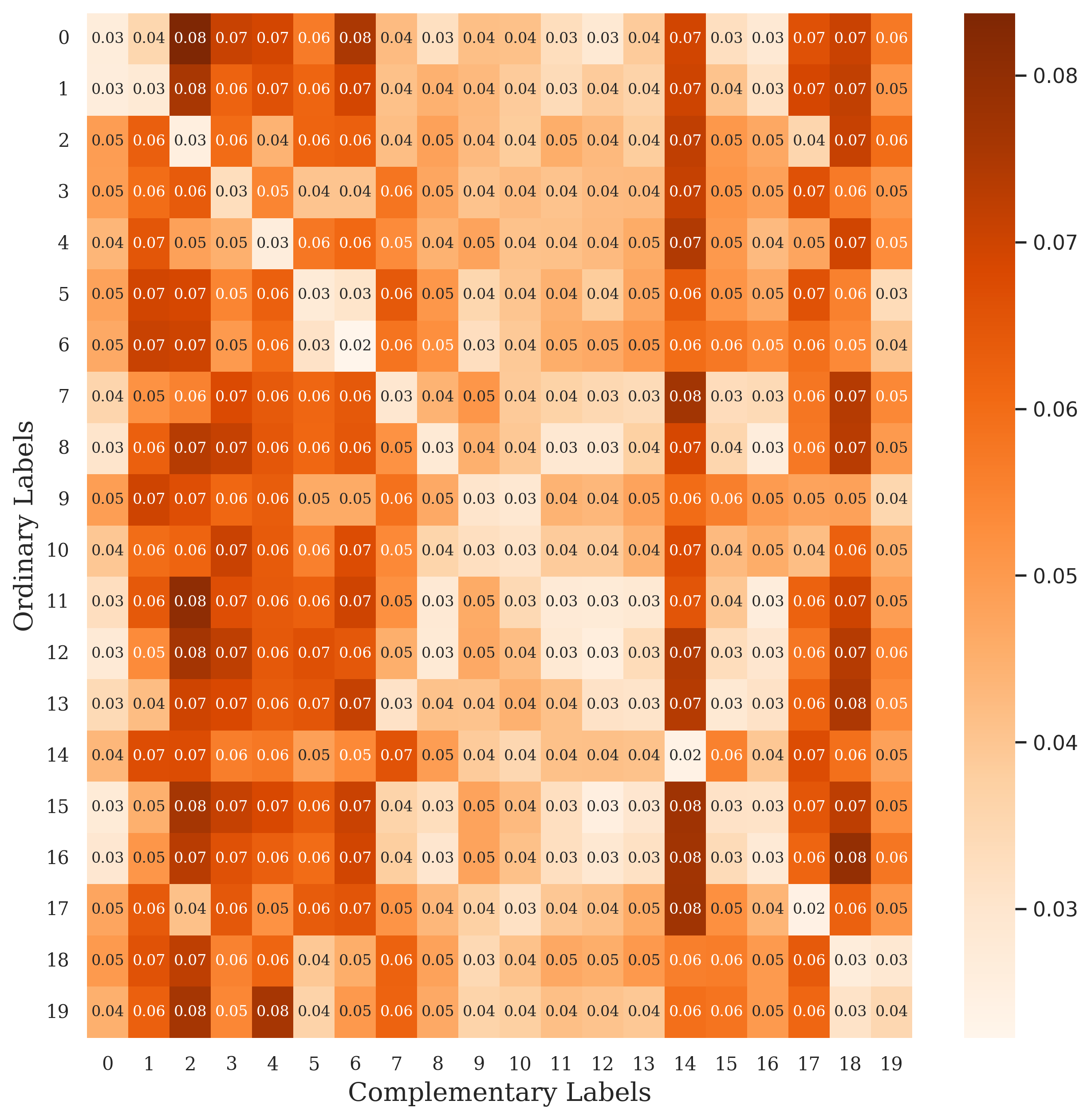
Finally, we visualize the empirical transition matrix using the collected complementary labels in Figure 2. Based on the first two observations, we could imagine that the transition matrix is biased. By inspecting Figure 2, we further discover that the bias in the complementary labels are dependent on the true labels. For instance, in CLCIFAR10, despite we see more annotations on airplane and automobile in aggregate, conditioning on the transportation-related labels (“airplane”, “automobile”, “ship” and “truck”), the distribution of the complementary labels becomes more biased towards other animal-related labels (“bird”, “cat”, etc.) Next, we study the impact of the bias and noise on existing CLL algorithms.

5 Experiments

In this section, we benchmarked several SOTA CLL algorithms on CLCIFAR10 and CLCIFAR20. A significant performance gap between the models trained on the humanly annotated CLCIFAR dataset and those trained on the synthetically generated complementary labels (CL) was observed in Section 5.1, which motivates us to analyze the possible reasons for the gap with the following experiments. To do so, we discuss the effect of three factors in the label generating process, feature dependency, noise, and biasedness, in Section 5.2, Section 5.3, and Section 5.4, respectively. From our experiment results, we conclude that noise is the dominant factor affecting the performance of the CLL algorithms on CLCIFAR. Another crucial component in applying CLL algorithms in practice is validation. We also discuss the empirical performance of the existing validation approaches in Section 5.5.

5.1 Standard benchmark on CLCIFAR10, CLCIFAR20

Baseline methods

Several SOTA CLL algorithms were selected for this benchmark. Some of them take the transition matrix $T$ as inputs, which we call $T$-informed methods, including

• Two versions of forward correction method [15]: FWD-U and FWD-T. They utilize a uniform transition matrix $T_{u}$ and an empirical transition matrix $T_{e}$ as input, respectively.

• Two versions of unbiased risk estimator with gradient ascent [8]: URE-GA-U with a uniform transition matrix $T_{u}$ and URE-GA-T with an empirical transition matrix $T_{e}$.

• Robust loss methods [9] for learning from noisy CL, including CCE, MAE, WMAE, GCE, and SL. We applied the gradient ascent technique [8] as recommended in the original paper.

In practice, the empirical transition matrix $T_{e}$ is not accessible to the learning algorithm, but we assume that the correct $T_{e}$ is given to FWD-T, URE-GA-T and the robust loss methods for simplicity.

We also included some algorithms that assume the transition matrix $T$ to be uniform, which we call $T$-agnostic methods, including

• Surrogate complementary loss [1] with the negative log loss (SCL-NL) and with the exponential loss (SCL-EXP),

• Discriminative modeling [6] (L-W) and its weighted variant (L-UW), and

• Pairwise-comparison (PC) with the sigmoid loss [7].

Implementation details

In this standard benchmark, for each data instance, we first randomly drew one CL from the the collected CLs to form a single CLL dataset. Then, we trained a ResNet-18 model using the baseline methods mentioned above on the single CLL dataset using the Adam optimizer for 300 epochs without learning rate scheduling. We left the benchmarks with multiple CLs in Appendix A.1. The weight decay was fixed at $10^{-4}$ and the batch size was set to 512. The experiments were run with NVIDIA V100 or RTX 2070. For better generalization, we applied standard data augmentation technique, RandomHorizontalFlip, RandomCrop, and normalization to each image. The learning rate was selected from $\{10^{-3}$, $5\times 10^{-4}$, $10^{-4}$, $5\times 10^{-5}$, $10^{-5}\}$ using a 10% hold-out validation set. We selected the learning rate with the best classification accuracy on the validation dataset. Note that here we assumed the ground-truth labels in the validation dataset are known. We will discuss other validation objectives that rely only on complementary labels in Section 5.5. As CLL algorithms are prone to overfitting [8, 1], some previous works did not use the model after training for evaluation. Instead, early-stopping was performed by evaluating the model on the validation dataset and selecting the epoch with the highest validation accuracy. For completeness, we considered both settings, and used “(ES)” to indicate that the aforementioned early-stopping technique is employed. For reference, we also performed the experiments on synthetically-generated CLL dataset, where the CLs were generated uniformly and noiselessly, denoted uniform-CIFAR.

Results and discussion

As we can observe in Table 1, there is a significant performance gap between the humanly annotated dataset, CLCIFAR, and the synthetically generated dataset, uniform-CIFAR. The difference between the two datasets can be divided into three parts: (a) whether the generation of complementary labels depends on the feature, (b) whether there is noise, and (c) whether the complementary labels are generated with bias. A negative answer to those questions simplify the problem of CLL. We can gradually simplify CLCIFAR to uniform-CIFAR by chaining those assumptions as follows :

$$\boxed{\text{CLCIFAR}}\;\xRightarrow[\text{Remove feature dependency}]{\text{Section~{}\ref{sec:exp-feat}}}\;\;\xRightarrow[\text{Remove noise}]{\text{Section~{}\ref{sec:exp-noise}}}\;\;\xRightarrow[\text{Remove biasedness}]{\text{Section~{}\ref{sec:exp-bias}}}\;\boxed{\text{uniform-CIFAR}}$$

In the following subsections, we will analyze how these three factors affect the performance of the CLL algorithms.

Table 1: Standard benchmark results on CLCIFAR and uniform-CIFAR datasets. Mean accuracy ($\pm$ standard deviation) on the testing dataset from four trials with different random seeds. Highest accuracy in each column is highlighted in bold.

	uniform-CIFAR10		CLCIFAR10		uniform-CIFAR20		CLCIFAR20
methods	valid_acc	valid_acc (ES)	valid_acc	valid_acc (ES)	valid_acc	valid_acc (ES)	valid_acc	valid_acc (ES)
FWD-U	69.17$\pm$1.22	69.79$\pm$1.01	34.09$\pm$1.16	36.83$\pm$1.17	20.24$\pm$0.52	20.62$\pm$0.49	7.47$\pm$0.37	8.27$\pm$0.77
FWD-R	-	-	28.88$\pm$0.65	38.9$\pm$1.57	-	-	16.14$\pm$1.11	20.31$\pm$0.25
URE-GA-U	54.62$\pm$0.6	54.94$\pm$1.34	34.59$\pm$0.76	36.39$\pm$0.67	15.41$\pm$0.97	16.59$\pm$0.61	7.59$\pm$0.36	10.06$\pm$0.72
URE-GA-R	-	-	28.7$\pm$1.39	30.94$\pm$1.66	-	-	5.24$\pm$0.2	5.46$\pm$0.28
SCL-NL	67.15$\pm$1.9	68.64$\pm$1.98	33.8$\pm$0.52	37.81$\pm$2.12	20.04$\pm$0.48	20.68$\pm$0.46	7.58$\pm$0.66	8.53$\pm$0.29
SCL-EXP	64.86$\pm$0.44	65.4$\pm$0.32	34.59$\pm$0.72	36.96$\pm$0.18	19.4$\pm$0.76	21.03$\pm$0.64	7.55$\pm$0.51	8.11$\pm$0.71
L-W	56.21$\pm$0.54	59.18$\pm$0.46	28.04$\pm$0.38	34.55$\pm$2.05	14.35$\pm$0.74	19.11$\pm$1.29	7.08$\pm$1.1	8.74$\pm$0.42
L-UW	60.88$\pm$0.77	62.43$\pm$0.46	30.63$\pm$1.87	35.13$\pm$1.56	16.01$\pm$0.89	19.42$\pm$0.42	7.36$\pm$0.33	8.71$\pm$0.31
PC-sigmoid	28.20$\pm$0.58	39.29$\pm$0.87	24.38$\pm$2.18	35.88$\pm$0.98	9.72$\pm$0.49	16.45$\pm$0.64	9.27$\pm$0.37	14.26$\pm$1.04
MAE	57.37$\pm$0.48	58.50$\pm$0.97	16.30$\pm$2.27	19.44$\pm$4.41	16.72$\pm$1.52	17.63$\pm$1.63	5.11$\pm$0.11	5.87$\pm$0.26

5.2 Feature dependency

In this experiment, we verified whether the performance gap resulted from the feature-dependent generation of practical CLs. Conceivably, even if two images belong to the same class, the distribution on the complementary labels could be different. On the other hand, the distributional difference could also be too small to affect model performance, e.g., if $P(\bar{Y}\mid Y,X)\approx P(\bar{Y}\mid Y)$ for most $X$. Consequently, we decided to further look into whether this assumption can explain the performance gap. To observe the effects of approximating $P(\bar{Y}\mid Y,X)$ with $P(\bar{Y}\mid Y)$, we generated two synthetic complementary datasets, CLCIFAR10-iid and CLCIFAR20-iid by i.i.d. sampling CLs from the empirical transition matrix in CLCIFAR10 and CLCIFAR20, respectively. We proceeded to benchmark the CLL algorithms on CLCIFAR-iid and presented the accuracy difference compared to CLCIFAR in Table 2.

Results and discussion

From Table 2, we observed that the accuracy barely changes on the resampled CLCIFAR-iid, suggesting that even if the complementary labels in CLCIFAR could be feature-dependent, this dependency does not affect the model performance significantly. Hence, there might be other factors contributing to the performance gap.

Table 2: Mean accuracy difference ($\pm$ standard deviation) of different CLL algorithms. A plus indicates the performance on is calculated as CLCIFAR-i.i.d. accuracy minus CLCIFAR accuracy.

	FWD-U	FWD-R	URE-GA-U	URE-GA-R	SCL-NL	SCL-EXP	L-W	L-UW	PC-sigmoid
CLCIFAR10-iid	-1.1$\pm$2.17	-0.36$\pm$1.15	-3.03$\pm$1.25	0.74$\pm$0.35	-0.67$\pm$1.81	-1.97$\pm$1.16	-2.5$\pm$0.56	-3.53$\pm$1.36	-2.03$\pm$2.05
CLCIFAR20-iid	-0.64$\pm$0.39	-3.53$\pm$1.13	-0.37$\pm$0.51	1.79$\pm$2.34	-0.28$\pm$0.61	-0.39$\pm$0.69	-0.5$\pm$1.37	-0.82$\pm$0.04	-2.24$\pm$0.52

5.3 Labeling noise

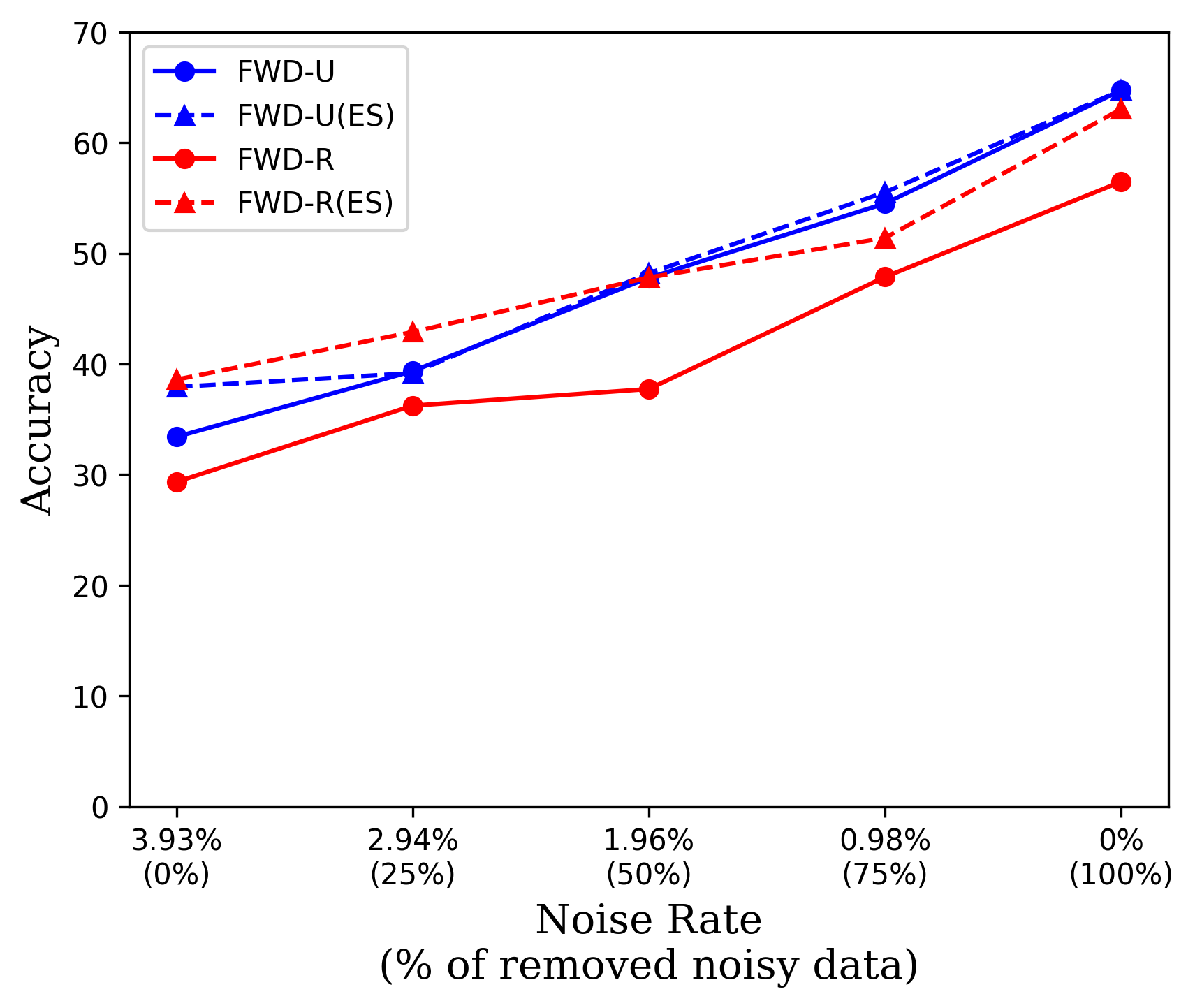
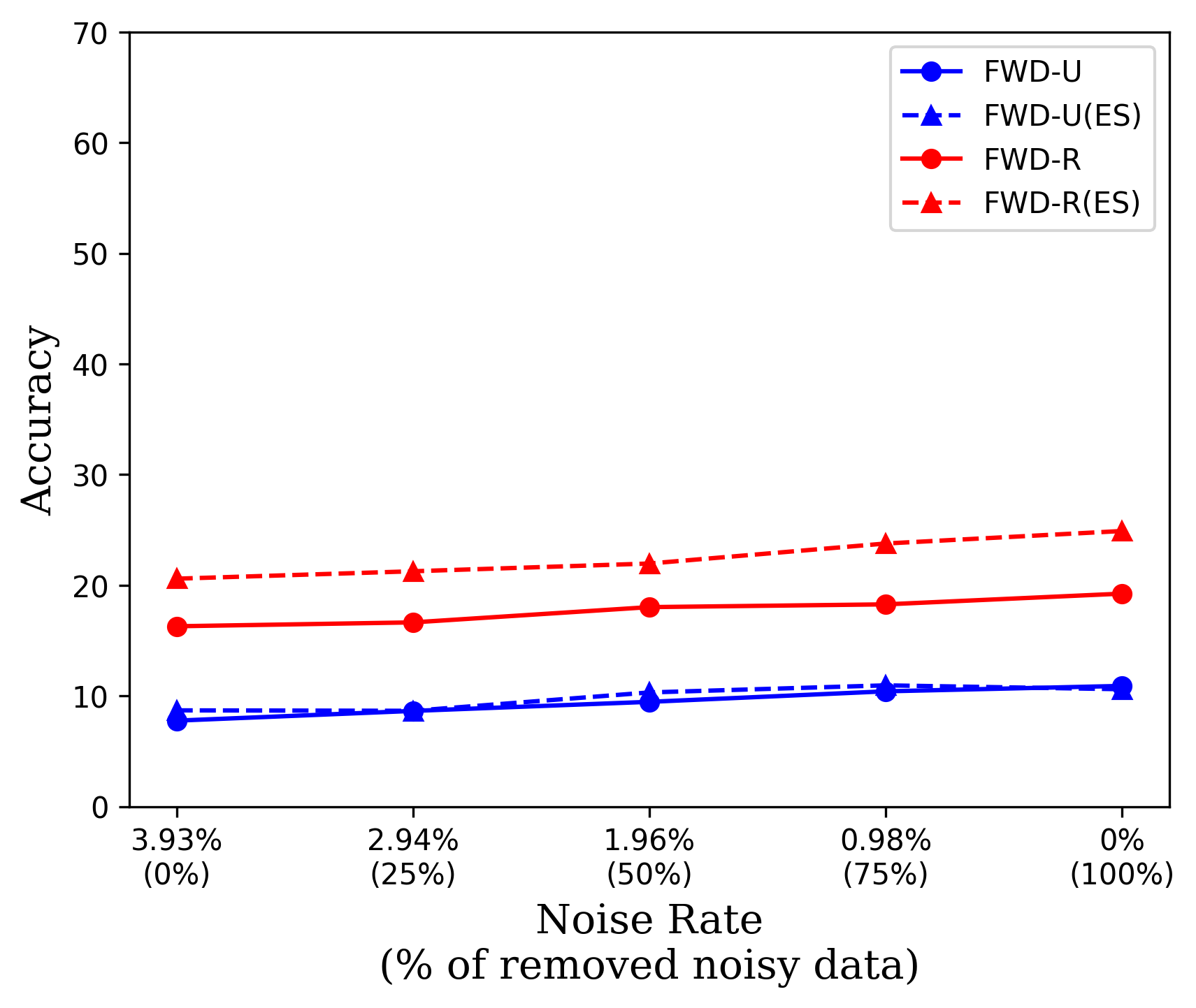
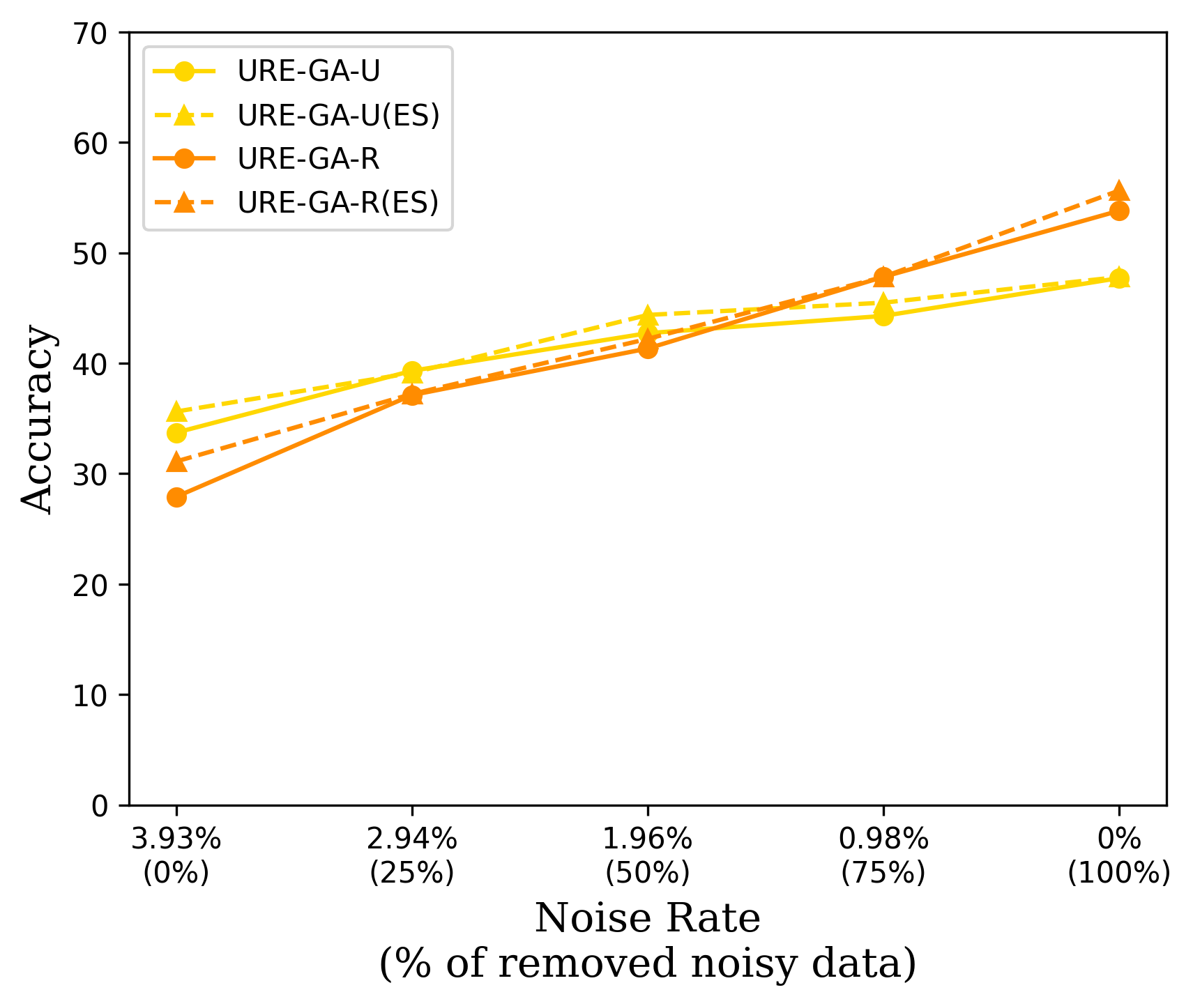
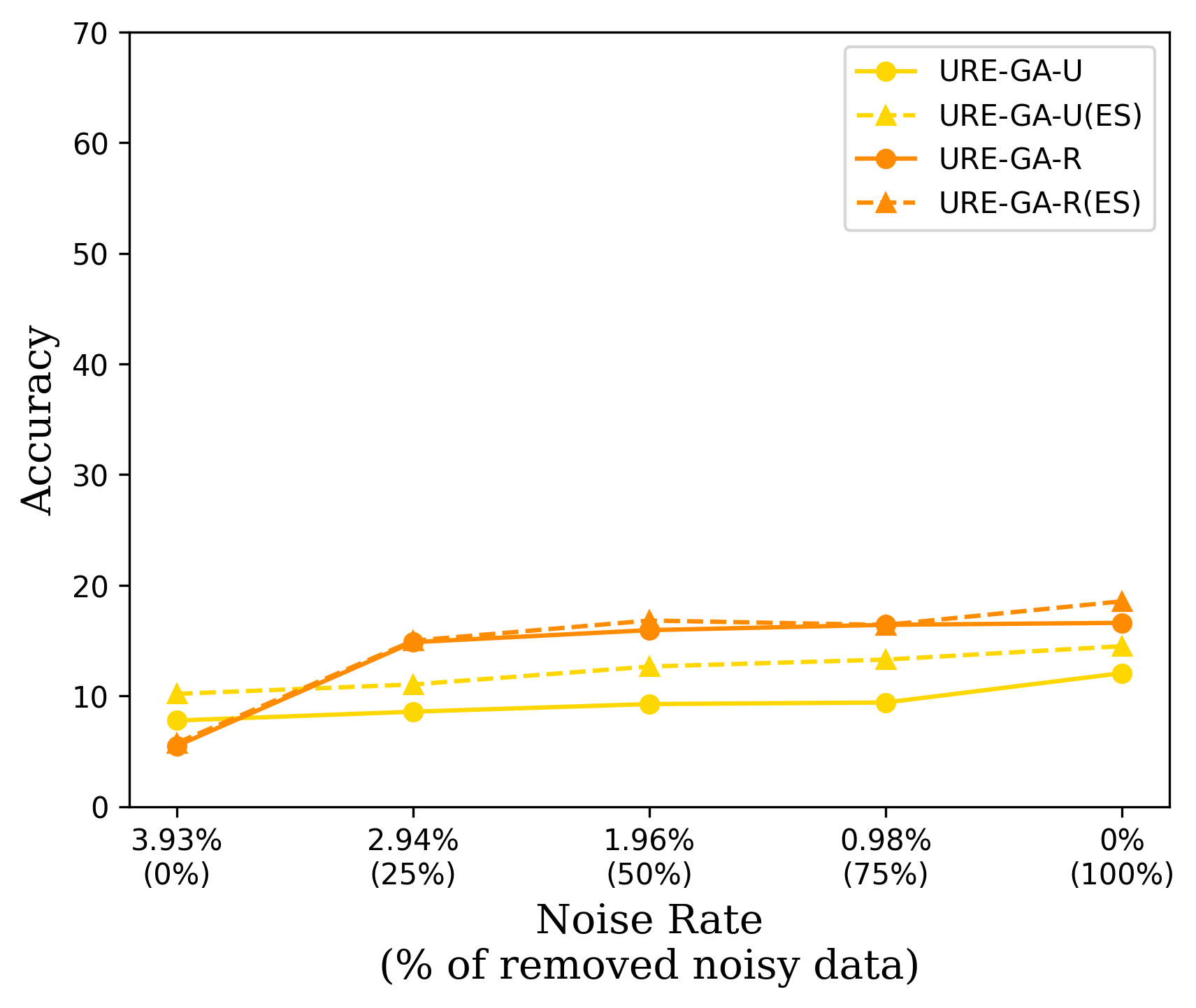
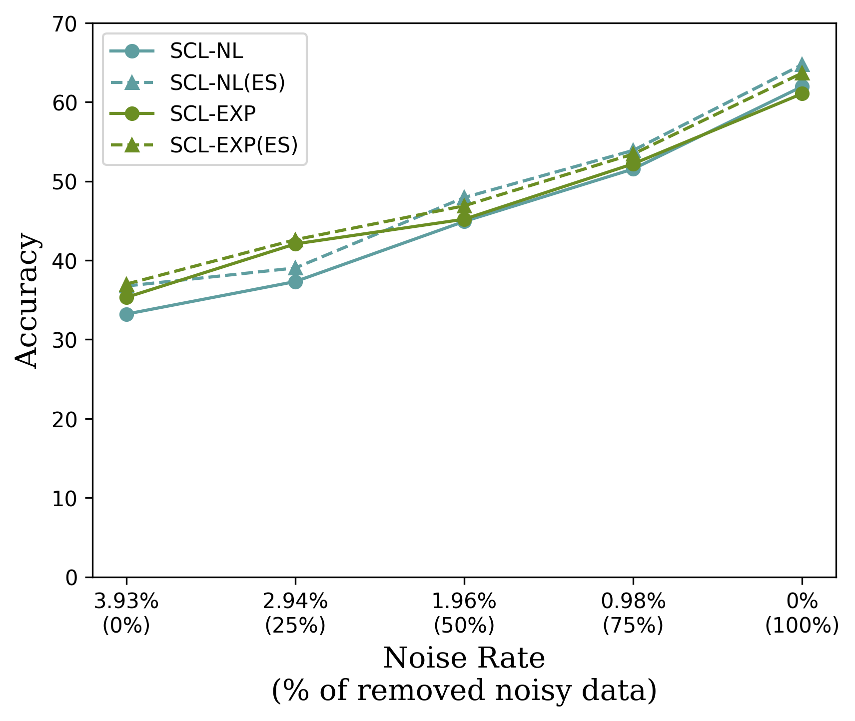
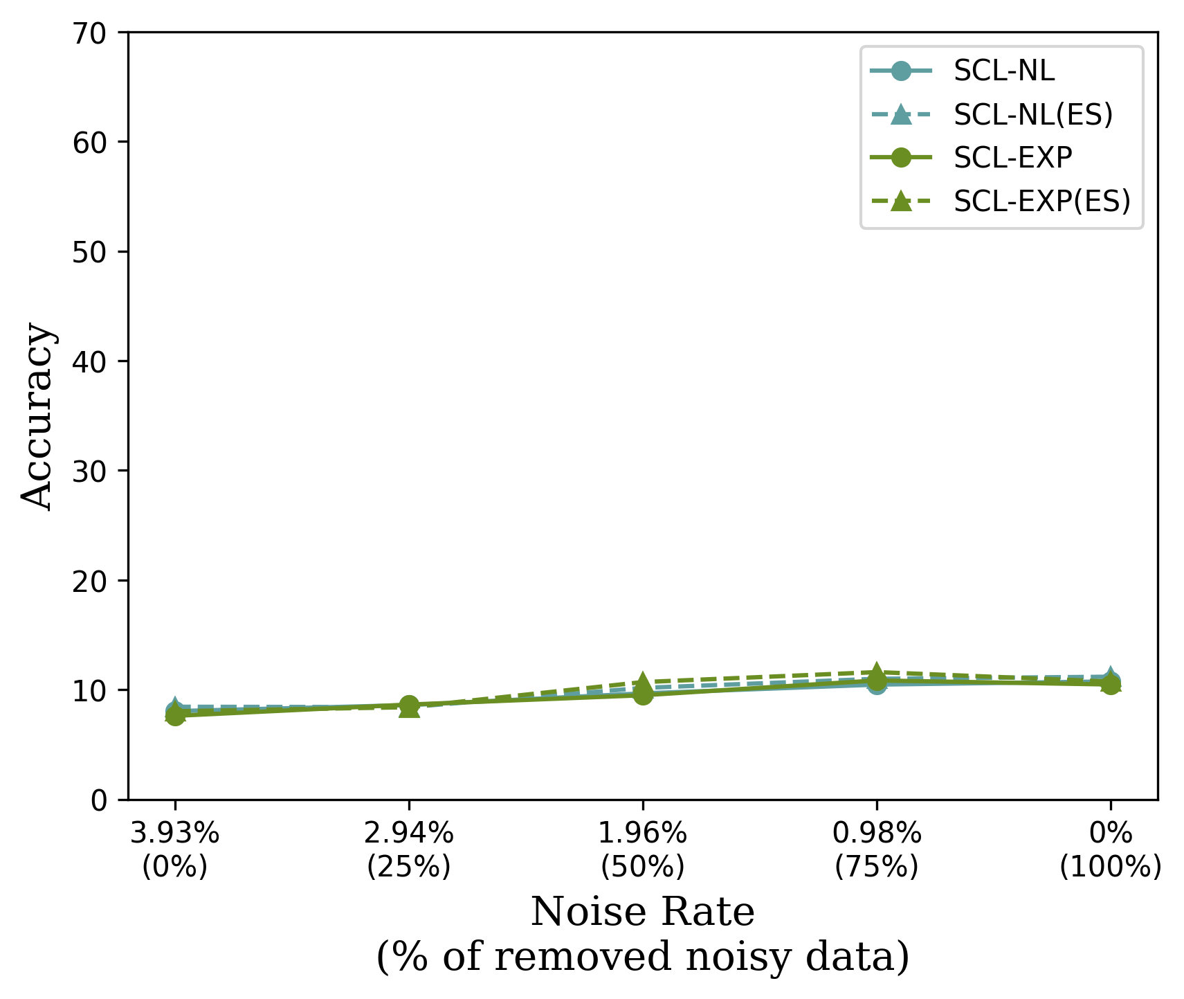
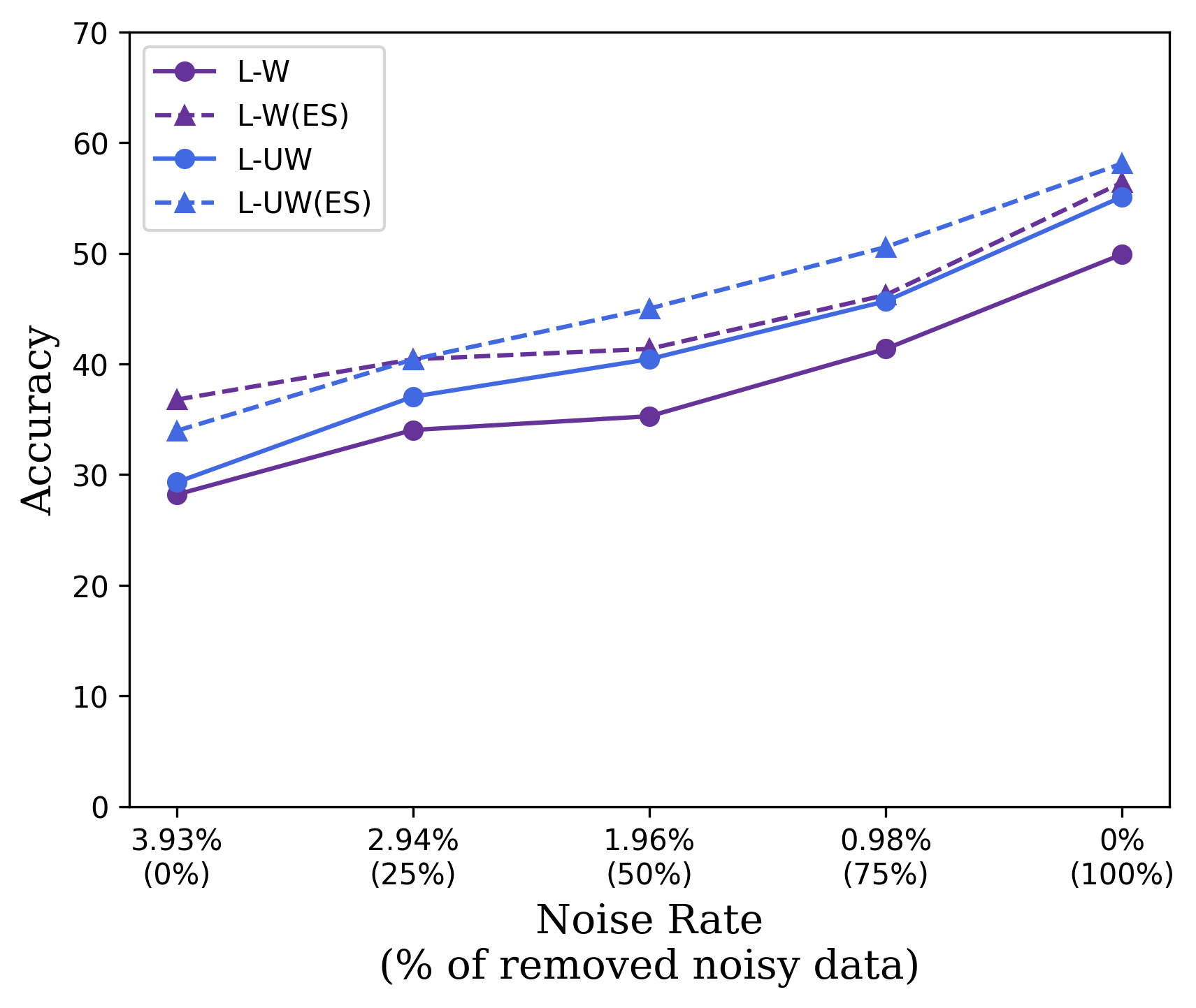
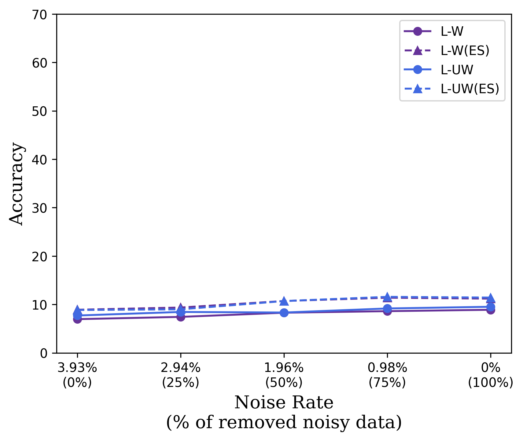
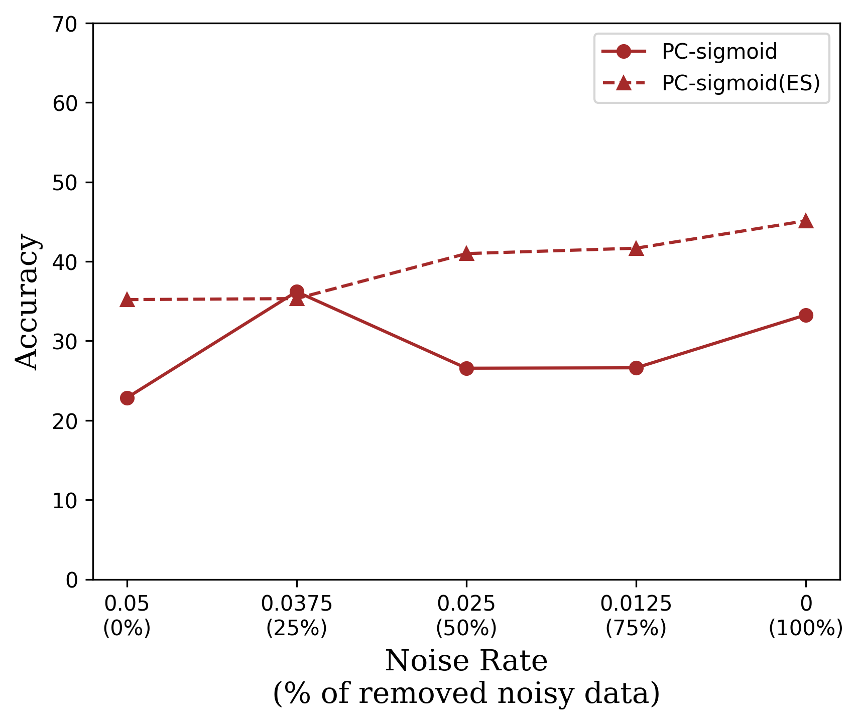
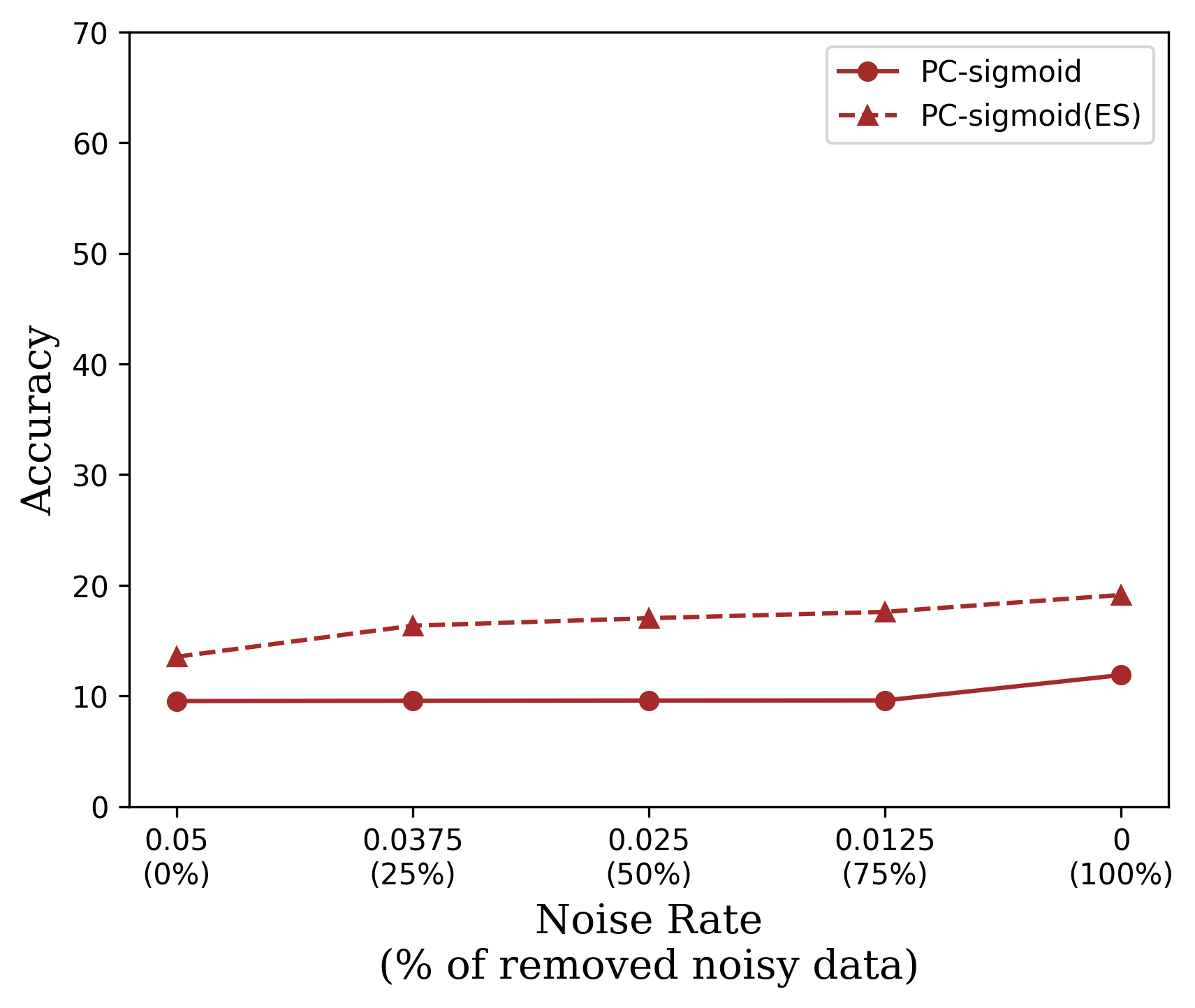
In this experiment, we further investigated the impact of the label noise on the performance gap. Specifically, we measured the accuracy on the noise-removed versions of CLCIFAR datasets, where varying percentages (0%, 25%, 50%, 75%, or 100%) of noisy labels are eliminated.

Results and discussion

We present the performance of FWD trained on thenoise-removed CLCIFAR10 dataset in the left figure in Figure 3. The results for other algorithms and the noise-removed CLCIFAR20 dataset can be found in Appendix C. From the figure, we observe a strong positive correlation between the performance and the proportion of removed noisy labels. When more noisy labels are removed, the performance gap diminishes and the accuracy approaches that of the ideal uniform-CLFAR dataset. Therefore, we conclude that the performance gap between the humanly annotated CLs and the synthetically generated CLs are primarily attributed to the label noise.

5.4 Biasedness of complementary labels

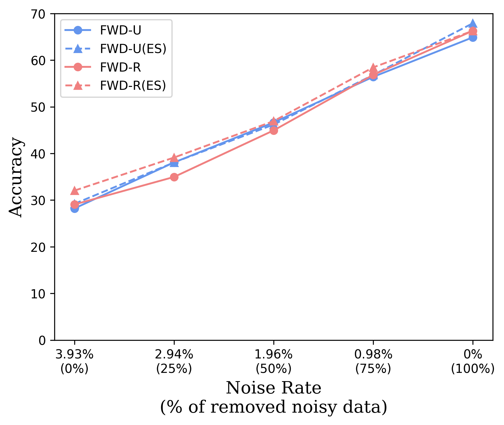
To further study the biasedness of CL as a potential factor contributing to the performance gap, we removed the biasedness from the noise-removed CLCIFAR dataset and examined the resulting accuracy. Specifically, we introduced the same level of uniform noise in uniform-CIFAR dataset and reevaluated the performance of FWD algorithms.

Results and discussion

The striking similarity between the two curves in the right figure in Figure 3 shows that the accuracy is significantly influenced by label noise, while the biasedness of CL has a negligible impact on the results. Furthermore, we observe that the accuracy difference between the results of the last epoch and the early-stopping results becomes smaller when the model is trained on the uniformly generated CLs. That is, the $T$-informed methods are more prone to overfitting when there is a bias in the CL generation.

With the experiment results in Section 5.2, 5.3, and 5.4, we can conclude that the performance gap between humanly annotated CL and synthetically generated CL is primarily attributed to label noise. Additionally, the biasedness of CLs may potentially contribute to overfitting, while the feature-dependent CLs do not detrimentally affect performance empirically. It is worth noting that in the last row of Table 1, the MAE methods that can learn from noisy CL fails to generalize well in the practical dataset. These results suggest that more research on learning with noisy complementary labels can potentially make CLL more realistic.

Figure 3: Accuracy of FWD-U and FWD-R on the noise-removed CLCIFAR10 dataset (Left) and the uniform-CIFAR10 dataset with uniform noise (Right) at varying noise rates.

5.5 Validation objectives

Validating the model performance solely with CL poses a non-trivial challenge. To offer an empirical analysis from the perspective of practical datasets, we evaluated the models using a purely complementary validation set and employed two validation objectives, including unbiased risk estimator (URE) [8] and surrogate complementary estimation loss (SCEL) [10]. We used these two validation objectives to select the optimal learning rate from $\{10^{-3}$, $5\times 10^{-4}$, $10^{-4}$, $5\times 10^{-5}$, $10^{-5}\}$ and provides the accuracy on testing set in Table 3. For completeness, we also provide the accuracy of models selected using a validation set that contains an equal number of true labels.

Results and discussion

Based on our results, we do not observe a deterministic trend in the accuracy between the models selected by URE or SCEL. To further visualize the difference between a pure complementary validation set and a ordinary validation set, we calculated the accuracy difference between the model selected using the ordinary validation set and the best models selected from either URE or SCEL. The results were reported in the gap column in Table 3. For some algorithms and datasets, a non-negligible gap was observed. Whether this gap could be further reduced remains open. Deeper understanding on the validation of CLL can potentially help making CLL more practical.

Table 3: The testing accuracy of models evaluated with URE and SCEL.

	uniform-cifar10				clcifar10				uniform-cifar20				clcifar20
	URE	SCEL	valid acc	gap ($\downarrow$)	URE	SCEL	valid acc	gap ($\downarrow$)	URE	SCEL	valid acc	gap ($\downarrow$)	URE	SCEL	valid acc	gap ($\downarrow$)
FWD-U	22.36	45.63	48.44	2.81	32.54	33.02	34.09	1.07	16.02	16.02	17.4	1.38	7.33	7.33	7.47	0.14
FWD-R	-	-	-	-	28.88	19.13	28.88	0	-	-	-	-	10.74	9.8	16.14	5.4
URE-GA-U	39.24	39.24	39.55	0.31	31.34	34.59	34.59	0	13.12	12.64	13.52	0.4	7.28	7.85	7.59	-0.26
URE-GA-R	-	-	-	-	26.61	28.18	28.7	0.52	-	-	-	-	5.2	5.36	5.24	-0.12
SCL-NL	22.83	36.44	48.2	11.76	32.49	33.32	33.8	0.48	14.16	16.55	16.55	0	7.12	6.5	7.58	0.46
SCL-EXP	22.72	22.72	46.79	24.07	33.15	31.26	34.59	1.44	14.23	14.16	16.18	1.95	6.85	6.53	7.55	0.7
L-W	10.38	11.03	27.02	15.99	20.71	20.71	28.04	7.33	7.37	9.66	10.39	0.73	5.77	6.03	7.08	1.05
L-UW	9.93	9.93	31.3	21.37	22.97	22.97	30.63	7.66	7.68	7.68	12.33	4.65	5.9	5.9	7.36	1.46
PC-sigmoid	16.07	15.62	18.97	2.9	14.98	15.43	24.38	8.95	7.38	7.38	7.67	0.29	7.04	8.63	9.27	0.64

6 Conclusion

In this paper, we devised a protocol to collect complementary labels from human annotators. Utilizing this protocol, we curated two real-world datasets, CLCIFAR10 and CLCIFAR20, and made them publicly available to the research community. Through our meticulous analysis of these datasets, we confirmed the presence of noise and bias in the human-annotated complementary labels, challenging some of the underlying assumptions of existing CLL algorithms. Extensive benchmarking experiments revealed that noise is a critical factor that undermines the effectiveness of most existing CLL algorithms. Furthermore, the biased complementary labels can trigger overfitting, even for algorithms explicitly designed to leverage this bias information. These findings emphasize the need for the community to dedicate more effort to developing CLL algorithms that are robust to both noise and bias. The curated datasets pave the way for the community to create more practical and applicable CLL solutions.

Appendix

Appendix A More discussion on practical noise

Our work found out that the labeling noise is the main factor contributing to the performance gap between synthetic CL and practical CL. Hence, we conducted deeper investigation into some directions to handle the practical noise. In Section A.1, we discussed the performance improvement when more human-annotated complementary labels were available. In Section A.2, we designed the synthetic CLCIFAR-N dataset to study the difference between synthetic uniform noise and practical noise. In Section A.3, we provided the benchmark results of all robust loss methods to emphasize the essence of studying a practical complementary label dataset.

A.1 Multiple complementary labels

In this experiment, we studied the case when there were multiple CLs for a data instance. We duplicated the data instance and assigned them with another practical label from the annotators. The results of this experiment were summarized in Table 4.

For CLCIFAR10, we observe that the model achieved better learning performance when trained on data instances with more CLs. However, the issue of overfitting persists even with the increased number of labels. In the case of CLCIFAR20, we found that without employing early stopping techniques, it is challenging to achieve improved results as the number of labels increased. Furthermore, the overfitting problem becomes more pronounced with the increased number of labels. Overall, these findings shed light on the challenges posed by multiple CLs and the persistence of overfitting.

Table 4: Learning with Multiple CL: The figure shows the classification accuracy of each task with early stopping indicated in brackets. The highest accuracy in each column is bolded for ease of comparison.

	CLCIFAR10			CLCIFAR20
num CL	1	2	3	1	2	3
FWD-U	34.09(36.83)	41.95(41.53)	42.88(45.18)	7.47(8.27)	8.28(8.78)	8.15(10.27)
FWD-R	28.88(38.9)	34.33(47.07)	37.84(49.76)	16.14(20.31)	16.99(23.41)	15.54(24.19)
URE-GA-U	34.59(36.39)	45.71(44.85)	45.97(47.97)	7.59(10.06)	8.42(11.52)	8.53(12.75)
URE-GA-R	28.7(30.94)	42.73(43.34)	44.73(47.36)	5.24(5.46)	6.77(6.92)	5.0(5.55)
SCL-NL	33.8(37.81)	40.67(42.58)	43.39(45.2)	7.58(8.53)	6.77(6.92)	5.0(5.55)
SCL-EXP	34.59(36.96)	40.89(42.99)	44.4(47.9)	7.55(8.11)	7.42(8.39)	8.0(9.31)
L-W	28.04(34.55)	34.96(41.83)	39.05(47.46)	7.08(8.74)	8.06(8.76)	8.03(10.18)
L-UW	30.63(35.13)	38.05(43.32)	39.49(45.82)	7.36(8.71)	7.03(8.55)	7.86(10.11)
PC-sigmoid	24.38(35.88)	25.63(39.82)	33.89(43.75)	9.27(14.26)	11.91(16.07)	17.68(14.13)

A.2 Benchmarks with synthetic noise

Generation process of CLCIFAR-N

Inspired by the conclusions drawn in Section 5.3, we investigated another avenue of research: the generalization capabilities of methods when transitioning from synthetic datasets with uniform noise to practical datasets. To obtain a general synthetic dataset with minimum assumption, we introduced CLCIFAR-N. This synthetic dataset contains unifrom CL and uniform real world noise from CLCIFAR dataset. The complementary labels of CLCIFAR-N are i.i.d. sampled from $T_{syn}$, where the diagonal entries are set to be $3.93\%/10$ (for generating CL for CIFAR10) or $2.8\%/20$ (for generating CL for CIFAR20). The non-diagonal entries are uniformly distributed. This construction allows us to generate a synthetic dataset that mimics real-world scenarios more closely with minimum knowledge.

Benchmark results

We ran the benchmark experiments with the identical settings as in Section 5.1 and present the results in Table 5. The performance difference between sythetic noise and practical noise are illustrated in the diff columns. A smaller difference indicates a better generalization capability of the models. Interestingly, the robust loss methods exhibit superiority on the synthetic CLCIFAR10-N dataset but struggle to generalize well on real-world datasets. This finding suggests the existence of fundamental differences between synthetic noise and practical noise. Further investigation into these differences is left as an avenue for future research.

Table 5: Benchmark results on CLCIFAR-N datasets. The classification accuracy difference is calculated by subtracting the practical CLCIFAR dataset from the performance on the synthetic CLCIFAR-N dataset.

	CLCIFAR10-N	diff($\downarrow$)	CLCIFAR20-N	diff($\downarrow$)
FWD-U	37.1	2.2	7.58	0.11
FWD-R	-	-	-	-
URE-GA-U	31.29	-3.3	8.1	0.5
URE-GA-R	-	-	-	-
SCL-NL	37.79	2.06	7.75	0.16
SCL-EXP	35.86	3.19	6.95	-0.59
L-W	30.1	2.06	6.16	-0.91
L-UW	32.69	2.05	6.89	-0.47
PC-sigmoid	19.64	-4.73	6.54	-2.72
CCE	32.34	13.45	5.71	0.71
MAE	41.34	23.09	6.83	1.83
WMAE	37.62	22.26	6.36	1.08
GCE	35.00	18.71	6.7	1.7
SL	29.98	12.29	6.08	1.05

A.3 Results of the robust loss methods

The original design of the robust loss aims to obtain the optimal risk minimizer even in the presence of corrupted labels. However, their methods do not generalized well on practical datasets. The results are provided in Table 6. In other words, solely considering synthetic noisy CLs does not guarantee performance on real-world datasets. These results once again underscore the importance of the CLCIFAR dataset.

Table 6: Standard benchmark results on CLCIFAR and uniform-CIFAR datasets for the robust loss method. Mean accuracy ($\pm$ standard deviation) on the testing dataset from four trials with different random seeds. Highest accuracy in each column is highlighted in bold.

	uniform-CIFAR10		CLCIFAR10		uniform-CIFAR20		CLCIFAR20
methods	valid_acc	valid_acc (ES)	valid_acc	valid_acc (ES)	valid_acc	valid_acc (ES)	valid_acc	valid_acc (ES)
CCE	46.57$\pm$1.75	49.51$\pm$0.73	16.18$\pm$2.97	20.18$\pm$3.39	12.54$\pm$0.40	14.62$\pm$1.29	5.07$\pm$0.05	5.41$\pm$0.30
MAE	57.37$\pm$0.48	58.50$\pm$0.97	16.30$\pm$2.27	19.44$\pm$4.41	16.72$\pm$1.52	17.63$\pm$1.63	5.11$\pm$0.11	5.87$\pm$0.26
WMAE	-	-	13.01$\pm$1.89	15.51$\pm$0.75	-	-	5.31$\pm$0.27	6.65$\pm$0.65
GCE	58.10$\pm$1.54	59.44$\pm$2.30	14.31$\pm$1.44	18.97$\pm$2.16	15.86$\pm$1.93	17.09$\pm$1.19	5.21$\pm$0.29	5.76$\pm$0.32
SL	41.13$\pm$1.64	42.64$\pm$0.11	16.45$\pm$2.80	19.28$\pm$3.16	13.60$\pm$0.55	15.70$\pm$1.23	5.44$\pm$0.29	6.59$\pm$0.43

Appendix B More discussion on biasedness

In addition to the label noise, the biasedness of CL in practical dataset would lead to overfitting, especially for those T-informed algorithms. We conducted deeper investigation into this phenomenon. In Section B.1, we demonstrated the necessity of employing data augmentation techniques to prevent overfitting. In Section B.2, we attempted to address the issue of overfitting by employing an interpolated transition matrix for regularization.

B.1 Ablation on data augmentation

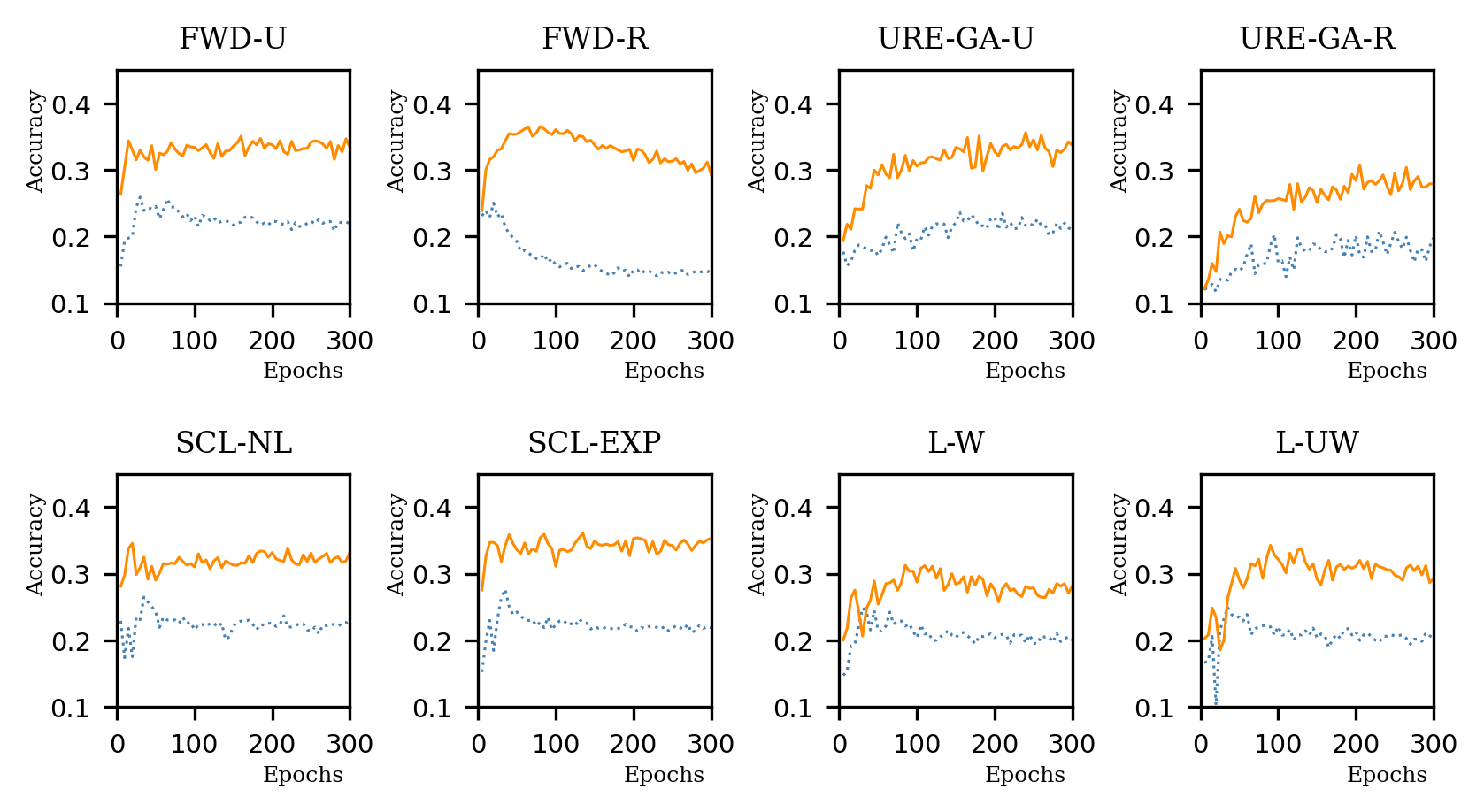
To further investigate the significance of data augmentation, we conducted identical experiments without employing data augmentation during the training phase. As we can observe in the training curves in Figure 4, data augmentation could improve the testing accuracy of all the algorithms we considered.

We also provide the results without the use of data augmentation techniques in Table 7, and we observed that almost all methods suffered from overfitting. It is worth noting that URE with gradient ascent suffers less compared to the other methods. The reason might be that reversing the gradient of the class with negative loss (the overfitting class) can be seen as a regularization technique. Therefore, URE with GA methods can be more resistant to overfitting in practical datasets.

Figure 4: The Overfitting accuracy curve of FWD, URE, SCL-NL, L-W. The dotted line represents the accuracy obtained without data augmentation, while the solid line represents the accuracy with data augmentation included for reference. The accuracy of FWD, SCL-NL, SCL-EXP, L-W, L-UW methods reaches its highest at approximately the 50 epoches and converges to some lower point. The detail numbers are in appendix 7

Table 7: The overfitting results when there is no data augmentation.

	uniform-CIFAR10		CLCIFAR10		uniform-CIFAR20		CLCIFAR20
methods	valid_acc	valid_acc (ES)	valid_acc	valid_acc (ES)	valid_acc	valid_acc (ES)	valid_acc	valid_acc (ES)
FWD-U	48.44	49.33	21.29	25.59	17.4	17.97	6.91	7.32
FWD-R	-	-	14.97	28.3	-	-	6.82	14.67
URE-GA-U	39.55	39.67	21.0	23.53	13.52	14.08	5.55	8.38
URE-GA-R	-	-	19.81	20.8	-	-	5.0	6.43
SCL-NL	48.2	48.27	21.96	26.51	16.55	17.54	7.1	7.92
SCL-EXP	46.79	47.52	21.89	27.66	16.18	17.89	6.9	7.3
L-W	27.02	44.78	20.06	27.6	10.39	16.3	5.64	8.02
L-UW	31.3	46.38	20.28	26.26	12.33	16.32	6.03	8.14
PC-sigmoid	18.97	33.26	-	-	7.67	10.41	-	-

B.2 Ablation on interpolation between $T_{u}$ and $T_{e}$

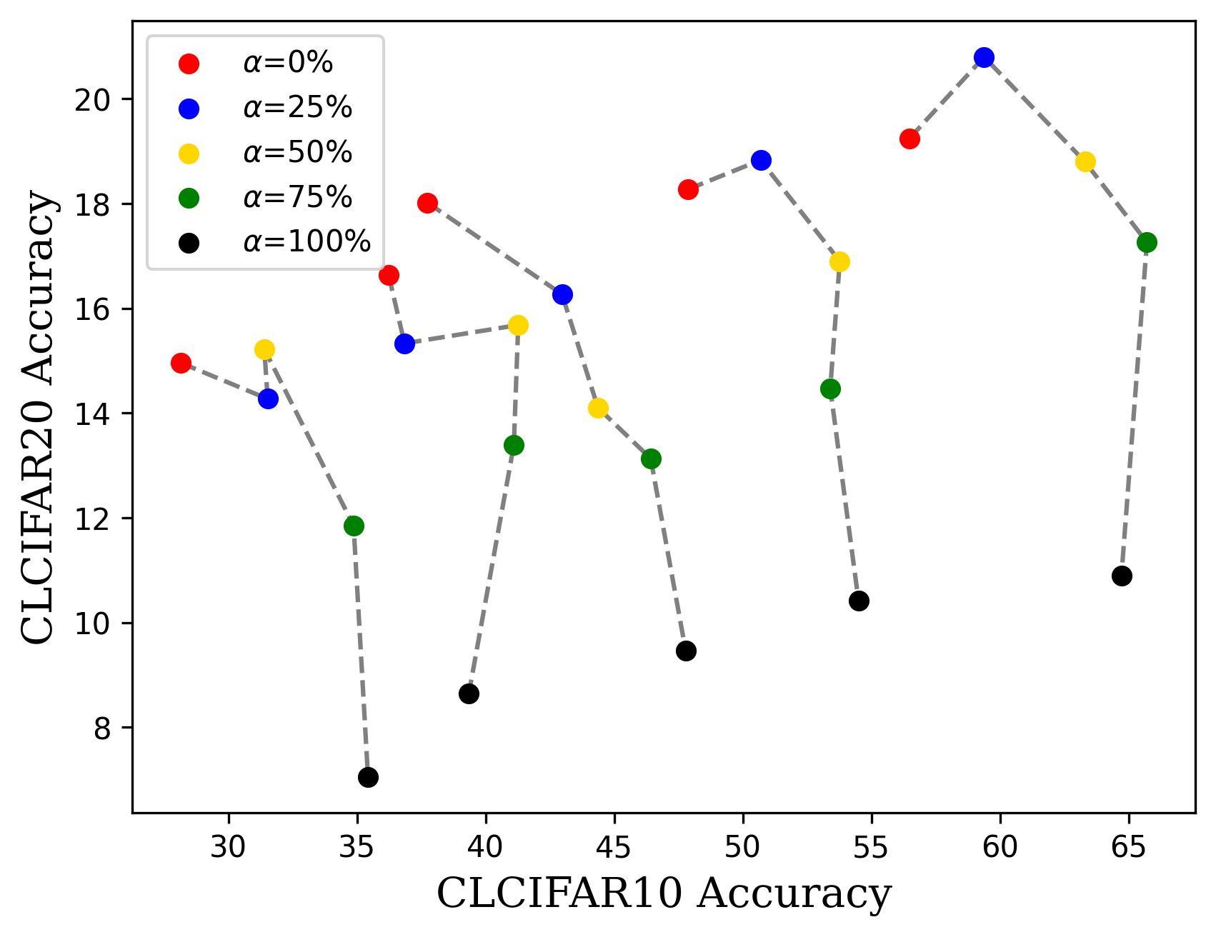
In Table 1, we discovered that the $T$-informed methods did not always deliver better testing accuracy when $T_{e}$ is given. Looking at the difference between the accuracy of using early-stopping and not using early-stopping, we observe that when the $T_{u}$ is given to the $T$-informed methods, the difference becomes smaller. This suggests that $T$-informed methods using the empirical transition matrix has greater tendency to overfitting. On the other hand, $T$-informed methods using the uniform transition matrix could be a more robust choice.

We observe that the uniform transition matrix $T_{u}$ acts like a regularization choice when the algorithms overfit on CLCIFAR. This results motivate us to study whether we can interpolate between $T_{u}$ and $T_{e}$ to let the algorithms utilize the information of transition matrix while preventing overfitting. To do so, we provide an interpolated transition matrix $T_{\text{int}}=\alpha T_{u}+(1-\alpha)T_{e}$ to the algorithm, where $\alpha$ controls the scale of the interpolation. As FWD is the $T$-informed method with the most sever overfitting when using $T_{u}$, we performed this experiment using FWD adn reported the results in Figure 5. As shown in Figure 5, FWD can learn better from an interpolated $T_{\text{int}}$, confirming the conjecture that $T_{u}$ can serve as a regularization role.

Figure 5: The last epoch accuracy of CLCIFAR10 and CLCIFAR20 for FWD algorithm with an $\alpha$-interpolated transition matrix $T_{\text{int}}$. The five solid points on each cruve represent different noise cleaning rate: 0%, 25%, 50%, 75%, 100% from left to right.

Appendix C Additional charts for CLCIFAR dataset with data cleaning

We remove 0%, 25%, 50%, 75%, 100% of the noisy data in CLCIFAR10 and CLCIFAR20 datasets. We discover that by removing the noisy data in the practical dataset, the practical performance gaps vanish for all the CLL algorithms. Therefore, we can conclude that the main obstacle to the practicality of CLL is label noise.

(a) FWD-(U/R) on CLCIFAR10

(b) FWD-(U/R) on CLCIFAR20

(a) URE-GA-(U/R) on CLCIFAR10

(b) URE-GA-(U/R) on CLCIFAR20

(a) SCL-(NL/EXP) on CLCIFAR10

(b) SCL-(NL/EXP) on CLCIFAR20

(a) L-(W/UW) on CLCIFAR10

(b) L-(W/UW) on CLCIFAR20

(a) PC-sigmoid on CLCIFAR10

(b) PC-sigmoid on CLCIFAR20

Appendix D Label names of CLCIFAR20

Index	Full Label Name
0	aquatic mammals
1	fish
2	flowers
3	food containers
4	fruit, vegetables and mushrooms
5	household electrical devices
6	household furniture
7	insects
8	large carnivores and bear
9	large man-made outdoor things
10	large natural outdoor scenes
11	large omnivores and herbivores
12	medium-sized mammals
13	non-insect invertebrates
14	people
15	reptiles
16	small mammals
17	trees
18	transportation vehicles
19	non-transportation vehicles

Appendix E Broader impacts

The datasets may advance the alorithms for learning from complementary labels. Those algorithms could learn a classifier with weak information. The privacy of the users may be easier to compromised as a result. We suggest the practitioners pay attention to the privacy issues when trying to utilize the collected datasets and the CLL algorithms.

Appendix F Access to the dataset and codes for reproduce

Please refer to the following link: https://github.com/ntucllab/complementary_cifar

References

- Chou et al. [2020] Y.-T. Chou, G. Niu, H.-T. Lin, and M. Sugiyama. Unbiased risk estimators can mislead: A case study of learning with complementary labels, 2020.
- Cour et al. [2011] T. Cour, B. Sapp, and B. Taskar. Learning from partial labels. The Journal of Machine Learning Research, 12:1501–1536, 2011.
- Denis [1998] F. Denis. Pac learning from positive statistical queries. In Algorithmic Learning Theory: 9th International Conference, ALT’98 Otzenhausen, Germany, October 8–10, 1998 Proceedings 9, pages 112–126. Springer, 1998.
- Feng et al. [2020] L. Feng, T. Kaneko, B. Han, G. Niu, B. An, and M. Sugiyama. Learning with multiple complementary labels. In International Conference on Machine Learning, pages 3072–3081. PMLR, 2020.
- Frénay and Verleysen [2013] B. Frénay and M. Verleysen. Classification in the presence of label noise: a survey. IEEE transactions on neural networks and learning systems, 25(5):845–869, 2013.
- Gao and Zhang [2021] Y. Gao and M.-L. Zhang. Discriminative complementary-label learning with weighted loss. In International Conference on Machine Learning, pages 3587–3597. PMLR, 2021.
- Ishida et al. [2017] T. Ishida, G. Niu, W. Hu, and M. Sugiyama. Learning from complementary labels. Advances in neural information processing systems, 30, 2017.
- Ishida et al. [2019] T. Ishida, G. Niu, A. K. Menon, and M. Sugiyama. Complementary-label learning for arbitrary losses and models, 2019.
- Ishiguro et al. [2022] H. Ishiguro, T. Ishida, and M. Sugiyama. Learning from noisy complementary labels with robust loss functions. IEICE TRANSACTIONS on Information and Systems, 105(2):364–376, 2022.
- Lin and Lin [2023] W.-I. Lin and H.-T. Lin. Reduction from complementary-label learning to probability estimates. In Proceedings of the Pacific-Asia Conference on Knowledge Discovery and Data Mining (PAKDD), May 2023.
- Liu et al. [2023] S. Liu, Y. Cao, Q. Zhang, L. Feng, and B. An. Consistent complementary-label learning via order-preserving losses. In International Conference on Artificial Intelligence and Statistics, pages 8734–8748. PMLR, 2023.
- Sugiyama et al. [2022] M. Sugiyama, H. Bao, T. Ishida, N. Lu, T. Sakai, and G. Niu. Machine learning from weak supervision: An empirical risk minimization approach. MIT Press, 2022.
- Wang et al. [2021] D.-B. Wang, L. Feng, and M.-L. Zhang. Learning from complementary labels via partial-output consistency regularization. In IJCAI, pages 3075–3081, 2021.
- Wei et al. [2022] J. Wei, Z. Zhu, H. Cheng, T. Liu, G. Niu, and Y. Liu. Learning with noisy labels revisited: A study using real-world human annotations, 2022.
- Yu et al. [2018] X. Yu, T. Liu, M. Gong, and D. Tao. Learning with biased complementary labels, 2018.
- Zhou [2018] Z.-H. Zhou. A brief introduction to weakly supervised learning. National science review, 5(1):44–53, 2018.