Superfat points and associated tensor.

Abstract

We study the 0-dimensional schemes supported at one point in $n$-space which are $m$-symmetric, i.e. they intersect any curves passing through the point with length $m$. We characterize the maximal ones geometrically and we show that the maximal length for such a scheme is $m^{n}$ ($m$-superfat points) and we study properties of such schemes, in particular for $n=2$. We also study varieties defined by such schemes on Veronese and Segre-Veronese varieties.

Contents

1. Introduction.

2. Symmetric and superfat points in $\mathbb{P}^{n}$.

3. Superfat and $m$-symmetric points in $\mathbb{P}^{2}$.

4. 2-squares on Veronese surfaces.

4.1 The cuckoo varieties $QQ(V_{d,d})$.

5. 2-squares on Segre-Veronese surfaces.

5.1 2-squares in $\mathbb{P}^{1}\times\mathbb{P}^{1}$ and the Segre-Veronese $V_{2,2}$.

5.2 General, symmetric and partially symmetric $2^{4}$-tensors

5.3 The veriety $q_{2}(V_{2,2})$.

5.3 The varieties $V_{d,d}$ and their $q_{2}(V_{d,d})$, $d\geq 3$.

5.4 The cuckoo varieties $qq_{2}(V_{d,d})$.

1 Introduction

The ideas for this work sprang from problems we encountered in a previous one ([CGI]), related to the Jacobian (or Tjurina) scheme associated to a plane projective curve (i.e. the scheme defined by the partial derivatives of the homogeneous equation of the curve).

We found surprising that in the wide panorama of studies among 0-dimensional schemes the following simple (and to us, quite natural) questions had not been asked:

- What are the possible structures of a 0-dimensional scheme supported at one point $P$ which are symmetric, i.e. that give the same length $m$ when intersected with any line through $P$?

- Given $m$, how many points can sit “symmetrically” on a point $P$ of the space?

The formulation of the last question deliberately recalls the well known one: “How many angels can stand on the point of a needle?”, which has become a sort of metaphor for “useless logic argument”, “needless point”, even though it is related to Middle Ages scholastic theology and to its way of debating similar questions (e.g. see [TA] for problems in angelology and [Sy] or [S] for a discussion about the story and possible educational use of this kind of questions). We hope that our questions about 0-dimensional schemes are not so abstruse!

In this paper we consider 0-dimensional schemes supported at one point $P$ in $\mathbb{P}^{n}_{\mathbb{C}}$ with respect to the properties related to the above questions. Let $X$ be such a scheme, and let the length of $X\cap L$, for each line $L$ passing through $P$, be $m$; we show that if $X$ is maximal with respect to inclusion then $X$ is a locally complete intersection of $n$ hypersurfaces with multiplicity $m$ at $P$, having tangent cones without common lines; in particular, it has lenght $m^{n}$; we will define “$m$-superfat points” such schemes.

The aim of the present paper is to begin the study of such 0-dimensional schemes, also related to the varieties they can generate via Veronese or Segre-Veronese embeddings of the space (either projective or multi-projective) where they are embedded; this aspect could be of interest also for possible applications to tensor decomposition (e.g. to products of symmetric $W$-states in valuating tensor rank as a measure of entanglement).

The plan of the paper is the following: in Section 2 we give the main definitions and first properties of symmetric 0-dimensional schemes; in Section 3 we study with more detail the case of points in the plane (e.g. determining what the union of all $m$-symmetric points with the same support is, and considering a few non-intuitive properties of those schemes), in Sections 4 and 5 we point our attention to the kind of symmetric and partially symmetric tensors which are parameterized by points in the span of the image of such schemes via Veronese or Segre-Veronese embeddings and we study the varieties that they define, determining the defectivity of some secant varieties of them.

2 Symmetric and superfat points in $\mathbb{P}^{n}$

We will denote by $\mathbb{P}^{n}$ the $n$-dimensional projective space over the field $\mathbb{C}$ with coordinate ring $\mathbb{C}[x_{0},\dots,x_{n}]$. Given a projective scheme $X\subset\mathbb{P}^{n}$, we will denote by $I_{X}\subset\mathbb{C}[x_{0},\dots,x_{n}]$ the defining ideal of $X$ and by $\ell(X)$ the length of $X$ while, given an homogeneous ideal $I\subset\mathbb{C}[x_{0},\dots,x_{n}]$, we denote by $I_{d}$ its homogeneous part of degree $d$.

We want to consider a peculiar type of 0-dimensional schemes supported at one point $P$. The schemes which we are going to consider will be related to the following property:

Definition 2.1

An $m-$symmetric scheme is a 0-dimensional scheme $X$ supported at one point $P\in\mathbb{P}^{n}$ and such that $\ell(X\cap L)=m$, for every line $L$ passing through $P$.

For example this property holds for an $m$-fat point, i.e. a scheme $X$ such that $I_{X}=(I_{P})^{m}$; such schemes are also denoted with $mP$, and we will use this notation. Let us recall that $\ell(mP)={m+n-1\choose n}$. Actually the $m$-fat points are the $m$-symmetric schemes of smallest possible length. Their peculiarity with respect to $m$-simmetry is illustrated by the following Lemma. In all what follows we will always suppose WLOG that $P=[1,0,\ldots,0]$; since the analysis we will perform is of local nature, we will often work in the affine case, viewing $P=(0,\ldots,0)$ in the affine chart $\{x_{0}\neq 0\}$, and we will use $(x_{1},\ldots,x_{n})$ as affine coordinates.

Lemma 2.2

Let $X$ be an $m$-symmetric scheme supported at $P\in\mathbb{P}^{n}$ and $I_{X}=(G_{1},\dots,G_{s})$, its defining ideal, where $G_{1},\dots,G_{s}$ is a minimal set of generators. Then all the hypersurfaces $G_{i}=0$ have multiplicity at least $m$ at $P$, and at least $n$ of them have multiplicity exactly $m$. Moreover there is no line common to all the tangent cones of the hypersurfaces $G_{i}=0$ which have multiplicity exactly $m$ at $P$.

Proof If there were a hypersurface $G_{i}=0$ having multiplicity at $P$ less then $m$ then a line $L$ passing through $P$ and not contained in the tangent cone of $\{G_{i}=0\}$,would locally intersect $\{G_{i}=0\}$ with lenght $m^{\prime}<m$, hence we would have $\ell(L\cap X)\leq m^{\prime}<m$, thus getting a contradiction.

Now let us suppose that there are $r$ hypersurfaces in $I_{X}$ with multiplicity exactly $m$ at $P$, say $G_{1},\dots,G_{r}$ and, by contradiction, that $r<n$. Let $\{F_{1}=0\},\dots,\{F_{r}=0\}$ be their tangent cones at $P$ and consider the scheme $Y\subset\mathbb{P}^{n}$ with $I_{Y}=(F_{1},\dots,F_{r})$. Since $Y$ is a cone and $\dim(Y)\geq 1$, then there is a line $L\subset Y$. By construction $L$ passes through $P$ and $\ell(L\cap X)>m$ against the hypothesis that $X$ is $m$-symmetric.

Finally if there were a line $L$ common to all the tangent cones $\{F_{1}=0\},\dots,\{F_{r}=0\}$, then we would have $\ell(L\cap X)>m$ again contradicting our hypothesis of $m$-symmetry.

 

Remark 2.3

As an immediate consequence of the previous lemma, we have that every $m$-symmetric scheme $X\subset\mathbb{P}^{n}$ supported at $P$ contains the $m$-fat point $mP$. Hence fat points are (with respect to inclusion) the smallest $m$-symmetric schemes; in particular, the length reaches its minimum, i.e., for every $m$-symmetric scheme $X$ we have $\ell(X)\geq{m+n-1\choose n}$, with equality if and only if $X=mP$.

Now we want to find out “how fat can an $m$-symmetric point be”, i.e. we want to consider the following questions:

Among all the $m$-symmetric schemes supported on the same point $P$, which are the maximal ones (with respect to schematic inclusion)? i.e.

What is the maximum length of a $m$-symmetric scheme?

One can think of this problem as a problem of “packaging of points”: given $m$, we want to “fit together” infinitesimal points over a point $P$ in such a way that $m-$symmetry holds, and we want to know how many of them we can “keep packaging together” without violating $m$-symmetry.

In 2.7 we describe these maximal schemes, and we see that they all have the same length, so that the maximum number of infinitesimal points we can fit over a point $P$ is $m^{n}$.

Remark 2.4

The ideal $(x_{1}^{m},\ldots,x_{n}^{m})\subset\mathbb{C}[x_{0},\dots,x_{n}]$ defines a projective scheme $X\subset\mathbb{P}^{n}$ of length $\ell(X)=m^{n}$, and it is easy to check that it satisfies $m$-symmetry, hence the answer to the second question above is at least $m^{n}$, i.e. the maximal length for an $m$-symmetric scheme in $\mathbb{P}^{n}$ is at least $m^{n}$.

Definition 2.5

A maximal (with respect to inclusion) $m$-symmetric scheme in $\mathbb{P}^{n}$ is called an $m$-superfat point, or just a superfat point if we do not need to specify $m$.

Definition 2.6

An $m$-symmetric scheme whose ideal is of type $(\ell_{1}^{m},\ell_{2}^{m},\dots,\ell_{n}^{m})$ for $\ell_{i}\in\mathbb{C}[x_{0},...,x_{n}]_{1}$, with $\ell_{1},\dots\ell_{n}$ linearly indipendent, is called an $m$-hypercube.

Theorem 2.7

An $m$-superfat point supported at $P\in\mathbb{P}^{n}$ is a locally complete intersection of $n$ hypersurfaces with multiplicity $m$ at $P$, having tangent cones without common lines. Thus, any $m-$superfat point in $\mathbb{P}^{n}$ has lenght $m^{n}$.

Proof It is easy to see that a 0-dimensional scheme supported at $P\in\mathbb{P}^{n}$, which is locally complete intersection of $n$ hypersurfaces with multiplicity $m$ at $P$ and having tangent cones without common lines, is $m$-symmetric. Moreover, it has length $m^{n}$ by [Fu2], Corollary 12.4. Hence the statement is proved if we prove that any $m-$symmetric scheme $Q$ supported at $P$ is contained in such a scheme.

We assume $P=[1,0,...,0]$ and use affine ccordinates $x_{1},...,x_{n}$. If we set $I_{Q}=(G_{1},...,G_{s})\subset\mathbb{C}[x_{1},\dots,x_{n}]$ then, by Lemma 2.2, we have that all $G_{i}$’s have multiplicity at least $m$ at $P$, and at least $n$ of them have multiplicity exactly $m$, so let, say, $G_{1},\ldots,G_{r}$, $n\leq r\leq s$, be the ones that have tangent cone of degree $m$ at $P$, and let $F_{1},\ldots,F_{r}\in\mathbb{C}[x_{1},...,x_{n}]_{m}$ be the degree $m$ components of $G_{1},\ldots,G_{r}$ (their tangent cones). If the $F_{i}$’s are linearly dependent, and for example $F_{1}=a_{2}F_{2}+….+a_{r}F_{r}$, $G_{1}$ can be replaced by $G_{1}-(a_{2}G_{2}+….+a_{r}G_{r})$, which has tangent cone of degree $>m$; hence we can assume that the $F_{i}$’s are linearly independent, and, again by Lemma 2.2, we have that $F_{1},...,F_{r}$ do not have any common line.
We want to show that there are $n$ polynomials in $\langle F_{1},\ldots F_{r}\rangle\subset\mathbb{C}[x_{1},\dots,x_{n}]_{m}$ which have no common lines (actually we will find a regular sequence $H_{1},\ldots,H_{n}$). This is obvious if $r=n$, so we can assume $r\geq n+1$. Consider $H_{1}=F_{1}$ and a generic linear combinations of $F_{1},...,F_{r}$: $a_{11}F_{1}+a_{12}F_{2}+\ldots+a_{1r}F_{r}=H_{2}$. We want to check that $\dim\{H_{1}\cap H_{2}\}=n-2$. Let $C_{1},\ldots C_{k}$, $k\leq m$, be the irreducible components of $\{H_{1}=0\}$; let $P_{i}\in C_{i}\setminus P$, $\forall\;i=1,\ldots k$; in order to have that no $C_{i}$ is contained in $\{H_{2}=0\}$ is enough that $\forall\ i$, $H_{2}(P_{i})\neq 0$, and this is true for the genericity of the linear combination $H_{2}$ (for each $i$, we can view $x_{11}F_{1}(P_{i})+x_{12}F_{2}(P_{i})+\ldots+x_{1r}F_{r}(P_{i})=0$ as a hyperplane in $\mathbb{P}^{r-1}$, with respect to homogeneous coordinates $[x_{11},\ldots,x_{1r}]$, so it is enough to choose a point $[a_{11},a_{12}\ldots,a_{1r}]$ not lying on those hyperplanes).

Hence $\{H_{1}\cap H_{2}\}$ has $\dim=n-2$. Now we repeat this procedure by definining a generic linear combination $a_{21}F_{1}+a_{22}F_{2}+\ldots+a_{2r}F_{r}=H_{3}$ such that $\dim\{H_{1}\cap H_{2}\cap H_{3}\}=n-3$ and so on in order to get $H_{1},\ldots,H_{n}$ that form a regular sequence and their intersection is only supported at $P$.

Now, let $K_{1}=G_{1}$ and $K_{i+1}=\sum_{j=1}^{n}a_{ij}G_{j}$, $i=1,\ldots,n-1$, so $K_{i}$ has $H_{i}$ as tangent cone at $P$. Since $\cap_{i=1,\dots,n}H_{i}=\{P\}$, the scheme $X$ defined by the ideal $(K_{1},\ldots,K_{n})$ is 0-dimensional at $P$ and, at $P$, $X_{P}$ is locally complete intersection of $n$ hypersurfaces with multiplicity $m$, having tangent cones without common lines. We have that $(K_{1},\ldots,K_{n})\subset I_{Q}$, hence $Q\subset X$ (as schemes).

 

Remark 2.8

Two hypercubes of $\mathbb{P}^{n}$ given by the ideals $I=(\ell_{1}^{m},...,\ell_{n}^{m})$, $J=(h_{1}^{m},...,h_{n}^{m})$ with the same support (i.e. such that $(l_{1},...l_{n})=(h_{1},...h_{n})$), are different provided that $\{l_{1},...l_{n}\}\neq\{h_{1},...h_{n}\})$. In fact, $h_{j}^{m}\in I_{m}$ if and only if $\exists i$ such that $h_{j}=l_{i}$, since the forms $l_{1}^{m},...l_{n}^{m},h_{j}^{m}$, viewed as points of the Veronese variety $\nu_{m}(P^{n})$, are in general position.

Remark 2.9

Notice that, by the previous theorem, superfat points are Gorestein schemes. Anyway, there are not only fat, hypercubes and superfat points possessing $m$-symmetry; as an example, consider $X\subset\mathbb{P}^{2}$ defined by the ideal $(x^{3},y^{3},x^{2}y^{2})$: this is $3$-symmetric and $\ell(X)=8$.

This gives the opportunity of pointing out a few peculiar behaviours of the 0-dimensional schemes which sometimes baffle our intuition. Let $X$ and $Y$ be two different $m$-symmetric schemes in $\mathbb{P}^{n}$, for example, consider $n=m=2$, $P=[0,0,1]$, $X=2P$ and $Y$ the scheme associated to the ideal $(x^{2},y^{2})$; we have that their linear sections $X\cap L=Y\cap L$ coincide for any line $L$ through $P$, but $X\neq Y$.

If $J_{L}$ denotes the 2-jet supported on $P$ and contained in $L$, we have $Y\cap(\cup_{L\ni P}L)=Y\cap\mathbb{P}^{2}=Y$, and $\cup_{L\ni P}(Y\cap L)=\cup_{L\ni P}J_{L}=2P=X$. Hence the schematic unions and intersections $Y\cap(\cup_{L\ni P}L)$ and $\cup_{L\ni P}(Y\cap L)$ differs, while such unions and intersections are equal for sets.

In defining $m-$symmetry we have used lines through the support point; the following result shows that this is equivalent to using smooth curves:

Proposition 2.10

A 0-dimensional scheme $X$, supported at one point $P\in\mathbb{P}^{n}$, is $m$-symmetric if and only if $\ell(X\cap C)=m$ for every curve $C$ smooth at $P$.

Proof Let $X\subset\mathbb{P}^{n}$ be an $m-$symmetric scheme with support at $P\in\mathbb{P}^{n}$, and $C\subset\mathbb{P}^{n}$ be a curve smooth at $P$. We have $mP\subset X$, and $\ell(mP\cap C)=m$, so $\ell(X\cap C)\geq m$.
Since $C$ is smooth, it is locally a complete intersection, i.e. there are polynomials $F_{1},\ldots,F_{n-1}$ such that they are smooth at $P$, $(F_{1},\ldots F_{n-1})$ defines $C$ at $P$, and the intersection of their tangent cones at $P$ is the tangent line $T_{P}(C)$. If we consider any $F\in I_{X}$, whose tangent cone has multiplicity $m$ and does not contain $T_{P}(C)$ (it must exist since $X$ is $m-$symmetric), then the length of the projective scheme defined by the ideal $(F,F_{1},\dots,F_{n-1})$ is $m$ (again by [Fu2], Corollary 12.4), and $(F,F_{1},...,F_{n-1})\subset I_{X}+I_{C}=I_{X\cap C}$ hence $\ell(X\cap C)\leq m$.

 

Notice that 0-dimensional schemes in $\mathbb{P}^{n}$ for $n\geq 3$ are not all smoothable (i.e. obtained by collapsing simple points); nevertheless, the $m-$hypercubes are all smoothable:

Proposition 2.11

Let $X\subset\mathbb{P}^{n}$ be an $m-$hypercube, then $X$ is smoothable.

Proof Modulo a projectivity, the ideal of any $m-$hypercube $X$ can be put in the form $I_{X}=(x_{1}^{m},\ldots,x_{n}^{m})$; such an ideal can be seen as $\lim_{t\rightarrow 0}I_{t}$, where $I_{t}=(F_{1}(x_{1},t),\ldots F_{n}(x_{n},t))$, and, for each $i=1,\ldots,n$, $F_{i}(x_{i},t)=x_{i}(x_{i}+t)(x_{i}+2t)\ldots(x_{i}+(m-1)t)$; here $I_{t}$ is actually the ideal of $m^{n}$ simple points arranged on a hypercube.

 

The above proposition leads the way to its generalization: also $m-$superfat points are not among the “bad 0-dimensional schemes” which are not smoothable in $\mathbb{P}^{n}$ for $n\geq 3$, i.e. we have the following

Proposition 2.12

Let $Z\subset\mathbb{P}^{n}$ be an $m-$superfat point. Then $Z$ is smoothable, $\forall m,n\in\mathbb{N}$.

Proof The fact is actually known since every locally complete intersection 0-dimensional scheme is smoothable (e.g. see [J][Thm. 4.36]) and $m$-superfat points are locally complete intersection (from Proposition 2.7); we just sketch the idea here: if we have, locally, $I_{Z}=(F_{1},...,F_{n})$, consider the schemes $Z_{t}$ defined, locally, by $I_{Z_{t}}=(F_{1}+tG_{1},...,F_{n}+tG_{n})$, where the $G_{i}$’s are generic forms of the same degree as $F_{i}$. We will have that, locally, $Z_{t}$ is given by $m^{n}$ simple points, and, as $t\rightarrow 0$, $Z_{t}\rightarrow Z$, so $Z$ is smoothable.

Next we will consider the case $n=2$, where more detailed results are easier to get.

3 Superfat and $m$-symmetric points in $\mathbb{P}^{2}$

When considering $m-$symmetric and $m-$superfat points in $\mathbb{P}^{2}$, we will use the coordinate ring $\mathbb{C}[x,y,z]$ rather then $\mathbb{C}[x_{0},x_{1},x_{2}]$, and often just $\mathbb{C}[x,y]$ when we work with ideals with support at one point, since we will suppose it to be $P=[0,0,1]$, and we dehomogenize with respect to $z$. We will also use the notation “$m-$squares”, instead of $m-$hypercubes, for the schemes defined by ideals of type $(\ell_{1}^{m},\ell_{2}^{m})$, with $\ell_{1},\ell_{2}\in\mathbb{C}[x,y,z]_{1},\ell_{1}\neq\ell_{2}$.

For $m=2$, we have that actually $2-$superfat points are $2-$squares:

Proposition 3.1

Every $2$-superfat scheme $Q\subset\mathbb{P}^{2}$ is a 2-square, i.e. $I_{Q}$ can be written (modulo projectivity) as $I_{Q}=(x^{2},y^{2})$.

Proof Let $P=[0,0,1]$ be the support of $Q$. Since $\ell(Q)=4$, there are at least 2 independent forms $F,G$ in $I_{Q}$ of degree 2. Since the ideal $(F,G)\subset I_{Q}$ defines a 0-dimensional scheme $X$ with $\ell(X)=4=\ell(Q)$, we have $(F,G)=I_{Q}$. The conics $F=0,G=0$ have a double point at $P$, otherwise their intersection would be a curvilinear scheme. Let $F=L_{1}L_{2}$, $G=L_{3}L_{4}$, where all $L_{i}\in\mathbb{C}[x,y]_{1}$. Now, in the pencil $\{aL_{1}L_{2}+bL_{3}L_{4}\}$ there will always be two conics of rank 1, since such pencil gives a line in $\mathbb{P}(\mathbb{C}[x,y]_{2})\cong\mathbb{P}^{2}$ which will intersect in two points the conic representing the forms of rank 1 (i.e. the $2$-Veronese embedding of $\mathbb{P}^{1}$, parameterizing squares of linear forms). Notice that our pencil cannot be represented by a tangent line to the conic since such lines represent pencils of conics with a common linear factor. Hence every $2$-superfat point can always be given (modulo a linear change of variables) by a 2-square of linear forms, so its ideal can be written as $(x^{2},y^{2})$.

 

Remark 3.2

This behavior (coincidence of 2-superfat and 2-square) has nothing similar in higher dimension: e.g. in $\mathbb{P}^{3}$ the 2-superfat point of ideal $(xz^{2},yz^{2},z^{3},xyz+z^{2}t,x^{2},y^{2})$ is not a 2-hypercube (it has generic Hilbert Function while a 2-hypercube does not). Actually the case $n=2=m$ is the only one when an $m-$hypercube has generic Hilbert function. The following example shows that for $m\geq 3$ in $\mathbb{P}^{2}$, $m-$squares and $m-$superfat are distinct.

Example 3.3

Let us check that for $m=3$, the situation is not similar to the case $m=2$, i.e. a $3$-superfat scheme $X$ (of length $9$) is not always a complete intersection of 2 cubics. Of course any ideal of type $I_{X}=(L_{1}L_{2}L_{3},M_{1}M_{2}M_{3})$, where $L_{i},M_{j}\in\mathbb{C}[x,y]_{1}$ and $L_{i}\neq\alpha M_{j}$, for all $i,j\in\{1,2,3\}$, gives a c.i. $3$-symmetric scheme $X$ of length 9, but they are not all. Consider the ideal $I_{X}=((x-y)^{3},y^{3}z+x^{2}y^{2},xy^{3},y^{4})$; it can be seen that it defines a scheme of length 9 (one can also check this using COCOA) which is $3$-symmetric, i.e. a 3-superfat point. Nevertheless, $X$ is not a complete intersection (its ideal generation is the generic one for a scheme of length 9: one cubic and three quartics).

Anyway, if we consider the intersection of its two first generators at $P=[0,0,1]$, we get a scheme of length 9, which has to be $X$; in other words, the scheme $X$ is the local complete intersection of two curves with a triple point at $P$ and with no common tangent, in accord with Theorem 2.7.

Looking at several examples leads to the following conjecture.

Conjecture 3.4

For every $m,n\geq 2$ there exist an $m-$superfat point in $\mathbb{P}^{2}$ having maximal Hilbert function.

Let us notice that since the $0-$dimensional schemes with maximal Hilbert function form an open subset in $Hilb^{r}(\mathbb{P}^{2})$, if one can prove that the $m-$symmetric points form an irreducible subscheme (or at least a subscheme with one only component of maximal dimension) in $Hilb^{m^{2}}_{P}(\mathbb{P}^{2})\subset Hilb^{m^{2}}(\mathbb{P}^{2})$, where $Hilb^{m^{2}}_{P}(\mathbb{P}^{2})$ is the Hilbert scheme parameterizing 0-dimensional subschemes of $\mathbb{P}^{2}$ of length $m^{2}$ and supported at a point $P\in\mathbb{P}^{2}$, then Conjecture 3.4 would imply that the generic $m-$superfat point has maximal Hilbert function.

In the following sections we will be considering $m$-squares on Veronese and Segre-Veronese surfaces; at this aim it is useful to check what happens when we consider all the $m$-squares supported at the same point $P$, so we want to find out what the schematic union of all $m$-squares supported at one point $P$ is.

In the sequel, we need the following combinatorial result on binomials (which we think is also interesting per se). It might be already known, but for lack of a reference we prove it here.

Lemma 3.5

In $\mathbb{Z}^{\infty}$, $\forall\;m,i\geq 1$ consider the following vectors:

$v_{m}=\left({m-1\choose 0},-{m\choose 1},{m+1\choose 2},-{m+2\choose 3},\ldots,(-1)^{j}{m+j-1\choose j},\ldots\right)$,

$w_{i,m}=\left({m\choose i},{m\choose i-1},\ldots,{m\choose 2},{m\choose 1},{m\choose 0},0,\ldots,0\ldots\right)$,

Then $v_{m}\cdot w_{i,m}=0$.

Proof Note that, for $i\geq m+1$, $w_{i,m}$ has $(i-m)$ initial $0$’s.

For $m=1$, we get $v_{1}=(1,-1,1,-1,\ldots)$ and $w_{i,1}=(0,\ldots,0,1,1,0,\ldots)$, with $(i-1)$ initial $0$’s.

For $i=1$, we have $w_{1,m}=\left(m,1,0,\ldots\right)$.

Hence, for all $i$, we have $v_{1}\cdot w_{i,1}=0$, and for all $m$, we have $v_{m}\cdot w_{1,m}=0$.

Now we work by induction on $m+i$. Assume $m>1$ and $i>1$.

Since it is well known that ${k\choose\alpha}={k-1\choose\alpha}+{k-1\choose\alpha-1}$, $\forall\;k,\alpha\in\mathbb{N}$, we get

$$v_{m}=v_{m-1}+v^{\prime}_{m},$$

where $v^{\prime}_{m}=\left(0,-{m-1\choose 0},{m\choose 1},-{m+1\choose 2},\ldots,(-1)^{i}{m+i-2\choose i-1},\ldots\right)$, and

$$w_{i,m}=w_{i,m-1}+w_{i-1,m-1}.$$

Hence

$$v_{m}\cdot w_{i,m}=(v_{m-1}+v^{\prime}_{m})\cdot w_{i,m}=v_{m-1}\cdot w_{i,m}+v^{\prime}_{m}\cdot w_{i,m}=v_{m-1}\cdot w_{i,m-1}+v_{m-1}\cdot w_{i-1,m-1}+v^{\prime}_{m}\cdot w_{i,m}.$$

Since $v^{\prime}_{m}\cdot w_{i,m}=-v_{m}\cdot w_{i-1,m}$, then the three summands above are zero by the induction hypothesis, and we are done.

 

Remark 3.6

For our aim in the proof of the following theorem we will just need the equality $v_{m}\cdot w_{i,m}=0$, $\forall\;i=1,...,m-1$.

Theorem 3.7

For every $P\in\mathbb{P}^{2}$ and for any $m\geq 1$, we have that the schematic union of all $m$-squares supported at $P$ is the fat point $(2m-1)P$.

Proof Without loss of generality, we can work in the affine case and consider the case $P=(0,0)$. Let $R:=\{(\ell_{1},\ell_{2})\in\mathbb{C}[x,y]_{1}\times\mathbb{C}[x,y]_{1}\;|\;\ell_{1}\neq\ell_{2}\}$. What we have to prove is that

$$\bigcap_{(\ell_{1},\ell_{2})\in R}(\ell_{1}^{m},\ell_{2}^{m})=(x,y)^{2m-1}.$$

First let us check that $\displaystyle(x,y)^{2m-1}\subset\bigcap_{(\ell_{1},\ell_{2})\in R}(\ell_{1}^{m},\ell_{2}^{m})$; actually, for any choice of $(\ell_{1},\ell_{2})$ in $R$, every generator of $(x,y)^{2m-1}$ can be written as

$$a_{0}\ell_{1}^{2m-1}+a_{1}\ell_{1}^{2m-2}\ell_{2}+...+a_{m-1}\ell_{1}^{m}\ell_{2}^{m-1}+a_{m+1}\ell_{1}^{m-1}\ell_{2}^{m}+...+a_{2m-2}\ell_{1}\ell_{2}^{2m-2}+a_{2m-1}\ell_{2}^{2m-1},$$

of course with different coefficients $a_{i}\in\mathbb{C}$ if we change our choice of $(\ell_{1},\ell_{2})$. Since in every term of this polynomial either $\ell_{1}$ or $\ell_{2}$ appears with power $\geq m$, we get $\displaystyle(x,y)^{2m-1}\subset\bigcap_{(\ell_{1},\ell_{2})\in R}(\ell_{1}^{m},\ell_{2}^{m})$.

So, in order to complete the proof, we have to prove that no form of $\mathbb{C}[x,y]_{d}$, with $d\leq 2m-2$, belongs to $\displaystyle\bigcap_{(\ell_{1},\ell_{2})\in R}(\ell_{1}^{m},\ell_{2}^{m})$ and of course it is enough to prove that this happens for $d=2m-2$. Since the statement is trivially true for $m=1$, we assume $m\geq 2$, i.e. $2m-2\geq m$. We choose $(2m-1)$ particular $m$-squares supported at $P$, and we will prove that the intersection of their ideals has no form of $\mathbb{C}[x,y]_{2m-2}$. More precisely, we will prove that the following ideal

$$(x^{m},\ell_{1}^{m})\cap(x^{m},\ell_{2}^{m})\cap\ldots\cap(x^{m},\ell_{m-1}^{m})\cap(x^{m},y^{m})\cap(\ell_{1}^{m},y^{m})\cap(\ell_{2}^{m},y^{m})\cap\ldots\cap(\ell_{m-1}^{m},y^{m}),$$ (1)

has no form of degree $2m-2$, where the $\ell_{i}$’s are distinct linear forms different from $x$ and $y$.
In order to prove our result, we study first the ideal $(x^{m},(x+ay)^{m})$ in degree $2m-2$. Since

$$\textstyle(x+ay)^{m}=x^{m}+{m\choose 1}ax^{m-1}y+{m\choose 2}a^{2}x^{m-2}y^{2}+\cdots+{m\choose m-2}a^{m-2}x^{2}y^{m-2}+{m\choose m-1}a^{m-1}xy^{m-1}+a^{m}y^{m},$$

we get that $(x^{m},(x+ay)^{m})_{2m-2}$ is generated by the following $2m-2$ forms:

$$\begin{gathered}x^{2m-2},\\ x^{2m-3}y,\\ \dots{\\ }x^{m}y^{m-2},\\ \textstyle{m\choose m-1}a^{m-1}x^{m-1}y^{m-1}+a^{m}x^{m-2}y^{m},\\ \textstyle{m\choose m-2}a^{m-2}x^{m-1}y^{m-1}+{m\choose m-1}a^{m-1}x^{m-2}y^{m}+a^{m}x^{m-3}y^{m+1},\\ \dots{\\ }\textstyle{m\choose 2}a^{2}x^{m-1}y^{m-1}+{m\choose 3}a^{3}x^{m-2}y^{m}+\cdots+{m\choose m-2}a^{m-2}x^{3}y^{2m-5}+{m\choose m-1}a^{m-1}x^{2}y^{2m-4}+a^{m}xy^{2m-3},\\ \textstyle{m\choose 1}ax^{m-1}y^{m-1}+{m\choose 2}a^{2}x^{m-2}y^{m}+\cdots+{m\choose m-2}a^{m-2}x^{2}y^{2m-4}+{m\choose m-1}a^{m-1}xy^{2m-3}+a^{m}y^{2m-2}.\end{gathered}$$

We identify these forms with the following points in $\mathbb{P}^{2m-2}$

$$\begin{gathered}P_{0}=[1,0,\dots,0],\\ P_{1}=[0,1,0,\dots,0],\\ \dots{\\ }P_{m-2}=[0,0,\dots,0,1,0,\dots,0]\\ \textstyle P_{m-1}=[0,\dots,0,{m\choose m-1}a^{m-1},a^{m},0,\dots,0]\\ \textstyle P_{m}=[0,\dots,0,{m\choose m-2}a^{m-2},{m\choose m-1}a^{m-1},a^{m},0,\dots,0]\\ \dots{\\ }\textstyle P_{2m-4}=[0,\dots,0,{m\choose 2}a^{2},{m\choose 3}a^{3},\dots,{m\choose m-1}a^{m-1},a^{m},0]\\ \textstyle P_{2m-3}=[0,\dots,0,{m\choose 1}a,{m\choose 2}a^{2},\dots,{m\choose m-1}a^{m-1},a^{m}]\end{gathered}$$

Clearly these points are linearly independent, so they span a single hyperplane. If $\mathbb{C}[Z_{0},\ldots,Z_{2m-2}]$ is the coordinate ring of $\mathbb{P}^{2m-2}$, then the hyperplane spanned by the $P_{i}$ is

$$\textstyle\pi:{m-1\choose 0}a^{m-1}Z_{m-1}-{m\choose 1}a^{m-2}Z_{m}+{m+1\choose 2}a^{m-3}Z_{m+1}+\cdots+(-1)^{m-1}{2m-2\choose m-1}Z_{2m-2}=0,$$

in fact obviously $P_{0},\ldots,P_{m-2}\in\pi$, and $P_{m-1},\ldots,P_{2m-3}\in\pi$ by Lemma 3.5. Analogously, if we consider the ideal $(y^{m},(x+ay)^{m})$ in degree $2m-2$, we get that the forms of degree $2m-2$ correspond to points in $\mathbb{P}^{2m-2}$ which span the hyperplane

$$\textstyle(-1)^{m-1}{2m-2\choose m-1}a^{m-1}Z_{0}+\cdots+{m+1\choose 2}a^{2}Z_{m-3}-{m\choose 1}aZ_{m-2}+{m-1\choose 0}Z_{m-1}=0.$$

Note that if we start from the $m$-square $(x^{m},y^{m})$, i.e. for $a=0$, we get the hyperplane $Z_{m-1}=0$. Let $\pi_{x,i}$, $\pi_{y,i}$ and $\pi_{x,y}$ be the $2m-1$ hyperplanes corresponding to the $m$-squares $(x^{m},\ell_{i}^{m})$, $(y^{m},\ell_{i}^{m})$ and $(x^{m},y^{m})$, respectively.
Now, in order to prove that the ideal (1) has no form of degree $2m-2$ it is enough to prove that the intersection of the hyperplanes $\pi_{y,i}$, $\pi_{x,y}$ and $\pi_{x,i}$ is empty. We get an homogeneous linear system, whose $(2m-1)\times(2m-1)$ matrix is the following:

$${\left(\begin{array}[]{cccccccccc}|&\ldots&\ldots&\ldots&|&0&0&0&0\cr|&\ldots&A&\ldots&|&0&0&0&0\cr|&\ldots&\ldots&\ldots&|&0&0&0&0\cr 0&0&0&0&1&0&0&0&0\cr 0&0&0&0&|&\ldots&\ldots&\ldots&|\cr 0&0&0&0&|&\ldots&A^{\prime}&\ldots&|\cr 0&0&0&0&|&\ldots&\ldots&\ldots&|\end{array}\right)}$$

The $(m-1)\times(m)$ block $A$ (in the first $m-1$ rows) is:

$$A=\left(\begin{array}[]{cccccc}(-1)^{m+1}{2m-2\choose m-1}a_{1}^{m-1}&(-1)^{m}{2m-3\choose m-2}a_{1}^{m-2}&\ldots&{m+1\choose 2}a_{1}^{2}&-{m\choose 1}a_{1}&1\cr(-1)^{m+1}{2m-2\choose m-1}a_{2}^{m-1}&(-1)^{m}{2m-3\choose m-2}a_{2}^{m-2}&\ldots&{m+1\choose 2}a_{2}^{2}&-{m\choose 1}a_{2}&1\cr(-1)^{m+1}{2m-2\choose m-1}a_{3}^{m-1}&(-1)^{m}{2m-3\choose m-2}a_{3}^{m-2}&\ldots&{m+1\choose 2}a_{3}^{2}&-{m\choose 1}a_{3}&1\cr\vdots&&\vdots&&\vdots\cr(-1)^{m+1}{2m-2\choose m-1}a_{m-1}^{m-1}&(-1)^{m}{2m-3\choose m-2}a_{m-1}^{m-2}&\ldots&{m+1\choose 2}a_{m-1}^{2}&-{m\choose 1}a_{m-1}&1\end{array}\right)$$

The block $A^{\prime}$ is the same as $A$, but with the columns and the powers of $a$ in reverse order. These two blocks have maximal rank ($=m-1$), since they can be viewed as a Cauchy-Vandermonde matrix where each column is multiplied by a constant. Since the two blocks lies in the first and in the last $m-1$ columns of the matrix and the middle row of the matrix is $(0,...,0,1,0,...,0)$, the rank of the matrix is $2m-1$ and we are done.

 

Remark 3.8

Let us notice that something quite different can happen if we do not consider all the couple of lines as we did in Theorem 3.7. For example, consider $P=[0,0,1]\in\mathbb{P}^{2}$ and the union of the 2-square points supported at $P$ that are defined via two lines which are “perpendicular” with respect to the apolar action of $\mathbb{C}[x,y]$ on itself (i.e. when we view $x,y$ as the derivations $\frac{\partial}{\partial x}$,$\frac{\partial}{\partial y})$; in this case we do not get the entire fat point $3P$. In fact, let $\mathcal{S}_{P}=\{(\ell_{1},\ell_{2})\in(I_{P})_{1}\times(I_{P})_{1}|\ \ell_{1}\perp\ell_{2},(\ell_{1}^{2},\ell_{2}^{2})\ is\ a\ 2-square\}$; (hence $[\ell_{1}]\neq[\ell_{2}]$ then

$$\bigcap_{(\ell_{1},\ell_{2})\in\mathcal{S}}(\ell_{1}^{2},\ell_{2}^{2})=(x^{2}+y^{2},x^{3},x^{2}y).$$

It is quite immediate that each ideal $(\ell_{1}^{2},\ell_{2}^{2})$ contains the ideal $(\ell_{1},\ell_{2})^{3}=(x,y)^{3}$; if moreover $\ell_{1}\perp\ell_{2}$, we can write $\ell_{1}=ax-by$, $\ell_{2}=bx+ay$, hence $(\ell_{1}^{2},\ell_{2}^{2})$ contains both $a^{2}x^{2}+b^{2}y^{2}-2abxy$, $b^{2}x^{2}+a^{2}y^{2}+2abxy$, and so $(a^{2}+b^{2})(x^{2}+y^{2})\in(\ell_{1}^{2},\ell_{2}^{2})$, i.e. $(x^{2}+y^{2})$ is contained in any ideal $(\ell_{1}^{2},\ell_{2}^{2})$ with $(\ell_{1},\ell_{2})\in\mathcal{S}$, and the thesis follows.

Notice that it is actually enough to intersect two of those ideals to obtain the total intersection ideal. Notice also that $(a^{2}+b^{2})\neq 0$, since the pairs $(a,b)=\alpha(1,i)$ for which it is zero correspond to the only two particular lines through $P$, namely $\{x\pm iy=0\}$ which we have to exclude among the pairs of lines in $\mathcal{S}_{P}$ , because they are isotropic, i.e. “perpendicular to themselves”, hence the ideal $((x\pm iy)^{2},(ix\mp y)^{2})=((x\pm iy)^{2})$ is not the ideal of a $2-$square point but of a double line.

It is also interesting to observe that the scheme $Z=\bigcup_{(\ell_{1},\ell_{2})\in\mathcal{S}}Q_{\ell_{1}\ell_{2}}$, where $I_{Q_{\ell_{1}\ell_{2}}}=(\ell_{1}^{2},\ell_{2}^{2})$, is not 2-symmetric, even if it is an (infinite) union of 2-symmetric schemes: $Z\cap L$ has length 2 for all lines $L$, except for the two lines $x\pm iy=0$ which meet it with length 3.

On the other hand, the fat point $3P$ is 3 -and not 2- symmetric, although it is union of 2-symmetric schemes by Theorem 3.7.

Finally, observe that the scheme $Z$ considered above is 2-symmetric if we consider it over the reals. Hence Theorem 2.7 does not hold over $\mathbb{R}$, in fact $(x^{2}+y^{2},x^{2}y,x^{3})$ defines a 2-symmetric scheme in $\mathbb{P}^{2}_{\mathbb{R}}$ of length 5.

Next problem that we would like to consider for $2-$squares in $\mathbb{P}^{2}$ is interpolation; we’d like to have a result analogous to the Alexander-Hirschowitz Theorem (at least in $\mathbb{P}^{2}$), which describes all cases (if any) when $s$ generic $2-$fat points do not have maximal Hilbert Function (i.e. they do not have the same Hilbert Function as 3$s$ generic points). In the case of $2-$square points, by using Horace method, we were able to check that $s$ generic $2-$square points have maximal Hilbert function (i.e. the same as 4$s$ generic points), for $s\leq 6$ and so we were to conjecture that this is the case for any $s$:

Conjecture 3.9

Given a scheme $Z_{s}$, made of $s$ generic 2-square points (here ”generic” means that the position of the $s$ support points is generic and so are the positions of the 2s lines defining their ideals), then we have:

$$H(Z_{s},t)=min\{4s,{t+2\choose 2}\}.$$

It is worth mentioning that the case $s=7$ is the first “tight” case (a “cas rangé”, à la Hirschowitz), where we should have $h^{0}(\mathcal{I}_{Z_{s}}(6))=h^{1}(\mathcal{I}_{Z_{s}}(6))=0$, and those are the most difficult cases for Horace method since we should be able to ”divide conditions” equally on trace and residue so to have also on them that $h^{0}=h^{1}=0$. Case $s=7$ can be solved by direct computation, e.g. by using COCOA ([COCOA]), and specializing the scheme to an “easy” case (3 points on a line, 3 on another one). Cases $s=8$ or $s=10$ does not give such problems and are easy to treat, while $s=9$ is again of the same type.

When this paper was almost finished, we were able, in cooperation with Alessandro Oneto, to prove that Conjecture 3.9 is actually true; the proof of that will appear in another paper.

4 $2$-squares on Veronese surfaces

Now we want to begin to see how the square points can give, with their immersions on Veronese surfaces, parameterizations of structured tensors. We will start by considering only 2-squares, which at the moment are the ones we know the best.

Let us recall the following definitions which we are using here and in the following section.

Definition 4.1

Osculating and secant varieties. Let $X\subset\mathbb{P}^{n}$ be a smooth variety.

• The $k^{th}$-$osculating$ $variety$ $\tau_{k}(X)$ is $\tau_{k}(X):=\overline{\bigcup_{P\in X}\tau_{k,P}(X)}$, where $\tau_{k,P}(X)=\langle X\cap(k+1)P\rangle$, is the span of the $k^{th}$ infinitesimal neighborhood of $P$ on $X$ (so $\tau_{0}(X)=X$ and $\tau_{1}(X)$ is its tangential variety);

• Let us denote with $\mathbf{P}_{k}=\{P_{1},\ldots,P_{k}\}\subset X$ any set of distinct points, and $\sigma^{0}_{k}(X):=\bigcup_{\mathbf{P}_{k}\subset X}<\mathbf{P}_{k}>$. Then $\sigma_{k}(X):=\overline{\sigma^{0}_{k}(X)}$ is the $k^{th}$-$secant$ $variety$ of $X$ (the variety of $(k-1)$-subspaces $k$-secant to $X$);

• for a point $T\in\mathbb{P}^{n}$, we say that the $X$-$rank$ of $T$ is $r$, and we write $rk_{X}(T)=r$, if $r=\min\{k|T\in\sigma^{0}_{k}(X)\}$, while the $X$-$border$ $rank$ of $T$ is $r$, and we write $bdrk_{X}(T)=r$, if $r=\min\{k|T\in\sigma_{k}(X)\}$.

We will consider the varieties $V_{n,d}$, the $d^{th}$ Veronese embedding $\nu_{n,d}$ of $\mathbb{P}^{n}$ into $\mathbb{P}^{N_{n,d}}$, $N_{n,d}={n+d\choose n}-1$. We view $\mathbb{P}^{n}$ as $\mathbb{P}(\mathbb{C}[x_{0},\ldots x_{n}]_{1})$ with homogeneous coordinates $[y_{0},\ldots,y_{n}]$, so that any $P=[y_{0},\ldots,y_{n}]\in\mathbb{P}^{n}$ corresponds to a linear form $L_{P}=y_{0}x_{0}+\ldots+y_{n}x_{n}$ and $\nu_{n,d}(P)$ to the form $L_{P}^{d}=\sum_{\mathbf{i}\in\mathbb{N}^{n+1};|\mathbf{i}|=d}{d\choose\mathbf{i}}y_{0}^{i_{0}}\ldots y_{n}^{i_{n}}x_{0}^{i_{0}}\ldots x_{n}^{i_{n}}$ (where ${d\choose\mathbf{i}}:=\frac{d!}{i_{0}!i_{1}!\ldots i_{n}!}={d\choose i_{0}}{d-i_{0}\choose i_{1}}\cdots{d-i_{0}-\ldots i_{n-1}\choose i_{n}})$. What we mean is that $\nu_{n,d}(P)=(y_{0}^{d},\ldots,{d\choose\mathbf{i}}y_{0}^{i_{0}}\ldots y_{n}^{i_{n}},\ldots,y_{n}^{d})\in\mathbb{P}^{N_{n,d}}$, endowed with homogeneous coordinates $[z_{i_{0},\ldots,i_{n}}]$, $\mathbf{\alpha}=(i_{0},\ldots i_{n})\in\mathbb{N}^{n+1}$ with $|\mathbf{\alpha}|=d$, ordered by the usual lexicografic order, so that each point $[z_{d,0,\ldots,0},\ldots,z_{0,\ldots,0,d}]$ parameterizes the form $\sum_{\mathbf{i}\in\mathbb{N}^{n+1};|\mathbf{i}|=d}{d\choose\mathbf{i}}y_{0}^{i_{0}}\ldots y_{n}^{i_{n}}z_{i_{0},\ldots,i_{n}}$. In this way, $V_{n,d}$ parameterizes the forms of degree $d$ which can be written as a $d^{th}$-power of a linear form. In the language of tensors, $\mathbb{P}^{N_{n,d}}$ parameterizes symmetric $(n+1)^{d}$-tensors (i.e. ${\underbrace{(n+1)\times\ldots\times(n+1)}_{d\ times}}$ symmetric tensors, and $V_{n,d}$ the decomposable ones.

Definition 4.2

For any form $F\in\mathbb{C}[x_{0},\ldots,x_{n}]_{d}$, consider the corresponding point $T_{F}\in\mathbb{P}^{N_{n,d}}$, i.e. the point parameterizing $F$; we say that the (Waring) rank of $F$ is $r$ (or $rk(T_{F})=r$) if $r=rk_{V_{n,d}}(T)$. We have the analogous definition for the border rank $bdrk(T_{F})$.

Notice that when we view the form $F$ above as associated to a symmetric tensor $T$, this correspond also to the notion of “symmetric rank” ($srk(T)$) of the tensor.

Here we consider the Veronese embeddings of the plane $\mathbb{P}^{2}$, i.e. the surfaces $V_{2,d}$, so we will write simply $V_{d}:=V_{2,d}$, $\nu_{d}:=\nu_{n,d}$ and $N_{d}:=N_{2,d}$. If we have a $2$-square $Q_{P}\subset\mathbb{P}^{2}$, then $<\nu_{d}(Q_{P})>\cong\mathbb{P}^{3}$. Actually, we can identify $<\nu_{d}(Q_{P})>$ with $(I^{\perp}_{(Q_{P})})_{d}$, where the $\perp$ is considered with respect to the apolarity action (see e.g. [BCCGO]).

More specifically, let us consider $\mathbf{\alpha}=(i,j,k)\in\mathbb{N}^{3}$ and $\nu_{d}([x_{0},x_{1},x_{2}])=[x_{0}^{d},\ldots,{d\choose\mathbf{i}}\mathbf{x}^{\mathbf{\alpha}},\ldots,x_{2}^{d}]$ (where $\mathbf{x}^{\mathbf{\alpha}}=x_{0}^{i}x_{1}^{j}x_{2}^{k}$), and homogeneous coordinates $[z_{d,0,0},z_{d-1,1,0},z_{d-2,2,0},...,z_{0,0,d}]$ in $\mathbb{P}^{N_{d}}$, so that $V_{d}$ has parametric equations $z_{i,j,k}=\mathbf{x}^{\mathbf{\alpha}}=x_{0}^{i}x_{1}^{j}x_{2}^{k}$, for all $(i,j,k)\in\mathbb{N}^{3}$ with $i+j+k=d$. If we choose coordinates so to have $I_{Q_{P}}=(x_{0}^{2},x_{1}^{2})$, we can check that $<\nu_{d}(Q_{P})>=(I_{Q_{P}}^{\perp})_{d}\cong<x_{2}^{d},x_{2}^{d-1}x_{0},x_{2}^{d-1}x_{1},x_{2}^{d-2}x_{0}x_{1}>$. Actually, here $<\nu_{d}(Q_{P})>$ is defined by equations $z_{i,j,k}=0,\ \forall\;k\leq d-3,$ and $z_{i,j,d-2}=0,\ \forall\;(i,j)\neq(1,1)$.

Now we want to consider the variety spanned by all the possible schemes $\nu_{d}(Q_{P})$, on the surface $V_{d}$. We have the following:

Proposition 4.3

Let $Q(V_{d}):=\overline{\bigcup_{Q_{P}\subset\mathbb{P}^{2}}<\nu_{d}(Q_{P})>}$; then we have $Q(V_{d})=\tau_{2}(V_{d})$, the 2-osculating variety to $V_{d}$. Moreover, if a point $T$ of $P^{N_{d}}$ lies on $\tau_{2}(V_{d})$, then it parameterizes a form $F_{T}\in\mathbb{C}[x_{0},x_{1},x_{2}]_{d}$ which, modulo a change of variables in $\mathbb{P}^{2}$, can be written either as $x_{2}^{d-2}(a_{2}x_{2}^{2}+a_{1}x_{2}x_{1}+a_{0}x_{0}x_{2}+a_{3}x_{0}x_{1})$ or as $x_{2}^{d-2}(a_{1}x_{1}x_{2}+a_{0}x_{0}^{2})$.

Proof Actually, the union of all $2$-squares supported at the same point in $\mathbb{P}^{2}$ is the fat point $3P$, see Proposition 3.7, and $<\nu_{d}(3P)>$ spans the $\mathbb{P}^{5}$ osculating $V_{d}$ at $\nu_{d}(P)$, hence $Q(V_{d})\subset\tau_{2}(V_{d})$.

Moreover, every $T\in\tau_{2}(V_{d})$ parameterizes a form which can be written as $F_{T}=x_{2}^{d-2}G$, where $G$ is a conic. If $G=a_{2}x_{2}^{2}+a_{1}x_{2}x_{1}+a_{2}x_{2}x_{0}+H(x_{1},x_{0})$, with $H\in\mathbb{C}[x_{0},x_{1}]_{2}$, which is not a square, then $H=(\alpha x_{0}+\beta x_{1})(\gamma x_{0}+\delta x_{1})=\ell_{0}\ell_{1}$, with $\ell_{0}\neq\ell_{1}$, and we can write $x_{2}(a_{0}x_{0}+a_{1}x_{1})=x_{2}(b_{0}\ell_{0}+b_{1}\ell_{1})$, hence $F_{T}$ can be written as $x_{2}^{d-2}(a_{2}x_{2}^{2}+b_{1}x_{2}\ell_{1}+b_{0}x_{2}\ell_{0}+\ell_{1}\ell_{0})$, as required (here $T\in<\nu_{d}(Q_{P})>$, with $I_{Q_{P}}=(\ell_{0}^{2},\ell_{1}^{2})$ ).

The only exception is when $H=\ell_{0}^{2}$ for some $\ell_{0}\in\mathbb{C}[x_{0},x_{1}]_{1}$; in this case we get $F_{T}=x_{2}^{d-2}(x_{2}(a_{2}x_{2}+a_{1}x_{1}+a_{0}x_{0})+\ell_{0}^{2})$, that, modulo a linear change of coordinate, we can write $x_{2}^{d-2}(b_{2}x_{2}x_{1}+b_{0}x_{0}^{2})$, as required in the statement.

In this case $T\notin\langle\nu_{d}(Q_{P})\rangle$, for any $Q_{P}\subset\mathbb{P}^{2}$, nevertheless $T\in\overline{\bigcup_{Q_{P}\subset\mathbb{P}^{2}}<\nu_{d}(Q_{P})>}$, in fact consider the linear form $\ell_{\epsilon}=x_{0}+\epsilon x_{1}$, and $Q_{P}=(\ell_{\epsilon}^{2},x_{0}^{2})$, then we have $\langle\nu_{d}(Q_{P})\rangle=\langle x_{2}^{d},x_{2}^{d-1}x_{0},x_{2}^{d-1}\ell_{\epsilon},x_{2}^{d-2}x_{0}\ell_{\epsilon}\rangle$, so $\lim_{\epsilon\rightarrow 0}\langle\nu_{d}(Q_{P})\rangle=\langle x_{2}^{d},2x_{2}^{d-1}x_{0},x_{2}^{d-2}x_{0}^{2}\rangle$ and any $T$ in there is such that $F_{T}$ can be written (modulo projectivities on the plane) as $x_{2}^{d-2}(a_{1}x_{2}x_{1}+a_{0}x_{0}^{2})$; hence also those $T$’s are in $Q(V_{d}):=\overline{\bigcup_{Q_{P}\subset\mathbb{P}^{2}}<\nu_{d}(Q_{P})>}$.

 

There is a noteworthy consequence of Prop. 4.3 (for $d=4$ this is Lemma 41 in [BGI]):

Corollary 4.4

The second osculating variety $\tau_{2}(V_{d})$ of a Veronese surface $V_{d}\subset\mathbb{P}^{N_{d}}$ is contained in the secant variety $\sigma_{4}(V_{d})$. Thus, every $T\in\tau_{2}(V_{d})$ has border rank $\leq 4$.

Proof This is a direct consequence of the previous proposition, since $\tau_{2}(V_{d})=Q(V_{d})$ and if $T\in<\nu_{d}(Q_{P})>$, for some $Q_{P}$, then it is trivially contained in $\sigma_{4}(V_{d})$, since $\nu_{d}(Q_{P})$ is a 0-dim scheme of length 4 and it is smoothable (all 0-dim schemes in $\mathbb{P}^{2}$ are), hence $<\nu_{d}(Q_{P})>$ is the limit of a family of $\mathbb{P}^{3}$’s which are 4-secant to $V_{d}$. On the other hand, if $T$ is not on any $<\nu_{d}(Q_{P})>$, by Prop. 4.3, let $F_{T}=x_{2}^{d-2}(a_{1}x_{2}x_{1}+a_{0}x_{0}^{2})$; if $a_{1}=0$, $F_{T}=x_{2}^{d-2}x_{0}^{2}$, then $T\in\tau_{2}(C_{d})\subset\sigma_{3}(V_{d})\subset\sigma_{4}(V_{d})$ for some rational normal curve $C_{d}\subset V_{d}$. If $a_{0}=0$, then $T\in\tau_{1}(V_{d})\subset\sigma_{2}(V_{2})$. When both $a_{1},a_{0}$ are not zero, consider the scheme $Z\subset\mathbb{P}^{2}$, with $I_{Z}=(x_{1}^{2},x_{0}x_{1},x_{0}^{3})$, we have $\ell(Z)=4$, and $\langle\nu_{d}(Z)\rangle=(x_{1}^{2},x_{0}x_{1},x_{0}^{3})^{\perp}_{d}=\langle x_{2}^{d},x_{2}^{d-1}x_{0},x_{2}^{d-1}x_{1},x_{2}^{d-2}x_{0}^{2}\rangle\subset\sigma_{4}(V_{d})$. So $F_{T}\in\langle x_{2}^{d},x_{2}^{d-1}x_{0},x_{2}^{d-1}x_{1},x_{2}^{d-2}x_{0}^{2}\rangle$, and also $T\in\sigma_{4}(V_{d})$. Notice that $\langle x_{2}^{d},x_{2}^{d-1}x_{0},x_{2}^{d-1}x_{1},x_{2}^{d-2}x_{0}^{2}\rangle=\langle x_{2}^{d},x_{2}^{d-1}x_{0},x_{2}^{d-1}x_{1}\rangle+\langle x_{2}^{d},x_{2}^{d-1}x_{0},x_{2}^{d-2}x_{0}^{2}\rangle=\tau_{1,P}(V_{d})+\tau_{2,P}(C_{d})$, i.e. it is a $\mathbb{P}^{3}$, sum of two planes which have the line $\tau_{1,P}(C_{d})=\langle x_{2}^{d},x_{2}^{d-1}x_{0}\rangle$ in common.

 

Consider multi-indices $(i_{0},\ldots,i_{n})\in\mathbb{N}^{n+1}$, such that $i_{0}+\ldots+i_{n}=d$, and recall (e.g. see [Pu]) that for a positive integer $i<d$, the catalecticant matrix $Cat(i,d-i;n+1)$ is the ${n+i\choose n}\times{n+d-i\choose n}$-matrix with row and column indices respectively given by the multi-index sets (lexicografically ordered): $\{\mathbf{\alpha}|\ |\mathbf{\alpha}|=i\}$ and $\{\mathbf{\beta}|\ |\mathbf{\beta}|=d-i\}$, where its $(\mathbf{\alpha},\mathbf{\beta})$-entry is equal to $a_{\mathbf{\alpha}+\mathbf{\beta}}$. Notice that trivially we have $Cat(i,d-i;n+1)={}^{t}Cat(d-i,i;n+1)$.

When we have a form $F\in\mathbb{C}[x_{0},\ldots x_{n}]_{d}$, its $(i,d-i)$-catalecticant matrix is the matrix $M_{i}=Cat_{F}(i,d-i;n+1)$ such that

$$F=(x_{0}^{i},x_{0}^{i-1}x_{1},\ldots x_{n}^{i})\cdot M_{i}\cdot{}^{t}\!(x_{0}^{d-i},x_{0}^{d-i-1}x_{1},\ldots,x_{n}^{d-i}).$$

If we view $F$ as a $(n+1)^{d}$-symmetric tensor, associated to a $(n+1)^{d}$-symmetric array, its $Cat_{F}(i,d-i;n+1)$ catalecticant matrix is obtained by flattening the array, and eliminating equal rows or columns.

For every $F\in\mathbb{C}[x_{0},x_{1},x_{2}]_{d}$, $d\geq 3$, its $(2,d-2)$-catalecticant matrix $M_{2}$ is of the form:

$$M_{2}=\left(\begin{array}[]{cccccccc}a_{d,0,0}&a_{d-1,1,0}&\ldots&a_{2,0,d-2}\cr a_{d-1,1,0}&a_{d-1,0,1}&\ldots&a_{1,1,d-2}\cr a_{d-1,0,1}&a_{d-2,2,0}&\ldots&a_{0,2,d-2}\cr a_{d-2,2,0}&a_{d-2,1,1}&\ldots&a_{1,0,d-1}\cr a_{d-2,1,1}&a_{d-2,0,2}&\ldots&a_{0,1,d-1}\cr a_{d-2,0,2}&a_{d-3,3,0}&\ldots&a_{0,0,d}\cr\end{array}\right).$$

Now let us consider the $M_{2}$ catalecticant matrix associated to a generic form $F$ such that $T_{F}\in\tau_{2}(V_{d})$; since by Prop. 4.3 we can write (modulo projectivities in $\mathbb{P}^{2}$), $F=x_{2}^{d-2}(a_{2}x_{2}^{2}+a_{1}x_{2}x_{1}+a_{0}x_{0}x_{2}+a_{3}x_{0}x_{1})$, $M_{2}$ is a $6\times{d\choose 2}$-matrix which can be written in such a way that only the last five columns have some non-zero entries (for the case $d=4$, see also [BGI], Thm. 4.4 (2)):

$$M_{2}=\left(\begin{array}[]{cccccccc}0&\ldots&0&0&0&0&0&0\cr 0&\ldots&0&0&0&0&0&a_{1,1,d-2}\cr 0&\ldots&0&0&0&0&a_{1,1,d-2}&0\cr 0&\ldots&0&0&0&0&0&a_{1,0,d-1}\cr 0&\ldots&0&0&a_{1,1,d-2}&0&0&a_{0,1,d-1}\cr 0&\ldots&0&a_{1,1,d-2}&0&a_{1,0,d-1}&a_{0,1,d-1}&a_{0,0,d}\cr\end{array}\right).$$

By the way, there is a mistake in [BGI], where it is stated that such tensors can be written as $x_{0}^{2}x_{1}x_{2}$ (via a Gauss elimination on $M_{2}$); this is false since that Gauss elimination does not correspond to a projectivity in $\mathbb{P}^{2}$. We will analyze which tensors are of that monomial type in Prop.4.6.

4.1 The cuckoo varieties $QQ(V_{d,d})$.

The variety $\tau_{2}(V_{d})$ contains a 1-codimensional subvariety parameterizing more particular forms, namely the ones that can be written (modulo a projectivity in $\mathbb{P}^{2}$) as $\ell_{0}^{d-2}\ell_{1}\ell_{2}$.

Definition 4.5

Let $d\geq 3$; the cuckoo variety $QQ(V_{d})$ of $V_{d}$, is $QQ(V_{d})=Im\Phi$, where $\Phi:(\mathbb{P}^{2})^{*}\times(\mathbb{P}^{2})^{*}\times(\mathbb{P}^{2})^{*}\rightarrow\tau_{2}(V_{d})$, with $\Phi(\ell_{0},\ell_{1},\ell_{2})=F$ and $F\in\mathbb{P}^{N_{d}}$ is the point parameterizing $\ell_{0}^{d-2}\ell_{1}\ell_{2}$; hence $QQ(V_{d})$ is a 6-dimensional variety.

Notice that for $d=2$, $QQ(V_{2})=\mathbb{P}^{N_{2}}=\mathbb{P}^{5}$.

Notation Let $F$ be a form of degree $d$ on $\mathbb{P}^{2}$ parameterized by a point $T\in\mathbb{P}^{N_{d}}$; the symmetric tensor rank $srk(T)$ of $T$ is the $V_{d}$-rank of $T$ (here $T$ is viewed as a symmetric tensor.

Proposition 4.6

Let $d\geq 3$; we have that if $T\in QQ(V_{d})$, $srk(T)\in\{1,d-1,d,2d-2\}$ for $d\neq 3$, while for $T\in QQ(V_{3})$, $srk(T)\in\{1,3,4\}$. In both cases the generic $T$ in $QQ(V_{d})$ has $srk(T)=2d-2$. Moreover, $\forall P\in\mathbb{P}^{2}$:

i) $QQ(V_{d})\cap\tau_{2,\nu_{d}(P)}(V_{d})\cong\sigma_{2}(V_{2})=\tau_{1}(V_{2})$.

ii) For any $2-$square $Q_{P}\in\mathbb{P}^{2}$, $QQ(V_{d})\cap\langle\nu_{d}(Q_{P})\rangle\cong\tau_{1,\nu_{d}(P)}(V_{d})\cup\mathcal{Q}_{Q_{P}}$, where $\mathcal{Q}_{Q_{P}}\subset\langle\nu_{d}(Q_{P})\rangle\cong\mathbb{P}^{3}$ is a smooth quadric and we have $\tau_{1,\nu_{d}(P)}(V_{d})=\tau_{1,\nu_{d}(P)}(\mathcal{Q}_{Q_{P}})$, i.e. $V_{d}$ and $\mathcal{Q}_{Q_{P}}$ have the same tangent plane at $\nu_{d}(P)$.

Proof Let us consider the degenerate cases first: let $T\in\mathbb{P}^{N_{d}}$ be the point which parameterize a form in $C[x_{0},x_{1},x_{2}]_{d}$ which can be written as $\ell_{0}^{d-2}\ell_{1}\ell_{2}$; if the form is of type $\ell_{0}^{d}$, then $T$, of srk =1, belongs to $V_{d}$; if the form is of type $\ell_{0}^{d-1}\ell_{1}$, then $T\in\tau_{1}(V_{d})$, and more precisely, since it can be written in two variables, there is a rational normal curve $C_{d}\subset V_{d}$ such that $T\in\tau_{1}(C_{d})$. Eventually, if the form is of type $\ell_{0}^{d-2}\ell_{1}^{2}$, then $T\in\tau_{2}(C_{d})$. It is known (e.g. see [BGI], Remark 24 or [CCG], Prop. 3.1 ) that $srk(\ell_{0}^{d-1}\ell_{1})=max\{2,d\}=d$, while $srk(\ell_{0}^{d-2}\ell_{1}^{2})=max\{3,d-1\}=d-1$, unless $d=3$, when it is =3. Of course all these $T$’s of the degenerate kind constitute a closed subset $D$ of $QQ(V_{d})$.

When the form is of type $\ell_{0}^{d-2}\ell_{1}\ell_{2}$, with $\ell_{i}\neq\ell_{j}$ $i\neq j\in\{0,1,2\}$, then $srk(T)=2d-2$ (e.g. see [CCG]). Thus, the part regarding the symmetric rank is proved.

If we fix the factor $\ell_{0}^{d-2}$, i.e. we fix the corresponding point on $V_{d}$ and we consider the osculating space $\tau_{2,\nu_{d}(P)}(V_{d})\cong\mathbb{P}^{5}$, we have that the points of type $\ell_{0}^{d-2}\ell_{1}^{2}$ are the image under $\Phi$ of the points $(\ell_{0},\ell_{1},\ell_{1})$, i.e. of $\{\ell_{0}\}\times\Delta$, where $\Delta\cong\mathbb{P}^{2}$ is the diagonal of $(\mathbb{P}^{2})^{*}\times(\mathbb{P}^{2})^{*}$; hence they form a subvariety $V$ of $\tau_{2,\nu_{d}(P)}(V_{d})$ isomorphic to $V_{2}$, the Veronese surface in $\mathbb{P}^{5}$. We have two ways to check that $QQ(V_{d})\cap\tau_{2,\nu_{d}(P)}(V_{d})=\sigma_{2}(V)$. First, if we consider two points on $V$ (not on $V_{d}$) parameterizing $\ell_{0}^{d-2}m_{1}^{2}$ and $\ell_{0}^{d-2}m_{2}^{2}$, with $m_{1}\neq m_{2}$, we have that the line joining them parameterizes all the forms that can be written as $\ell_{0}^{d-2}(\alpha^{2}m_{1}^{2}-\beta^{2}m_{2}^{2})=\ell_{0}^{d-2}(\alpha m_{1}-\beta m_{2})(\alpha ml_{1}+\beta m_{2})$. Since any two lines in a pencil can be projectively transformed in other two lines of the pencil, any form $\ell_{0}^{d-2}\ell^{\prime}_{1}\ell^{\prime}_{2}$, with $\ell^{\prime}_{1}\neq\ell^{\prime}_{2}$ can be projectively transformed into one of the form $\ell_{0}^{d-2}(\alpha m_{1}-\beta m_{2})(\alpha m_{1}+\beta m_{2})$, we get that $QQ(V_{d})\cap\tau_{2,\nu_{d}(P)}(V_{d})=\sigma_{2}(V)$. Otherwise, and more simply, it suffices to consider that $\sigma_{2}(V_{2})=\tau_{1}(V_{2})$, hence $\tau_{1}(V)$ parameterizes the forms of type $\ell_{0}^{d-2}\ell_{1}\ell_{2}$. So, $i)$ is proved.

Now, if we consider a $2-$square $Q_{P}\in\mathbb{P}^{2}$, with $I_{Q_{P}}=(\ell_{1}^{2},\ell_{2}^{2})$, and $\langle\nu_{d}(Q_{P})\rangle\cong\mathbb{P}^{3}$, we already know that it contains the plane $\tau_{1,\nu_{d}(P)}(V_{d})\subset D\cap QQ(V_{d})$; moreover, we have seen in Prop. 4.3 that the forms in$\langle\nu_{d}(Q_{P})\rangle$ can be written as $\ell_{0}^{d-2}(a_{0}\ell_{0}^{2}+a_{1}\ell_{0}\ell_{1}+a_{2}\ell_{0}\ell_{2}+a_{3}\ell_{1}\ell_{2})$. If we consider its subvariety $\mathcal{Q}_{Q_{P}}$ given by $a_{0}a_{3}-a_{1}a_{2}=0$ (a smooth quadric), we have to show that its points parameterize forms in $QQ(V_{d})$. Actually, if $a_{0}=0$, either $a_{1}=0$ or $a_{2}=0$, say $a_{1}=0$, then the form becomes $\ell_{0}^{d-2}\ell_{2}(a_{2}\ell_{0}+a_{3}\ell_{1})\in QQ(V_{d})$; if $a_{0}\neq 0$, instead, we have that our form becomes $a_{0}\ell_{0}^{d-2}(a_{0}\ell_{0}+a_{1}\ell_{1})_{1}(a_{0}\ell_{0}+a_{2}\ell_{2})_{2}$; hence it is in $QQ(V_{d})$ again. Notice that if $a_{3}=0$ then the form is $\ell_{0}^{d-1}(a_{0}\ell_{0}+a_{1}\ell_{1}+a_{2}\ell_{2})\in\tau_{1,\nu_{d}(P)}(V_{d})$, where either $a_{1}=0$ or $a_{2}=0$. Hence $\tau_{1,\nu_{d}(P)}(V_{d})\cap\mathcal{Q}_{Q_{P}}$ is given by two lines and so the tangent plane to $V_{d}$ is also tangent to $\mathcal{Q}_{Q_{P}}$.

 

Let us notice that if we knew the equations defining $QQ(V_{d})$, we would be able to check if a given form $F\in\mathbb{C}[x_{0},x_{1},x_{2}]_{d}$ can be written as a monomial $x_{0}^{d-2}x_{1}x_{2}$ modulo a linear change of coordinats. Hence it would be interesting to solve the following

Problem 4.7

Find equations defining (even just set-theoretically) the variety $QQ(V_{d})$.

Remark 4.8

The above problem could have interest for applications, since we have also that a symmetric tensor in $\mathbb{P}^{N_{d}}$ describes what in quantum information theory is called a $d-qutrits$ symmetric state, which is not entangled if it is on $V_{d}$. The generic elements in $QQ(V_{d})$ would represent entangled states.

5 $2$-squares on Segre-Veronese surfaces

5.1 2-squares in $\mathbb{P}^{1}\times\mathbb{P}^{1}$ and the Segre-Veronese $V_{2,2}$

We will consider $2$-squares also in $\mathbb{P}^{1}\times\mathbb{P}^{1}$ and their Segre-Veronese embedding $\nu_{2,2}$, given by the forms of bidegree $(2,2)$ in $R=\mathbb{C}[s_{0},s_{1};t_{0},t_{1}]$. What we mean by 2-$square$ in $\mathbb{P}^{1}\times\mathbb{P}^{1}$ is the following: Given bihomogeneous coordinates $[s_{0},s_{1};t_{0},t_{1}]$ in $\mathbb{P}^{1}\times\mathbb{P}^{1}$, consider the affine chart $U_{1,1}=\{s_{1}\neq 0,t_{1}\neq 0\}$ of $\mathbb{P}^{1}\times\mathbb{P}^{1}$, with coordinates $(x,y)$, where $x=\frac{s_{0}}{s_{1}},y=\frac{t_{0}}{t_{1}}$; for any point $P=[a,b;c,d]\in U_{1,1}$ we can consider the 0-dimensional scheme $Q_{P}$ defined by the bihomogeneous ideal $(\ell_{s}^{2},\ell_{t}^{2})\subset\mathbb{C}[s_{0},s_{1};t_{0},t_{1}]$, where $\ell_{s}=bs_{0}-as_{1}$ and $\ell_{t}=dt_{0}-ct_{1}$. Since $bd\neq 0$ we can look at $Q_{P}$ in the affine chart of coordinates $(x,y)=(s_{0}/s_{1},t_{0}/t_{1})$ and there $I_{Q_{P}}=((x-a/b)^{2},(y-c/d)^{2})$. Hence $Q_{P}$ is a 2-square in the alternative compactification of $U_{1,1}$ as a chart in $\mathbb{P}^{2}$ with homogeneous coordinates $[x_{0},x_{1},x_{2}]$, when we view $(x,y)=(\frac{x_{0}}{x_{2}},\frac{x_{1}}{x_{2}})$. This will be the kind of $2-$squares that we are going to consider in multi-projective enviroment (there are other structures which are $2-$squares when considered in an affine chart, but the bidegree of their generators is higher and we are not going to consider them).

Now we consider the Segre-Veronese embedding $sv_{2,2}:\mathbb{P}^{1}\times\mathbb{P}^{1}\rightarrow\mathbb{P}^{8}$ given by $\mathcal{O}_{\mathbb{P}^{1}\times\mathbb{P}^{1}}(2,2)$, i.e. $sv_{2,2}(s_{0},s_{1};t_{0},t_{1})=(s_{0}^{2}t_{0}^{2},2s_{0}^{2}t_{0}t_{1},s_{0}^{2}t_{1}^{2},2s_{0}s_{1}t_{0}^{2},4s_{0}s_{1}t_{0}t_{1},2s_{0}s_{1}t_{1}^{2},s_{1}^{2}t_{0}^{2},2s_{1}^{2}t_{0}t_{1},s_{1}^{2}t_{1}^{2})$. The image $V_{2,2}=sv_{2,2}(\mathbb{P}^{1}\times\mathbb{P}^{1})\subset\mathbb{P}^{8}$ is the (2,2)-Segre-Veronese surface of $\mathbb{P}^{1}\times\mathbb{P}^{1}$. Using coordinates $[z_{i_{0},i_{1},j_{0},j_{1}}]$, $i_{0},i_{1},j_{0},j_{1}\in\{0,1\}$, $i_{0}+i_{1}=2$, $j_{0}+j_{1}=2$, $i_{0}\leq i_{1}$, $j_{0}\leq j_{1}$, in this $\mathbb{P}^{8}$, the parametric equations of $V_{2,2}$ are $z_{i_{0},i_{1},j_{0},j_{1}}=(s_{0}^{i_{0}}s_{1}^{i_{1}}t_{0}^{j_{0}}t_{1}^{j_{1}})$.

To visualize what kind of structured tensors are parameterized by these varieties, let us make a brief detour about $2^{4}$-tensors:

5.2 General, symmetric and partially symmetric $2^{4}$-tensors

General $2^{4}$-tensors

If we consider general tensors of this format, those of tensor rank 1 are parameterized by the Segre variety $V_{1111}$ given by the embedding $\mathbb{P}^{1}\times\mathbb{P}^{1}\times\mathbb{P}^{1}\times\mathbb{P}^{1}\rightarrow\mathbb{P}^{15}$, via the map:

$$[s_{0},s_{1};t_{0},t_{1};u_{0},u_{1};v_{0},v_{1}]\rightarrow[s_{0}t_{0}u_{0}v_{0},s_{0}t_{1}u_{0}v_{0},...,s_{1}t_{1}u_{1}v_{1}].$$

If in $\mathbb{P}^{15}$ we consider coordinates $x_{ijkl}$, with $i,j,k,l\in\{0,1\}$, then $V_{1111}$ is given by the parametric equations: $\{x_{ijkl}=s_{i}s_{j}t_{k}t_{l}\}$, and it parameterizes the $2^{4}$-tensors of rank 1. Such tensors can be viewed in Fig. 1, and the equations of $V_{1111}$ are given by all the $2\times 2$-minors of the tensor in question.

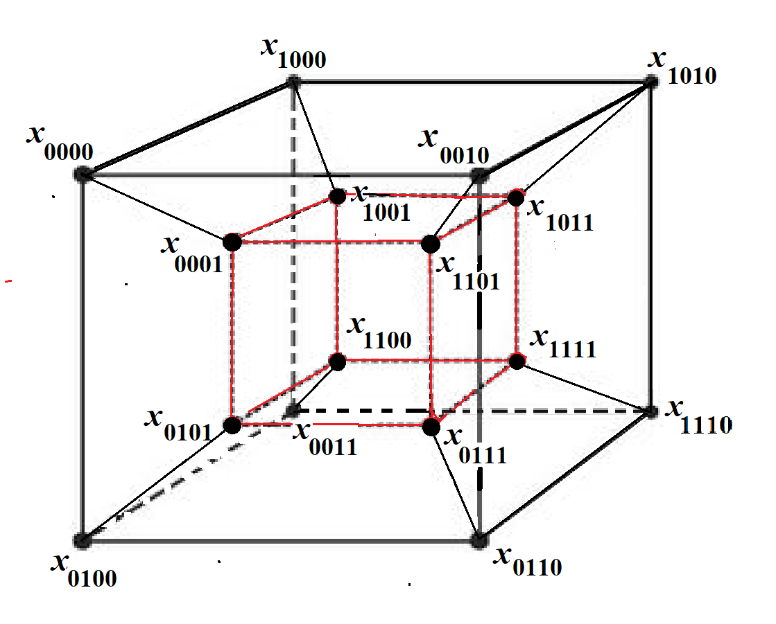
Figure 1: The $2^{4}$-tensors.

Symmetric $2^{4}$-tensors

If we want to consider symmetric $2^{4}$-tensors (sometimes called supersymmetric in the literature), those are given by the subspace, in the space $\mathbb{P}^{15}$ parameterizing all tensors, which is defined by the symmetry relations: $x_{ijkl}=x_{\sigma(ijkl)}$, for all $\sigma\in\mathfrak{S}_{4}$. The space parameterizing those tensors is a $\mathbb{P}^{4}$; if we use coordinates $\{y_{ijkl}\}$ in it, the variety parameterizing tensor of symmetric rank 1 is the Veronese variety $V_{4}$ (a rational normal curve), the image of the $4-ple$ embedding of $\mathbb{P}^{1}$:

$$[s_{0},s_{1}]\rightarrow[s_{0}^{4},s_{0}^{3}s_{1},s_{0}^{2}s_{1}^{2},s_{0}s_{1}^{3},s_{1}^{4}]$$

which can also be viewed as what we obtain when in the Segre map we have seen before we identify the four copies of $\mathbb{P}^{1}$, with $s_{i}=t_{i}=u_{i}=v_{i}$, $i=0,1$. The tensors we are considering now can be viewed in the next figure:

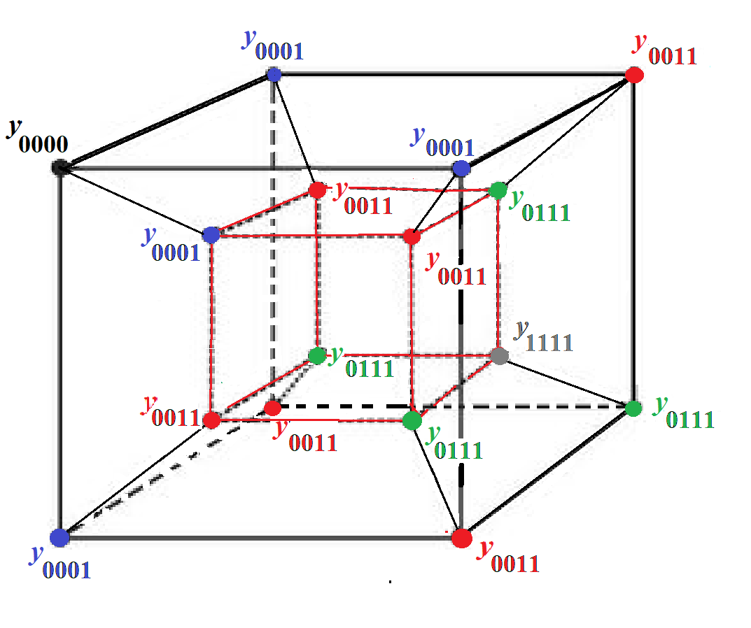
Figure 2: The symmetric $2^{4}$-tensors, the colors of the dots signal equal coordinates.

As it is well-known, $V_{4}$ is given by parametric equations $y_{ijkl}=s_{i}s_{j}s_{k}s_{l}$ (symmetric on $ijkl$) and its ideal is generated by all the $2\times 2$-minors of the tensor. Those minors can also be viewed either in the (1,3)-catalecticant or in the $(2,2)$-catalecticant matrices for forms of degree 4 in 2 variables:

$$\left(\begin{array}[]{cccc}y_{0000}&y_{0001}&y_{0011}&y_{0111}\cr y_{0001}&y_{0011}&y_{0111}&y_{1111}\end{array}\right)\quad,\quad\left(\begin{array}[]{ccc}y_{0000}&y_{0001}&y_{0011}\cr y_{0001}&y_{0011}&y_{0111}\cr y_{0011}&y_{0111}&y_{1111}\end{array}\right)$$

Partially Symmetric $2^{4}$-tensors

When considering the Segre-Veronese variety $V_{2,2}\subset\mathbb{P}^{8}$ defined above, it can be viewed as given first by the 2-ple Veronese embedding of both the $\mathbb{P}^{1}$-factors into $\mathbb{P}^{2}$, followed by the Segre embedding $\nu_{1,1}:\mathbb{P}^{2}\times\mathbb{P}^{2}\rightarrow\mathbb{P}^{8}$. Moreover, this space $\mathbb{P}^{8}$ parameterizes $2^{4}$-tensors which are symmetric on the first two indices and on the second two; namely we can see these partially symmetric tensors as the subspace ($\cong\mathbb{P}^{8}$) of the space of general $2^{4}$-tensors ($\cong\mathbb{P}^{15}$) with entries $x_{i_{0},i_{1},u_{0},u_{1},j_{0},j_{1},v_{0},v_{1}}$ defined by the equations $x_{i_{0},i_{1},u_{0},u_{1},j_{0},j_{1},v_{0},v_{1}}=x_{\sigma((i_{0},i_{1}),(u_{0},u_{1})),\tau((j_{0},j_{1}),(v_{0},v_{1})}$, for all $\sigma,\tau\in\mathfrak{S}_{2}$. We can view the partially symmetric $2^{4}$-tensors in the following figure. Notice that the four $2\times 2$ faces moving from left to right are symmetric and so are the four $2\times 2$ faces joining the “big cube” to the “small one” in the direction “perpendicular to the paper”

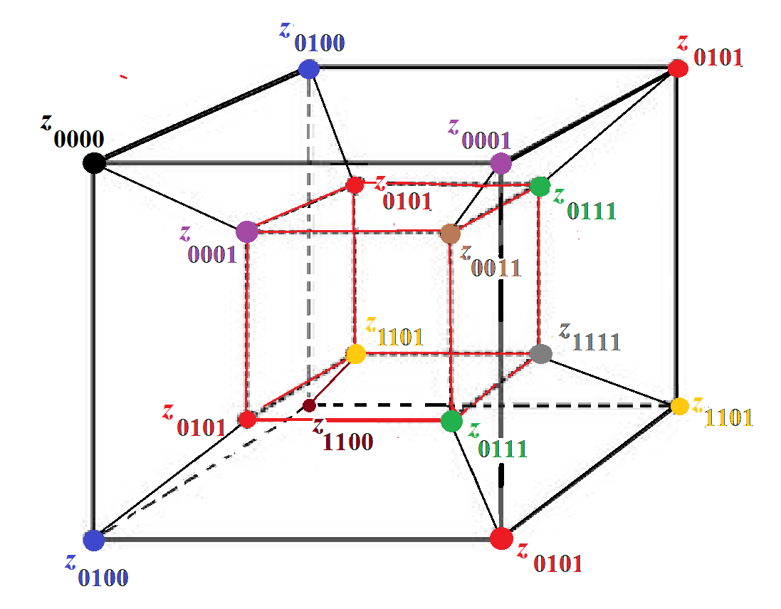
Figure 3: The Partially symmetric $2^{4}$-tensors.

We have that $V_{2,2}$ is a particular Del Pezzo surface, of degree 8 in $\mathbb{P}^{8}$ (e.g. see [CGG2]), its ideal is defined by the $2\times 2$ minors of the matrix

$$\left(\begin{array}[]{cccc}z_{0000}&z_{0001}&z_{0100}&z_{0101}\cr z_{0001}&z_{0011}&z_{0101}&z_{0111}\cr z_{0100}&z_{0101}&z_{1100}&z_{1101}\cr z_{0101}&z_{0111}&z_{1101}&z_{1111}\end{array}\right)$$

The matrix above gives the ideal of $V_{2,2}$ with its $2\times 2$-minors; moreover its $3\times 3$-minors generate its secant variety, $\sigma_{2}(V_{2,2})$, which has the expected dimension =5, while its determinant defines $\sigma_{3}(V_{2,2})$, which is defective, its expected dimension was 8 ( e.g. see again [CGG2]).

The generators of $I_{V_{2,2}}$ can also be viewed as the $(2\times 2)-$minors of the array above.

Notation The partially symmetric tensor rank $psrk(T)$ of a point $T\in\mathbb{P}^{8}$ is the $V_{2,2}-rank$ of $T$.

5.3 The variety $q_{2}(V_{2,2})$

Now let us go back to the $2$-square schemes we defined in $\mathbb{P}^{1}\times\mathbb{P}^{1}$; we considered a scheme $Q_{P}$ for every point $P\in\mathbb{P}^{1}\times\mathbb{P}^{1}$; under the Segre-Veronese embedding whose image is $V_{2,2}\subset\mathbb{P}^{8}$, each of these schemes, which we will denote $Q^{\prime}_{P}$, is such that $\langle Q^{\prime}_{P}\rangle\cong\mathbb{P}^{3}$. Here we will consider the variety

$$q_{2}(V_{2,2})=\overline{\bigcup_{P\in\mathbb{P}^{1}\times\mathbb{P}^{1}}\langle Q^{\prime}_{P}\rangle}$$

In order to visualize what $\langle Q^{\prime}_{P}\rangle$ is, recall that we defined $I_{Q_{P}}=(\ell_{s}^{2},\ell_{t}^{2})\subset R=\mathbb{C}[s_{0},s_{1};t_{0},t_{1}]$; let $m_{s}=as_{0}+bs_{1}\in R_{1,0}$ and $m_{t}=ct_{0}+dt_{1}\in R_{0,1}$, those are the elements of bidegree (1,0) and (0,1) such that $m_{s}\perp\ell_{s}$, $m_{t}\perp\ell_{t}$, with respect to the apolar action of the ring on itself via derivations (notice that we can have $m_{s}=\ell_{s}$ or $m_{t}=\ell_{t}$ for isotropic forms). We have that:

$(I_{Q_{P}})_{(2,2)}=\ell_{s}^{2}R_{0,2}+\ell_{t}^{2}R_{2,0}$, so that:

$(I^{\perp}_{Q_{P}})_{(2,2)}=m_{s}m_{t}R_{1,1}\cong\ \langle Q^{\prime}_{P}\rangle$.

Let us consider for example $P=[0,1;0,1]$, then $I_{Q_{P}}=(s_{0}^{2},t_{0}^{2})$ and

$$(I^{\perp}_{Q_{P}})_{(2,2)}=\langle s_{0}s_{1}t_{0}t_{1},s_{0}s_{1}t_{1}^{2},s_{1}^{2}t_{0}t_{1},s_{1}^{2}t_{1}^{2}\rangle,$$

hence the tensors in any $\langle Q^{\prime}_{P}\rangle$ can be written, modulo a bilinear change of coordinates in $\mathbb{P}^{1}\times\mathbb{P}^{1}$, as described in the next figure:

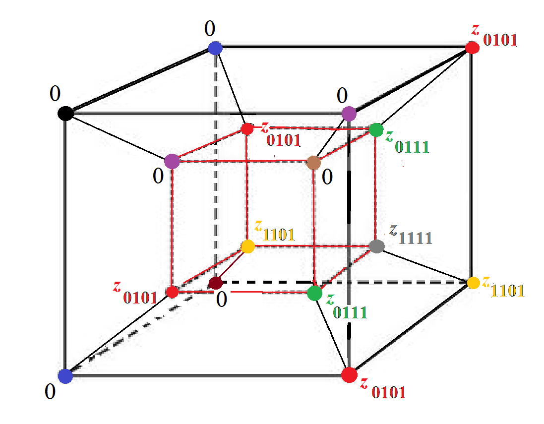
Figure 4: Tensors in $\langle Q^{\prime}_{P}\rangle$

Hence $\langle Q^{\prime}_{P}\rangle$ is defined by equations $z_{i_{0}i_{1}j_{0}j_{i}}=0$, for all $z_{i_{0}i_{1}j_{0}j_{i}}$ where either both $i$’s or both $j$’s are 0. Notice that since $\langle Q^{\prime}_{P}\rangle=\mathbb{P}(m_{s}m_{t}R_{1,1})$, while $\tau_{1,\nu_{22}(P)}=\mathbb{P}\langle m_{s}m_{t}(m_{s}R_{0,1}+m_{t}R_{1,0})\rangle$, we have $\tau_{1}(V_{2,2})\subset q_{2}(V_{2,2})$.

Now we want to consider the secant variety of $q_{2}(V_{2,2})$; namely we want to prove the following.

Proposition 5.1

We have that $\dim q_{2}(V_{2,2})=5$ and $\sigma_{2}(q_{2}(V_{2,2}))=\mathbb{P}^{8}$, as expected. Hence the generic partially symmetric tensor in $\mathbb{P}^{8}$ can be written as the sum of two p.s. tensors which depends only on four parameters each (and can be written, not at the same time, as in Fig. 4).

Proof To give a point in $\langle Q^{\prime}_{P}\rangle=\mathbb{P}^{3}\subset\mathbb{P}^{8}$ amounts to choosing a form $m_{s}m_{t}n_{s,t}$, with $m_{s}\in R_{1,0}$, $m_{t}\in R_{0,1}$, $n_{s,t}\in R_{1,1}$. Hence, in order to find the tangent space to $q_{2}(V_{2,2})$ at the point $m_{s}m_{t}n_{s,t}$, we have to consider another generic point $u_{s}u_{t}v_{s,t}\in q_{2}(V_{2,2})$, and then compute (e.g. see [CGG], [CGG1]):

$$\lim_{\lambda\rightarrow 0}\frac{d}{d\lambda}\left[(m_{s}+\lambda u_{s})(m_{t}+\lambda u_{t})(n_{s,t}+\lambda v_{s,t})\right]=$$

$$=u_{s}m_{t}n_{s,t}+m_{s}u_{t}n_{s,t}+m_{s}m_{t}n_{s,t}\subset R_{2,2}.$$

As $u_{s},u_{t},v_{s,t}$ vary, we get that the affine cone on the tangent space that we considered is:

$$W=m_{s}m_{t}R_{1,1}+m_{s}n_{s,t}R_{0,1}+m_{t}n_{s,t}R_{1,0}.$$

We have dim $W$ = 6 (affine), as expected. If we consider the ideal $I=(m_{s}m_{t},m_{s}n_{s,t},m_{t}n_{s,t})$, we have that $W=I_{2,2}$, and $I$ is the ideal of three points $P_{1},P_{2},P_{3}\in\mathbb{P}^{1}\times\mathbb{P}^{1}$; since they can be defined by $(m_{s},n_{s,t})$, $(m_{t},n_{s,t})$ and $(m_{s},m_{t})$, respectively, the three of them are not contained in a fiber, but $P_{1},P_{3}$ and $P_{2},P_{3}$ are (see Fig. 5a).

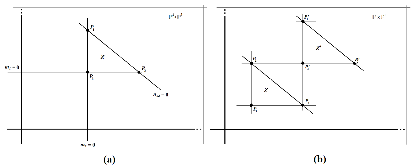
Figure 5: (a) $P_{1},P_{2},P_{3}$ in $\mathbb{P}^{1}\times\mathbb{P}^{1}$; (b) $Z\cup Z^{\prime}$ specialized.

We just have to consider two tangent spaces to $q_{2}(V_{2,2})$ at two generic points of $q_{2}(V_{2,2})$ (say given by $m_{s}m_{t}n_{s,t}$ and $u_{s}u_{t}v_{s,t}$); if their affine cones are $W$ and $W^{\prime}$, the (affine) space $W+W^{\prime}$ will give the tangent cone at a generic point of $\sigma_{2}(q_{2}(V_{2,2}))$, by Terracini’s Lemma. Since $W=(I_{Z})_{2,2}$ and $W^{\prime}=(I_{Z^{\prime}})_{2,2}$, where $Z$ and $Z^{\prime}$ are given by two configuration of three simple points as in Fig. 5a, $W\cap W^{\prime}$ is the $(2,2)$ part of the ideal of $Z\cup Z^{\prime}$.

Claim Let $Z,Z^{\prime}\subset\mathbb{P}^{1}\times\mathbb{P}^{1}$ be two schemes of three points, both positioned as in Fig. 5a. Then they impose independent conditions to forms of bidegree $(2,2)$, i.e. $\dim(I_{Z^{\prime}\cup Z})_{2,2}=3$.

Proof of Claim We can specialize $Z^{\prime}$ (see Fig. 5b) so that the line $u_{s}=0$ contains $P^{\prime}_{3}$, $P^{\prime}_{1}$ and also a point (say $P_{2}$) of $Z$; this forces the forms in $(I_{Z^{\prime}\cup Z})_{2,2}$ to be of type $u_{s}F$, with $F\in R_{1,2}$; now we have also that $F$, since $\{F=0\}$ contains $P_{1}$ and $P^{\prime}_{2}$, has to be of type $F=u_{t}G$, with $G\in R_{1,1}$ and $P_{3}\in\{G=0\}$. Hence $\dim(I_{Z^{\prime}\cup Z})_{2,2}=\dim(I_{P_{3}})_{1,1}=3$.

 

By the claim we get $\dim(W\cap W^{\prime})=\dim(I_{Z\cup Z^{\prime}})_{2,2}=3$, so $\dim(W+W^{\prime})=\dim W+\dim W^{\prime}-\dim(W\cap W^{\prime})=6+6-3=9$, and $\sigma_{2}(q_{2}(V_{2,2}))=\mathbb{P}^{8}$.

 

5.4 The varieties $V_{d,d}$ and their $q_{2}(V_{d,d})$, $d\geq 3$.

Now we want to generalize what we did to the case of Segre-Veronese varieties $V_{d,d}=\nu_{d,d}(\mathbb{P}^{1}\times\mathbb{P}^{1})\subset\mathbb{P}^{(d+1)^{2}-1}$, with $d\geq 3$. Also in this case $V_{d,d}$ parameterizes partially symmetric $2^{2d}-$tensors; we can define $q_{2}(V_{d,d})$ exactly as before and we have:

Proposition 5.2

For all $d\geq 3$, dim $q_{2}(V_{d,d})=5$ and dim $\sigma_{2}(q_{2}(V_{d,d}))=11$, as expected.

Proof We consider the variety $V_{d,d}\subset\mathbb{P}^{(d+1)^{2}-1}$, given by the Segre-Veronese embedding $\nu_{d,d}$, associated to the very ample line bundle $\mathcal{O}_{\mathbb{P}^{1}\times\mathbb{P}^{1}}(d,d)$; here $\mathbb{P}^{(d+1)^{2}-1}\subset\mathbb{P}^{2^{2d}-1}$, parameterizes the $2^{2d}$-tensors which are partially symmetric in the sense that each $z_{i_{1},\ldots,i_{d},i_{d+1},\ldots,i_{2d}}=z_{\sigma(i_{1},\ldots,i_{d}),\sigma^{\prime}(i_{d+1},\ldots,i_{2d})}$, for all $\sigma,\sigma^{\prime}\in\mathfrak{S}_{d}$. The variety $V_{d,d}$ parameterizes the partially symmetric $2^{2d}-$tensors $T$ with $psrkT=1$; as in the case $d=2$, the partially symmetric tensor rank $psrk(T)$ of a point $T\in P^{(d+1)^{2}-1}$ is the $V_{d,d}$-rank of $T$.

We want to consider the variety $q_{2}(V_{d,d})$, given by all the $2$-squares $Q_{P}$ defined by ideals $(\ell_{s}^{2},\ell_{t}^{2})$ and their images $Q_{P}^{\prime}\subset V_{d,d}$. Here $\langle Q^{\prime}_{P}\rangle$ will correspond to the linear space given by

$$(I^{\perp}_{Q_{P}})_{d,d}=m_{s}^{d-1}m_{t}^{d-1}R_{1,1}=(m_{s}^{d-1}m_{t}^{d-1})_{d,d}.$$

Hence, in order to find the tangent space to $q_{2}(V_{d,d})$ at the point corresponding to $m_{s}^{d-1}m_{t}^{d-1}n_{s,t}$, we have to consider another generic point $u_{s}^{d-1}u_{t}^{d-1}v_{s,t}\in q_{2}(V_{d,d})$, and then to compute:

$$\lim_{\lambda\rightarrow 0}\frac{d}{d\lambda}\left[(m_{s}+\lambda u_{s})^{d-1}(m_{t}+\lambda u_{t})^{d-1}(n_{s,t}+\lambda v_{s,t})\right]=$$

$$=(d-1)m_{s}^{d-2}u_{s}m_{t}^{d-1}n_{s,t}+(d-1)m_{t}^{d-2}u_{t}m_{s}^{d-1}n_{s,t}+m_{s}^{d-1}m_{t}^{d-1}v_{s,t}.$$

This, as $u_{s},u_{t},v_{s,t}$ vary, gives the space

$$W=(m_{s}^{d-1}m_{t}^{d-1},m_{s}^{d-1}m_{t}^{d-2}n_{s,t},m_{s}^{d-2}m_{t}^{d-1}n_{s,t})_{d,d}\subset(I_{Z})_{d,d}$$

where $Z$ is the scheme given by $I_{Z}=(m_{s}^{d-1}m_{t}^{d-1},m_{s}^{d-1}m_{t}^{d-2}n_{s,t},m_{s}^{d-2}m_{t}^{d-1}n_{s,t})$ and $Z$ is a scheme which is made of the two lines $m_{s}=0$, $m_{t}=0$, both with multiplicity $d-2$, plus two $(d-1)$-jets on $\{n_{s,t}=0\}$, supported at the points given by $(m_{s},n_{s,t})$ and $(n_{s,t},m_{t})$ (see Fig. 6). We have that $W$ has (vector) $dimW=6$, as expected, while $dim(I_{Z})_{d,d}=7$ (all forms in $(I_{Z})_{d,d}$ are of type $m_{s}^{d-2}m_{t}^{d-2}F$, where $F$ is a $(2,2)-$form passing through the two points where the jets are, hence $dim(I_{Z})_{d,d}=9-2=7$).

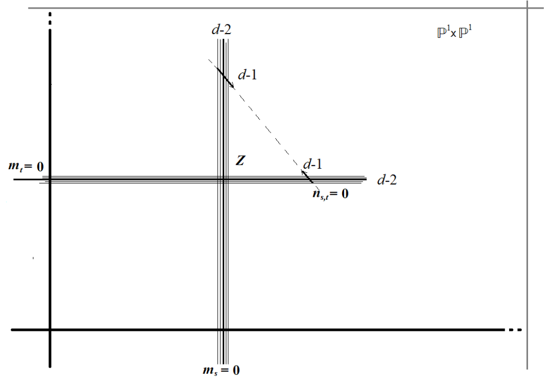
Figure 6: The scheme given by two $(d-2)-$ple lines with two $(d-1)$-jets sprouting from them.

By Terracini’s Lemma, we just have to consider two tangent spaces to $q_{2}(V_{d,d})$ at two generic points of $q_{2}(V_{d,d})$; if their affine cones are $W$ and $W^{\prime}$, the (vector) space $W+W^{\prime}$ will be the tangent cone to a generic point of $\sigma_{2}(q_{2}(V_{3,3}))$. Since $W\subset(I_{Z})_{d,d}$ and $W^{\prime}\subset(I_{Z^{\prime}})_{d,d}$, where $Z$ and $Z^{\prime}$ will be made as in Fig. 6 (two $(d-2)-$lines with two $(d-1)-$jets), $W\cap W^{\prime}\subset(I_{Z})_{d,d}\cap(I_{Z^{\prime}})_{d,d}=(I_{Z\cup Z^{\prime}})_{d,d}$. We want to check that $(I_{Z\cup Z^{\prime}})_{d,d}=\{0\}$.

Case $d=3$. Since the forms in $(I_{Z\cup Z^{\prime}})_{3,3}$ should contain the factor $m_{s}m_{t}m^{\prime}_{s}m^{\prime}_{t}\in R_{2,2}$, and no form in $R_{1,1}$ passes through the four points which are the support of the four jets, we get $(I_{Z\cup Z^{\prime}})_{3,3}=\{0\}$.

Case $d\geq 4$. Forms in $(I_{Z\cup Z’})_{d,d}$ should contain the factor $m_{s}^{d-2}m_{t}^{d-2}m_{s}^{\prime d-2}m_{t}^{\prime d-2}$, which is impossible for $d\geq 5$, while for $d=4$ there would be only this form, which does not contain the four $d-1$ jets at the four points $m_{s}\cap n_{s,t}$ , $m_{t}\cap n_{s,t}$ , $m’_{s}\cap n^{\prime}_{s,t}$ , $m’_{t}\cap n^{\prime}_{s,t}$, hence also in this case $(I_{Z\cup Z^{\prime}})_{3,3}=\{0\}$, which in turn implies that $W\cap W^{\prime}=\{0\}$.

Now, from Grassmann equality, we get $\dim(W+W^{\prime})=\dim W+\dim W^{\prime}-\dim(W\cap W^{\prime})=6+6-0$, hence $\dim(W+W^{\prime})=12$ (as vector space) and $\dim\sigma_{2}(q_{2}(V_{3,3}))=11$.

 

5.5 The cuckoo varieties $qq_{2}(V_{d,d})$

As we have done in the Veronese case, here too we are going to define a “cuckoo variety” inside $q_{2}(V_{d,d})$, which could also have some interest in relation to Quantum Entanglement. If we consider the Hilbert space of a composite quantum system, then this is the tensor product of the Hilbert spaces of the constituent systems, and tensor rank is a natural measure of the entanglement for the corresponding quantum states. The Hilbert space of a $k$-body system is obtained as the tensor product of $k$ copies of the single particle Hilbert space ${\mathcal{H}}_{1}$. In the case of indistinguishable bosonic particles, the totally symmetric states under particle exchange are physically relevant, which amounts to restricting the attention to the subspace $H_{s}=S^{N}({\mathcal{H}}_{1})\subset{\mathcal{H}}_{1}^{\otimes N}$ of symmetric tensors.

In case we have $k\geq 2$ different species of indistinguishable bosonic particles, the relevant Hilbert space is $S^{N_{1}}({\mathcal{H}}_{1})\otimes S^{N_{2}}({\mathcal{H}}_{2})\otimes\ldots\otimes S^{N_{k}}({\mathcal{H}}_{2})$. Of particular interest, in physics literature, are the so-called $W$-states, i.e. quantum entangled states that can be expressed in Dirac notation as:

$${\displaystyle|\mathrm{W}\rangle={\frac{1}{\sqrt{n}}}(|100...0\rangle+|010...0\rangle+...+|00...01\rangle).}$$

Which, if ${\mathcal{H}}_{1}=\mathbb{C}^{2}$ with coordinates $(x,y)$, can be written as:

$$W_{d}=y\otimes x\otimes\ldots\otimes x+x\otimes y\otimes x\otimes\ldots\otimes x+x\otimes x\otimes\ldots\otimes y.$$

When treating with bosonic particles, hence with symmetric tensors, $W_{d}$ can be represented simply as a monomial $x^{d-1}y$, hence in the study of entanglement of $k$ different $d$-body systems (made of different species of indistinguishable bosonic particles, like photons), we can consider the product of $k$ $W_{d}$ states: $W_{d}\otimes\ldots\otimes W_{d}$, where each $W_{d}\cong x^{d-1}y\in S^{d}\mathbb{C}^{2}\subset(\mathbb{C}^{2})^{\otimes d}$ (e.g. see [BBCG]).

In [BBCG], Lemma 2.1, it is proved that $W_{d}\otimes\ldots\otimes W_{d}\in\langle\nu_{d,\ldots,d}(Z)\rangle$, where $Z$ is a $2-$hypercube in $\mathbb{P}^{1}\times\ldots\times\mathbb{P}^{1}$, and this is expressed by saying that the cactus rank of $W_{d}\otimes W_{d}$ is $2^{k}$ and it is realized by $Z$ (the cactus rank of a tensor $T\in\mathbb{P}^{(d+1)^{k}-1}$ is the minimum lenght of a $0-$dimensional scheme $X\subset V_{d,\ldots,d}$ such that $T\in\langle X\rangle$). We can improve a bit that lemma in this setting (in [BBCG] also the case of $W_{d_{1}}\otimes\ldots\otimes W_{d_{k}}$ is considered, with different $d_{i}$’s):

Corollary 5.3

Let $T\in P^{(d+1)^{k}-1}$ parameterize $W_{d}\otimes\ldots\otimes W_{d}$; then the smoothable rank of $T$ is $smrk=2^{k}$.

Proof The only difference between smoothable rank and cactus rank is that $smrk\ T=r$ if and only if there is a smoothable $0-$dimensional scheme $X\subset V_{d,\ldots,d}$ such that $T\in\langle X\rangle$ and $\ell(X)=r$. Since, by Proposition 2.11, any $2-$hypercube is smoothable, the statement is an immediate consequence of this and of Lemma 2.1 of [BBCG], since for any tensor the smoothable rank is greater or equal than the cactus rank.

 

Let us consider the case $k=2$; $q_{2}(V_{d,d})$ parameterizes partially symmetric tensors in the spaces:

$$<\nu_{d,d}(Q_{P})>=(m_{s}^{d-1}m_{t}^{d-1})_{d,d}$$

Hence for all tensors of type $W_{d}\otimes W_{d}=m_{s}^{d-1}a_{s}m_{t}^{d-1}b_{t}$, $m_{s},a_{s}\in R_{1,0}$, $m_{t},b_{t}\in R_{0,1}$, we have $W_{d}\otimes W_{d}\in<\nu_{d,d}(Q_{P})>$, for some $P\in\mathbb{P}^{1}\times\mathbb{P}^{1}$.

More specifically, let us consider the subvariety which parameterizes exactly the tensors of type $W_{d}\otimes W_{d}$:

Definition 5.4

The cuckoo variety $qq_{2}(V_{d,d})\subset q_{2}(V_{d,d})$ is the image of the map:

$$\mathbb{P}^{1}\times\mathbb{P}^{1}\times\mathbb{P}^{1}\times\mathbb{P}^{1}=\mathbb{P}(\mathbb{C}[s_{0},s_{1}]_{1})\times\mathbb{P}(\mathbb{C}[s_{0},s_{1}]_{1})\times\mathbb{P}(\mathbb{C}[t_{0},t_{1}]_{1})\times\mathbb{P}(\mathbb{C}[t_{0},t_{1}]_{1})\rightarrow q_{2}(V_{d,d})\subset\mathbb{P}^{8},$$

with: $(m_{s},n_{s},m_{t},n_{t})\rightarrow m_{s}^{d-1}n_{s}m_{t}^{d-1}n_{t}$.

We have that $qq_{2}(V_{d,d})$ has dimension 4, and, via a multi-linear change of coordinates, every form parameterized by a point in $qq_{2}(V_{d,d})$ can be written as a monomial $s_{0}^{d-1}s_{1}t_{0}^{d-1}t_{1}$ (for results on the various ranks of such monomials see [CF],[Ga] and [BBCG]). We have :

Proposition 5.5

$qq_{2}(V_{d,d})$ is such that:

i) $\forall P\in\mathbb{P}^{1}\times\mathbb{P}^{1}$, $qq_{2}(V_{d,d})\cap\langle Q^{\prime}_{P}\rangle\cong\mathcal{Q}_{P}$, where $\mathcal{Q}_{P}$ is a smooth quadric in $\langle Q^{\prime}_{P}\rangle\cong\mathbb{P}^{3}$.

ii) $\forall P\in\mathbb{P}^{1}\times\mathbb{P}^{1}$, we have $\tau_{1,\nu_{dd}(P)}(\mathcal{Q}_{P})=\tau_{1,\nu_{dd}(P)}(V_{dd})$.

iii) $Sing(qq_{2}(V_{d,d}))$ is the locus of forms of type $m_{s}^{d}m_{t}^{d-1}n_{t}$ or $m_{s}^{d-1}n_{s}m_{t}^{d}$.

Proof As we have seen, if $\nu_{d,d}(P)=m_{s}^{d}m_{t}^{d}$, then we can write

$$\langle Q^{\prime}_{P}\rangle=(m_{s}^{d-1}m_{t}^{d-1})_{d,d}=m_{s}^{d-1}m_{t}^{d-1}R_{1,1},$$

where $n_{s},n_{t}$ are such that $R_{1,0}=\langle m_{s},n_{s}\rangle$, $R_{0,1}=\langle m_{t},n_{t}\rangle$ and $R_{1,1}=\langle m_{s}m_{t},m_{s}n_{t},n_{s}m_{t},n_{s}n_{t}\rangle$. Hence any points in $\langle Q^{\prime}_{P}\rangle$ corresponds (modulo constants) to a form of type $am_{s}m_{t}+bm_{s}n_{t}+cn_{s}m_{t}+dn_{s}n_{t}$, i.e. we can view $\langle Q^{\prime}_{P}\rangle\cong\mathbb{P}(R_{1,1})$, and in it the forms of type $a_{s}a_{t}$, for $a_{s}\in R_{1,0}$, $a_{t}\in R_{0,1}$, are precisely parametrized by a quadric $\mathcal{Q}_{P}$ which is the Segre Variety $V_{11}$; $\mathcal{Q}_{P}$ is given exactly by the forms for which $ad-bc=0$. This proves part i).

To prove part ii), just notice that $\tau_{1,\nu_{dd}(P)}(V_{dd})$ is given by the forms in $m_{s}^{d-1}m_{t}^{d-1}(m_{s}R_{0,1}+m_{t}R_{1,0})$, hence $\mathcal{Q}_{P}\cap\tau_{1,\nu_{dd}(P)}(V_{dd})$ is given by the forms of type either $m_{s}^{d}m_{t}^{d-1}(\alpha_{t}+m_{t})$ or $m_{s}^{d-1}(m_{s}+\beta_{s})m_{t}^{d}$, which gives two lines in $\tau_{1,\nu_{dd}(P)}(V_{dd})$, hence this is the tangent plane to $\mathcal{Q}_{P}$ in $\langle Q^{\prime}_{P}\rangle$.

In order to prove iii), let us consider the affine cone $W$ over the tangent space of $qq_{2}(V_{d,d})$ at one of its points, say the one associated to $m_{s}^{d-1}n_{s}m_{t}^{d-1}n_{t}$; if we consider another point $u_{s}^{d-1}v_{s}u_{t}^{d-1}v_{t}$, we have to compute:

$$\lim_{\lambda\rightarrow 0}\frac{d}{d\lambda}\left[(m_{s}+\lambda u_{s})^{d-1}(n_{s}+\lambda v_{s})(m_{t}+\lambda u_{t})^{d-1}(n_{s}t+\lambda v_{t})\right]=$$

$$=\langle(d-1)m_{s}^{d-2}u_{s}n_{s}m_{t}^{d-1}n_{t}+m_{s}^{d-1}v_{s}m_{t}^{d-1}n_{t}+(d-1)m_{s}^{d-1}n_{s}m_{t}^{d-2}u_{t}n_{t}+m_{s}^{d-1}n_{s}m_{t}^{d-1}v_{t}\rangle.$$

Hence, as $u_{s},v_{s},u_{t},v_{t}$ vary, we get

$$W\cong\langle m_{s}^{d-2}m_{t}^{d-2}\left(m_{s}m_{t}(R_{1,0}n_{t}+n_{s}R_{0,1})+n_{s}n_{t}(R_{1,0}m_{t}+m_{s}R_{0,1})\right)\rangle\subset R_{d,d}.$$

Generically, we have $\dim_{\mathbb{C}}(R_{1,0}a_{t}+a_{s}R_{0,1})=3$, since they have $\langle a_{s}a_{t}\rangle$ in common, hence $W$ is the sum of two subspaces of (affine) dimension 3, which have $\langle m_{s}^{d-1}n_{s}m_{t}^{d-1}n_{t}\rangle$ in common, so $\dim_{\mathbb{C}}W=5$, as expected.

The locus $Sing(qq_{2}(V_{d,d}))$ is given by the points where $\dim W<5$, and it is easy to check that this happens for either $m_{s}=n_{s}$ or $m_{t}=n_{t}$, and this proves iii).

 

There is another way to view the variety $qq_{2}(V_{d,d})$; consider the embedding $\nu_{dd}(\mathbb{P}^{1}\times\mathbb{P}^{1})$ as the composition:

$$\mathbb{P}^{1}\times\mathbb{P}^{1}\rightarrow\mathbb{P}^{d}\times\mathbb{P}^{d}\rightarrow\mathbb{P}^{d^{2}+2d}$$

where the first arrow is $\nu_{d}\times\nu_{d}$ and the second is the Segre embedding $s_{1,1}$. If the image of the first map is $C_{d}^{s}\times C_{d}^{t}$, where $C_{d}^{s},C_{d}^{t}$ are the rational normal curves defined by $\mathbb{C}[s_{0},s_{1}]_{d},\mathbb{C}[t_{0},t_{1}]_{d}$, respectively, we can consider the product of their tangential varieties $\tau(C_{d}^{s})\times\tau(C_{d}^{t})\subset\mathbb{P}^{d}\times\mathbb{P}^{d}$, parameterizing pairs of forms like $(m_{s}^{d-1}a_{s},m_{t}^{d-1}a_{t})$; so $s_{1,1}(\tau(C_{d}^{s})\times\tau(C_{d}^{t}))$ is exactly $qq_{2}(V_{d,d})$.

We know that the singular locus of the tangential surface to a rational normal curve is the rational normal curve itself, hence $Sing(\tau(C_{d}^{s})\times\tau(C_{d}^{t}))=(\tau(C_{d}^{s})\times C_{d}^{t})\cup(C_{d}^{s}\times\tau(C_{d}^{t}))$, in correspondence with what we saw in Prop. 5.5, iii).

Notice that for $d=2$, we have: $qq_{2}(V_{2,2})=s_{1,1}(\tau(C^{s}_{2})\times\tau(C^{t}_{2}))=s_{1,1}(\mathbb{P}^{2}\times\mathbb{P}^{2})$, hence $qq_{2}(V_{2,2})$ is just the Segre Variety $S=s_{1,1}(\mathbb{P}^{2}\times\mathbb{P}^{2})\subset\mathbb{P}^{8}$, which is well known to be $2-$defective (it is the variety of $3\times 3$ matrices of rank 2), i.e. dim $\sigma_{2}(S)=7$.

We want to check that this does not happen for $d\geq 3$, i.e.

Proposition 5.6

For $d\geq 3$, $\dim\sigma_{2}(qq_{2}(V_{2,2}))=9$, as expected.

Proof By Terracini’s Lemma the dimension of the affine tangent cone at a generic point of $\sigma_{2}(qq_{2}(V_{d,d}))$ will be $\dim W_{1}+W_{2}$, where $W_{1}$, $W_{2}$ are the affine tangent cones at two generic points of $qq_{2}(V_{d,d})$. Thus, in order to prove our statement, we have to show that $\dim(W_{1}+W_{2})=10$, i.e. since $\dim W_{1}=\dim W_{2}=5$, that $W_{1}\cap W_{2}=\{0\}$.

In the proof of Prop. 5.5, iii), we have computed the affine tangent cone $W$ at a generic point of $qq_{2}(V_{2,2})$, hence if we pick two generic points given by forms: $m_{s}^{d-1}n_{s}m_{t}^{d-1}n_{t}$ and $u_{s}^{d-1}v_{s}u_{t}^{d-1}v_{t}$, we will have:

$$W_{1}=\langle m_{s}^{d-2}m_{t}^{d-2}\left(m_{s}m_{t}n_{t}R_{1,0}+m_{s}m_{t}n_{s}R_{0,1}+n_{s}m_{t}n_{t}R_{1,0}+n_{s}m_{s}n_{t}R_{0,1}\right)\rangle\subset(m_{s}^{d-2}m_{t}^{d-2})R_{2,2},$$

$$W_{2}=\langle u_{s}^{d-2}u_{t}^{d-2}\left(u_{s}u_{t}v_{t}R_{1,0}+u_{s}v_{s}u_{t}R_{0,1}+v_{s}u_{t}v_{t}R_{1,0}+u_{s}v_{s}v_{t}R_{0,1}\right)\rangle\subset(u_{s}^{d-2}u_{t}^{d-2})R_{2,2}.$$

When $d\geq 5$ it is immediate to check that $W_{1}\cap W_{2}=\{0\}$, so we are done.

If $d=4$, then $(m_{s}^{d-2}m_{t}^{d-2})R_{2,2}\cap(u_{s}^{d-2}u_{t}^{d-2})R_{2,2}=\langle m_{s}^{2}m_{t}^{2}u_{s}^{2}u_{t}^{2}\rangle$ and it easy to check that $m_{s}^{2}m_{t}^{2}u_{s}^{2}u_{t}^{2}\notin W_{1}\cap W_{2}$ (it sufficies to consider $m_{s}=s_{0},m_{t}=t_{0},n_{s}=s_{1},n_{t}=t_{1}$ and notice that $s_{i}^{2}t_{j}^{2}\notin W_{1}$, while these monomials will appear in $u_{s}^{2}u_{t}^{2}$).

Eventually, for $d=3$, let $W_{1}=s_{0}t_{0}(s_{0}^{2},s_{0}s_{1}t_{0}t_{1},s_{0}s_{1}t_{0}^{2},s_{1}^{2}t_{0}t_{1},s_{0}s_{1}t_{1}^{2})$, if there is something not 0 in $W_{1}\cap W_{2}$ it should be of the form $s_{0}t_{0}u_{s}u_{t}n_{s,t}$, with $n_{s,t}\in R_{1,1}$, but since $u_{s},u_{t}$ are generic, say $u_{s}u_{t}=(as_{0}+bs_{1})(ct_{0}+bt_{1})$, in $u_{s}u_{t}n_{s,t}$ the monomials $s_{i}^{2}t_{j}^{2}$ should appear, and this is impossible since they are not in $\langle s_{0}^{2},s_{0}s_{1}t_{0}t_{1},s_{0}s_{1}t_{0}^{2},s_{1}^{2}t_{0}t_{1},s_{0}s_{1}t_{1}^{2}\rangle$. Hence $W_{1}\cap W_{2}=\{0\}$ also for $d=3$ and we are done.

 

Acknowledgements All the authors are members of GNSAGA of Indam. We would like to thank J. Buczyński for his several suggestions. The third author wants to thank the organizers of AGATES workshop “Geometry of secants”, Warsaw October 2022 (supported by the Simons Foundation, award number 663281, and by Institute of Mathematics of Polish Academy of Sciences) for the opportunities given by this useful initiative. In particular thanks to H. Abo, E.Ventura and E. Postinghel for useful talks.

Maria V. Catalisano, Scuola Politecnica - Università di Genova, mariavirginia.catalisano@unige.it

Stefano Canino, Dipartimento di Scienze Matematiche - Politecnico di Torino, stefano.canino@polito.it

Alessandro Gimigliano, Dipartimento di Matematica - Università di Bologna, alessandr.gimigliano@unibo.it

Monica Idà, Dipartimento di Matematica - Università di Bologna, monica.ida@unibo.it

References

- [BBCG] E.Ballico, A.Bernardi, M. Christandl, F. Gesmundo, On the partially symmetric rank of tensor products of W-states and other symmetric tensors. Atti della Accademia Nazionale dei Lincei, Classe di Scienze, Rendiconti Lincei Matematica E Applicazioni 30 (2018) DOI:10.4171/RLM/837, available at https://arxiv.org/abs/1803.01623
- [BF] E. Ballico, C.Fontanari, On the secant varieties to the osculating variety of a Veronese surface, Central Europ. J. of Math. 1 (2003), 315-326.
- [BCCGO] A.Bernardi, E. Carlini, M.V.Catalisano, A. Gimigliano, A. Oneto The hitchhiker guide to secant varieties and tensor decomposition. Mathematics 6 (2018, special issue: ”Decomposibility of Tensors”, L.Chiantini Ed.); DOI: 10.3390/math6120314. Also available at http://www.mdpi.com/2227-7390/6/12/314/pdf
- [BCGI] A.Bernardi, M.V.Catalisano, A.Gimigliano, M.Idà, Osculating Varieties of Veronesean and their higher secant varieties. Canadian J. of Math. 59, (2007), 488-502.
- [BCGI2] A.Bernardi, M.V.Catalisano, A.Gimigliano, M.Idà, Secant varieties to Osculating Varieties of Veronese embeddings of . J. of Algebra, 321, (2009), 982-1004 (available also at: http://arxiv.org/0807.2455v2)
- [BGI] A.Bernardi, A.Gimigliano, M.Idà, Computing symmetric rank for symmetric tensors. J. of Symbolic Computation, 46, (2011), 34–53 (available also at: http://arxiv.org/abs/0908.1651)
- [CGI] S.Canino, A.Gimigliano, M.Idà, On the Jacobian scheme of a plane curve Preprint (available at: https://arxiv.org/abs/2302.07042).
- [CCG] E Carlini,M.V.Catalisano, A.V.Geramita, The solution to the Waring problem for monomials and the sum of coprime monomials J. of Symbolic Computation, 54, (2013), 9–35.
- [CGG] M.V.Catalisano, A.V.Geramita, A.Gimigliano, Tensor rank, secant varieties to Segre varieties and fat points in multiprojective spaces. Lin. Alg. and Appl. 355, (2002) , 263-285. (see also the errata of the publisher: 367 (2003), 347-348).
- [CGG1] M.V.Catalisano, A.V.Geramita, A.Gimigliano, On the secant varieties to the tangential varieties of a Veronesean. Proc. Am. Math. Soc. 130, (2001), 975-985.
- [CGG2] M.V.Catalisano, A.V.Geramita, A.Gimigliano, On the ideals of Secant Varieties to certain rational varieties. J. of Algebra 319, (2008), 1913–1931 (also available at: arXiv:math/0609054).
- [CF] L. Chen and S. Friedland. The tensor rank of tensor product of two three-qubit W-states is eight. Linear Algebra and its Applications, 543, (2018), 1 – 16.
- [COCOA] J.Abbott, A.M.Bigatti, L.Robbiano, CoCoA: a system for doing Computations in Commutative Algebra. Available at http://cocoa.dima.unige.it
- [Fu2] W.Fulton, Intersection Theory. Springer-Verlag, Berlin, Heidelberg, New York, 1998.
- [Ga] M. Gałazka. Multigraded apolarity. Math. Nach., 296, (2023), 286–313.
- [Ge] A. Geramita, Inverse systems of fat points: Waring’s problem, secant varieties of Veronese varieties, and parameter spaces for Gorenstein ideals, in Queen’s Papers in Pure and Appl. Math. 102 (1996) 1-114.
- [Ha] B.Hartshorne, Algebraic Geometry. Springer, Grad. Texts in Math. 52, Berlin, Heidelberg, New York 1977.
- [I] A. Iarrobino, Inverse system of a symbolic power. III. Thin algebras and fat points.Composito Math. 108 (1997) 319-356.
- [J] J. Jelisiejew Hilbert schemes of points and their applications PhD dissertation, University of Warsaw (2017). https://arxiv.org/pdf/2205.10584.pdf
- [LT] J.M.Landsberg, Z.Teitler, On the ranks and border ranks of symmetric tensors. Found. Comput. Math. 10 (2010), 339–366.
- [Pu] M.Pucci, The Veronese Variety and Catalecticant Matrices, J.of Algebra 202 (1998) 72-95.
- [S] D.L. Sayers, The lost tools of learning. Speech at Oxford Univ. (1947), available at https://classicalchristian.org/the-lost-tools-of-learning-dorothy-sayers/?v=a44707111a05
- [Sy] E. D. Sylla, Sister Katrei and Gregory of Rimini: Angels, God and Mathematics in the Fourteen Century. In: Mathematics and the Divine: a Hystorical Study T.Koetsier, L. Bergmans (editors) (2005) Elsevier. Boston, Heidelberg, London.
- [TA] Thomas Aquinas Summa Theologica (1265-1274), First (partial) edition by P. Schoffler,1471, Meinz; First full edition by M. Wenssler, Basel,1485.