Abelian-Higgs cosmic strings: effective action and particle radiation

Abstract

We utilized the duality between massive vector and massive Kalb-Ramond fields to derive an effective action for Abelian-Higgs cosmic strings. This enabled us to determine the classically renormalized string tension and facilitate calculations for back-reaction effects. Additionally, we derived a comprehensive expression for the energy flux of radiation emitted by Abelian-Higgs cosmic strings. Applying this equation to a cuspless loop, we obtained that the loop lifetime is proportional to the square of the loop length, which is in agreement with field-theory simulations.

1 Introduction

Soliton-like solutions emerge in various field theory models, such as quantum chromodynamics, extensions of the standard model of particle physics, condensed matter, and high-energy physics of the early universe [1, 2, 3]. In the context of cosmology, the study of one-dimensional topological solitons, known as cosmic strings, holds significant interest due to their properties and their potential presence in different scenarios during the early stages of the universe [4, 5, 6, 7].

Understanding the dynamics of these non-linear objects is a difficult task. Hence, lattice field theory simulations are commonly employed as a computational tool. However, simulating cosmic strings evolving in the expanding universe presents particular difficulties, as the simulations must simultaneously capture the details of a tiny string core and the vast area of the Hubble volume. Numerous numerical approaches in field theory try to obtain realistic results in simulations that encompass such contrasting scales [8, 9, 10, 11, 12, 13], mostly relying on the simplest models that correspond to global and local U(1) symmetry breaking.

An alternative simulation method approximates cosmic strings as infinitely thin and describes them using a Nambu-Goto action [27, 28, 29, 30]. This approach enables more detailed simulations on a larger scale. Nevertheless, the reliability of this approximation remains uncertain as it neglects back-reaction and radiation inherent in the original field theory model. A recent numerical study comparing Nambu-Goto and Abelian-Higgs strings suggests that the discrepancy clearly arises in regions of strings with high curvature [31].

Accurate modeling of cosmic string dynamics and the evolution of their network is essential for accurate prediction of possible observational signals. Currently, gravitational lensing [32, 33, 34], anisotropies in the cosmic microwave background [35, 36, 38, 37, 39, 40] and the stochastic gravitational wave background [41, 42, 43, 44, 45] serve as the most sensitive probes for detecting the presence of cosmic strings. Such knowledge allows for constraints to be imposed on high-energy models of the early universe through topological defects [46, 47, 48, 49, 50].

In this paper, we focus our attention on local Abelian-Higgs cosmic strings. We organize our study as follows: In Section 2, we construct an effective action employing the duality between massive vector and massive Kalb-Ramond fields. This model yields a classically renormalized string tension and enables the calculation of back-reaction, which we present in Section 3. Section 4 discusses the description of massive radiation, focusing on the particular example of cuspless loops. We compare our findings with recent results on simulations of massive radiation from Abelian-Higgs strings [51, 52]. Finally, in Section 5, we conclude and propose further steps that may be of interest for the newly developed formalism.

Throughout the paper we define a 4-dimensional metric by $g_{\mu\nu}$ with the signature $(+,-,-,-)$, where all Greek indexes run over space-time dimensions. Latin indexes in the middle of the alphabet $(i,k,\dots)$ run over spatial coordinates, while the first letters $(a,b,c,d)$ run over 2-dimensional string worldsheet coordinates.

2 Effective model of Abelian-Higgs cosmic strings

It is known that the global U(1) cosmic string model can be represented effectively via Nambu-Goto action coupled to a massless Kalb-Ramond field [54, 53]. In this section, we demonstrate that similarly to global strings one can obtain that the local U(1) Abelian-Higgs strings are effectively described by Nambu-Goto action coupled to a massive Kalb-Ramond field.

2.1 Duality between massive vector and massive Kalb-Ramond fields

Let us consider the Abelian-Higgs model, which is given by the action

$$\mathcal{S}=\int\left(D_{\mu}\varphi\left(D^{\mu}\varphi\right)^{*}-\frac{1}{4}F^{\mu\nu}F_{\mu\nu}-\frac{\lambda}{2}(\eta^{2}-|\varphi|^{2})^{2}\right)\sqrt{-g}\;d^{4}x,$$ (2.1)

where $g$ is a metric determinant, $\lambda$ and $\eta$ define the shape of potential, $D_{\mu}=\nabla_{\mu}-ieA_{\mu}$ is the gauge covariant derivative, $A^{\mu}$ is electromagnetic 4-potential, $F_{\mu\nu}=\nabla_{\mu}A_{\nu}-\nabla_{\nu}A_{\mu}$ is electromagnetic tensor and $\nabla_{\mu}$ is a covariant derivative for curved space-time. According to the Kibble mechanism [55], the Lagrangian (2.1) can give rise to topological string-like defects. Perturbation of the action (2.1), around the minimum of potential $\left(\varphi=\eta+\frac{\varphi_{1}+i\theta}{\sqrt{2}}\right)$, leads to

$$\begin{gathered}\mathcal{S}=\int\left(\mathcal{L}_{\rm br}+\mathcal{L}_{\rm int}\right)\sqrt{-g}\;d^{4}x,\end{gathered}$$ (2.2)

where

$$\mathcal{L}_{\rm br}=\frac{1}{2}\partial_{\mu}\varphi_{1}\partial^{\mu}\varphi_{1}-\lambda\eta^{2}\varphi_{1}^{2}-\frac{1}{4}F^{\mu\nu}F_{\mu\nu}+e^{2}\eta^{2}\tilde{A}_{\mu}\tilde{A}^{\mu},$$

$\mathcal{L}_{\rm int}$ includes higher order terms of $\varphi_{1}$ and $A_{\mu}$ and the vector field $\tilde{A}_{\mu}=A_{\mu}-\frac{1}{\sqrt{2}e\eta}\partial_{\mu}\theta$ acquired mass $M=\sqrt{2}e\eta$. By adding a divergence term to the action (2.2) and using equations of motion for the Proca field, one can obtain Hamiltonian for the vector part of the action (2.2)

$$\mathcal{H}=-\pi^{\mu}\pi_{\mu}+M^{2}\tilde{A}_{0}^{2}-\mathcal{L}_{\rm br},$$ (2.3)

where $\pi^{\mu}=F^{\mu 0}$ is a canonical momentum. If there is no explicit time dependence in Hamiltonian, it is possible to carry out canonical transformations substituting $\mathcal{L}_{\rm br}(\tilde{A}_{\mu})$ by $\mathcal{L}_{\rm KR}(B_{\mu\nu})$ with the corresponding change of canonical coordinates $\tilde{A}_{\mu}\rightarrow B_{\mu\nu}$ and momenta $\pi^{\mu}\rightarrow\Pi^{\mu\nu}=\frac{\partial\mathcal{L}_{\rm KR}}{\partial\dot{B}_{\mu\nu}}$. To perform this canonical transformation we define

$$\begin{gathered}\tilde{A}^{\mu}\equiv\frac{1}{3!e\eta}E^{\mu\nu\lambda\rho}H_{\nu\lambda\rho},\qquad F^{\mu\nu}\equiv\frac{e\eta}{2!}E^{\mu\nu\lambda\sigma}B_{\lambda\sigma},\end{gathered}$$ (2.4)

where $E^{\mu\nu\lambda\rho}=\frac{\varepsilon^{\mu\nu\lambda\rho}}{\sqrt{-g}}$ is a Levi-Civita tensor, and the field $B_{\mu\nu}$ is a massive Kalb-Ramond field obeying equations of motion

$$\begin{gathered}\frac{1}{\sqrt{-g}}\partial_{\mu}\left(\sqrt{-g}H^{\mu\nu\lambda}\right)+B^{\nu\lambda}M^{2}=0,\end{gathered}$$ (2.5)

where $H_{\mu\nu\lambda}=\nabla_{\{\mu}B_{\nu\lambda\}}\equiv\nabla_{\mu}B_{\nu\lambda}+\nabla_{\lambda}B_{\mu\nu}+\nabla_{\nu}B_{\lambda\mu}$.

Substituting relations (2.4) into eq. (2.3) and subtracting divergence term $\sim\partial_{\rho}\left(\sqrt{-g}H^{\mu\nu\rho}B_{\mu\nu}\right)$ from the Lagrangian, we obtain the canonically transformed Hamiltonian in terms of new variables

$$\mathcal{H}=\Pi^{\mu\nu}\Pi_{\mu\nu}-2M^{2}B_{0\nu}B^{0\nu}-\mathcal{L}_{\rm KR}(B_{\mu\nu}),$$ (2.6)

where $\Pi^{\mu\nu}=H^{0\mu\nu}$ and

$$\mathcal{L}_{\rm KR}(B_{\mu\nu})=\frac{1}{6}H^{\mu\nu\eta}H_{\mu\nu\eta}-\frac{1}{2}M^{2}B^{\mu\nu}B_{\mu\nu}.$$ (2.7)

Corresponding action (2.2) takes the form

$$\begin{gathered}\mathcal{S}=\int\left(\frac{1}{2}\partial_{\mu}\varphi_{1}\partial^{\mu}\varphi_{1}-\lambda\eta^{2}\varphi_{1}^{2}+\frac{1}{6}H^{\mu\nu\lambda}H_{\mu\nu\lambda}-\frac{M^{2}}{2}B^{\mu\nu}B_{\mu\nu}+\mathcal{L}_{\rm int}\right)\sqrt{-g}\;d^{4}x.\end{gathered}$$ (2.8)

We showed that in the same way as for massless scalar field [53], it is possible to carry out canonical transformation to obtain a massive Kalb-Ramond field starting from a massive vector (Proca) field [63, 64]. This duality holds in a case of quantum consideration as well [65].

2.2 Effective action for Abelian-Higgs strings

The action (2.8) describes perturbed fields around the vacuum. The complex scalar field acquires the vacuum expectation value $\varphi\rightarrow\eta$ (up to a phase factor) far away from the string core and tends to zero $\varphi\rightarrow 0$ inside the string core. Thus, the vector field $\tilde{A}^{\mu}$ (which has dual representation by Kalb-Ramond field) becomes massive outside of the cosmic string and massless inside the string core. To estimate the radius of the string we use the Compton length: $\delta_{\rm s}\propto m_{\varphi}^{-1}\propto(\sqrt{\lambda}\eta)^{-1}$, while the radius for the vector (or Kalb-Ramond) field is $\delta_{\rm v}\propto M^{-1}\propto(e\eta)^{-1}$ (details can be found in [4]). The relation between masses $M$ and $m_{\varphi}$ is usually defined by parameter $\beta\equiv\frac{m_{\varphi}}{M}=\frac{\sqrt{\lambda}}{e}$. Depending on parameter $\beta$ we anticipate bigger or smaller contribution from the Kalb-Ramond field to dynamics of cosmic string.

Let us obtain the effective Lagrangian for thin cosmic strings interacting with the Kalb-Ramond field. The $4$-potential of the vector field is connected with the magnetic flux of cosmic string by integration over the path around the string $\oint A_{\mu}dx^{\mu}=2\pi\frac{n}{e}$, where $n$ is the number of windings. Using relations (2.4) and approximation for infinitely thin string, described for instance in [4], one concludes that equations of motion for massive Kalb-Ramond field (2.5) should have a source term $J^{\nu\lambda}$ of the following form [56]

$$\frac{1}{\sqrt{-g}}\partial_{\mu}\left(\sqrt{-g}H^{\mu\nu\lambda}\right)+B^{\nu\lambda}M^{2}=-4\pi J^{\nu\lambda}\equiv-2\pi\eta\int\delta^{(4)}(x^{\mu}-X^{\mu}(\sigma,\tau))d\sigma^{\nu\lambda},$$ (2.9)

where $d\sigma^{\nu\lambda}\equiv\varepsilon^{ab}X^{\nu}_{,a}X^{\lambda}_{,b}d\sigma d\tau$ is an element of a string worldsheet, which is parametrized by $\sigma^{a}\equiv(\tau$, $\sigma)$ variables, $X^{\mu}_{,a}\equiv\frac{\partial X^{\mu}}{\partial\sigma^{a}}$ and $\eta$ appears due to integration out the field $\varphi_{1}$ modes. Hence, the full expression for effective Lagrangian has the form

$$\begin{gathered}\mathcal{S}_{\rm Eff}=\int\frac{H^{\mu\nu\lambda}H_{\mu\nu\lambda}}{6}d^{4}x-\int\frac{M^{2}B^{\mu\nu}B_{\mu\nu}}{2}d^{4}x-\mu_{0}\int\sqrt{-\gamma}d\sigma d\tau-2\pi\eta\int B_{\mu\nu}d\sigma^{\mu\nu},\end{gathered}$$ (2.10)

where $\gamma=\det\left[\gamma_{ab}\right]=\det\left[X^{\mu}_{,a}X^{\nu}_{,b}g_{\mu\nu}\right]$ and the string tension $\mu_{0}\sim\eta^{2}$. It is worth noting that while the transformations (2.4) do not hold for the massless limit $M\rightarrow 0$, the effective action has a correct limit reproducing the case of global cosmic strings.

3 Equations of motion and renormalization of tension

In this section, we will use Green functions to evaluate string renormalization and a back-reaction for the Abelian-Higgs model of cosmic strings.

3.1 Green functions for massive Kalb-Ramond field

To understand the evolution of the Kalb-Ramond field, we need to study the equations of motion (2.9). For this purpose, we choose Lorenz gauge conditions [66]

$$\nabla_{\mu}B^{\mu\nu}=0.$$ (3.1)

Thus, from (2.9) one obtains

$$\nabla_{\mu}\nabla^{\mu}B^{\nu\lambda}+\left(g^{\nu\rho}B^{\lambda\sigma}+g^{\lambda\rho}B^{\nu\sigma}\right)R_{\sigma\rho}+B^{\sigma\mu}\left(g^{\nu\rho}R^{\lambda}_{\sigma\mu\rho}-g^{\lambda\rho}R^{\nu}_{\sigma\mu\rho}\right)+M^{2}B^{\nu\lambda}=-4\pi J^{\nu\lambda},$$ (3.2)

where $R_{\mu\nu}$ is a Ricci tensor and $R^{\lambda}_{\mu\nu\sigma}$ is a Riemann tensor. Hereinafter we will be considering only a local reference frame that coincides with Minkowski space, i.e. we neglect all possible corrections caused by space-time curvature. In that case, equations (3.2) reduce to

$$\partial_{\mu}\partial^{\mu}B^{\nu\lambda}+M^{2}B^{\nu\lambda}=-4\pi J^{\nu\lambda}.$$ (3.3)

Solution of (3.3) has the form

$$B^{\nu\lambda}(x)=B_{0}^{\nu\lambda}(x)-4\pi\int G_{M}(x-x^{\prime})J^{\nu\lambda}(x^{\prime})d^{4}x^{\prime},$$ (3.4)

where $B_{0}^{\nu\lambda}$ is a homogeneous solution and the Green function $G_{M}(x-x^{\prime})$ is given by

$$\begin{gathered}G_{M}(x-x^{\prime})=-\frac{1}{(2\pi)^{4}}\int\frac{\text{e}^{-ik(x-x^{\prime})}}{k^{2}-M^{2}}d^{4}k.\end{gathered}$$ (3.5)

Introducing infinitesimal parameter we can carry out integration (see chapter IV.4 of [67] for details):

$$\begin{gathered}G_{M}^{r,a}(x-x^{\prime})=\mp\frac{i\theta(\pm\Delta t)}{(2\pi)^{2}}\int_{-\infty}^{\infty}\text{e}^{i\text{k}r}\frac{\sin(\omega\Delta t)\text{k}\,d\text{k}}{\omega r}=\\ =\frac{\theta(\pm\Delta t)}{2\pi}\left[\delta(\Delta t^{2}-r^{2})-\frac{M}{2\sqrt{\Delta t^{2}-r^{2}}}J_{1}(M\sqrt{\Delta t^{2}-r^{2}})\theta(\Delta t^{2}-r^{2})\right],\end{gathered}$$ (3.6)

where the upper sign for retarded and lower for advanced Green functions, $r=|\textbf{x}-\textbf{x}^{\prime}|$, $\Delta t=t-t^{\prime}$, $\text{k}=|\textbf{k}|$, $\omega=\sqrt{\textbf{k}^{2}+M^{2}}$ and $J_{1}(x)$ is a Bessel function of the first kind. In the case of an infinitely big mass of radiation, $M\rightarrow\infty$, advanced and retarded Green functions become zero. This fact follows from the relation

$$\lim_{M\rightarrow\infty}\frac{M}{2x}J_{1}(Mx)\theta(x^{2})=\delta(x^{2}),$$ (3.7)

which is proven in appendix A.1 of ref. [68].

We can separate radiation from self-interaction using the method of refs. [69, 58]. To obtain radiation, we subtract advanced from retarded Green function to satisfy homogeneous part of eq. (3.3), while the sum provides self-field:

$$\begin{gathered}G_{\rm rad}=\frac{1}{2}\left(G_{M}^{r}-G_{M}^{a}\right)=\frac{\epsilon(\Delta t)}{4\pi}\left(\delta(\bigtriangleup^{2})-M\frac{J_{1}(M\bigtriangleup)}{2\bigtriangleup}\theta(\bigtriangleup^{2})\right),\\ G_{\rm self}=\frac{1}{2}\left(G_{M}^{r}+G_{M}^{a}\right)=\frac{1}{4\pi}\left(\delta(\bigtriangleup^{2})-M\frac{J_{1}(M\bigtriangleup)}{2\bigtriangleup}\theta(\bigtriangleup^{2})\right),\end{gathered}$$ (3.8)

where the vector $\bigtriangleup^{\mu}=x^{\mu}-X^{\mu}(\sigma,\tau)$, $\bigtriangleup=\sqrt{\Delta t^{2}-r^{2}}$, $\epsilon(x)=\theta(x)-\theta(-x)$. Choosing the homogeneous part of the solution $B_{0}^{\mu\nu}$ to satisfy boundary conditions and using the form of the source (2.9) with (3.8), we can write the radiation and self-field solution as

$$\begin{gathered}B^{\mu\nu}_{\rm rad}=-\frac{\eta}{2}\int\epsilon(\Delta t)V^{\mu\nu}\tilde{G}(\bigtriangleup)d\tau d\sigma,\qquad B^{\mu\nu}_{\rm self}=-\frac{\eta}{2}\int V^{\mu\nu}\tilde{G}(\bigtriangleup)d\tau d\sigma,\end{gathered}$$ (3.9)

where

$$\tilde{G}(\bigtriangleup)=\delta(\bigtriangleup^{2})-\frac{M}{2}\frac{J_{1}(M\bigtriangleup)}{\bigtriangleup}\theta(\bigtriangleup^{2})$$ (3.10)

and $V^{\mu\nu}\equiv\varepsilon^{ab}\partial_{a}X^{\mu}\partial_{b}X^{\nu}$.

3.2 Renormalization of the string tension

To see how the massive Kalb-Ramond field affects the string tension, we should plug the expression for self-field $B^{\mu\nu}_{\rm self}$, given by eq. (3.9), into the action (2.10). Considering only the last term of (2.10) in the similar method as in refs. [70, 59] we can write down

$$S_{\rm self}=-\pi\eta^{2}\int\left(\int V_{\mu\nu}(\tilde{\tau},\tilde{\sigma})\tilde{G}(\tilde{\bigtriangleup})d\tilde{\tau}d\tilde{\sigma}\right)V^{\mu\nu}(\tau,\sigma)d\tau d\sigma,$$ (3.11)

where $\tilde{\bigtriangleup}^{2}=(X(\tau,\sigma)-X(\tilde{\tau},\tilde{\sigma}))^{2}$. We assume that the cosmic string segment represented by $(\tilde{\tau},\,\tilde{\sigma})$ is close to the point of interest with $(\tau,\,\sigma)$, so we can perform an expansion in terms of $s=\sigma-\tilde{\sigma}$ and $t=\tau-\tilde{\tau}$ variables. In particular,

$$\tilde{\bigtriangleup}^{2}\approx\dot{X}^{2}(\tau,\sigma)t^{2}+X^{\prime\,2}(\tau,\sigma)s^{2}$$ (3.12)

and

$$V_{\mu\nu}(\tilde{\tau},\tilde{\sigma})V^{\mu\nu}(\tau,\sigma)\approx V_{\mu\nu}(\tau,\sigma)V^{\mu\nu}(\tau,\sigma)=\varepsilon^{ab}X^{\mu}_{,a}X^{\nu}_{,b}\varepsilon^{cd}X^{\rho}_{,c}X^{\lambda}_{,d}g_{\mu\rho}g_{\nu\lambda}=2\gamma,$$ (3.13)

where we used the temporal string gauge

$$X^{0}=\tau,\qquad\dot{X}^{\mu}X_{\mu}^{\prime}=-\dot{\textbf{X}}\cdot\textbf{X}^{\prime}=0,$$ (3.14)

$\dot{X}^{\mu}\equiv\frac{\partial X^{\mu}}{\partial\tau}$, $X^{\prime\,\mu}\equiv\frac{\partial X^{\mu}}{\partial\sigma}$. Using expansions (3.12) and (3.13), we can write down the self-interaction term in the following way

$$S_{\rm self}=2\pi\eta^{2}\int\sqrt{-\gamma}\Delta\mu\,d\tau d\sigma,\quad\text{where}\quad\Delta\mu=\sqrt{-\gamma}\int\tilde{G}(\tilde{\bigtriangleup})dtds,$$ (3.15)

leading to a classically renormalized tension: $\mu=\mu_{0}+2\pi\eta^{2}\Delta\mu$. To obtain an explicit form of $\Delta\mu$ we use the expression

$$\begin{gathered}\int\delta\left(\dot{X}^{2}t^{2}+X^{\prime\,2}s^{2}\right)dtds-\frac{M}{2|\dot{X}|}\int\frac{J_{1}(p)\theta(p^{2})}{\sqrt{p^{2}+a(s)^{2}}}dpds=\frac{1}{\sqrt{-\gamma}}\int\frac{\text{e}^{-a(s)}}{s}ds,\end{gathered}$$ (3.16)

where $p=M\sqrt{\dot{X}^{2}t^{2}+X^{\prime\,2}s^{2}}$, $\epsilon=\sqrt{\frac{\textbf{x}^{\prime\,2}}{1-\dot{\textbf{x}}^{2}}}$, $a(s)\equiv sM|\textbf{x}^{\prime}|$ and we used the property of delta function $\delta(f(x))=\frac{\delta(x)}{|f^{\prime}(x)|}$ for the first integral, while for the second one we used the integral relation $\int_{0}^{\infty}\frac{J_{1}(x)}{\sqrt{x^{2}+a^{2}}}dx=\frac{1-\text{e}^{-a}}{a}$ [71]. Hence, using the expression (3.16), we obtain that $\Delta\mu$ is given by

$$\begin{gathered}\Delta\mu=\int^{\Delta_{s}}_{\delta_{s}}\frac{\text{e}^{-sM|\textbf{x}^{\prime}|}}{s}ds=\text{Ei}(-M\Delta_{s}|\textbf{x}^{\prime}|)-\text{Ei}(-M\delta_{s}|\textbf{x}^{\prime}|),\end{gathered}$$ (3.17)

where $\text{Ei}(...)$ is the exponential integral and we introduced two renormalization scales: $\delta_{s}$ - the size of a string core and $\Delta_{s}$ - the size of cut off, corresponding to the string length (see discussion in section II.E of ref. [58]).

There are two asymptotic cases when $M\rightarrow 0$ and $M\rightarrow\infty$, for which the tension renormalization in (3.17) reduces to

$$\begin{gathered}\lim_{M\rightarrow 0}\Delta\mu=\log\left(\frac{\Delta_{s}}{\delta_{s}}\right),\quad\text{and}\quad\lim_{M,\Delta_{s}\rightarrow\infty}\Delta\mu\approx\beta\frac{\text{e}^{-|\textbf{x}^{\prime}|/\beta}}{|\textbf{x}^{\prime}|},\end{gathered}$$ (3.18)

were the first expression reproduces the result for global strings [59, 61, 58]. The second expression in eq. (3.18) represents the string tension renormalization for large values of $M$ and $\Delta_{s}$. We notice that it does not diverge when $|\textbf{x}^{\prime}|\rightarrow 0$ because of the determinant in the definition of the action (3.15). As we see from eq. (3.18), the tension renormalization (3.17) is finite when $\Delta_{s}\rightarrow\infty$ in contrast to the global string case. Equation (3.17) also shows that the renormalized tension varies along the string reaching the maximum value, which is the same as for the global one, at kinks and cusps.

One can try to obtain the back-reaction effect for Abelian-Higgs cosmic strings similarly to the approach in refs. [61, 58]. However, it is impossible to write down a local equation with back-reaction corrections. As was pointed out in ref. [68] for the case of massive radiation from the particle, the back-reaction should be included only as integrals (3.9) requiring consideration of the full system of integro-differential equations. We leave this problem for further investigation.

4 Radiation

In this section, we obtain the equation for massive particle radiation from Abelian-Higgs cosmic strings. Comparing our result with recent numerical simulations of cuspless loops [51, 52], we verify the correctness of obtained expression.

4.1 Radiation for Kalb-Ramond field

To obtain the expression for radiation of the massive Kalb-Ramond field we will follow the procedure of [73, 72, 74]. We consider a periodically oscillating loop with the period $T_{\ell}$. Thus, we can perform Fourier transformations for the source and the field:

$$J^{\mu\nu}=\sum^{\infty}_{n=-\infty}\tilde{J}_{n}^{\mu\nu}\text{e}^{-in\omega_{0}\tau},\qquad B^{\mu\nu}=\sum^{\infty}_{n=-\infty}\tilde{B}_{n}^{\mu\nu}\text{e}^{-in\omega_{0}\tau}$$ (4.1)

where $\omega_{0}=\frac{2\pi}{T_{\ell}}$ is a characteristic frequency and $\tilde{J}^{\mu\nu}_{n}=\frac{1}{T_{\ell}}\int_{0}^{T_{\ell}}J^{\mu\nu}\text{e}^{in\omega_{0}\tau}d\tau$. Substituting (4.1) into (3.3) one obtains

$$\left(\nabla^{2}+k_{n}^{2}\right)\tilde{B}_{n}^{\mu\nu}=4\pi\tilde{J}_{n}^{\mu\nu},$$ (4.2)

where $k_{n}=n\omega_{0}\sqrt{1-\frac{n^{2}_{0}}{n^{2}}}\equiv n\omega_{0}\mathcal{R}_{n}$, $n_{0}=\frac{M}{\omega_{0}}$. Thus, the solution of (4.2) for a particular $n$-mode is given by

$$B^{\mu\nu}_{n}=-\int G_{n}(\textbf{x},\tilde{\textbf{x}})J_{n}^{\mu\nu}(\tilde{\textbf{x}})d^{3}\tilde{\textbf{x}},\quad\text{where}\quad G_{n}(\textbf{x},\tilde{\textbf{x}})=\frac{\text{e}^{ik_{n}|\textbf{x}-\tilde{\textbf{x}}|}}{|\textbf{x}-\tilde{\textbf{x}}|}.$$ (4.3)

Summing components of the field (4.3) one can write down the full expression

$$B^{\mu\nu}=-\sum_{n=-\infty}^{\infty}\int\frac{\exp\left[in\omega_{0}\left(|\textbf{x}-\tilde{\textbf{x}}|\mathcal{R}_{n}-t\right)\right]}{|\textbf{x}-\tilde{\textbf{x}}|}\tilde{J}_{n}^{\mu\nu}(\tilde{\textbf{x}})d^{3}\tilde{\textbf{x}}.$$ (4.4)

Considering that the size of the source $\ell$, which is a loop size, much smaller than the distance $r$ to the source, we can approximate $r>>\ell$. In that case (4.3) takes the form

$$B^{\mu\nu}_{n}=\frac{\text{e}^{ik_{n}r}}{r}\mathcal{I}^{\mu\nu}_{n}+\mathcal{O}\left(\frac{1}{r^{2}}\right),\quad\text{where}\quad\mathcal{I}^{\mu\nu}_{n}\equiv-\int\text{e}^{-ik_{n}\hat{\textbf{r}}\cdot\tilde{\textbf{x}}}\tilde{J}^{\mu\nu}_{n}(\tilde{\textbf{x}})d^{3}\tilde{\textbf{x}}$$ (4.5)

with a unit vector $\hat{\textbf{r}}$ oriented towards to the observer.

One can notice that whenever $n_{0}>n$: $k_{n}\rightarrow ik_{n}$, which means an exponential decay of this contribution with distance $r$. Since we assume that $r\rightarrow\infty$, we neglect all radiation coming from $n<n_{0}$ and higher-order terms in (4.5). Hence, substituting (4.5) into (4.1) and taking into account that $r\rightarrow\infty$ one obtains

$$B^{\mu\nu}_{\rm rad}=\sum_{|n|>n_{0}}\mathcal{I}^{\mu\nu}_{n}\frac{\text{e}^{i(k_{n}r-n\omega_{0}\tau)}}{r},\quad\text{where}\quad\mathcal{I}^{0i}_{n}=\mathcal{R}_{n}\hat{r}_{l}\mathcal{I}^{li}_{n}$$ (4.6)

due to Lorenz gauge conditions (3.1).

The Umov–Poynting vector $S\equiv T^{0i}$ for the Kalb-Ramond field in (2.10) can be expressed as

$$\begin{gathered}\textbf{S}=2\left(\textbf{P}P_{0}+M^{2}\left(\textbf{E}_{\text{v}}\times\textbf{H}_{\text{v}}\right)\right),\end{gathered}$$ (4.7)

where $P^{\mu}=\frac{1}{3!}\varepsilon^{\mu\nu\lambda\eta}H_{\nu\lambda\eta}$ and three-dimensional vectors are $E_{\text{v}}^{i}=B^{0i}$, $H_{\text{v}}^{i}=\frac{1}{2!}\varepsilon^{ikl}B_{kl}$. We are interested in the energy flux $I$ per solid angle $\Omega$ time-averaged over the period $T_{\ell}$, which is

$$\left\langle\frac{dI}{d\Omega}\right\rangle\equiv\frac{1}{T_{\ell}}\int_{0}^{T_{\ell}}\frac{dI}{d\Omega}d\tau,$$ (4.8)

where $\frac{dI}{d\Omega}\equiv r^{2}\hat{\textbf{r}}\cdot\textbf{S}$. Substituting (4.7) and (4.6) into (4.8) and using the equality

$$\frac{1}{T_{\ell}}\int_{0}^{T_{\ell}}\text{e}^{i(k_{n}r-\omega_{0}n\tau)}\text{e}^{i(k_{n}^{\prime}r-\omega_{0}n^{\prime}\tau)}d\tau=\delta_{n,-n^{\prime}}$$

together with $\mathcal{I}_{-n}^{kl}=\left(\mathcal{I}_{n}^{kl}\right)^{*}$, one can obtain the final expression in the following form

$$\left\langle\frac{dI}{d\Omega}\right\rangle=\sum_{|n|>n_{0}}\frac{n^{2}\omega_{0}^{2}}{2}\mathcal{R}_{n}\left(|\varepsilon_{ikl}\hat{r}^{i}\mathcal{I}_{n}^{kl}|^{2}+4\left(\frac{n_{0}}{n}\right)^{2}|\hat{r}_{m}\mathcal{I}_{n}^{mk}|^{2}\right),$$ (4.9)

which is reduced to the expression of the massless case when $M\rightarrow 0$ [54, 60]. One can notice that (4.9) depends on the loop size $\ell=2T_{\ell}$, in contrast to the expressions for massless radiation. We are going to elaborate on this point in the next section for a particular shape of cuspless loops.

4.2 Radiation from cuspless loops

The radiation of Abelian-Higgs cuspless loops is a subject of recent simulations that established a relation for the cuspless loop lifetime $\tau^{*}\propto\ell^{2}$ [51, 52]. To confirm our description of Abelian-Higgs cosmic strings, we reproduce this result of simulations analytically. The cuspless loop solution can be written as [75]

$$\textbf{X}_{\pm}=\textbf{e}_{\pm}\begin{cases}\frac{T_{\ell}}{\pi}\sigma_{\pm}-\frac{T_{\ell}}{2},\qquad 0\leq\sigma_{\pm}\leq\pi,\\ \frac{3T_{\ell}}{2}-\frac{T_{\ell}}{\pi}\sigma_{\pm},\qquad\pi\leq\sigma_{\pm}\leq 2\pi,\end{cases}$$ (4.10)

where $\textbf{e}_{\pm}$ are unit vectors and $\sigma_{\pm}=\tau\pm\sigma$. Rewriting integrals (4.5) via $\sigma_{\pm}$ variables, we obtain

$$\mathcal{I}^{lk}_{n}=\frac{\eta}{4T_{\ell}}\int_{0}^{2\pi}\text{e}^{in\left(\sigma_{+}-\frac{\pi}{T_{\ell}}\mathcal{R}_{n}\hat{\textbf{r}}\cdot\textbf{X}_{+}\right)}d\sigma_{+}\int_{0}^{2\pi}\text{e}^{in\left(\sigma_{-}-\frac{\pi}{T_{\ell}}\mathcal{R}_{n}\hat{\textbf{r}}\cdot\textbf{X}_{-}\right)}\textbf{X}^{\prime\,[l}_{+}\textbf{X}^{\prime\,k]}_{-}d\sigma_{-}.$$ (4.11)

Carrying out integration and substituting into (4.9) we obtain the final expression

$$\begin{gathered}\left\langle I\right\rangle\equiv\eta^{2}\Gamma\equiv\eta^{2}\sum^{\infty}_{n>n_{0}}\Gamma_{n},\\ \Gamma_{n}=\frac{16}{\pi^{2}}n^{2}\mathcal{R}_{n}\int D^{+}_{n}D^{-}_{n}\sin^{2}\alpha\left[\cos^{2}\theta+\left(\frac{n_{0}}{n}\right)^{2}\sin^{2}\theta\right]d\Omega,\end{gathered}$$ (4.12)

where $\Gamma$ is the radiation efficiency, $D^{\pm}_{n}=\frac{1-(-1)^{n}\cos\left[\pi n\mathcal{R}_{n}\hat{\textbf{r}}\cdot\textbf{e}_{\pm}\right]}{n^{2}\left(1-(\mathcal{R}_{n}\hat{\textbf{r}}\cdot\textbf{e}_{\pm})^{2}\right)^{2}}$ and

$$\begin{gathered}\hat{\textbf{r}}=\left\{\cos\theta,\;\sin\theta\cos\phi,\;\sin\theta\sin\phi\right\},\qquad\textbf{e}_{\pm}=\left\{0,\;\cos\alpha/2,\;\pm\sin\alpha/2\right\}.\end{gathered}$$ (4.13)

In the massless limit $M\rightarrow 0$, the expression for radiation (4.12) coincides with one given in ref. [75].

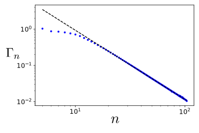
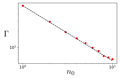
Figure 1: Dots on the left panel represent values of $\Gamma_{n}$ when $n_{0}=4$ and $\alpha=\frac{\pi}{2}$, while the dashed line is the best-fit power law function. Dots on the right panel represent radiation efficiency $\Gamma$ dependence on $n_{0}$ when $\alpha=\frac{\pi}{2}$, while the dashed line shows the function $\Gamma\propto\frac{1}{n_{0}}$.

To understand how the efficiency of radiation $\Gamma$ depends on the loop length $\ell$, we need to perform the infinite sum in (4.12). To do so, we follow the approach described in [26], namely, we calculate and sum numerically the first $100$ values of $\Gamma_{n}$ and approximate the rest of the sum by a power law function that appears as the best fit illustrated on the left panel of figure 1. In that way, we obtain the full radiation efficiency $\Gamma$ for different values of $n_{0}$, shown on the right panel of figure 1. The best-fit value for the case of $\alpha=\frac{\pi}{2}$ is given by $\Gamma(\ell)=\Gamma_{0}\ell^{-0.985\pm 0.001}$, where $\Gamma_{0}=(57\pm 8)\frac{M}{4\pi}$ and does not depend on the string loop length. Thus, rounding the value, one obtains that the string loop decays according to

$$\frac{d\ell(\tau)}{d\tau}\approx-\Gamma_{0}/\ell(\tau)\quad\rightarrow\quad\ell(\tau)^{2}=\ell(0)^{2}-\Gamma_{0}\tau,$$ (4.14)

which means that the lifetime of the cuspless Abelian-Higgs loop is given by $\tau^{*}=\ell^{2}/\Gamma_{0}$, i.e. the same proportionality obtained by the field-theory simulations in refs. [51, 52].

We must emphasize that the number of kinks on loops changes the value of $\Gamma_{0}$, but the proportionality $\tau^{*}\propto\ell^{2}$ remains the same. However, we anticipate that for more generic shapes of loops, the relation between the lifetime $\tau^{*}$ and length $\ell$ of the loop will be different, which was demonstrated in simulations for loops extracted directly from the string network evolution [52]. Decay of other types of loops caused by massive radiation, and detailed comparison with field-theory simulations we leave for future investigation.

5 Conclusion and future work

In this study we investigated Abelian-Higgs cosmic string model. Through the use of duality transformations, we established that the Nambu-Goto action coupled with the massive Kalb-Ramond field provides an effective description of infinitely thin Abelian-Higgs cosmic strings.

By employing Green functions for the massive Kalb-Ramond field, we derived an expression for the classically renormalized tension of Abelian-Higgs cosmic strings. Notably, unlike in the global case, the renormalized tension of local cosmic strings exhibits variations along the worldsheet, with maximum values occurring at kinks and cusps. This maximal value is identical to the one that global cosmic strings have.

Furthermore, we obtained integral expressions for the back-reaction effect of Abelian-Higgs cosmic strings. For the same reason as for particles [68], local equations of motion with analogue of Abraham-Lorentz-Dirac force are not viable. Instead, the full integro-differential expression must be employed to account for the back-reaction effect. It would be interesting to compare these results with field-theory simulations to gain further insights [31, 76].

We also studied the massive radiation for Abelian-Higgs strings. We demonstrated that for a periodically oscillating loop the radiated energy flux per solid angle is given by eq. (4.9). This expression depends on a loop length $\ell$, in contrast to global cosmic strings. We applied the obtained equation for a cuspless type of loop and demonstrated that radiation efficiency $\Gamma$ for cuspless Abelian-Higgs loops exhibits a linear decrease as the loop size increases. Consequently, the decay of the cosmic string loop suggests that the lifetime is proportional to the square of the loop length: $\tau^{*}\propto\ell^{2}$. This finding aligns with the relation obtained in numerical simulations [51, 52].

The outcomes of our research hold significant implications for understanding the back-reaction and radiation processes associated with Abelian-Higgs cosmic strings. They shed light on the discrepancies between field theory and Nambu-Goto simulations. By presenting these findings, we aim to contribute to the ongoing exploration of Abelian-Higgs cosmic strings [51, 52, 31]. Our results open up avenues for further investigation and provide valuable insights into the behavior of these cosmic structures.

References

- [1] D. Tong, TASI lectures on solitons: Instantons, monopoles, vortices and kinks, in proceedings of the Theoretical Advanced Study Institute in Elementary Particle Physics: Many Dimensions of String Theory (TASI 2005), Boulder, Colorado, U.S.A., 5 June–1 July 2005 [arXiv:hep-th/0509216].
- [2] T. Dauxois and M. Peyrard, Physics of solitons, Cambridge University Press (2006), p. 436.
- [3] Y.M. Shnir, Topological and non-topological solitons in scalar field theories, Cambridge University Press (2018), p. 266.
- [4] A. Vilenkin and E.P.S. Shellard, Cosmic strings and other topological defects, Cambridge University Press (2000), p. 517.
- [5] M.B. Hindmarsh and T.W.B. Kibble, Cosmic strings, Rep. Prog. Phys. 58 (1995) 477 [arXiv:hep-ph/9411342].
- [6] R. Jeannerot, J. Rocher and M. Sakellariadou, How generic is cosmic string formation in supersymmetric grand unified theories, Phys. Rev. D 68 (2003) 103514 [arXiv:hep-ph/0308134].
- [7] E.J. Copeland and T.W.B. Kibble, Cosmic strings and superstrings, Proc. R. Soc. A 466 (2010) 623 [arXiv:0911.1345].
- [8] G. Vincent, N.D. Antunes and M. Hindmarsh, Numerical simulations of string networks in the Abelian-Higgs model Phys. Rev. Lett. 80 (1998) 2277 [arXiv:hep-ph/9708427].
- [9] J.N. Moore, E.P.S. Shellard and C.J.A.P. Martins, Evolution of Abelian-Higgs string networks Phys. Rev. D 65 (2001) 023503 [arXiv:hep-ph/0107171].
- [10] M. Hindmarsh, J. Lizarraga, J. Urrestilla, D. Daverio and M. Kunz, Scaling from gauge and scalar radiation in Abelian-Higgs string networks, Phys. Rev. D 96 (2017) 023525 [arXiv:1703.06696].
- [11] J.R.C.C.C. Correia and C.J.A.P. Martins, Abelian–Higgs cosmic string evolution with multiple GPUs, Astron. Comput 34 (2021) 100438 [arXiv:2005.14454].
- [12] J.R.C.C.C. Correia and C.J.A.P. Martins, High resolution calibration of the cosmic strings velocity dependent one-scale model, Phys. Rev. D 104 (2021) 063511 [arXiv:2108.07513].
- [13] A. Drew and E.P.S. Shellard, Radiation from global topological strings using adaptive mesh refinement: methodology and massless modes, Phys. Rev. D 105 (2022) 063517 [arXiv:1910.01718].
- [14] A.-N. Davis, P. Peter, Cosmic strings are current-carrying, Phys. Lett. B 358 (1995) 197 [arXiv:hep-ph/9506433v1].
- [15] Y. Abe, Y. Hamada, K. Yoshioka, Electroweak axion string and superconductivity, JHEP 2021 06 (2021) 172 [arXiv:2010.02834].
- [16] E.J. Copeland, R.C. Myers and J. Polchinski, Cosmic F-and D-strings, JHEP 06 (2004) 013 [arXiv:hep-th/0312067].
- [17] M. Yamada and K. Yonekura, Cosmic F-and D-strings from pure Yang–Mills theory, Phys. Lett. B 838 (2023) 137724 [arXiv:2204.13125].
- [18] I.Y. Rybak, A. Avgoustidis and C.J.A.P. Martins, Dynamics of junctions and the multitension velocity-dependent one-scale model, Phys. Rev. D 99 (2019) 063516 [arXiv:1812.04584].
- [19] I.Y. Rybak, Revisiting Y junctions for strings with currents: Transonic elastic case, Phys. Rev. D 102 (2020) 083516 [arXiv:2001.07262].
- [20] J.R.C.C.C. Correia and C.J.A.P. Martins, Multitension strings in high-resolution U(1)×U(1) simulations, Phys. Rev. D 106 (2022) 043521 [arXiv:2208.01525].
- [21] I.Y. Rybak, C.J.A.P. Martins, P. Peter and E.P.S. Shellard, Cosmological evolution of Witten superconducting string networks, (2023) [arXiv:2304.00053].
- [22] L. Sousa, and P.P. Avelino, Probing cosmic superstrings with gravitational waves, Phys. Rev. D 94 (2016) 063529 [arXiv:1606.05585].
- [23] I.Y. Rybak, A. Avgoustidis and C.J.A.P. Martins, Semianalytic calculation of cosmic microwave background anisotropies from wiggly and superconducting cosmic strings, Phys. Rev. D 96 (10) (2017) 103535 [Erratum ibid 100 (2019) 049901] [arXiv:1709.01839].
- [24] P. Auclair, P. Peter, C. Ringeval and D. Steer, Irreducible cosmic production of relic vortons, JCAP 03 (2021) 098 [arXiv:2010.04620].
- [25] P. Auclair, S. Blasi, V. Brdar and K. Schmitz, Gravitational waves from current-carrying cosmic strings, JCAP 04 (2023) 009 [arXiv:2207.03510].
- [26] I.Y. Rybak and L. Sousa, Emission of gravitational waves by superconducting cosmic strings, JCAP 11 (2022) 024 [arXiv:2209.01068].
- [27] V. Vanchurin, K. Olum, K. and A. Vilenkin, Cosmic string scaling in flat space, Phys. Rev. D 72 (2005) 063514 [arXiv:gr-qc/0501040].
- [28] C.J.A.P. Martins and E.P.S. Shellard, Fractal properties and small-scale structure of cosmic string networks, Phys. Rev. D 73 (2006) 043515 [arXiv:astro-ph/0511792].
- [29] C. Ringeval, M. Sakellariadou and F.R. Bouchet, Cosmological evolution of cosmic string loops, JCAP 02 (2007) 023 [arXiv:astro-ph/0511646].
- [30] J.J. Blanco-Pillado, K.D. Olum and B. Shlaer, Large parallel cosmic string simulations: New results on loop production Phys. Rev. D 83 (2011) 083514 [arXiv:1101.5173].
- [31] J.J. Blanco-Pillado, D. Jiménez-Aguilar, J. Lizarraga, A. Lopez-Eiguren, K.D. Olum, A. Urio and J. Urrestilla, Nambu-Goto Dynamics of Field Theory Cosmic String Loops 2023 [arXiv:2302.03717].
- [32] A. Vilenkin, Cosmic strings as gravitational lenses, Astrophys. J 282 (1984) L51.
- [33] M. Sazhin, M. Khlopov, Cosmic strings and gravitational lens effects, Sov. Astron. 33 (1989) 98.
- [34] O.S. Sazhina, D. Scognamiglio and M.V. Sazhin, Observational constraints on the types of cosmic strings, Eur. Phys. J. C 74 (2014) 1-10 [arXiv:1312.6106].
- [35] A. Lazanu, E.P.S. Shellard and M. Landriau, CMB power spectrum of Nambu-Goto cosmic strings, Phys. Rev. D 91 (2015) 083519 [arXiv:1410.4860].
- [36] A. Lazanu and E.P.S. Shellard, Constraints on the Nambu-Goto cosmic string contribution to the CMB power spectrum in light of new temperature and polarisation data, JCAP 02 (2015) 024 [arXiv:1410.5046].
- [37] J. Lizarraga, J. Urrestilla, D. Daverio, M. Hindmarsh and M. Kunz, New CMB constraints for Abelian Higgs cosmic strings, JCAP 10 (2016) 042 [arXiv:1609.03386].
- [38] T. Charnock, A. Avgoustidis, E.J. Copeland and A. Moss, CMB constraints on cosmic strings and superstrings, Phys. Rev. D 93 (2016) 123503 [arXiv:1603.01275].
- [39] I.Y. Rybak and L. Sousa, CMB anisotropies generated by cosmic string loops, Phys. Rev. D 104 (2021) 023507 [arXiv:2104.08375].
- [40] R.P. Silva, L. Sousa and I.Y. Rybak, Cosmic Microwave Background anisotropies generated by cosmic strings with small-scale structure, (2023) [arXiv:2303.07548].
- [41] L. Sousa and P.P. Avelino, Stochastic gravitational wave background generated by cosmic string networks: Velocity-dependent one-scale model versus scale-invariant evolution, Phys. Rev. D 88 (2013) 023516 [arXiv:1304.2445].
- [42] J.J. Blanco-Pillado and K.D. Olum, Stochastic gravitational wave background from smoothed cosmic string loops, Phys. Rev. D 96 (2017) 104046 [arXiv:1709.02693].
- [43] P. Auclair et al., Probing the gravitational wave background from cosmic strings with LISA, JCAP 04 (2020) 034 [arXiv:1909.00819].
- [44] D.C.N. da Cunha, C. Ringeval and F.R. Bouchet, Stochastic gravitational waves from long cosmic strings JCAP 09 (2022) 078 [arXiv:2205.04349].
- [45] M. Hindmarsh and J.Y. Kume, Multi-messenger constraints on Abelian-Higgs cosmic string networks, JCAP 04 (2023) 045 [arXiv:2210.06178].
- [46] R.A. Battye, B. Garbrecht, A. Moss and H. Stoica, Constraints on brane inflation and cosmic strings, JCAP 01 (2008) 020 [arXiv:0710.1541].
- [47] R.A. Battye, B. Garbrecht and A. Moss, Tight constraints on F-and D-term hybrid inflation scenarios, Phys. Rev. D 81 (2010) 123512 [arXiv:1001.0769].
- [48] Y. Cui, M. Lewicki, D.E. Morrissey and J.D. Wells, Cosmic archaeology with gravitational waves from cosmic strings, Phys. Rev. D 97 (2018) 123505 [arXiv:1711.03104].
- [49] J.A. Dror, T. Hiramatsu, K. Kohri, H. Murayama and G. White, Testing the seesaw mechanism and leptogenesis with gravitational waves, Phys. Rev. Lett 124 (2020) 041804 [arXiv:1908.03227].
- [50] M. Yamada and K. Yonekura, Cosmic strings from pure Yang–Mills theory, Phys. Rev. D 106 (2022) 123515 [arXiv:2204.13123].
- [51] D. Matsunami, L. Pogosian, A. Saurabh and T. Vachaspati, Decay of cosmic string loops due to particle radiation, Phys. Rev. Lett 122 (2019) 201301 [arXiv:1903.05102].
- [52] M. Hindmarsh, J. Lizarraga, A. Urio and J. Urrestilla, Loop decay in Abelian-Higgs string networks Phys. Rev. D 104 (2021) 043519 [arXiv:2103.16248].
- [53] R.L. Davis, E.P.S. Shellard, Antisymmetric Tensors and Spontaneous Symmetry Breaking, Phys. Lett. B 214 (1988) 219.
- [54] A. Vilenkin, T. Vachaspati, Radiation of Goldstone Bosons From Cosmic Strings, Phys. Rev. D 35 (1987) 1138.
- [55] Kibble, T.W., Topology of cosmic domains and strings, J. Phys. A 9 (1976) 1387.
- [56] R.A. Battye, E.P.S. Shellard, Global string radiation, Nucl.Phys. B 423 (1994) 260 [arXiv:astro-ph/9311017].
- [57] R.A. Battye, E.P.S. Shellard, String radiative back reaction, Phys. Rev. Lett. 75 (1995) 4354 [arXiv:astro-ph/9408078].
- [58] R.A. Battye, E.P.S. Shellard, Radiative back reaction on global strings Phys. Rev. D 53 (1996) 1811 [arXiv:hep-ph/9508301].
- [59] A. Dabholkar, J.M. Quashnock, Pinning Down the Axion, Nucl.Phys. B 333 (1990) 815.
- [60] M. Dine, F. Nicolas, G. Akshay and H.P. Hiren, Comments on axions, domain walls, and cosmic strings, JCAP 11 (2021) 041 [arXiv:2012.13065].
- [61] E.J. Copeland, D. Haws and M. Hindmarsh, Classical theory of radiating strings, Phys. Rev. D 42 (1990) 726.
- [62] L., Kimyeong, Dual formulation of cosmic strings and vortices, Phys. Rev. D 48 (1993) 2493 [arXiv:hep-th/9301102].
- [63] A. Smailagic, E. Spallucci, The dual phases of massless/massive Kalb-Ramond fields, J. Phys. A 34 (2001) L435 [arXiv:hep-th/0106173].
- [64] F.A.S. Barbosa, Canonical analysis of Kalb–Ramond–Proca duality, Eur. Phys. J. Plus 137 (2022) 678 [arXiv:2203.08867].
- [65] I. L. Buchbinder, E. N. Kirillova, and N. G. Pletnev, Quantum Equivalence of Massive Antisymmetric Tensor Field Models in Curved Space, Phys. Rev. D 78 (2008) 084024 [arXiv:0806.3505].
- [66] A.Aurilia, Y.Takahashi, Generalized Maxwell Equations and the Gauge Mixing Mechanism of Mass Generation, Progr. Theor. Phys. 66 (1981) 693.
- [67] A.O. Barut, Electrodynamics and classical theory of fields and particles, New York, USA: Dover (1980) p. 235.
- [68] S. Iso, S. Zhang, Radiation Reaction by Massive Particles and Its Non-Analytic Behavior, Phys. Rev. D 86 (2012) 125019 [arXiv:1207.7216].
- [69] P.A.M. Dirac, Classical theory of radiating electrons, Proc. R. Soc. Lond. 167 (1938) 148.
- [70] F. Lund and T. Regge, Unified approach to strings and vortices with soliton solutions, Phys. Rev. D 14 (1976) 1524.
- [71] I. S. Gradshteyn and I. M. Ryzhik, Table of Integrals, Series, and Products, Academic Press, (2007) p.1172.
- [72] M. Li and R. Ruffini, Radiation of new particles of the fifth interaction, Phys. Lett. A 116 (1986) 20.
- [73] P.V. Nieuwenhuizen, Radiation of massive gravitation, Phys. Rev. D 7 (1973) 2300.
- [74] D.E. Krause, H.T. Kloor and E. Fischbach, Multipole radiation from massive fields: Application to binary pulsar systems, Phys. Rev. D 49 (1994) 6892.
- [75] D. Garfinkle, T. Vachaspati, Fields due to kinky, cuspless, cosmic loops, Phys. Rev. D 37 (1988) 257.
- [76] A. Drew and E.P.S. Shellard, Radiation from global topological strings using adaptive mesh refinement: Massive modes, Phys. Rev. D 107 (2023) 043507 [arXiv:2211.10184].