Group velocity and energy propagation in a dielectric medium
supporting magnetic current

Abstract

The aspects of the group velocity and the electromagnetic energy transport for a dielectric medium endowed with magnetic conductivity are discussed. The dispersion relations and the correspondent optical effects are examined for isotropic and anisotropic magnetic conductivity tensors. The group and energy velocities are presented and carried out for all the particular cases addressed. Our results state that a dielectric supporting magnetic current breaks the usual equivalence between group velocity and energy velocity that holds in a non-absorbing medium, while establish the equivalence between them in an effective absorbing scenario, two unexpected behaviors.

I Introduction

A magnetic linear current law, as ${\bf J}={\sigma}_{B}{\bf B}$, appears in some systems due to an asymmetry between the number density of left- and right-handed chiral fermions as a macroscopic manifestation of the quantum Chiral Magnetic Effect (CME) [1]. Such an effect has been much investigated in physics actually, passing in several distinct scenarios, such as quark-gluon plasmas with a chiral chemical potential under the influence of an external magnetic field [2, 3], cosmic magnetic fields in the early Universe [4, 5], Cosmology [6], neutron stars [7, 8], electroweak interactions [11, 12]. In condensed-matter systems, the CME is connected with the physics of Weyl semimetals [13], where the massless fermions acquire a drift velocity along the magnetic field, whose direction is given by their chirality. Opposite chirality implies opposite velocities, creating a chiral-fermion imbalance that is proportional to the chiral magnetic current. Weyl semimetals and CME were examined in the absence of Weyl nodes [15], anisotropic effects stemming from tilted Weyl cones [16], the CME and anomalous transport in Weyl semimetals [17], quantum oscillations arising from the CME [18], computation of the electromagnetic fields produced by an electric charge near a topological Weyl semimetal with two Weyl nodes [19], and the chiral superconductivity [20].

The parity-odd Maxwell-Carroll-Field-Jackiw model (MCFJ) [21] is a Lorentz-violating electrodynamics characterized by the term,

$$\mathrm{{\mathcal{L}_{CFJ}}}=-\frac{1}{4}\epsilon^{\mu\nu\alpha\beta}\left(k_{AF}\right)_{\mu}A_{\nu}F_{\alpha\beta},$$ (1)

where $\left(k_{AF}\right)_{\mu}$ is the 4-vector background which violates Lorentz symmetry. This CPT-odd U(1) model is a piece of the Standard Model Extension (SME) [22], proposed to examine and to constrain the possibility of Lorentz violation in nature. The MCFJ model is a proper theoretical framework to address the CME in an effective classical way [23] since it provides a modified Ampère’s law including the magnetic current, $\mathbf{J}_{B}=k_{AF}^{0}\mathbf{B}$, where the zero component $k_{AF}^{0}$ works as the magnetic conductivity. The MCFJ model is also a possible version of the axion coupling [24], $\theta(\mathbf{E}\cdot\mathbf{B)}$, when the axion field presents constant derivative, $\left(k_{AF}\right)_{\mu}=\partial_{\mu}\theta$. Axion theories constitute a relevant topical research area actually [25, 26, 27, 28]. A classical description of wave propagation, refractive indices, and optical effects, in the context of a matter medium governed by the MCFJ electrodynamics, was discussed in Ref. [29], which also addresses higher-order derivative terms. The MCFJ electrodynamics was much examined, including studies with radioactive corrections [30], topological defects solutions [31], supersymmetric generalizations [32], classical solutions, quantum aspects and unitarity analysis [33]. Lorentz-violation in continuous media  [34, 35] has been a focus of attention in the latest years due to its potential to describe interesting effects of the phenomenology of new materials, such as Weyl semimetals [36].

In a recent work [37], it was examined the classical wave propagation in a conventional dielectric medium, $\mathbf{D}={\epsilon}\,\mathbf{E}$, $\mathbf{B}={\mu}\,\mathbf{H}$, in the presence of a magnetic density current, $J^{i}=\sigma^{B}_{ij}B^{j}$, in which $\sigma^{B}_{ij}$ is the magnetic conductivity. This study was first performed for the case of an isotropic current, which describes the CME observed in Weyl semimetals, $J_{\mathrm{CME}}^{i}={\sigma}^{B}\,B^{i}$, with the attainment of the refractive indices and electric fields for the propagating modes. Configurations with the anisotropic conductivity tensor were also investigated, with some interesting results and repercussions in the literature  [38].

As well known, the electromagnetic energy balance in a continuous medium is stated by the Poynting’s theorem [39, 40, 41],

$$\nabla\cdot{\bf S}+\frac{\partial u_{EM}}{\partial t}=-\,{\bf J}\cdot{\bf E}\;,$$ (2)

in which the Poynting vector is defined by

$${\bf S}=\frac{1}{2}\left({\bf E}\times{\bf H}^{\ast}\right)\;,$$ (3)

and $u_{EM}$ represents the electromagnetic energy density stored in the field. For an isotropic dispersive media such an energy density is given by [40, 39]

$$u_{EM} =\frac{1}{2}\frac{\partial[\omega\epsilon^{\prime}]}{\partial\omega}\left({\bf{E}}\cdot{\bf{E}}^{*}\right)+\frac{1}{2}\frac{\partial[\omega\mu^{\prime}]}{\partial\omega}\left({\bf{H}}\cdot{\bf{H}}^{*}\right)\;,$$ (4)

where $\epsilon^{\prime}$ and $\mu^{\prime}$ are the real pieces of the permittivity and permeability, i.e.,

$$\epsilon(\omega)=\epsilon^{\prime}(\omega)+i\epsilon^{\prime\prime}(\omega),\quad\mu(\omega)=\mu^{\prime}(\omega)+i\mu^{\prime\prime}(\omega)\;,$$ (5)

also endowed with imaginary pieces, $\epsilon^{\prime\prime}(\omega)$, $\mu^{\prime\prime}(\omega)$, in the general situations. For an electric dispersive medium ruled by the isotropic constitutive relations,

$${\bf{D}} =\epsilon(\omega)\,{\bf{E}}\;,\quad{\bf{H}}=\mu^{-1}\,{\bf{B}}\,,$$ (6)

whose Poynting vector and energy density are

$${\bf S}\! = \!\frac{1}{2\mu^{\prime}}\left({\bf E}\times{\bf B}^{\ast}\right)\;,$$ (7a)

$$u_{EM}\! = \!\frac{1}{2}\frac{\partial[\omega\epsilon^{\prime}]}{\partial\omega}\left({\bf{E}}\cdot{\bf{E}}^{*}\right)+\frac{1}{2\mu^{\prime}}\left({\bf{B}}\cdot{\bf{B}}^{*}\right)\;.$$ (7b)

Considering a plane-wave ansatz for the fields,

$$\mathbf{(E,D)}=(\mathbf{E}_{0},\mathbf{D}_{0})\,e^{\mathrm{i}(\mathbf{k}\cdot\mathbf{r}-\omega t)}\;,$$ (8a)

$$\mathbf{(B,H)}=(\mathbf{B}_{0},\mathbf{H}_{0})\,e^{\mathrm{i}(\mathbf{k}\cdot\mathbf{r}-\omega t)}\;,$$ (8b)

where $\omega$ is the harmonic frequency, and the ${\bf k}$ is the wave vector. The Faraday law reads $\omega\,{\bf B}={\bf k}\times{\bf E}$. For the case in which the wave vector and electric field are complex,

$${\bf k}={\bf k}^{\prime}+i\,{\bf k}^{\prime\prime},\quad{\bf E}={\bf E}^{\prime}+i\,{\bf E}^{\prime\prime}\;,$$ (9)

the Poynting vector is given by

$${\bf{S}} =\frac{1}{2\mu^{\prime}\omega}\left[|{\bf{E}}|^{2}{\bf{k}}^{*}-\left({\bf{E}}\cdot{\bf{k}}^{*}\right){\bf{E}}^{*}\right]\;.$$ (10)

In the absence of charges, with $\rho=0$, the isotropic constitutive relation (6) assures the existence of the transversal modes, ${\bf{k}}^{\prime}\cdot{\bf{E}}={\bf{k}}^{\prime\prime}\cdot{\bf{E}}=0$. Under these conditions, the time average for the Poynting vector and for the EM energy density are

$$\left\langle{\bf{S}}\right\rangle\! = \!\frac{{\bf{E}}^{2}}{2\mu^{\prime}}\,{\bf k}^{\prime}\;,$$ (11a)

$$\left\langle u_{EM}\right\rangle\! = \!\frac{1}{4}\left[\epsilon^{\prime}+\omega\,\frac{\partial\epsilon^{\prime}}{\partial\omega}+\frac{|{\bf{k}}|^{2}}{\mu\omega^{2}}\right]{\bf{E}}^{2}\;.$$ (11b)

In a dispersive and non-absorbing medium ($\epsilon^{\prime\prime}=0$), the electromagnetic signal propagation is governed by the group velocity,

$${\bf{v}}_{g} =\frac{\partial\omega}{\partial k}\;,$$ (12)

which for a dispersive and absorbing medium ($\epsilon^{\prime\prime}\neq 0$) becomes a complex velocity, whose physical interpretation is usually unclear [43, 42]. Hence, in absorbing media, the signal propagation is better ruled by the energy velocity [44, 45, 46, 47], a ratio between the averaged Poynting vector and the averaged energy density,

$${\bf{v}}_{E} =\frac{\left\langle{\bf{S}}\right\rangle}{\left\langle u_{EM}\right\rangle}\;,$$ (13)

which provides

$${\bf{v}}_{E}=\frac{\displaystyle{{\bf{k}}^{\prime}}/{\mu\omega}}{\displaystyle{\epsilon^{\prime}}/{2}+\frac{\omega}{2}\frac{\partial\epsilon^{\prime}}{\partial\omega}+|{\bf{k}}|^{2}/{2\mu\omega^{2}}}\;,$$ (14)

that depends on the permittivity and dispersion relation of the medium. For a non-absorbing medium, the group and energy velocities are equal, ${\bf{v}}_{g}={\bf{v}}_{E}$, while for an absorbing medium, such equality does not hold anymore,

$${\bf{v}}_{g}\neq{\bf{v}}_{E}=\frac{\left\langle{\bf{S}}\right\rangle}{\left\langle u_{EM}\right\rangle}\;.$$ (15)

Connections between group and energy velocities were explored in dissipative dynamical systems in Ref. [48]. Part of this procedure was used here to investigate the signal/energy propagation in a chiral dielectric medium endowed with magnetic conductivity, which is still an opened issue. Such a study is the main topic examined in the present work, which also complements the results attained in Ref. [37]. In this context, we point out that a dielectric medium ($\epsilon^{\prime}\neq 0$, $\epsilon^{\prime\prime}=0$), in the presence of isotropic magnetic conductivity, presents real refractive indices and no absorbing behavior, see Eq. (28). Such a non-absorbing medium, however, possesses group velocity distinct from the energy velocity, an unexpected result stemming from the presence of magnetic conductivity. For an antisymmetric conductivity tensor, the opposite unexpected behavior is reported. Indeed, in this case, the refractive index is complex, there existing absorption, but it holds ${\bf{v}}_{g}={\bf{v}}_{E}$.

This work is outlined as follows: in Sec. II we briefly review basic aspects of chiral electrodynamics in matter, examining some optical effects. In Sec. III we discuss aspects of the energy stored in the electromagnetic field and energy flux by electromagnetic waves. By introducing the chiral magnetic current, $J^{i}=\sigma_{B}^{ij}\,B^{j}$, we study the cases in which the magnetic conductivity tensor $\sigma_{B}^{ij}$ is diagonal (isotropic), antisymmetric and symmetric. We investigate the group velocity and the energy propagation velocity for these particular scenarios. The group velocity and energy velocity are calculated in all these cases. We compare the scenarios of an absorbing and non-absorbing medium with the results of the literature. In Section IV we summarize our results.

II Electrodynamics with a magnetic conductivity and optical effects

In this section, we review some basic aspects of a classical electrodynamics in the presence of a magnetic current density, as previously developed in Ref. [37], also examining the correspondent optical effects. We take as starting point, the Maxwell equations for a linear, homogeneous, and isotropic medium are

$$\nabla\cdot{\bf D}\! = \!\rho,\hskip 8.5359pt\hskip 8.5359pt\nabla\times{\bf E}+\frac{\partial{\bf B}}{\partial t}={\bf 0}\;,$$ (16a)

$$\nabla\cdot{\bf B}\! = \!0,\hskip 8.5359pt\hskip 8.5359pt\nabla\times{\bf H}-\frac{\partial{\bf D}}{\partial t}={\bf J}\;,$$ (16b)

where $\rho$ and ${\bf J}$ are classical sources of charges and currents. Using the constitutive relations (6), the magnetic current ${\bf J}={\sigma}_{B}{\bf B}$, plane-wave solutions ansatz (8a) and (8b), and the Faraday’s law, the Ampere-Maxwell’s law (16b) can be written as

$${\bf{k}}\times{\bf{k}}\times{\bf{E}}+\mu\,\epsilon\,\omega^{2}\,{\bf{E}}+\mathrm{i}\,\mu\,\sigma_{B}\,{\bf{k}}\times{\bf{E}}=0\;.$$ (17)

For an anisotropic medium, the magnetic current,

$${J}^{i}={\sigma}_{ij}^{B}\,{B}^{j}\;,$$ (18)

is written in terms of the conductivity tensor, $\sigma^{B}_{ij}$, depends on the material properties. With it, Eq. (19) reads

$$({\bf{k}}\times{\bf{k}}\times{\bf{E}})_{i}+\mu\,\epsilon\,\omega^{2}\,{{E}_{i}}+\mathrm{i}\,\mu\,{\sigma}_{ij}^{B}({\bf{k}}\times{\bf{E}})_{j}=0\,.$$ (19)

The wave equation for the electric field amplitude is

$$\left[\,{\bf k}^{2}\,\delta_{ij}-k_{i}\,k_{j}-\omega^{2}\mu\,\overline{\epsilon}_{ij}(\omega)\,\right]E_{j}=0\;,$$ (20)

where we have defined the permittivity tensor

$$\overline{\epsilon}_{ij}(\omega)=\epsilon(\omega)\,\delta_{ij}-\frac{i}{\omega^{2}}\,\sigma^{B}_{ia}\,\epsilon_{abj}\,k_{b}\;.$$ (21)

The eq. (20) is also written as ${M}_{ij}E^{j}=0$, with

$${M}_{ij}={\bf k}^{2}\,\delta_{ij}-k_{i}\,k_{j}-\omega^{2}\mu\,\overline{\epsilon}_{ij}(\omega)\;.$$ (22)

The non-trivial solutions require that the determinant is null

$$\det[{M_{ij}}]=0\;,$$ (23)

which provides the dispersion relations of the model. In the next sections, we consider materials whose constitutive relations are given by Eq. (6) and endowed with the magnetic conductivity (18) parameterized through isotropic, symmetric and antisymmetric configurations for the magnetic conductivity tensor $\sigma^{B}_{ij}$ .

II.1 Isotropic diagonal chiral conductivity

As a first situation, we review the case of an isotropic magnetic conductivity, that is, $\sigma^{B}_{ij}=\Sigma\,\delta_{ij}$, where $\Sigma$ is a real parameter, which replaced in Eq. (21), yields

$${\bar{\epsilon}}_{ij}(\omega)=\epsilon\,{\delta}_{ij}-{\frac{{\mathrm{i}\Sigma}}{{\omega}^{2}}}\,\epsilon_{ijb}\,k_{b}\,.$$ (24)

For this case, the matrix $M_{ij}$ (22), using ${\bf{n}}={\bf{k}}/\omega$, reads

$$[M_{ij}]=\mathcal{N}+\left(\begin{array}[]{ccc}0&\mathrm{i}\mu n_{3}\frac{\Sigma}{\omega}&-\mathrm{i}\mu n_{2}\frac{\Sigma}{\omega}\\ \\ -\mathrm{i}\mu\frac{n_{3}\Sigma}{\omega}&0&\mathrm{i}\mu n_{1}\frac{\Sigma}{\omega}\\ \\ \mathrm{i}\mu n_{2}\frac{\Sigma}{\omega}&-\mathrm{i}\mu n_{1}\frac{\Sigma}{\omega}&0\end{array}\right),$$ (25)

where

$$\mathcal{N}=\begin{pmatrix}n_{2}^{2}+n_{3}^{2}-\mu\epsilon&-n_{1}n_{2}&-n_{1}n_{3}\\ -n_{1}n_{2}&n_{1}^{2}+n_{3}^{2}-\mu\epsilon&-n_{2}n_{3}\\ -n_{1}n_{3}&-n_{2}n_{3}&n_{1}^{2}+n_{2}^{2}-\mu\epsilon\\ \end{pmatrix}\,.$$ (26)

Requiring the null determinant, we obtain

$$n_{\pm}^{2}=\mu\epsilon+2\left(\frac{\mu\Sigma}{2\omega}\right)^{2}\pm\frac{\mu\Sigma}{\omega}\,\sqrt{\mu\epsilon+\left(\frac{\mu\Sigma}{2\omega}\right)^{2}}\;,$$ (27)

so that the refractive indices are

$$n_{\pm} = \sqrt{\mu\epsilon+\left(\frac{\mu\Sigma}{2\omega}\right)^{2}}\pm\frac{\mu\Sigma}{2\omega}\;,$$ (28a)

$$\tilde{n}_{\pm} = -\sqrt{\mu\epsilon+\left(\frac{\mu\Sigma}{2\omega}\right)^{2}}\pm\frac{\mu\Sigma}{2\omega}\;,$$ (28b)

corresponding to four distinct real refractive indices. The two positive ones, $n_{\pm}$, were already examined in Ref. [37] and define a dispersive non-absorbing medium compatible with the birefringence. We also note that there is no absorption (the indices are real), so the chiral conductivity does not imply a conducting behavior for the dielectric medium. The conducting behavior is assured only when it is defined simultaneously with the Ohmic conductivity $(\sigma\neq 0,\sigma^{B}\neq 0)$. The propagation modes for the indices (28a), obtained from the relation $M_{ij}E_{j}=0$ [37], are

$$\mathbf{E}_{\pm}=\frac{1}{n\sqrt{2(n_{1}^{2}+n_{3}^{2})}}\begin{pmatrix}nn_{3}\mp\mathrm{i}n_{1}n_{2}\\ \pm\mathrm{i}(n_{1}^{2}+n_{3}^{2})\\ \mp\mathrm{i}n_{2}n_{3}-nn_{1}\\ \end{pmatrix}\;.$$ (29)

We can write the modes for some propagation directions. As an initial case, we take a wave propagating at the ${\cal Z}$-axis, $\mathbf{n}=(0,0,n_{3})$, for which Eq. (29) yields

$$\mathbf{E}_{\pm}=\frac{1}{\sqrt{2}}\begin{pmatrix}1\\ \pm\mathrm{i}\\ 0\\ \end{pmatrix}\,.$$ (30)

representing the left-handed ($L$) and right-handed ($R$) polarized electromagnetic waves, corresponding to $\mathbf{E}_{+}$ and $\mathbf{E}_{-}$, respectively. As already mentioned, a known consequence of the optical activity of a medium is linear birefringence, occurring when two circularly polarized modes of opposite chiralities, with refractive indices $n_{+}$ and $n_{-}$, respectively, have different phase velocities, $c/n_{+}$ and $c/n_{-}$. This property implies a rotation of the polarization plane of a linearly polarized wave. It is quantified by the specific rotatory power $\delta$, defined as

$$\delta=-\frac{\omega}{2}[\mathrm{Re}(n_{+})-\mathrm{Re}(n_{-})]\;,$$ (31)

which measures the rotation of the oscillation plane of linearly polarized light per unit traversed length in the medium. Here, $n_{+}$ and $n_{-}$ are associated with left and right-handed circularly polarized waves, respectively. For the refractive indices (28a) and (28b), the rotatory power is frequency-independent, depending only on the chiral magnetic conductivity $\Sigma$, namely,

$$\delta=-\frac{\mu\Sigma}{2}\;.$$ (32)

II.2 Nondiagonal antisymmetric conductivity

The magnetic conductivity tensor may be antisymmetric, ${\sigma}_{ij}^{B}=-{\sigma}_{ji}^{B}$, being parametrized as:

$${\sigma}_{ij}^{B}={\epsilon}_{ijk}\,b_{k}\;,$$ (33)

where $b_{k}=(b_{1},b_{2},b_{3})$ is a constant three-vector, and $\epsilon_{ijk}$ is the Levi-Civita symbol. In this case, the permittivity (21) is

$${\bar{\epsilon}}_{ij}(\omega)=\left(\epsilon+\mathrm{i}\,\frac{{\mathbf{k}\cdot\mathbf{b}}}{{\omega}^{2}}\right){\delta}_{ij}-\frac{\mathrm{i}}{{\omega}^{2}}\,k_{i}\,b_{j}\;.$$ (34)

By replacing Eq. (34) in the matrix (22), we obtain :

$$[M_{ij}] =\mathcal{N}+\mathrm{i}\frac{\mu}{\omega}\begin{pmatrix}-(n_{2}b_{2}+n_{3}b_{3})&n_{1}b_{2}&n_{1}b_{3}\\ n_{2}b_{1}&-(n_{1}b_{1}+n_{3}b_{3})&n_{2}b_{3}\\ n_{3}b_{1}&n_{3}b_{2}&-(n_{1}b_{1}+n_{2}b_{2})\\ \end{pmatrix}\;,$$ (35)

where

$$[M]=\begin{pmatrix}n_{2}^{2}+n_{3}^{2}-\mu\epsilon&-n_{1}n_{2}&-n_{1}n_{3}\\ -n_{1}n_{2}&n_{1}^{2}+n_{3}^{2}-\mu\epsilon&-n_{2}n_{3}\\ -n_{1}n_{3}&-n_{2}n_{3}&n_{1}^{2}+n_{2}^{2}-\mu\epsilon\\ \end{pmatrix}\,.$$ (36)

For $\det[M_{ij}]=0$, one obtains a doubly degenerate dispersion equation in $\mathbf{n}$,

$$\left[n^{2}-\mathrm{i}{\frac{\mu}{\omega}}\left(\mathbf{b}\cdot\mathbf{n}\right)-\mu\epsilon\right]^{2}=0\;,$$ (37)

which provides the solution for the refractive index,

$$n_{\pm}=\pm\sqrt{\mu\epsilon-\left(\frac{\mu}{2\omega}b\cos\theta\right)^{2}}+\mathrm{i}\frac{\mu}{2\omega}b\cos\theta\,,$$ (38)

where $\mathbf{b}\cdot\mathbf{n}=b\,n\,\cos\theta$ with $b=|\mathbf{b}|$. For $\mu\epsilon\geq(\mu b\cos\theta/2\omega)^{2}$ and $\mu\epsilon\leq(\mu b\cos\theta/2\omega)^{2}$, the refractive index is complex and a pure imaginary, respectively. The imaginary piece implies an anisotropic and dispersive absorption, ruled by a direction-dependent absorption coefficient, given by ${\tilde{\alpha}}=\mu\,b\,\cos\theta$. The real piece, when negative, corresponds to the negative refraction, that is usual in metamaterials.

The propagation modes are found for $\mathbf{n}$ along the $z$-axis and the vector $\mathbf{b}$ written as

$$\mathbf{n}=(0,0,n)\,,\quad\mathbf{b}=b\left(0,\sin\theta,\cos\theta\right)\equiv(0,b_{2},b_{3})\;,$$ (39)

where $\theta$ is the angle between $\mathbf{n}$ and $\mathbf{b}$. The matrix (35) is

$$[[M_{ij}]=\left(\begin{array}[]{ccc}n^{2}-\mu\epsilon-n\frac{\mathrm{i}\mu}{\omega}b_{3}&0&0\\ 0&n^{2}-\mu\epsilon-n\frac{\mathrm{i}\mu}{\omega}b_{3}&0\\ 0&n\frac{\mathrm{i}\mu}{\omega}b_{2}&-\mu\epsilon\\ \end{array}\right)\;,$$ (40)

with $\mathbf{n\cdot b}=nb_{3}$. For the condition $\mu\epsilon\geq(\mu b_{3}/2\omega)^{2}$, the indices (38) possess a real piece. For the index $n_{+}$, the condition $M_{ij}E_{j}=0$ provides two mutually orthogonal propagation modes

$$\mathbf{E}_{\pm}^{(1)}=\frac{1}{\sqrt{2(1+Q^{2})}}\begin{pmatrix}\pm\sqrt{1+Q^{2}}\\ -1\\ -\mathrm{i}Qe^{\mathrm{i}\alpha}\\ \end{pmatrix}\;,$$ (41)

while the index $n_{-}$ has associated,

$$\mathbf{E}_{\pm}^{(2)}=\frac{1}{\sqrt{2(1+Q^{2})}}\begin{pmatrix}\pm\sqrt{1+Q^{2}}\\ 1\\ \mathrm{i}Qe^{\mathrm{-i}\alpha}\\ \end{pmatrix}\,,$$ (42)

that fulfill the relations $\mathbf{E}_{+}^{(1)*}\cdot\mathbf{E}_{-}^{(1)}=0$, $\mathbf{E}_{+}^{(2)*}\cdot\mathbf{E}_{-}^{(2)}=0$, with $Q=b_{2}N/\epsilon\omega$. Here, we parameterized the complex refractive index as $n=Ne^{\mathrm{i}\alpha}$, with $N=\sqrt{n^{*}n}=\sqrt{\mu\epsilon}$, and

$$\tan\alpha=\frac{\mu b_{3}/2\omega}{\sqrt{\mu\epsilon-\left(\mu/2\omega b_{3}\right)^{2}}}\;.$$ (43)

The fields (41) set orthogonal modes associated with $n_{+}$, while (42) stands for orthogonal modes associated with $n_{-}$. If birefringence originates from two linearly polarized modes having different phase velocities, this property is not suitably characterized in terms of the usual rotatory power given by Eq. (31), since the latter is based on a decomposition of a linearly polarized mode into two circularly polarized ones of different chirality. For the case $b_{2}=0$, the solutions (41) and (42) read

$$\mathbf{E}_{\pm}^{(1)}=\frac{1}{\sqrt{2}}\begin{pmatrix}\pm 1\\ -1\\ 0\end{pmatrix},\quad\mathbf{E}_{\pm}^{(2)}=\frac{1}{\sqrt{2}}\begin{pmatrix}\pm 1\\ 1\\ 0\end{pmatrix}\;.$$ (44)

In this case, the birefringence is measured in terms of the phase shift developed between the propagating modes (see Eq. (8.32) in [49]):

$$\frac{\Delta}{l}=\frac{2\pi}{\lambda_{0}}\left[\,\mathrm{Re}(n_{+})-\mathrm{Re}(n_{-})\,\right]\;,$$ (45)

where $\lambda_{0}$ is the wavelength of the electromagnetic radiation in vacuo, and $l$ is the distance in which the wave travels in the birefringent medium. Considering the refractive indices (38), the phase shift per unit length is

$$\frac{\Delta}{l}=\frac{2\pi}{\lambda_{0}}\,\sqrt{\mu\epsilon-\left(\frac{\mu}{2\omega b_{3}}\right)^{2}}\;,$$ (46)

also written as

$$\frac{\Delta}{l}=\omega\,\sqrt{\mu\epsilon-\left(\frac{\mu}{2\omega b_{3}}\right)^{2}}\;.$$ (47)

As the refractive indices (38) possess an imaginary piece, there is absorption for both modes (in equal magnitude), measured by an absorption coefficient  [40], given by $\gamma=2\omega\,\mathrm{Im}(n)$, that is,

$$\gamma=\mu\,b_{3}\;.$$ (48)

In this case, by definition, there is no dichroism.

II.3 Nondiagonal symmetric conductivity tensor

Now we examine the case in which the magnetic conductivity is given by a traceless symmetric tensor, in accordance with the following parametrization:

$$\sigma_{ij}^{B}=\frac{1}{2}\left(a_{i}\,c_{j}+a_{j}\,c_{i}\right)\;,$$ (49)

where $a_{i}$ and $c_{i}$ are the components of two orthogonal background vectors $\mathbf{a}$ and $\mathbf{c}$, i.e., $\mathbf{a}\cdot\mathbf{c}=0$, such that $\sigma_{ii}^{B}=0$. Inserting the Eq. (49) in the permittivity tensor (21) yields

$$\bar{\epsilon}_{ij}=\epsilon\,\delta_{ij}+{\frac{\mathrm{i}}{{2{\omega}^{2}}}}\left(a_{i}\,c_{n}+a_{n}\,c_{i}\right){\epsilon}_{nbj}\,k_{b}\;.$$ (50)

The tensor (22) is explicitly represented by the following matrix:

$$[M_{ij}]=\mathcal{N}-\mathrm{i}\frac{\mu}{2\omega}\begin{pmatrix}\epsilon_{11}&n_{1}(a_{1}c_{3}+a_{3}c_{1})-2n_{3}a_{1}c_{1}&-n_{1}(a_{1}c_{2}+a_{2}c_{1})+2n_{2}a_{1}c_{1}\\ -n_{2}(a_{2}c_{3}+a_{3}c_{2})+2n_{3}a_{2}c_{2}&\epsilon_{22}&n_{2}(a_{2}c_{1}+a_{1}c_{2})-2n_{1}a_{2}c_{2}\\ n_{3}(a_{3}c_{2}+a_{2}c_{3})-2n_{2}a_{3}c_{3}&-n_{3}(a_{3}c_{1}+a_{1}c_{3})+2n_{1}a_{3}c_{3}&\epsilon_{33}\\ \end{pmatrix}\;,$$ (51)

where $\mathcal{N}$ is given by the Eq. (36), and

$$\epsilon_{11} =(a_{1}c_{2}+a_{2}c_{1})n_{3}-(a_{1}c_{3}+a_{3}c_{1})n_{2}\,,$$ (52a)

$$\epsilon_{22} =(a_{2}c_{3}+a_{3}c_{2})n_{1}-(a_{1}c_{2}+a_{2}c_{1})n_{3}\,,$$ (52b)

$$\epsilon_{33} =(a_{3}c_{1}+a_{1}c_{3})n_{2}-(a_{3}c_{2}+a_{2}c_{3})n_{1}\,.$$ (52c)

The evaluation of $\det[M_{ij}]=0$ yields the forthcoming dispersion equation:

$$\left[n^{2}-\mu\epsilon+\mathrm{i}\frac{\mu}{2\omega}\mathbf{n}\cdot(\mathbf{a}\times\mathbf{c})\right]\times$$

$$\times\left[n^{2}-\mu\epsilon-\mathrm{i}\frac{\mu}{2\omega}\mathbf{n}\cdot(\mathbf{a}\times\mathbf{c})\right]=0\,.$$ (53)

Using that $\mathbf{n}\cdot(\mathbf{{a}\times{c}})=n|\mathbf{a}||\mathbf{c}|\cos\varphi$, the Eq. (53) yields the solutions

$$n_{\pm}=\sqrt{\mu\epsilon-\left(\frac{\mu}{{4\omega}}|\mathbf{a}||\mathbf{c}|\cos\varphi\right)^{2}}\pm\mathrm{i}\frac{\mu}{{4\omega}}|\mathbf{a}||\mathbf{c}|\cos\varphi\,.$$ (54)

The structure of the two refractive indices present, i.e., the dependence of the refractive index on an angle between $\mathbf{k}$ and a three-vector ($\mathbf{b}$ for the antisymmetric case and $\mathbf{a}\times\mathbf{c}$ for the current scenario).

In order to examine the propagating modes, we set the magnetic conductivity vectors of the symmetric case as ${\bf{a}}=(a_{1},0,a_{3})$, ${\bf{c}}=(0,c_{2},0)$, such that one obtains

$${\bf{a}}\times{\bf{c}}=(-a_{3}c_{2},0,a_{1}c_{2})\;.$$ (55)

For propagation along the ${\cal Z}$-axis, ${\bf{n}}=(0,0,n)$, the matrix $M_{ij}$ (51) is

$$[M_{ij}] =\begin{pmatrix}n^{2}-\mu{\epsilon}-i\frac{\mu}{2\omega}a_{1}c_{2}n&0&0\\ 0&n^{2}-\mu{\epsilon}+i\frac{\mu}{2\omega}a_{1}c_{2}&0\\ -i\frac{\mu}{2\omega}a_{3}c_{2}n&0&-\mu{\epsilon}\end{pmatrix},$$ (56)

where ${\epsilon}$ is the complex electric permittivity. Evaluating $\mathrm{det}[M_{ij}]=0$, one finds the following dispersion relations:

$$n^{2}-\mu{\epsilon}=\pm i\frac{\mu}{2\omega}\,a_{1}\,c_{2}\,n\;,$$ (57)

which is compatible with Eq. (53).

We then write now the electric field polarizations satisfying $M_{ij}E_{j}=0$ associated with $n^{2}_{+}$ and $n^{2}_{-}$, respectively

$$\hat{\bf{E}}_{+}=\frac{1}{\sqrt{1+|A|^{2}}}\begin{pmatrix}1\\ 0\\ -iA\end{pmatrix}\,,\quad\hat{\bf{E}}_{-}=\begin{pmatrix}0\\ 1\\ 0\end{pmatrix}\,,$$ (58)

where $A={a_{3}c_{2}}/{2\omega{\epsilon}n}$. We observe that $\hat{\bf{E}}_{\pm}$ represent the linearly polarized vectors, with $\hat{\bf{E}}_{+}$ endowed with a longitudinal component.

If we consider refractive indices from (53) with the positive real piece, the propagation turns out free of birefringence. However, since the imaginary pieces are different, the propagating modes are absorbed in different degrees, which can be measured by the absorption difference per unit length,

$$\frac{\Delta_{d}}{l}=\frac{2\pi}{\lambda_{0}}\,\left[\,\mathrm{Im}(n_{+})-\mathrm{Im}(n_{-})\,\right]\,,$$ (59)

which for the indices (54) and propagation along the $x$-axis, yields

$$\frac{\Delta_{d}}{l}=\frac{\mu a_{1}\,c_{2}}{2}\;.$$ (60)

III Energy propagation

In this section, we will discuss some aspects regarding the energy velocity and group velocity considering the three scenarios endowed with magnetic conductivity, $\sigma^{B}_{ij}$, already discussed.

III.1 Isotropic magnetic conductivity

Let us begin with the isotropic magnetic conductivity, $\sigma^{B}_{ij}=\Sigma\,\delta_{ij}$, where $\Sigma$ is a real and positive constant, that represents $1/3$ of the trace of the $\sigma^{B}_{ij}$ matrix. Substituting this tensor in Eq. (21), the determinant condition (23) yields the $k$-polynomial equation

$$\left[\,k^{2}-\mu\,\epsilon(\omega)\,\omega^{2}\,\right]^{2}-\mu^{2}\,\Sigma^{2}\,k^{2}=0\;.$$ (61)

Remembering that $\epsilon(\omega)=\epsilon^{\prime}(\omega)+i\epsilon^{\prime\prime}(\omega)$, the solutions of Eq. (61) are

$$k_{\pm} =\omega\left(I_{+}+i\,I_{-}\right)\pm\frac{\mu\Sigma}{2}\;,$$ (62a)

$$\tilde{k}_{\pm} =-\omega\left(I_{+}+i\,I_{-}\right)\pm\frac{\mu\Sigma}{2}\;,$$ (62b)

with

$$I_{\pm} =\frac{\hat{I}_{\pm}}{\sqrt{2}}\sqrt{\mu\epsilon^{\prime}+\left(\frac{\mu\Sigma}{2\omega}\right)^{2}}\;,$$ (62c)

$$\hat{I}_{\pm} =\sqrt{\sqrt{1+\left(\frac{\mu\epsilon^{\prime\prime}}{\mu\epsilon^{\prime}+\mu^{2}\Sigma^{2}/(4\omega^{2})}\right)^{2}}\pm 1}\;.$$ (62d)

Implementing ${\bf{n}}={\bf{k}}/\omega$ in Eq. (62), one obtains the following associated refractive indices:

$$n_{\pm} =\left(I_{+}+i\,I_{-}\right)\pm\frac{\mu\Sigma}{2\omega}\;,$$ (63a)

$$\tilde{n}_{\pm} =-\left(I_{+}+i\,I_{-}\right)\pm\frac{\mu\Sigma}{2\omega}\;,$$ (63b)

where $\tilde{n}_{\pm}$ is associated with negative refraction. The behavior of $n_{\pm}$ as a function of the frequency $\omega$ is plotted in Fig. 1, where for illustration, we have considered $\epsilon^{\prime\prime}=i(\sigma/\omega)$, with $\sigma$ being the Ohmic conductivity. Figure 1 also reveals a kind of mirror symmetry between the refractive indices $\tilde{n}_{\pm}$ and $n_{\pm}$, ascribed to $\tilde{n}_{\pm}=-n_{\mp}$. In the following, we use natural units.

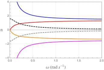
Figure 1: Refractive indices of Eq. (63) in terms of $\omega$. The solid blue (red) line illustrates $\mathrm{Re}[n_{\pm}]$, while the dashed black line depicts $\mathrm{Im}[n_{\pm}]$. The solid orange (magenta) line illustrates $\mathrm{Re}[\tilde{n}_{\pm}]$, while the dashed gray line depicts $\mathrm{Im}[\tilde{n}_{\pm}]$. Here we have used $\mu=1$, $\epsilon^{\prime}=2$, $\sigma=0.8$ $\mathrm{s}^{-1}$, $\Sigma=0.5$ $\mathrm{s}^{-1}$.

In the presence of absorption terms, the group velocity is not a real quantity, no longer representing the energy propagation velocity. As illustration, we take the dispersion relations (62) and derive the group velocity, $v_{g}=~{}(\partial\omega/\partial k)$, associated with it, obtaining the expression

$$v_{g}^{\pm} =\frac{\displaystyle\frac{k^{\prime}_{\pm}}{\mu\omega}\mp\frac{\Sigma}{2\omega}+i\frac{\omega\epsilon^{\prime\prime}}{2k^{\prime}_{\pm}}\left(1\mp\frac{\mu\Sigma}{2k^{\prime}_{\pm}}\right)^{-1}}{\displaystyle\epsilon^{\prime}+\frac{\omega}{2}\frac{\partial\epsilon^{\prime}}{\partial\omega}+i\left(\epsilon^{\prime\prime}+\frac{\omega}{2}\frac{\partial\epsilon^{\prime\prime}}{\partial\omega}\right)},$$ (64)

which is complex, as it usually occurs in an absorbing and active media [48]. In this case, in order to analyze the propagation of energy carried by the wave through the medium, we need to evaluate the energy velocity instead of the group velocity. Such velocity is obtained using Eq. (62a) and Eq. (62b) in Eq. (14), for the propagating modes described by $k_{\pm}$ and $\tilde{k}_{\pm}$, namely:

$$V_{E}^{\pm} =\frac{2\omega I_{+}\pm{\mu\Sigma}}{2\omega U^{I}_{\pm}}\;,\quad\widetilde{V}_{E}^{\pm}=\frac{-2\omega I_{+}\pm\mu\Sigma}{2\omega U^{I}_{\mp}}\;,$$ (65)

with

$$U^{I}_{\pm} =\frac{\mu\epsilon^{\prime}}{2}+\frac{\mu\omega}{2}\frac{\partial\epsilon^{\prime}}{\partial\omega}+\frac{1}{2}(I_{+}^{2}+I_{-}^{2})+\frac{\mu^{2}\Sigma^{2}}{8\omega^{2}}\pm\frac{\mu\Sigma I_{+}}{2\omega}.$$ (66)

Clearly, the energy velocity (65) is different from the group velocity (64), $V_{E}^{\pm}\neq v_{g}^{\pm}$. Such an energy velocity is plotted as a function of the frequency in Fig. 2, with the values of $\mu=1$, $\epsilon^{\prime}=2$, $\sigma=0.8$ $s^{-1}$, and $\Sigma=0.5$ $s^{-1}$. For the high-frequency limit, $\omega\rightarrow\infty$, the energy velocity goes as $v_{E}=\pm\,1/\sqrt{\mu\epsilon}$, with the plus sign holding for the propagating modes associated with $k_{\pm}$, and the minus sign being related to $\tilde{k}_{\pm}$. Notice that when there is no magnetic conductivity ($\Sigma=0)$, the group velocity (64) recovers the same result obtained in Ref. [48].

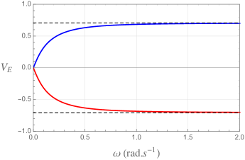
Figure 2: Energy velocity in terms of $\omega$. The solid blue (red) line illustrates $V_{E}^{\pm}$ and $\widetilde{V}_{E}^{\pm}$, while the horizontal dashed black lines depict the asymptotic limits $\pm 1/\sqrt{\mu\epsilon^{\prime}}$. Here we have used $\mu=1$, $\epsilon^{\prime}=2$, $\sigma=0.8$ $\mathrm{s}^{-1}$, $\Sigma=0.5$ $\mathrm{s}^{-1}$.

For non-absorbing dielectrics ($\epsilon^{\prime\prime}=0$), the group and energy velocities are usually equal, $v_{E}=v_{g}$ [48, 44, 40, 47]. Such equality fails, however, in the presence of magnetic conductivity, $\Sigma\neq 0$. Indeed, for $\epsilon^{\prime\prime}=0$, one finds $I_{-}=k_{\pm}^{\prime\prime}=0$, $I_{+}=\sqrt{\mu\epsilon^{\prime}+\mu^{2}\Sigma^{2}/(4\omega^{2})}$, and $k^{\prime}_{\pm}=\omega I_{+}\pm\mu\Sigma/2$, in which the group velocity (64) and the energy velocity (65), respectively, read

$$\left.v_{g}^{\pm}\right|_{\epsilon^{\prime\prime}=0} =\frac{2k^{\prime}_{\pm}\mp\mu\Sigma}{\displaystyle{2\mu\omega}\left(\epsilon^{\prime}+\frac{\omega}{2}\frac{\partial\epsilon^{\prime}}{\partial\omega}\right)}\;,$$ (67a)

$$\left.V_{E}^{\pm}\right|_{\epsilon^{\prime\prime}=0} =\frac{k^{\prime}_{\pm}}{\displaystyle\mu\omega\left(\epsilon^{\prime}+\frac{\omega}{2}\frac{\partial\epsilon^{\prime}}{\partial\omega}\pm\frac{\Sigma}{2\omega^{2}}k_{\pm}^{\prime}\right)}\;,$$ (67b)

constituting distinct expressions, $v_{E}\neq v_{g}$, even when the dielectric substrate is deprived of absorption $(\epsilon^{\prime\prime}=0)$. This is an entire consequence of the isotropic magnetic conductivity, which can not be encoded in the medium permittivity. In fact, note that by setting $\Sigma=0$, Eq. (67a) and Eq. (67b) reduce to the same expression,

$$V_{E}=V_{g}=\frac{k^{\prime}_{\pm}}{\mu\omega\left(\epsilon^{\prime}+\frac{1}{2}\omega({\partial\epsilon^{\prime}/\partial\omega})\right)}\;.$$ (68)

This is a curious result in some respects. In fact, on the one hand, it seems to indicate that the magnetic conductivity implies absorption. On the other hand, equations (28a) and (28b) reveal that the $\Sigma$ conductivity does not engender an imaginary contribution for the refractive indices, holding the absence of absorption (for $\epsilon^{\prime\prime}=0$ and $\Sigma\neq 0$). Therefore, it here appears a novelty: a non-absorptive medium (real refractive index) where the energy velocity and group velocity are unequal. This surprising behavior is due to the presence of the isotropic magnetic current.

III.2 Antisymmetric magnetic conductivity

In this case, the antisymmetric conductivity tensor is parametrized in terms of a constant background vector, ${\bf b}$, as previously mentioned, that is, $\sigma_{ij}^{B}=\epsilon_{ijk}\,b_{k}$. Substituting this antisymmetric tensor in (21), the determinant (23) yields the dispersion relation

$$k^{2}+i\,\mu\,({\bf b}\cdot{\bf k})-\mu\,\epsilon(\omega)\,\omega^{2}=0\;,$$ (69)

whose solutions are

$$k_{\pm}=-\frac{i\,\mu}{2}\,(\hat{{\bf k}}\cdot{\bf b})\pm\sqrt{\mu\,\epsilon(\omega)\,\omega^{2}-\frac{\mu^{2}}{4}(\hat{{\bf k}}\cdot{\bf b})^{2}}\;,$$ (70)

or equivalently,

$$k_{\pm} =-\frac{i\,\mu}{2}\,(\hat{\bf{k}}\cdot{\bf{b}})\pm\omega\left(A_{+}+i\,A_{-}\right)\;,$$ (71a)

with

$$A_{\pm} =\frac{1}{\sqrt{2}}\,\sqrt{\left|f(\omega)\right|\left(\sqrt{1+\frac{\mu^{2}\epsilon^{\prime\prime 2}}{{f(\omega)}^{2}}}\pm\mathrm{sign}[f(\omega)]\right)}\;,$$ (71b)

where

$$f(\omega) =\mu\epsilon^{\prime}-\frac{\mu^{2}(\hat{\bf{k}}\cdot{\bf{b}})^{2}}{4\omega^{2}}\;.$$ (71c)

The refractive indices, $n_{\pm}$, associated with $k_{\pm}$ can be obtained by using ${\bf{n}}={\bf{k}}/\omega$, providing two indices

$$n_{\pm} =-i\,\frac{\mu(\hat{\bf{k}}\cdot{\bf{b}})}{2\omega}\pm(A_{+}+iA_{-})\;,$$ (72)

being $\mathrm{Re}[n_{+}]>0$ and $\mathrm{Re}[n_{-}]<0$ (negative refraction). Using $(\hat{\bf{k}}\cdot{\bf{b}})=b\,\cos\theta$ and $\epsilon(\omega)=\epsilon^{\prime}+i(\sigma/\omega)$, we illustrate the general behavior of the refractive index $n_{\pm}$ in terms of the frequency in Figs. 3 and 4 for the following cases: i) perpendicular ($\theta=\pi/2$), ii) parallel ($\theta=0$), and iii) antiparallel ($\theta=\pi$) configurations. We use $\mu=1$, $\epsilon=2$, $|{\bf b}|=0.3$ $\mathrm{s}^{-1}$, and $\sigma=0.8$ $\mathrm{s}^{-1}$ in these plots. Notice that, when ${\bf b}$ is perpendicular to $\hat{{\bf k}}$-direction, the results do not depend on the magnitude of the ${\bf b}$-vector.

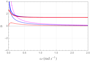
Figure 3: Refractive indice $n_{+}$ of Eq. (72). Solid (dashed) lines represent $\mathrm{Re}[n_{+}]$ ($\mathrm{Im}[n_{+}]$). The particular cases considered are: $\theta=\pi/2$ (blue), $\theta=0$ (red), and $\theta=\pi$ (magenta). Here we have used $\mu=1$, $\epsilon^{\prime}=2$, $\sigma=0.8$ $\mathrm{s}^{-1}$, $b=0.3$ $\mathrm{s}^{-1}$. The solid magenta and red lines lie on top of each other.

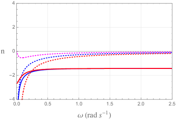
Figure 4: Refractive indice $n_{-}$ of Eq. (72), negative refraction case. Solid (dashed) lines represent $\mathrm{Re}[n_{-}]$ ($\mathrm{Im}[n_{-}]$). The particular cases considered are: $\theta=\pi/2$ (blue), $\theta=0$ (red), and $\theta=\pi$ (magenta). Here we have used $\mu=1$, $\epsilon^{\prime}=2$, $\sigma=0.8$ $\mathrm{s}^{-1}$, $b=0.3$ $\mathrm{s}^{-1}$. The solid magenta and red lines are again superimposed.

We point out that $\mathrm{Re}[n_{\pm}]|_{\theta=0}=\mathrm{Re}[n_{\pm}]|_{\theta=\pi}$, explaining the reason by which the solid magenta and red curves appear superimposed in Figs. 3 and 4. Furthermore, one notices that $\mathrm{Im}[n_{-}]|_{\theta=0}=-\mathrm{Im}[n_{+}]|_{\theta=\pi}$ and $\mathrm{Im}[n_{-}]|_{\theta=\pi}=-\mathrm{Im}[n_{+}]|_{\theta=0}$, which indicates an interchange in the absorptive behavior for $\bf{b}$ parallel and antiparallel configurations. The correspondence $\mathrm{Re}[n_{\pm}]=-\mathrm{Re}[n_{\mp}]$ holds for any propagation configuration. In the high-frequency limit, $n_{\pm}\rightarrow\pm\sqrt{\mu\epsilon^{\prime}}$, which also indicates that the absorption effects reduce drastically in this special limit.

To evaluate the energy velocity associated with $k_{\pm}$, one uses the dispersion relations (71a) in Eq. (14), yielding

$$V_{E}^{\pm} =\frac{\pm A_{+}}{U^{A}_{\pm}}\;,$$ (73)

with

$$U^{A}_{\pm} =\frac{\mu\epsilon^{\prime}}{2}+\frac{\mu\omega}{2}\frac{\partial\epsilon^{\prime}}{\partial\omega}+\frac{1}{2}(A_{+}^{2}+A_{-}^{2})+\frac{\mu^{2}(\hat{\bf{k}}\cdot{\bf{b}})^{2}}{8\omega^{2}}+$$

$$\phantom{=}\mp\frac{\mu(\hat{\bf{k}}\cdot{\bf{b}})A_{-}}{2\omega}\;.$$ (74)

We show the behavior of the energy velocity $V_{E}^{\pm}$ as a function of the frequency in Fig. 5.

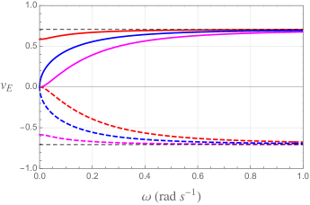
Figure 5: Energy velocity $V_{E}^{\pm}$ of Eq. (73). The particular cases considered are: $\theta=\pi/2$ (blue), $\theta=0$ (red), and $\theta=\pi$ (magenta). Solide lines indicate $V_{E}^{+}$, while the dashed curves represent $V_{E}^{-}$. Here we have used $\mu=1$, $\epsilon^{\prime}=2$, $\sigma=0.8$ $\mathrm{s}^{-1}$, $b=0.3$ $\mathrm{s}^{-1}$.

Taking the differential operation in relation to $k^{i}$-component in (69), the correspondent group velocity is

$${\bf v}_{g}=\frac{\partial\omega}{\partial{\bf k}}=\frac{\displaystyle\frac{{\bf k}}{\mu\omega}+i\,\frac{{\bf b}}{2\omega}}{\displaystyle\left(\epsilon^{\prime}+\frac{\omega}{2}\frac{\partial\epsilon^{\prime}}{\partial\omega}\right)+i\left(\epsilon^{\prime\prime}+\frac{\omega}{2}\frac{\partial\epsilon^{\prime\prime}}{\partial\omega}\right)}\;,$$ (75)

which is valid for all frequency range and for both solutions, $k_{\pm}$. Let us now write the $k^{i}$-components as $k^{i}=k^{\prime i}+i\,k^{\prime\prime i}$, then the group velocity can be rewritten as

$${\bf v}_{g} =\frac{\displaystyle\frac{{\bf k}^{\prime}}{\mu\omega}+i\,\frac{\omega\epsilon^{\prime\prime}\,\hat{{\bf k}}}{2k^{\prime}}}{\displaystyle\left(\epsilon^{\prime}+\frac{\omega}{2}\frac{\partial\epsilon^{\prime}}{\partial\omega}\right)+i\left(\epsilon^{\prime\prime}+\frac{\omega}{2}\frac{\partial\epsilon^{\prime\prime}}{\partial\omega}\right)}\;.$$ (76)

Therefore, the group velocity is in the ${\bf k}$-direction since the contribution of the ${\bf b}$-vector conductivity is canceled.

Differently from the isotropic conductivity case, where the absorption effect occurs only for $\epsilon^{\prime\prime}\neq 0$, in the antisymmetric scenario, the absorption effect can be observed by means of the dispersion relation (69), from which one finds that the absorption occurs for the three subcases:

• $\epsilon^{\prime\prime}=0$ and $b\cos\theta=0$ (absence of absorption);

• $\epsilon^{\prime\prime}=0$ and $b\cos\theta\neq 0$ (magnetically induced absorption effect);

• $\epsilon^{\prime\prime}\neq 0$ and $b\cos\theta\neq 0$ (usual and magnetically induced absorption), for which group and energy velocities are different, as revealed by Eqs. (73) and (76).

In order to analyze the energy velocity and its possible connection with the group velocity, we now consider the two particular cases with potential novelties, that is, the ones with no dielectric absorption, $\epsilon^{\prime\prime}=0$.

For the case (i), $\epsilon^{\prime\prime}=0$ and $b\cos\theta=0$, the complex group velocity of (76) and the energy velocity (73) are equivalent:

$$v_{g}^{\pm}=V_{E}^{\pm}=\frac{{k^{\prime}_{\pm}/\mu\omega}}{\displaystyle\epsilon^{\prime}+\frac{\omega}{2}\frac{\partial\epsilon^{\prime}}{\partial\omega}}\;,$$ (77)

with

$$k^{\prime}_{\pm}=\omega A_{+},\quad k^{\prime\prime}_{\pm}=0,A_{+}=\sqrt{\mu\epsilon^{\prime}},\quad A_{-}=0\;.$$ (78)

This is an expected result, considering the real refractive index, $n=\sqrt{\mu\epsilon^{\prime}}$, that stems from Eq. (38).

For the case (ii), $\epsilon^{\prime\prime}=0$ and $b\cos\theta\neq 0$, the complex group velocity, and the energy velocity are read below

$$v_{g}^{\pm}=V_{E}^{\pm}=\frac{{k^{\prime}_{\pm}/\mu\omega}}{\displaystyle\epsilon^{\prime}+\frac{\omega}{2}\frac{\partial\epsilon^{\prime}}{\partial\omega}}\;,$$ (79)

where, in this case,

$$k^{\prime}_{\pm} =\omega A_{+},\quad k^{\prime\prime}_{\pm}=-\frac{\mu}{2}(\hat{\bf{k}}\cdot{\bf{b}})\pm\omega A_{-}\;,$$ (80a)

$$A_{\pm}=\frac{1}{\sqrt{2}}\sqrt{\left|f(\omega)\right|\left(1\pm\mathrm{sign}[f(\omega)]\right)}\;,$$ (80b)

so that

$$v_{g}^{\pm}=V_{E}^{\pm}=\frac{\sqrt{\left|f(\omega)\right|\left(1+\mathrm{sgn}[f(\omega)]\right)}}{\displaystyle\mu\sqrt{2}\left(\epsilon^{\prime}+\frac{\omega}{2}\frac{\partial\epsilon^{\prime}}{\partial\omega}\right)}\;.$$ (81)

with $f(\omega)$ given by Eq. (71c). Differently from the isotropic conductivity section, the group velocity and energy velocity remain equal even when the anisotropic conductivity is non-null. It is interesting to observe that when $\epsilon^{\prime\prime}=0$ and $b\cos\theta\neq 0$, there is absorption, since the refractive index (38),

$$n_{\pm}=\pm\sqrt{\mu\epsilon^{\prime}-\left(\frac{\mu}{2\omega}b\cos\theta\right)^{2}}+\mathrm{i}\frac{\mu}{2\omega}b\cos\theta\,,$$ (82)

possesses an imaginary piece. Surprisingly, however, the group velocity and energy velocity turn out equivalent in this special absorbing scenario. Therefore, the equality $v_{g}=V_{E}$ holds for the magnetically induced absorption, stemming from the antisymmetric magnetic conductivity tensor.

Here, we need to be careful due to the sign function in Eq. (81), as highlighted below:

• For $f(\omega)>0$, one has $\mathrm{sign}\left[f(\omega)\right]=1$, such that

  $$v_{g}^{\pm}=V_{E}^{\pm}=\frac{\sqrt{\left|f(\omega)\right|}}{\displaystyle\mu\left(\epsilon^{\prime}+\frac{\omega}{2}\frac{\partial\epsilon^{\prime}}{\partial\omega}\right)}\;.$$ (83)

• For $f(\omega)<0$, one has $\mathrm{sign}\left[f(\omega)\right]=-1$, then one finds

  $$v_{g}^{\pm}=V_{E}^{\pm}=0\;,$$ (84)

  which is a consequence of having the wave vector (70) completely imaginary (for this condition).

Such behavior is plotted in Fig. 6, that depicts the energy velocity $V_{E}^{\pm}$ considering $\epsilon^{\prime\prime}=0$ for the parallel and antiparallel configurations. For $0<\omega<\omega^{\prime}$, with

$$\omega^{\prime}=\sqrt{\frac{\mu(\hat{\bf{k}}\cdot{\bf{b}})^{2}}{4\epsilon^{\prime}}}\;,$$ (85)

it holds $f(\omega)<0$ and energy velocity is null, indicating that, in this particular situation, there is no propagation. For $\omega>\omega^{\prime}$, one has $f(\omega)>0$ and the velocities (83).

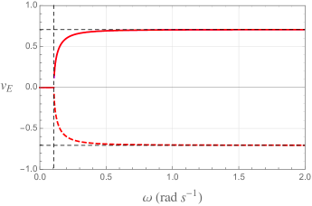
Figure 6: Energy velocity $V_{E}^{\pm}$ of Eq. (73) for $\epsilon^{\prime\prime}=0$. Solide red line indicates $V_{E}^{+}$ for $\theta=(0,\pi)$, while the dashed red curve represents $V_{E}^{-}$ for $\theta=(0,\pi)$. Here we have used $\mu=1$, $\epsilon^{\prime}=2$, $b=0.3$ $\mathrm{s}^{-1}$. The vertical dashed line indicates the frequency $\omega^{\prime}$ of Eq. (85).

III.3 Symmetric magnetic conductivity

The magnetic conductivity tensor in the symmetric form is parametrized by $\sigma^{B}_{ij}=\left(a_{i}\,c_{j}+a_{j}\,c_{i}\right)/2$, where $a_{i}$ and $c_{j}$ are components of the two background vectors ${\bf a}$ and ${\bf c}$, respectively. In this case, the permittivity tensor (21) is

$$\overline{\epsilon}_{ij}(\omega)=\epsilon(\omega)\,\delta_{ij}+\frac{i}{2\omega}\left[\,a_{i}\left({\bf c}\times{\bf n}\right)_{j}+c_{i}\left({\bf a}\times{\bf n}\right)_{j}\,\right]\;.$$ (86)

The null determinant in (23) yields the $k$-polynomial equation

$$k^{2}\pm\frac{i\,\mu}{2}\,({\bf a}\times{\bf c})\cdot{\bf k}\,-\,\mu\,\epsilon(\omega)\,\omega^{2} =0\;,$$ (87)

whose four solutions are

$$k_{\pm} =\pm\frac{i\mu({\bf{a}}\times{\bf{c}})\cdot\hat{\bf{k}}}{4\omega}+\omega(S_{+}+iS_{-})\;,$$ (88a)

$$\tilde{k}_{\pm} =\pm\frac{i\mu({\bf{a}}\times{\bf{c}})\cdot\hat{\bf{k}}}{4\omega}-\omega(S_{+}+iS_{-})\;,$$ (88b)

with

$$S_{\pm} =\frac{1}{\sqrt{2}}\sqrt{|g(\omega)|\left(\sqrt{1+\frac{\mu^{2}\epsilon^{\prime\prime 2}}{g(\omega)^{2}}}\pm\mathrm{sgn}[g(\omega)]\right)}\;,$$ (88c)

$$g(\omega) =\mu\epsilon^{\prime}-\frac{\mu^{2}}{16\omega^{2}}(({\bf{a}}\times{\bf{c}})\cdot\hat{\bf{k}})^{2}\;.$$ (88d)

Using $({\bf{a}}\times{\bf{c}})\cdot\hat{\bf{k}}=|{\bf{a}}\times{\bf{c}}|\cos\varphi$, there appear four refractive indices,

$$n_{\pm} =\pm\frac{i\mu|{\bf{a}}\times{\bf{c}}|}{4\omega}\cos\varphi+(S_{+}+iS_{-})\;,$$ (89a)

$$\tilde{n}_{\pm} =\pm\frac{i\mu|{\bf{a}}\times{\bf{c}}|}{4\omega}\cos\varphi-(S_{+}+iS_{-})\;,$$ (89b)

where $\tilde{n}_{\pm}$ are related with negative refraction.

Figures 7 and 8 illustrate the general behavior of the refractive indices $n_{\pm}$ and $\tilde{n}_{\pm}$ as functions of the frequency for: i) perpendicular ($\varphi=\pi/2$), ii) parallel ($\varphi=0$), and iii) antiparallel ($\varphi=\pi$) configurations.

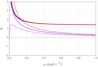
Figure 7: Refractive indice $n_{+}$ of Eq. (89a). Solid (dashed) lines represent $\mathrm{Re}[n_{+}]$ ($\mathrm{Im}[n_{+}]$). The particular cases considered are: $\varphi=\pi/2$ (blue), $\varphi=0$ (red), and $\varphi=\pi$ (magenta). Here we have used $\mu=1$, $\epsilon^{\prime}=2$, $\sigma=0.8$ $\mathrm{s}^{-1}$, $|{\bf{a}}\times{\bf{c}}|=0.3$ $\mathrm{s}^{-1}$. The solid red and magenta curves are coincident, since $\cos^{2}\pi=\cos^{2}0.$

From Eq. (89a), one observes that $\mathrm{Re}[n_{+}]=\mathrm{Re}[n_{-}]$, for all $\varphi$. Also, $\mathrm{Im}[n_{-}]|_{\varphi=\pi}=\mathrm{Im}[n_{+}]|_{\varphi=0}$ and $\mathrm{Im}[n_{-}]|_{\varphi=0}=\mathrm{Im}[n_{+}]|_{\varphi=\pi}$, which indicates that the absorbing terms in $n_{+}$ for the parallel configuration are mapped in absorbing terms in $n_{-}$ for the antiparallel configuration. This kind of analysis allows us to infer the behavior of $n_{-}$ without plotting it.

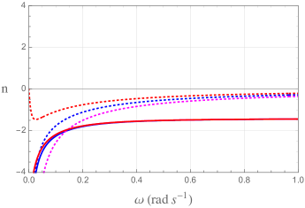
Figure 8: Refractive indice $\tilde{n}_{+}$ of Eq. (89b). Solid (dashed) lines represent $\mathrm{Re}[n_{+}]$ ($\mathrm{Im}[n_{+}]$). The particular cases considered are: $\varphi=\pi/2$ (blue), $\varphi=0$ (red), and $\varphi=\pi$ (magenta). Here we have used $\mu=1$, $\epsilon^{\prime}=2$, $\sigma=0.8$ $\mathrm{s}^{-1}$, $|{\bf{a}}\times{\bf{c}}|=0.3$ $\mathrm{s}^{-1}$. The red and magenta solid curves lie on top of each other, since $\mathrm{Re}[\tilde{n}_{\pm}]|_{\varphi=0}=\mathrm{Re}[\tilde{n}_{\pm}]|_{\varphi=\pi}$.

Comparing the refractive indices $n_{\pm}$ and $\tilde{n}_{\pm}$, one notices that $\mathrm{Re}[\tilde{n}_{\pm}]=-S_{+}=-\mathrm{Re}[n_{\pm}]$. On the other hand,

$$-\mathrm{Im}[\tilde{n}_{\pm}] =S_{-}\mp i\frac{\mu}{4\omega}|{\bf{a}}\times{\bf{c}}|\cos\varphi\;,$$ (90a)

$$\mathrm{Im}[{n}_{\pm}] =S_{-}\pm i\frac{\mu}{4\omega}|{\bf{a}}\times{\bf{c}}|\cos\varphi\;,$$ (90b)

which implies

$$\mathrm{Im}[\tilde{n}_{\pm}]|_{\varphi}=-\mathrm{Im}[n_{\pm}]|_{\pi-\varphi}\;.$$ (91)

For the solutions $k_{\pm}$ of Eq. (89a), and $\tilde{k}_{\pm}$ of Eq. (89b), the correspondent energy velocities are given by

$$V_{E}^{\pm} =\frac{S_{+}}{U^{S}_{\pm}}\;,\quad\widetilde{V}_{E}^{\pm}=\frac{-{S}_{+}}{{U}^{S}_{\mp}}\;,$$ (92a)

with

$$U^{S}_{\pm} =\frac{\mu\epsilon^{\prime}}{2}+\frac{\mu\omega}{2}\frac{\partial\epsilon^{\prime}}{\partial\omega}+\frac{1}{2}(S_{+}^{2}+S_{-}^{2})+$$

$$\phantom{=}+\frac{\mu^{2}|{\bf{a}}\times{\bf{c}}|^{2}}{32\omega^{2}}\cos^{2}\varphi\pm\frac{\mu S_{-}|{\bf{a}}\times{\bf{c}}|}{4\omega}\cos\varphi\;.$$ (92b)

The general behavior of the energy velocity is depicted in Fig. 9 for $V_{E}^{+}$ and $\widetilde{V}_{E}^{+}$ and Fig. 10 for $V_{E}^{-}$ and $\widetilde{V}_{E}^{-}$. We observe a kind of mirror symmetry between the energy velocities related to the propagating modes of $n_{\pm}$ and the modes associated with $\tilde{n}_{\pm}$ (negative refraction) when $\varphi=0,\pi$. In fact, one notices that $V_{E}^{\pm}|_{\varphi=0}=V_{E}^{\mp}|_{\varphi=\pi}$ and $\widetilde{V}_{E}^{\pm}|_{\varphi=0}=\widetilde{V}_{E}^{\mp}|_{\varphi=\pi}$

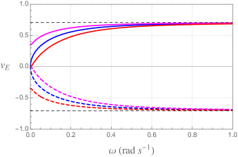
Figure 9: Energy velocity $V_{E}^{+}$ and $\widetilde{V}_{E}^{+}$ of Eq. (92a). The particular cases considered here are: $\theta=\pi/2$ (blue), $\theta=0$ (red), and $\theta=\pi$ (magenta). Solid (dashed) lines indicate $V_{E}^{+}(\widetilde{V}_{E}^{+})$, respectively. Here we have used $\mu=1$, $\epsilon^{\prime}=2$, $\sigma=0.8$ $\mathrm{s}^{-1}$, $|{\bf{a}}\times{\bf{c}}|=0.3$ $\mathrm{s}^{-1}$.

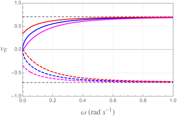
Figure 10: Energy velocity $V_{E}^{-}$ and $\widetilde{V}_{E}^{-}$ of Eq. (92a).The particular cases considered are: $\theta=\pi/2$ (blue), $\theta=0$ (red), and $\theta=\pi$ (magenta). Solid (dashed) curves represent $V_{E}^{-}$ $(\widetilde{V}_{E}^{-})$. Here we have used $\mu=1$, $\epsilon^{\prime}=2$, $\sigma=0.8$ $\mathrm{s}^{-1}$, $|{\bf{a}}\times{\bf{c}}|=0.3$ $\mathrm{s}^{-1}$.

Notice that if ${\bf a}$ is parallel (or anti-parallel) to ${\bf c}$, the contribution of the magnetic conductivity tensor is null in the result (87). Furthermore, the dispersion relation (87) is equivalent to the dispersion equation (69) of the antisymmetric case by replacing $\pm({\bf a}\times{\bf c})/2\rightarrow{\bf b}$, which assures similarity of results with the ones of the previous section.

By calculating the differential in relation to $k^{i}$-component in Eq. (87), the corresponding group velocity is

$${\bf v}_{g}^{\pm}=\frac{\partial\omega}{\partial{\bf k}}=\frac{\displaystyle\frac{{\bf k}}{\mu\omega}\pm i\,\frac{({\bf a\times c})}{4\omega}}{\displaystyle\left(\epsilon^{\prime}+\frac{\omega}{2}\frac{\partial\epsilon^{\prime}}{\partial\omega}\right)+i\left(\epsilon^{\prime\prime}+\frac{\omega}{2}\frac{\partial\epsilon^{\prime\prime}}{\partial\omega}\right)}\;,$$ (93)

which is valid for all frequency range, and for both solutions $k_{\pm}$ and $\tilde{k}_{\pm}$. Let us now writing the $k^{i}$-components as $k^{i}=k^{\prime i}+ik^{\prime\prime i}$, then the group velocity can be rewritten as

$${\bf v}_{g}^{\pm} =\frac{\displaystyle\frac{{\bf k}^{\prime}}{\mu\omega}+i\,\frac{\omega\epsilon^{\prime\prime}\,\hat{{\bf k}}}{2k^{\prime}}}{\displaystyle\left(\epsilon^{\prime}+\frac{\omega}{2}\frac{\partial\epsilon^{\prime}}{\partial\omega}\right)+i\left(\epsilon^{\prime\prime}+\frac{\omega}{2}\frac{\partial\epsilon^{\prime\prime}}{\partial\omega}\right)}\;.$$ (94)

Similarly to the antisymmetric case of Sec. III.2, we observe that for a non absorbing scenario, $\epsilon^{\prime\prime}=0$ and $|{\bf{a}}\times{\bf{c}}|\cos\varphi=0$, one has $V_{E}^{\pm}=v_{g}^{\pm}$.

Furthermore, in the case of the magnetically induced absorption, $\epsilon^{\prime\prime}=0$ and $|{\bf{a}}\times{\bf{c}}|\cos\varphi\neq 0$, one also finds

$$v_{g}^{\pm}=V_{E}^{\pm}=\frac{{k^{\prime}_{\pm}}/{\mu\omega}}{\displaystyle\epsilon^{\prime}+\frac{\omega}{2}\frac{\partial\epsilon^{\prime}}{\partial\omega}}\;,$$ (95)

where, in this case,

$$k^{\prime}_{\pm}=\omega S_{+},\quad S_{\pm}=\frac{1}{\sqrt{2}}\sqrt{|g(\omega)|\left(1\pm\mathrm{sgn}[g(\omega)]\right)}\;,$$ (96)

such that,

$$v_{g}^{\pm}=V_{E}^{\pm}=\frac{\sqrt{|g(\omega)|\left(1+\mathrm{sgn}[g(\omega)]\right)}}{\displaystyle\mu\sqrt{2}\left(\epsilon^{\prime}+\frac{\omega}{2}\frac{\partial\epsilon^{\prime}}{\partial\omega}\right)}\;.$$ (97)

Again, we observe that

• For $g(\omega)>0$, one has $\mathrm{sgn}[g(\omega)]=1$, which yields

  $$v_{g}^{\pm}=V_{E}^{\pm}=\frac{\sqrt{|g(\omega)|}}{\displaystyle\mu\left(\epsilon^{\prime}+\frac{\omega}{2}\frac{\partial\epsilon^{\prime}}{\partial\omega}\right)}\;.$$ (98)

• For $g(\omega)<0$, which occurs for $0<\omega<\omega^{\prime\prime}$, with

  $$\omega^{\prime\prime} =\sqrt{\frac{\mu|{\bf{a}}\times{\bf{c}}|^{2}\cos^{2}\varphi}{16\epsilon^{\prime}}}\;,$$ (99)

  there occurs $\mathrm{sgn}[g(\omega)]=-1$, leading to $S_{+}=0$, and

  $$v_{g}^{\pm}=V_{E}^{\pm}=0\;.$$ (100)

This same analysis also holds for the energy velocity $\widetilde{V}_{E}^{\pm}$ associated with $\tilde{k}_{\pm}$, since $\tilde{k}_{\pm}^{\prime}=-\omega S_{+}$. We illustrate the behavior of the energy velocities for $\epsilon^{\prime\prime}=0$ and $|{\bf{a}}\times{\bf{c}}|\cos\varphi\neq 0$ in the Fig. 11, considering the parallel and antiparallel configurations.

Figure 11: Energy velocity $V_{E}^{\pm}$ of Eq. (92a) for $\epsilon^{\prime\prime}=0$. Solid red line indicates $V_{E}^{\pm}$ for $\theta={0,\pi}$, while the dashed red curve represents $\widetilde{V}_{E}^{\pm}$ for $\theta={0,\pi}$. Here we have used $\mu=1$, $\epsilon^{\prime}=2$, $b=0.3$ $\mathrm{s}^{-1}$. The vertical dashed line indicates the frequency $\omega^{\prime\prime}$ of Eq. (99).

IV Final remarks

In this work, we have investigated a dielectric medium endowed with magnetic conductivity, concerning optical effects and electromagnetic signal propagation. Considering special cases for the magnetic conductivity, we have obtained the polarization of the collective electromagnetic propagating modes and their related refractive indices. We also have presented the solutions that describe negative refraction in each case. Furthermore, analyses of optical properties were carried out. For the isotropic magnetic conductivity of Sec. II.1, we determined the rotatory power, while the phase shift and absorption coefficients for the antisymmetric conductivity were found in Sec. II.2. Finally, the symmetric conductivity was addressed in Sec. II.3, where the phase shift and absorption difference (per unit length) between propagating modes were achieved.

In Sec. III, we have investigated aspects regarding the propagation of electromagnetic energy. In doing so, we have obtained the energy velocity of the modes (related to positive and negative refraction). As expected, the energy velocity is negative for the negative refraction propagating modes. In this context, we have obtained some peculiar and surprising outcomes when comparing energy velocity and group velocity. For general non-absorbing media, it is known in the literature that energy velocity and group velocity are equivalent, whereas for absorbing media such equivalence is lost. However, our results revealed that, when the dispersive dielectric is endowed with magnetic conductivity, the latter statements are no longer valid. Indeed, for the isotropic conductivity of Sec. III.1, in the absence of absorption $(\epsilon^{\prime\prime}=0,\Sigma\neq 0)$, one finds that $v_{g}\neq v_{E}$, “breaking” the equivalence between energy and group velocities for a real refractive index medium. Such a situation is represented in the first line, second column of Table 1.

For the anisotropic and non-diagonal conductivities, namely, the antisymmetric and symmetric cases of Secs. III.2 and III.3, respectively, there occurs the magnetically induced absorption, that is, the refractive indices become complex, even when $\epsilon^{\prime\prime}=0$, due to the non-null magnetic conductivity, as we can see in Eq. (72) and Eq. (89). For both cases, it holds $v_{g}=V_{E}$ in spite of the associated complex refractive indices. In such cases, only when $\epsilon^{\prime\prime}\neq 0$ the energy velocity will be different from the group velocity. These cases are represented in the second and third lines of the second column of Table 1.

These bold and surprising distinctions indicate that dispersive media endowed with magnetic conductivity have specific energy propagation properties, which seem to be not described by the usual formalism. All results regarding the group velocity and energy velocity in dispersive media endowed with magnetic conductivity are displayed in Table 1.

Table 1: Comparison of group and energy velocities in the cases of isotropic, antisymmetric, and symmetric magnetic conductivity tensors. Note that the unexpected results are the ones in the second column, highlighted in blue color.

	$(\epsilon^{\prime\prime}\neq 0,\hskip 5.69046pt\sigma^{B}_{ij}\neq 0)$	$(\epsilon^{\prime\prime}=0,\hskip 5.69046pt\sigma^{B}_{ij}\neq 0)$	$(\epsilon^{\prime\prime}=0,\hskip 5.69046pt\sigma^{B}_{ij}=0)$
$\sigma^{B}_{ij}=\Sigma\,\delta_{ij}$	$v_{g}\neq V_{E}$ $|$   $n\in\mathbb{C}$	$v_{g}\neq V_{E}$ $|$   $n\in\mathbb{R}$	$v_{g}=V_{E}$ $|$   $n\in\mathbb{R}$
$\sigma^{B}_{ij}=\epsilon_{ijk}\,b_{k}$	$v_{g}\neq V_{E}$ $|$   $n\in\mathbb{C}$	$v_{g}=V_{E}$ $|$   $n\in\mathbb{C}$	$v_{g}=V_{E}$ $|$   $n\in\mathbb{R}$
$\sigma^{B}_{ij}=(a_{i}\,c_{j}+a_{j}\,c_{i})/2$	$v_{g}\neq V_{E}$ $|$   $n\in\mathbb{C}$	$v_{g}=V_{E}$ $|$   $n\in\mathbb{C}$	$v_{g}=V_{E}$ $|$   $n\in\mathbb{R}$

- [1] D.E. Kharzeev, The chiral magnetic effect and anomaly-induced transport, Prog. Part. Nucl. Phys. 75, 133 (2014); D.E. Kharzeev, J. Liao, S.A. Voloshin, and G. Wang, Chiral magnetic and vortical effects in high-energy nuclear collisions – A status report, Prog. Part. Nucl. Phys. 88, 1 (2016); D. Kharzeev, K. Landsteiner, A. Schmitt and H.U. Yee, Strongly Interacting Matter in Magnetic Fields, Lect. Notes Phys. 871 (Springer-Verlag, Berlin Heidelberg, 2013).
- [2] K. Fukushima, D.E. Kharzeev, and H.J. Warringa, Chiral magnetic effect, Phys. Rev. D 78, 074033 (2008).
- [3] G. Inghirami, M. Mace, Y. Hirono, L. Del Zanna, D.E. Kharzeev, and M. Bleicher, Magnetic fields in heavy ion collisions: flow and charge transport, Eur. Phys. J. C 80, 293 (2020).
- [4] J. Schober, A. Brandenburg and I. Rogachevskii, Chiral fermion asymmetry in high-energy plasma simulations, Geophys. Astrophys. Fluid Dynamics 114, 106 (2020).
- [5] A. Vilenkin, Equilibrium parity-violating current in a magnetic field, Phys. Rev. D 22, 3080 (1980); A. Vilenkin and D.A. Leahy, Parity nonconservation and the origin of cosmic magnetic fields, Astrophys. J. 254, 77 (1982).
- [6] M. Dvornikov and V.B. Semikoz, Influence of the turbulent motion on the chiral magnetic effect in the early universe, Phys. Rev. D 95, 043538 (2017).
- [7] G. Sigl and N. Leite, Chiral magnetic effect in protoneutron stars and magnetic field spectral evolution, JCAP 01, 025 (2016).
- [8] M. Dvornikov and V.B. Semikoz, Magnetic field instability in a neutron star driven by the electroweak electron-nucleon interaction versus the chiral magnetic effect, Phys. Rev. D 91, 061301(R) (2015).
- [9] A.F. Bubnov, N.V. Gubina, and V.Ch. Zhukovsky, Vacuum current induced by an axial-vector condensate and electron anomalous magnetic moment in a magnetic field, Phys. Rev. D 96, 016011 (2017).
- [10] Y. Akamatsu and N. Yamamoto, Chiral Plasma Instabilities, Phys. Rev. Lett. 111, 052002 (2013); A. Boyarsky, O. Ruchayskiy, and M. Shaposhnikov, Long-Range Magnetic Fields in the Ground State of the Standard Model Plasma, Phys. Rev. Lett. 109, 111602 (2012).
- [11] M. Dvornikov and V.B. Semikoz, Instability of magnetic fields in electroweak plasma driven by neutrino asymmetries, JCAP 05, 002 (2014); M. Dvornikov, Chiral magnetic effect in the presence of an external axial-vector field, Phys. Rev. D 98, 036016 (2018).
- [12] M. Dvornikov, Electric current induced by an external magnetic field in the presence of electroweak matter, EPJ Web Conf. 191, 05008 (2018).
- [13] A.A. Burkov, Chiral anomaly and transport in Weyl metals, J. Phys. Condens. Matter 27, 113201 (2015).
- [14] Q. Li, D.E. Kharzeev, C. Zhang, Y. Huang, I. Pletikosić, A.V. Fedorov, R.D. Zhong, J.A. Schneeloch, G.D Gu, and T. Valla, Chiral magnetic effect in , Nature Phys. 12, 550 (2016).
- [15] M.-C. Chang and M.-F. Yang, Chiral magnetic effect in a two-band lattice model of Weyl semimetal, Phys. Rev. B 91, 115203 (2015).
- [16] E.C.I van der Wurff and H.T.C. Stoof, Anisotropic chiral magnetic effect from tilted Weyl cones, Phys. Rev. B 96, 121116(R) (2017).
- [17] K. Landsteiner, Anomalous transport of Weyl fermions in Weyl semimetals, Phys. Rev. B 89, 075124 (2014).
- [18] S. Kaushik and D.E. Kharzeev, Quantum oscillations in the chiral magnetic conductivity, Phys. Rev. B 95, 235136 (2017).
- [19] A. Martín-Ruiz, M. Cambiaso, and L.F. Urrutia, Electromagnetic fields induced by an electric charge near a Weyl semimetal, Phys. Rev. B 99, 155142 (2019).
- [20] D.E. Kharzeev and H.J. Warringa, Chiral magnetic conductivity, Phys. Rev. D 80, 034028 (2009); D.E. Kharzeev, Chiral magnetic superconductivity, EPJ Web Conf. 137, 01011 (2017).
- [21] S.M. Carroll, G.B. Field, and R. Jackiw, Limits on a Lorentz- and parity-violating modification of electrodynamics, Phys. Rev. D 41, 1231 (1990).
- [22] D. Colladay and V.A. Kostelecký, CPT violation and the standard model, Phys. Rev. D 55, 6760 (1997); Lorentz-violating extension of the standard model, Phys. Rev. D 58, 116002 (1998); V.A. Kostelecký and M. Mewes, Signals for Lorentz violation in electrodynamics, Phys. Rev. D 66, 056005 (2002).
- [23] Z. Qiu, G. Cao and X.-G. Huang, Electrodynamics of chiral matter, Phys. Rev. D 95, 036002 (2017).
- [24] F. Wilczek, Two Applications of Axion Electrodynamics, Phys. Rev. Lett. 58, 1799 (1987).
- [25] K. Deng, J. S. Van Dyke, D. Minic, J. J. Heremans, and E. Barnes, Exploring self-consistency of the equations of axion electrodynamics in Weyl semimetals, Phys. Rev. B 104, 075202 (2021).
- [26] E. Barnes, J. J. Heremans, and Djordje Minic, Electromagnetic Signatures of the Chiral Anomaly in Weyl Semimetals, Phys. Rev. Lett. 117, 217204 (2016).
- [27] A. Sekine and K. Nomura, Axion electrodynamics in topological materials, J. Appl. Phys. 129, 141101 (2021).
- [28] M. E. Tobar, B. T. McAllister, and M. Goryachev, Modified axion electrodynamics as impressed electromagnetic sources through oscillating background polarization and magnetization, Phys. Dark Universe 26, 100339 (2019).
- [29] P. D. S. Silva, L. L. Santos, M. M. Ferreira, Jr., and M. Schreck, Effects of CPT-odd terms of dimensions three and five on electromagnetic propagation in continuous matter, Phy. Rev. D 104, 116023 (2021).
- [30] L. C. T. Brito, J. C. C. Felipe, A. Yu. Petrov, A. P. Baeta Scarpelli, No radiative corrections to the Carroll-Field-Jackiw term beyond one-loop order, Int. J. Mod. Phys. A36, 2150033 (2021); J. F. Assuncao, T. Mariz, A. Yu. Petrov, Nonanalyticity of the induced Carroll-Field-Jackiw term at finite temperature, EPL 116, 31003 (2016); J. C. C. Felipe, A. R. Vieira, A. L. Cherchiglia, A. P. Baêta Scarpelli, M. Sampaio, Arbitrariness in the gravitational Chern-Simons-like term induced radiatively, Phys. Rev. D 89, 105034 (2014); T.R.S. Santos, R.F. Sobreiro, Lorentz-violating Yang–Mills theory: discussing the Chern–Simons-like term generation, Eur. Phys. J. C 77, 903 (2017).
- [31] R. Casana, M. M. Ferreira Jr., E. da Hora, A. B. F. Neves, Maxwell-Chern-Simons vortices in a CPT-odd Lorentz-violating Higgs Electrodynamics, Eur. Phys. J. C 74, 3064 (2014); R. Casana, L. Sourrouille, Self-dual Maxwell-Chern-Simons solitons from a Lorentz-violating model, Phys. Lett. B 726, 488 (2013).
- [32] H. Belich, L. D. Bernald, Patricio Gaete, J. A. Helayël-Neto, The photino sector and a confining potential in a supersymetric Lorentz-symmetry-violating model, Eur. Phys. J. C 73, 2632 (2013); L. Bonetti, L. R. dos Santos Filho, J A. Helayël-Neto, A. D. A. M. Spallicci, Photon sector analysis of Super and Lorentz symmetry breaking: effective photon mass, bi-refringence and dissipation, Eur. Phys. J. C 78, 811 (2018).
- [33] Y. M. P. Gomes, P. C. Malta, Lab-based limits on the Carroll-Field-Jackiw Lorentz-violating electrodynamics, Phys. Rev. D 94, 025031 (2016); M.M. Ferreira Jr, J.A. Helayël-Neto, C.M. Reyes, M. Schreck, P.D.S. Silva, Unitarity in Stückelberg electrodynamics modified by a Carroll-Field-Jackiw term, Phys. Lett. B 804, 135379 (2020); A. Martín-Ruiz and C. A. Escobar, Local effects of the quantum vacuum in Lorentz-violating electrodynamics, Phys. Rev. D 95, 036011 (2017).
- [34] Q.G. Bailey and V.A. Kostelecký, Lorentz-violating electrostatics and magnetostatics, Phys. Rev. D 70, 076006 (2004).
- [35] A. Gomez, A. Martín-Ruiz, Luis F. Urrutia, Effective electromagnetic actions for Lorentz violating theories exhibiting the axial anomaly, Phys. Lett. B 829, 137043 (2022).
- [36] A. V. Kostelecky, R. Lehnert, N. McGinnis, M. Schreck, B. Seradjeh, Lorentz violation in Dirac and Weyl semimetals, Phys. Rev. Research 4, 023106 (2022).
- [37] P.D.S. Silva, M.M. Ferreira Jr., M. Schreck, and L.F. Urrutia, Magnetic-conductivity effects on electromagnetic propagation in dispersive matter, Phys. Rev. D 102, 076001 (2020).
- [38] S. Kaushik, D.E. Kharzeev, and E.J. Philip, Transverse chiral magnetic photocurrent induced by linearly polarized light in symmetric Weyl semimetals, Phys. Rev. Research 2, 042011(R) (2020).
- [39] J. D. Jackson, Classical Electrodynamics, 3rd eddition. New York (USA): John Wiley & Sons, 1999.
- [40] A. Zangwill, Modern Electrodynamics. New York (USA): Cambridge University Press, 2012.
- [41] L.D. Landau and E.M. Lifshitz, Electrodynamics of continuous media, Course of Theoretical Physics, Volume 8, 2nd ed. (Pergamon Press, New York, 1984).
- [42] E. Sonnenschein, I. Rutkevich, and D. Censor, Wave packets, rays, and the role of real group velocity in absorbing media, Phys. Rev. E 57, 1005 (1997).
- [43] J. Neufeld, Wave propagation and group velocity in absorbing media, Phys. Lett. A Phys. 29, 68 (1969).
- [44] R. Loudon, The propagation of electromagnetic energy through an absorbing dielectric, J. Phys. A: Gen. Phys.3, 233 (1970).
- [45] G. C. Sherman and K. E. Oughstun, Energy-velocity description of pulse propagation in absorbing, dispersive dielectrics, J. Opt. Soc. Am. B 12, 229-247 (1995).
- [46] M.V. Davidovich, Electromagnetic energy density and velocity in a medium with anomalous positive dispersion, Tech. Phys. Lett. 32, 982–986 (2006).
- [47] R. Ruppin, Electromagnetic energy density in a dispersive and absorptive material, Phys. Lett. A 299, 309-312 (2002).
- [48] V. Gerasik and M. Stastna, Complex group velocity and energy transport in absorbing media, Phys. Rev. E 81, 056602 (2010).
- [49] E. Hecht, Optics, 4th ed. (Addison Wesley, San Francisco, 2002).