A multipoint perturbation formula
for eigenvalue problems

Abstract.

Standard perturbation theory of eigenvalue problems consists of obtaining approximations of eigenmodes in the neighborhood of a Hamiltonian where the corresponding eigenmode is known. Nevertheless, if the corresponding eigenmodes of several nearby Hamiltonians are known, standard perturbation theory cannot simultaneously use all this knowledge to provide a better approximation. We derive a formula enabling such an approximation result, and provide numerical examples for which this method is more competitive than standard perturbation theory.

1. Introduction

Eigenvalue problems are ubiquitous in applied mathematics, for instance in quantum physics, structural mechanics, graph theory and optimization. Numerical methods to solve these eigenvalue problems are hence key to obtain accurate approximate solutions in an efficient and robust way. Let us take a Hilbert space, consider $H^{0}$ to be a self-adjoint operator on this Hilbert space, and define a family of self-adjoint operators

$$H(G):=H^{0}+G$$

called Hamiltonians, where $G$ is a parametrized self-adjoint operator. We consider the eigenvalue problem associated to $H(G)$ under variation of $G$. A widely used approach to treat eigenvalue problems is based on perturbation theory, where one knows or can easily compute the eigenstates of an operator $H(G_{1})$ for some $G_{1}$ and deduces properties of approximate solutions for the close problem $H(G_{1})+g$, where $g$ is small in some sense to be made precise later, see [2, 1, 3] and [7, Section XII] for a presentation of perturbation theory for eigenvalue problems. In other words, from spectral information on $H(G_{1})$, one can deduce information on the perturbed $H(G_{1})+g$ for small perturbations $g$, thus locally around $H(G_{1})$.

In contrast, when the solution of an eigenvalue problem with Hamiltonian $H(G_{j})$ is known at $n$ points $\left(G_{j}\right)_{j=1}^{n}$, standard perturbation theory does not exploit the full approximation power of using the information at all $n$ points to obtain approximations at a new point $G$ as it will only use local information of the closest point $G_{j}$. We illustrate the comparison between single point and multipoint perturbation theory on Figure 1.

Figure 1. In standard perturbation theory, one gets approximations of the solution $\mathcal{F}(G)$ at a new point $G$ by using only the closest $G_{j}$ on which we know the solution $\mathcal{F}(G_{j})$, while in multipoint perturbation we simultaneously use all the $G_{j}$’s on which we know the solutions.

Let us now detail our framework. We consider some admissible set $\mathcal{G}$ of operators $G$’s, being the space of parameters for the Hamiltonian. For $G\in\mathcal{G}$ and $k\in\mathbb{N}\backslash\{0\}$, we denote by $\mathcal{F}\left(G\right)$ the spectral projection onto the eigenspace corresponding to the $k^{\text{th}}$ lowest eigenvalue of the operator $H(G)$, which we assume to be non-degenerate. It is clear that the knowledge of $\mathcal{F}(G)$ is equivalent to know an eigenvector corresponding to the $k^{\text{th}}$ eigenvalue. Our framework can be generalized to projectors onto the space generated by several eigenvalues, and those eigenvalues could lie anywhere in the discrete spectrum since our methodology relies on spectral projectors, or, in other words, on density matrices for the selected states. However, this goes beyond the scope of this work and we restrict our analysis within this article to the non-degenerate case.

The motivation for this work comes from [4, 5], where it is observed that if $G$ is a linear combination of $G_{j}$’s, that is

$$G=\sum_{j=1}^{n}\alpha_{j}G_{j},$$

then the density matrix appears to be well approximated by the same linear combination of the corresponding density matrix, i.e.

$$\mathcal{F}(G)\simeq\sum_{j=1}^{n}\alpha_{j}\mathcal{F}(G_{j}).$$

This amounts to say that the map $G\mapsto\mathcal{F}(G)$ is locally very close to linear, under some conditions. In this work, we aim at partly explaining this phenomenon developping a multipoint perturbation theory (a precise meaning will be given later).

This article is organized as follows. In Section 2, we provide the mathematical setting and present a review of standard perturbation theory. In Section 3, we present our main result, the resolvent formula (13), and compute the first orders in the expansion of $\mathcal{F}(G)$ in Section 4. We illustrate our work with numerical simulations on Schrödinger operators in Section 5. We conclude that the produced approximations are particularly relevant when the $G_{j}$’s are close to each other, and when the $G$ on which one wants the solution is close to the affine space spanned by the $G_{j}$’s. All the proofs are provided in Section 6.

2. Mathematical setting

In this section, we define the main mathematical objects that will be needed later on for the presentation of the multipoint perturbation method itself and the theoretical analysis that follows.

2.1. Hamiltonians

First, we consider a separable Hilbert space $\mathcal{H}$ endowed with a scalar product $\left<\cdot,\cdot\right>$, with corresponding norm $\|\cdot\|$. Inequalities on operators will be considered in the sense of forms, meaning that for two operators $A$ and $B$, we write $A\leqslant B$ if there is a vector subspace $\mathcal{H}_{0}\subset\mathcal{H}$, dense in $\mathcal{H}$, such that $\left<\psi,A\psi\right>\leqslant\left<\psi,B\psi\right>$ for all $\psi\in\mathcal{H}_{0}$. We consider a self-adjoint operator $H^{0}$ on $\mathcal{H}$, satisfying $H^{0}\geqslant\alpha$ for some $\alpha\in\mathbb{R}_{+}$. Throughout the paper, $H^{0}$ will be a fixed operator, for instance $-\Delta$ in the case of Schrödinger operators. Moreover, for a given operator $A$, we denote its adjoint operator by $A^{*}$.

We define the set of admissible perturbations by

$$\mathcal{G}:=\big{\{}G\text{ linear operator on }\mathcal{H},\;G^{*}=G,\;\forall\varepsilon>0\;\exists c^{G}_{\varepsilon}>0,\;\left|G\right|\leqslant\varepsilon H^{0}+c^{G}_{\varepsilon}\big{\}},$$ (1)

where $|A|:=\sqrt{A^{*}A}$ is defined via the spectral theorem. For any $G\in\mathcal{G}$, by the Kato–Lions–Lax–Milgram–Nelson (KLMN) theorem [6, p. 323], the Friedrichs extension of

$$H(G)=H^{0}+G$$

is a well-defined self-adjoint and bounded from below operator. Considering the set (1) enables to take into account Schrödinger operators perturbed by, e.g., singular potentials. We could also treat operators $H(G)$ which are not bounded from below, this extension is immediate from our presentation.

The finite-dimensional case is covered by our analysis as we make no assumption whether the Hilbert space is finite or infinite-dimensional. In the finite-dimensional case, $\mathcal{G}$ is the space of $m\times m$ matrices, where $m$ is the dimension of the considered Hilbert space.

2.2. Non-degeneracy assumption

We use the notation $\mathbb{N}=\{0,1,\dots\}$, so $0\in\mathbb{N}$, and we will use the notation $\mathbb{N}\backslash\{0\}$ for the set of strictly positive integers. Since we only consider non-degenerate eigenmodes, we take $k\in\mathbb{N}\backslash\{0\},$ fixed throughout all the document. Moreover, in all this article, for any $G\in\mathcal{G}$ and any $p\in\mathbb{N}\backslash\{0\}$, we denote by $\lambda^{p}(G)$ the $p^{\text{th}}$ eigenvalue of $H(G)$, counting multiplicities.

For any $\left(G_{j}\right)_{j=1}^{n}\in\mathcal{G}^{n}$, we assume that the $k^{\text{th}}$ eigenvalue is always separated from the rest of the spectrum, and that it remains so as we navigate on the corresponding admissible space. To translate this into mathematical terms, we first define for any $\lambda_{\textup{min}},\lambda_{\textup{max}}\in\mathbb{R}$ the set

$$\Omega_{\lambda_{\textup{min}}}^{\lambda_{\textup{max}}}:=\left\{G\in\mathcal{G}\;\middle|\;\sigma(H(G))\cap[\lambda_{\textup{min}},\lambda_{\textup{max}}]=\{\lambda^{k}(G)\}\right\},$$ (2)

where $\sigma(A)$ denotes the spectrum of $A$ for any operator $A$. We then formalize the following assumption.

Assumption 2.1.

There holds

$$\exists\lambda_{\textup{min}},\lambda_{\textup{max}}\in\mathbb{R},\;\lambda_{\textup{min}}<\lambda_{\textup{max}},\qquad\mbox{such that}\qquad\text{Conv }\left(G_{j}\right)_{j=1}^{n}\subset\Omega_{\lambda_{\textup{min}}}^{\lambda_{\textup{max}}},$$ (3)

where “Conv” denotes the convex hull.

In the following, we will consider $G$’s such that

$$G\in\Omega_{\lambda_{\textup{min}}}^{\lambda_{\textup{max}}}.$$

Moreover, in all this document, $\mathcal{C}\subset\mathbb{C}$ will denote a contour, say a rectangle, such that $\mathcal{C}\cap\mathbb{R}=\{\lambda_{\textup{min}},\lambda_{\textup{max}}\}$. From Assumption 2.1, this contour will enclose exactly one eigenvalue of $H(G)$, namely the $k^{\text{th}}$ eigenvalue, for any $G\in\Omega_{\lambda_{\textup{min}}}^{\lambda_{\textup{max}}}$.

2.3. Operator norms

Take $\mu\in\;]-\inf\sigma(H^{0}),+\infty[$, and $\kappa\in[0,1]$. For any operator on $\mathcal{H}$, we define the operator norm as

$$\left|\!\left|A\right|\!\right|:=\left|\!\left|A\right|\!\right|_{\mathcal{H}\rightarrow\mathcal{H}}=\underset{\begin{subarray}{c}\psi\in\mathcal{H}\\ \psi\neq 0\end{subarray}}{\text{{sup}}}\quad\frac{\left|\!\left|A\psi\right|\!\right|}{\left|\!\left|\psi\right|\!\right|},$$

which can be equal to $+\infty$. The set $\{A:\mathcal{H}\rightarrow\mathcal{H}\;|\;\left|\!\left|A\right|\!\right|<+\infty\}$ is usually denoted by $\mathcal{L}(\mathcal{H})$. We define, for any operator $\Gamma$ of $\mathcal{H}$,

$$\left|\!\left|\Gamma\right|\!\right|_{e}:=\left|\!\left|\left(H^{0}+\mu\right)^{\frac{\kappa}{2}}\;\Gamma\;\left(H^{0}+\mu\right)^{\frac{\kappa}{2}}\right|\!\right|$$ (4)

which will be the norm on the space of density matrices. The norm on the parameter space is the dual one, which is given by,

$$\left|\!\left|G\right|\!\right|_{a}:=\left|\!\left|\left(H^{0}+\mu\right)^{-\frac{\kappa}{2}}\;G\;\left(H^{0}+\mu\right)^{-\frac{\kappa}{2}}\right|\!\right|,$$ (5)

defined for any operator $G$ of $\mathcal{H}$. Taking $\kappa=1$ is the most natural choice from a theoretical point of view since $\left|\!\left|\cdot\right|\!\right|_{e}$ becomes the natural energy norm in this case. However, the following proofs work for any $\kappa\in[0,1]$. In the numerical section, we will also take $\kappa=1$, but one could consider $\kappa=0$ to simplify the implementation.

2.4. Resolvents and density matrices

Let $\mathcal{C}$ be the contour introduced in Section 2.2 relying on Assumption 2.1 and take $G\in\Omega_{\lambda_{\textup{min}}}^{\lambda_{\textup{max}}}$. Given the resolvent $\left(z-H(G)\right)^{-1}$ of $H(G)$, we define

$$\mathcal{F}(G):=\frac{1}{2\pi i}\oint_{\mathcal{C}}\left(z-H(G)\right)^{-1}{\rm d}z.$$ (6)

By the spectral theorem, see [7, Section XII], $\mathcal{F}(G)$ is the spectral projection onto the one-dimensional space spanned by an eigenvector corresponding to the $k^{\text{th}}$ eigenvalue of $H(G)$.

2.5. Pseudo-inverses

We consider $G\in\mathcal{G}$ and Assumption 2.1 of Section 2.2, where a level $k\in\mathbb{N}\backslash\{0\}$ was defined. We now introduce the pseudo-inverse operator

$$K(G):=\left\{\begin{array}[]{ll}\left(\left(\lambda^{k}(G)-H(G)\right)_{\mkern 1.0mu\vrule height=6.02777pt\mkern 2.0mu\left(\operatorname{Ker}\left(\lambda^{k}(G)-H(G)\right)\right)^{\perp}}\right)^{-1}&\mbox{on }\left(\operatorname{Ker}\left(\lambda^{k}(G)-H(G)\right)\right)^{\perp},\\ 0&\mbox{on }\operatorname{Ker}\left(\lambda^{k}(G)-H(G)\right),\end{array}\right.$$ (9)

extended on the whole of $\mathcal{H}$ by linearity, that will be needed in the upcoming perturbation theory. We recall that $\operatorname{Ker}\left(\lambda^{k}(G_{j})-H(G_{j})\right)$ is the one-dimensional vector space spanned by an eigenvector corresponding to the $k^{\text{th}}$ eigenvalue of $H(G_{j})$.

Let us illustrate this definition for a finite-dimensional Hilbert space $\mathcal{H}$. In this case, $H(G)$ is a hermitian matrix, and taking $\left(u_{a}(G)\right)_{a=1}^{\dim\mathcal{H}}$ a basis of $\mathcal{H}$ formed by eigenvectors of $H(G)$ sorted such that the corresponding eigenvalues $\left(\lambda^{a}(G)\right)_{a=1}^{\dim\mathcal{H}}$ are increasing, provides the explicit representation for the pseudo-inverse

$$K(G)=\sum_{\begin{subarray}{c}1\leqslant a\leqslant\dim\mathcal{H}\\ a\neq k\end{subarray}}\left(\lambda^{k}(G)-\lambda^{a}(G)\right)^{-1}P_{u_{a}(G)},$$

where $P_{u}$ is the projection operator on the vector space spanned by $u\in\mathcal{H}$.

2.6. Standard linear perturbation theory

We now present standard perturbation theory, in the aim of comparing it with the proposed multipoint perturbation method. Let us take $G_{1}\in\mathcal{G}$, consider the non-degeneracy assumption 2.1 and take $G\in\Omega_{\lambda_{\textup{min}}}^{\lambda_{\textup{max}}}$. We consider that the unperturbed operator is $H(G_{1})$ i.e. we assume knowledge of $P_{1}:=\mathcal{F}(G_{1})$ and $K_{1}:=K(G_{1})$ using (9). Standard perturbation theory consists in deducing approximations of $\mathcal{F}(G)$ in series of $G-G_{1}$. The base resolvent equation is

$$\left(z-H(G)\right)^{-1}=\left(z-H(G_{1})\right)^{-1}\left(1-(G-G_{1})\left(z-H(G_{1})\right)^{-1}\right)^{-1}.$$ (10)

We then define for $\ell\in\mathbb{N}$,

$$\mathcal{P}_{\ell}:=\frac{1}{2\pi i}\oint_{\mathcal{C}}(z-H(G_{1}))^{-1}\left((G-G_{1})(z-H(G_{1}))^{-1}\right)^{\ell}{\rm d}z,\qquad\mathbb{P}_{\ell}:=\sum_{p=0}^{\ell}\mathcal{P}_{p},$$

and recall the following classical result [2, 7].

Proposition 2.2 (Standard linear perturbation theory bound).

Take $k\in\mathbb{N}\backslash\{0\}$, $G_{1},G\in\mathcal{G}$ satisfying the non-degeneracy assumption 2.1, consider the contour $\mathcal{C}$ as in Section 2.2, define $g:=G-G_{1}$ and $C:=\max_{z\in\mathcal{C}}\left|\!\left|\left(z-H(G_{1})\right)^{-1}\right|\!\right|_{e}$, and assume that $\left|\!\left|g\right|\!\right|_{a}<1/(2C)$. Then there exists a constant $c>0$ independent of $g$ and $\ell$ such that for any $\ell\in\mathbb{N}$,

$$\left|\!\left|\mathcal{F}(G)-\mathbb{P}_{\ell}\right|\!\right|_{e}\leqslant c\left(C\left|\!\left|g\right|\!\right|_{a}\right)^{\ell+1}.$$ (11)

For the sake of completeness, we provide a proof in Section 6. The terms $\mathbb{P}_{\ell}$ can be obtained explicitly using Cauchy’s integration formula. For instance, the four first order terms read

$$\mathcal{P}_{0} =P_{1},$$ (12)

$$\mathcal{P}_{1} =P_{1}gK_{1}+K_{1}gP_{1},$$

$$\mathcal{P}_{2} =\left(P_{1}gK_{1}gK_{1}+K_{1}gP_{1}gK_{1}+K_{1}gK_{1}gP_{1}\right)-(P_{1}gP_{1}gK_{1}^{2}+P_{1}gK_{1}^{2}gP_{1}+K_{1}^{2}gP_{1}gP_{1}),$$

$$\mathcal{P}_{3} =(P_{1}gP_{1}gP_{1}gK_{1}^{3}+P_{1}gP_{1}gK_{1}^{3}gP_{1}+P_{1}gK_{1}^{3}gP_{1}gP_{1}+K_{1}^{3}gP_{1}gP_{1}gP_{1})$$

$$\qquad+(P_{1}gK_{1}gK_{1}gK_{1}+K_{1}gP_{1}gK_{1}gK_{1}+K_{1}gK_{1}gP_{1}gK_{1}+K_{1}gK_{1}gK_{1}gP_{1})$$

$$\qquad-\left(P_{1}gP_{1}gK_{1}^{2}gK_{1}+P_{1}gP_{1}gK_{1}gK_{1}^{2}+K_{1}gK_{1}^{2}gP_{1}gP_{1}+K_{1}^{2}gK_{1}gP_{1}gP_{1}\right)$$

$$\qquad-\left(P_{1}gK_{1}gK_{1}^{2}gP_{1}+P_{1}gK_{1}^{2}gK_{1}gP_{1}+P_{1}gK_{1}gP_{1}gK_{1}^{2}+P_{1}gK_{1}^{2}gP_{1}gK_{1}\right)$$

$$\qquad-\left(K_{1}gP_{1}gK_{1}^{2}gP_{1}+K_{1}^{2}gP_{1}gK_{1}gP_{1}+K_{1}gP_{1}gP_{1}gK_{1}^{2}+K_{1}^{2}gP_{1}gP_{1}gK_{1}\right).$$

3. Multipoint resolvent formula

In this section, we finally introduce the multipoint perturbation theory, which, compared to standard perturbation theory, allows to retain more information of a series of density matrices related to $G_{1},\ldots,G_{n}$.

3.1. Main formula

The following formula is the main result of this document. Its purpose is to express the resolvent $\left(z-H(G)\right)^{-1}$ in terms of the known resolvents $\left(z-H(G_{j})\right)^{-1}$, so that the orthogonal projection $\mathcal{F}(G)$ can also be expanded in terms of known terms as will be shown in Section 4.2.

Theorem 3.1 (Multipoint resolvent formula).

Take $\bm{\alpha}=\left(\alpha_{j}\right)_{j=1}^{n}\in\mathbb{R}^{n}$, $\text{\boldmath$G$}=\left(G_{j}\right)_{j=1}^{n}\in\mathcal{G}^{n}$, $G\in\mathcal{G}$, $z\in\mathbb{C}\backslash\left(\sigma(H(G))\cup_{j=1}^{n}\sigma(H(G_{j}))\right)$ and $s_{\text{\boldmath$\alpha$}}:=\sum_{j=1}^{n}\alpha_{j}$ such that $s_{\text{\boldmath$\alpha$}}\neq 0$. We define the operators

$$\mathbb{H}_{z} :=s_{\text{\boldmath$\alpha$}}^{-1}\sum_{\begin{subarray}{c}1\leqslant i<j\leqslant n\end{subarray}}\alpha_{i}\alpha_{j}\left(G_{i}-G_{j}\right)\left(z-H(G_{j})\right)^{-1}\left(G_{i}-G_{j}\right)\left(z-H(G_{i})\right)^{-1},$$

$$\mathbb{A}_{z} :=s_{\text{\boldmath$\alpha$}}^{-1}\sum_{j=1}^{n}\alpha_{j}G_{j}\left(z-H(G_{j})\right)^{-1},\qquad\qquad\mathbb{L}_{z}:=s_{\text{\boldmath$\alpha$}}^{-1}\sum_{j=1}^{n}\alpha_{j}\left(z-H(G_{j})\right)^{-1}.$$

We also define $g:=G-\sum_{j=1}^{n}\alpha_{j}G_{j}$. If ${1+\mathbb{H}_{z}-(s_{\text{\boldmath$\alpha$}}-1)\mathbb{A}_{z}-g\mathbb{L}_{z}}$ is invertible, there holds

$$\boxed{\left(z-H\left(G\right)\right)^{-1}=\mathbb{L}_{z}\left(1+\mathbb{H}_{z}-(s_{\text{\boldmath$\alpha$}}-1)\mathbb{A}_{z}-g\mathbb{L}_{z}\right)^{-1}.}$$ (13)

The proof is given in Section 6.

Remark 3.2 (Linearity).

Formula (13) provides an explicit formula for the resolvent of the Hamiltonian $H(G)$ that is expressed as a linear combination of the resolvents of $H(G_{1}),\ldots,H(G_{n})$, namely $\mathbb{L}_{z}$, times a perturbation term when $\mathbb{H}_{z}-(s_{\text{\boldmath$\alpha$}}-1)\mathbb{A}_{z}-g\mathbb{L}_{z}$ is small.

Remark 3.3 ($\alpha$ is our degree of freedom).

Let us note that the degrees of freedom to use the formula are the coefficients $\alpha_{j}$ for $j$ from 1 to $n$, which can be freely chosen in $\mathbb{R}$ as long as $\sum_{j=1}^{n}\alpha_{j}\neq 0$.

Remark 3.4 (Term involving $(1-s_{\text{\boldmath$\alpha$}})$).

We cannot “absorb” $(s_{\text{\boldmath$\alpha$}}-1)\mathbb{A}_{z}$ in $-g\mathbb{L}_{z}$ in the sense that in general, $(s_{\text{\boldmath$\alpha$}}-1)\mathbb{A}_{z}+g\mathbb{L}_{z}$ cannot be written as $\widetilde{g}\,\mathbb{L}_{z}$ for some operator $\widetilde{g}$, i.e., the two operators can be linearly independent. Hence we a priori need to keep both terms in the expansion. Note however that if we impose $s_{\text{\boldmath$\alpha$}}=1$, then the term in $(s_{\text{\boldmath$\alpha$}}-1)\mathbb{A}_{z}$ simply disappears.

Remark 3.5 (Reduction to standard linear perturbation theory).

If we take $\alpha_{1}=1$ and $\alpha_{j}=0$ for all $j\in\{2,\dots,n\}$, or $G_{j}=G_{1}$ for any $j\in\{2,\dots,n\}$, formula (13) boils down to (10). Indeed, in the latter case, $\mathbb{H}_{z}=0$, $\mathbb{A}_{z}=G_{1}\left(z-H(G_{1})\right)^{-1}$ and $\mathbb{L}_{z}=\left(z-H(G_{1})\right)^{-1}$ from which we easily obtain (10). Hence we recover standard perturbation theory.

3.2. Three perturbation parameters

The next step of this multipoint linear perturbation theory is to expand the expression

$$\left(1+\mathbb{H}_{z}-(s_{\text{\boldmath$\alpha$}}-1)\mathbb{A}_{z}-g\mathbb{L}_{z}\right)^{-1}$$ (14)

appearing in (13) in terms of a Neumann series, so the perturbative terms can be integrated over the complex contour $\mathcal{C}$ and give approximations for the density matrix $\mathcal{F}(G)$. For this, we need $\mathbb{H}_{z}-(s_{\text{\boldmath$\alpha$}}-1)\mathbb{A}_{z}-g\mathbb{L}_{z}$ to be small enough. Let us therefore define the three smallness parameters

$$\delta_{\text{\boldmath$\alpha$},\text{\boldmath$G$}}:=\underset{\begin{subarray}{c}1\leqslant i,j\leqslant n\end{subarray}}{\text{{max}}}\;\sqrt{|\alpha_{i}\alpha_{j}|}\left|\!\left|G_{i}-G_{j}\right|\!\right|_{a},\qquad\delta_{\text{\boldmath$\alpha$}}:=\left|1-\sum_{j=1}^{n}\alpha_{j}\right|,\qquad\delta_{g}:=\left|\!\left|g\right|\!\right|_{a},$$

recalling $g=G-\sum_{j=1}^{n}\alpha_{j}G_{j}$, and where

• $\delta_{\text{\boldmath$\alpha$},\text{\boldmath$G$}}$ enters the estimation of $\mathbb{H}_{z}$, it is small when all the $G_{j}$’s are close to each others or when $\alpha_{j}$ is small,

• $\delta_{\text{\boldmath$\alpha$}}$ enters into $(s_{\text{\boldmath$\alpha$}}-1)\mathbb{A}_{z}$, it is small when $\sum_{j=1}^{n}\alpha_{j}$ is close to 1,

• $\delta_{g}$ allows to estimate $g\mathbb{L}_{z}$, it is small when $G$ is close to $\sum_{j=1}^{n}\alpha_{j}G_{j}$.

All three parameters need to be small for the expansion of (14) to be possible. In fact, a sufficient condition is that the $G_{j}$’s are close to each other and $G$ is close to the affine space

$$\operatorname{Aff}\left(G_{j}\right)_{j=1}^{n}:=\left\{\sum_{j=1}^{n}\alpha_{j}G_{j}\;\middle|\;\sum_{j=1}^{n}\alpha_{j}=1\right\},$$

which is the smallest affine subspace of $\mathcal{G}$ containing all the $G_{j}$’s.

3.3. Perturbation bound

The final step consists in integrating the multipoint perturbative resolvent formulation along the complex contour $\mathcal{C}$ to obtain corresponding approximations for the density matrix $\mathcal{F}(G)$ via Cauchy’s formula (6). We first define the perturbation terms

$$\mathcal{D}_{(2a,b,c)} :=\frac{(-1)^{a}}{2\pi i}(s_{\text{\boldmath$\alpha$}}-1)^{b}\oint_{\mathcal{C}}\mathbb{L}_{z}\sum_{\begin{subarray}{c}B_{1},\dots,B_{a+b+c}\in\{\mathbb{H}_{z},\mathbb{A}_{z},g\mathbb{L}_{z}\}\\ \left|\{i\;|\;B_{i}=\mathbb{H}_{z}\}\right|=a\\ \left|\{i\;|\;B_{i}=\mathbb{A}_{z}\}\right|=b\\ \left|\{i\;|\;B_{i}=g\mathbb{L}_{z}\}\right|=c\end{subarray}}B_{1}B_{2}\cdots B_{a+b+c}{\rm d}z,$$

$$\mathcal{D}_{(2a+1,b,c)} :=0,\qquad\qquad\mathcal{D}_{\ell}:=\sum_{\begin{subarray}{c}a,b,c\in\mathbb{N}\\ a+b+c=\ell\end{subarray}}\mathcal{D}_{(a,b,c)},\qquad\qquad\mathbb{D}_{\ell}:=\sum_{p=0}^{\ell}\mathcal{D}_{p},$$ (15)

In the summation formula for $\mathcal{D}_{(2a,b,c)}$, we consider all the combinations of products $B_{p}$’s in $\{\mathbb{H}_{z},\mathbb{A}_{z},g\mathbb{L}_{z}\}$, each once, with the convention that the empty sum on the first line is taken as the identity ; to clarify how to compute them, particular examples will be presented in the upcoming Section 4.2. Then we have the following result.

Corollary 3.6 (Multipoint perturbation bound).

Let us take $k\in\mathbb{N}\backslash\{0\}$, $(G_{j})_{j=1}^{n}\in\mathcal{G}^{n}$ and consider that Assumption 2.1 is satisfied. Let us define

$$c_{\text{\boldmath$\alpha$}}:=s_{\text{\boldmath$\alpha$}}^{-1}\left(1+\max_{1\leqslant j\leqslant n}\left|\alpha_{j}\right|\right)$$

and take $\ell\in\mathbb{N}$. There exist $C_{\ell}\in\mathbb{R}_{+}$ and $m_{\ell}\in\mathbb{N}$ such that for any $G\in\Omega_{\lambda_{\textup{min}}}^{\lambda_{\textup{max}}}$ and any $\text{\boldmath$\alpha$}\in\mathbb{R}^{n}$ with $s_{\text{\boldmath$\alpha$}}\neq 0$ and $\delta_{\text{\boldmath$\alpha$},\text{\boldmath$G$}}+\delta_{\text{\boldmath$\alpha$}}+\delta_{g}\leqslant 1/2$,

$$\left|\!\left|\mathcal{F}(G)-\mathbb{D}_{\ell}\right|\!\right|_{e}\leqslant C_{\ell}c_{\text{\boldmath$\alpha$}}^{m_{\ell}}\left(\delta_{\text{\boldmath$\alpha$},\text{\boldmath$G$}}^{\ell+1+\xi_{\ell}}+\delta_{\text{\boldmath$\alpha$}}^{\ell+1}+\delta_{g}^{\ell+1}\right),$$ (16)

where $\xi_{\ell}$ is $1$ if $\ell$ is even and $0$ otherwise, and $C_{\ell}$ and $m_{\ell}$ are independent of $G$ and $\alpha$ but depend on $\ell$.

We give a proof in Section 6. The main property of (16) is that the power of $\delta_{\text{\boldmath$\alpha$},\text{\boldmath$G$}}$ is always even and one extra order of convergence is gained for $\ell$ even. As we will see in Section 4.5, when $\mathcal{H}$ is finite-dimensional the terms $\mathbb{D}_{\ell}$ and $\mathbb{P}_{\ell}=\sum_{p=0}^{\ell}\mathcal{P}_{p}$ (which appears in standard perturbation theory) have the same computational cost in terms of numbers of matrix products. In consequence, $\mathbb{D}_{\ell}$ can be directly compared with $\mathbb{P}_{\ell}$ to observe in which regimes multipoint perturbation theory can lead to more accurate approximations than standard perturbation theory.

3.4. Case $\delta_{g}=0$ and $\delta_{\text{\boldmath$\alpha$}}=0$

A particularly interesting situation is when $G\in\operatorname{Aff}\left(G_{j}\right)_{j=1}^{n}$ and $\delta_{\text{\boldmath$\alpha$}}=0$. Then we see in (16) that for $\ell\in 2\mathbb{N}$, the error is of order $\ell+2$ in $\delta_{\text{\boldmath$\alpha$},\text{\boldmath$G$}}$ while the error in (11) is of order $\ell+1$ in $G-G_{1}$. We thus gain one order of convergence. This is hence in the neighborhood of $\operatorname{Aff}\left(G_{j}\right)_{j=1}^{n}$ and when $\delta_{\text{\boldmath$\alpha$},\text{\boldmath$G$}}$ is small that we can expect multipoint perturbation to be particularly performant. We will illustrate this numerically in Section 5.2.

3.5. Exploiting the symmetry group of $H^{0}$

If the Hamiltonian $H^{0}$ is invariant with respect to some symmetry, one can exploit it to approximate density matrices for many more admissible $G$’s, without additional knowledge. The corresponding principle is explained in the following. We introduce the symmetry group of $H^{0}$,

$$\mathcal{U}:=\left\{U\text{ bounded linear operator of }\mathcal{H},\;U^{*}U={\mathds{1}},\;[H^{0},U]=0\right\}.$$

For instance if $H^{0}=-\Delta$, $\mathcal{U}$ is the Galilean group, i.e. the group spanned by translations and rotations. For any $U\in\mathcal{U}$, and any $G\in\mathcal{G}$, we have

$$U\left(z-H(G)\right)^{-1}U^{*}=\left(z-UH(G)U^{*}\right)^{-1}=\left(z-H(UGU^{*})\right)^{-1},$$

so by integration, $U\mathcal{F}(G)U^{*}=\mathcal{F}(UGU^{*})$. Hence it is natural to use this information to extend the multipoint perturbation formula (13). Thus, denoting $\text{\boldmath$U$}=(U_{1},\ldots,U_{n})$ with $U_{i}\in\mathcal{U}$, defining

$$\mathbb{H}_{z,\text{\boldmath$U$}} :=\sum_{\begin{subarray}{c}1\leqslant i<j\leqslant n\end{subarray}}\alpha_{i}\alpha_{j}\left(U_{i}G_{i}U_{i}^{*}-U_{j}G_{j}U_{j}^{*}\right)U_{j}\left(z-H(G_{j})\right)^{-1}U_{j}^{*}$$

$$\qquad\qquad\qquad\qquad\qquad\qquad\times\left(U_{i}G_{i}U_{i}^{*}-U_{j}G_{j}U_{j}^{*}\right)U_{i}\left(z-H(G_{i})\right)^{-1}U_{i}^{*},$$

$$\mathbb{A}_{z,\text{\boldmath$U$}} :=s_{\text{\boldmath$\alpha$}}^{-1}\sum_{j=1}^{n}\alpha_{j}U_{j}G_{j}\left(z-H(G_{j})\right)^{-1}U_{j}^{*},\quad\mathbb{L}_{z,\text{\boldmath$U$}}:=s_{\text{\boldmath$\alpha$}}^{-1}\sum_{j=1}^{n}\alpha_{j}U_{j}\left(z-H(G_{j})\right)^{-1}U_{j}^{*},$$

and $g_{\text{\boldmath$U$}}:=G-\sum_{j=1}^{n}\alpha_{j}U_{j}G_{j}U_{j}^{*}$, equation (13) becomes

$$\left(z-H\left(G\right)\right)^{-1}=\mathbb{L}_{z,\text{\boldmath$U$}}\left(1+\mathbb{H}_{z,\text{\boldmath$U$}}-(s_{\text{\boldmath$\alpha$}}-1)\mathbb{A}_{z,\text{\boldmath$U$}}-g_{\text{\boldmath$U$}}\mathbb{L}_{z,\text{\boldmath$U$}}\right)^{-1}.$$ (17)

From this, the results obtained in (16) can easily be extended to this setting as well, and

$$\left|\!\left|\mathcal{F}(G)-\mathbb{D}_{\ell}^{\text{\boldmath$U$}}\right|\!\right|_{e}\leqslant C_{\ell}c_{\text{\boldmath$\alpha$}}^{m_{\ell}}\left(\delta_{\text{\boldmath$\alpha$},\text{\boldmath$U$}\text{\boldmath$G$}\text{\boldmath$U$}^{*}}^{\ell+1+\xi_{\ell}}+\delta_{\text{\boldmath$\alpha$}}^{\ell+1}+\delta_{g_{\text{\boldmath$U$}}}^{\ell+1}\right),$$

where ${\text{\boldmath$U$}\text{\boldmath$G$}\text{\boldmath$U$}^{*}:=\left(U_{j}G_{j}U_{j}^{*}\right)_{j=1}^{n}}$ and where $\mathbb{D}_{\ell}^{\text{\boldmath$U$}}$ is $\mathbb{D}_{\ell}$ under the above transformations, which can be recast as described in the upcoming (20). Minimizing the previous bound over $\text{\boldmath$\alpha$}\in\mathbb{R}^{n}\backslash\{0\}$ and $\text{\boldmath$U$}\in\mathcal{U}^{n}$ provides a better estimate of $\mathcal{F}(G)$.

4. Explicit computation of the first order terms

In this section, we first present the first orders of $\left(z-H(G)\right)^{-1}$ using the main formula (13) and then the first orders of $\mathcal{F}(G)$.

4.1. Preliminary details

As in Section 2.5, we denote by $\lambda^{a}(G)$ the $a^{\text{th}}$ eigenvalue of $H(G)$, for any $G\in\mathcal{G}$ and any $a\in\mathbb{N}\backslash\{0\}$. We start by defining the pseudo-inverses

$$K_{ij}:=\left\{\begin{array}[]{ll}\left(\left(\lambda^{k}(G_{i})-H(G_{j})\right)_{\mkern 1.0mu\vrule height=6.02777pt\mkern 2.0mu\left(\operatorname{Ker}\left(\lambda^{k}(G_{j})-H(G_{j})\right)\right)^{\perp}}\right)^{-1}&\mbox{on }\left(\operatorname{Ker}\left(\lambda^{k}(G_{j})-H(G_{j})\right)\right)^{\perp}\\ 0&\mbox{on }\operatorname{Ker}\left(\lambda^{k}(G_{j})-H(G_{j})\right),\end{array}\right.$$

extended to $\mathcal{H}$ by linearity, which are going to be needed in the context of multipoint perturbation theory, which are well-defined if Assumption 2.1 holds. In the case of a finite-dimensional Hilbert space $\mathcal{H}$, and with the same notation as in Section 2.5, there holds

$$K_{ij}=\sum_{\begin{subarray}{c}1\leqslant a\leqslant\dim\mathcal{H}\\ a\neq k\end{subarray}}\left(\lambda^{k}(G_{i})-\lambda^{a}(G_{j})\right)^{-1}P_{u_{a}(G_{j})}.$$

This is the form that can be used in practical implementations, if all the $u_{a}(G_{j})$’s were stored during the step of finding the eigenmodes of $H(G_{j})$ and building the $K_{j}$’s. Another way of applying $K_{ij}$ or $K_{i}$ to a vector is to solve a linear equation. Thus, in practice, the cost of computing $K_{ij}$ either via a direct method or by applying it to a vector is comparable to the computation of $K_{i}$, provided it is done using the same method. Furthermore, we propose in Section 8.2 in the Appendix a way to approximate the $K_{ij}$’s from the $K_{i}$’s.

Then, we define, for $A,B\in\mathcal{G}$, and $a,b,c\in\{1,\ldots,n\}$ the following auxiliary quantities

$$\mathcal{I}_{a,b}(A) :=\frac{1}{2\pi i}\oint_{\mathcal{C}}\left(z-H(G_{a})\right)^{-1}A\left(z-H(G_{b})\right)^{-1}{\rm d}z,$$

$$\mathcal{I}_{a,b,c}(A,B) :=\frac{1}{2\pi i}\oint_{\mathcal{C}}\left(z-H(G_{a})\right)^{-1}A\left(z-H(G_{b})\right)^{-1}B\left(z-H(G_{c})\right)^{-1}{\rm d}z,$$

and compute their explicit form.

Proposition 4.1.

For $A,B\in\mathcal{G}$, and $a,b,c\in\{1,\ldots,n\}$, and defining $P_{j}:=\mathcal{F}(G_{j})$, we have

$$\mathcal{I}_{a,b}(A) =P_{a}AK_{ab}+K_{ba}AP_{b},$$ (18)

$$\mathcal{I}_{a,b,c}(A,B) =P_{a}AK_{ab}BK_{ac}+K_{ba}AP_{b}BK_{bc}+K_{ca}AK_{cb}BP_{c}$$

$$\qquad\qquad-P_{a}AP_{b}BK_{ac}K_{bc}-P_{a}AK_{ab}K_{cb}BP_{c}-K_{ba}K_{ca}AP_{b}BP_{c}.$$

We provide a proof in Section 6.

4.2. First terms in the expansion of $\mathcal{F}(G)$

We now compute the terms in (3.3) up to order 2,

$$\mathcal{D}_{(0,0,0)}=\frac{1}{2\pi i}\oint_{\mathcal{C}}\mathbb{L}_{z}{\rm d}z=s_{\text{\boldmath$\alpha$}}^{-1}\sum_{j=1}^{n}\alpha_{j}\mathcal{F}(G_{j}),$$ (19)

then $\mathcal{D}_{(1,0,0)}=0$,

$$\mathcal{D}_{(2,0,0)}=-\frac{1}{2\pi i}\oint_{\mathcal{C}}\mathbb{L}_{z}\mathbb{H}_{z}{\rm d}z=-s_{\text{\boldmath$\alpha$}}^{-2}\sum_{\begin{subarray}{c}1\leqslant a<b\leqslant n\\ 1\leqslant j\leqslant n\end{subarray}}\alpha_{j}\alpha_{a}\alpha_{b}\mathcal{I}_{j,b,a}(G_{ab},G_{ab}).$$

Similarly, we have

$$\mathcal{D}_{(0,1,0)} =\frac{1}{2\pi i}\oint_{\mathcal{C}}\mathbb{L}_{z}g\mathbb{L}_{z}{\rm d}z=s_{\text{\boldmath$\alpha$}}^{-2}\sum_{\begin{subarray}{c}1\leqslant i,j\leqslant n\end{subarray}}\alpha_{i}\alpha_{j}\mathcal{I}_{i,j}(g)$$

$$\mathcal{D}_{(0,0,1)} =\frac{(s_{\text{\boldmath$\alpha$}}-1)}{2\pi i}\oint_{\mathcal{C}}\mathbb{L}_{z}\mathbb{A}_{z}{\rm d}z=(s_{\text{\boldmath$\alpha$}}-1)s_{\text{\boldmath$\alpha$}}^{-2}\sum_{\begin{subarray}{c}1\leqslant i,j\leqslant n\end{subarray}}\alpha_{i}\alpha_{j}\mathcal{I}_{i,j}(G_{j})$$

$$\mathcal{D}_{(0,2,0)} =\frac{1}{2\pi i}\oint_{\mathcal{C}}\mathbb{L}_{z}g\mathbb{L}_{z}g\mathbb{L}_{z}{\rm d}z=s_{\text{\boldmath$\alpha$}}^{-3}\sum_{\begin{subarray}{c}1\leqslant i,j,k\leqslant n\end{subarray}}\alpha_{i}\alpha_{j}\alpha_{k}\mathcal{I}_{i,j,k}(g,g)$$

$$\mathcal{D}_{(0,0,2)} =(s_{\text{\boldmath$\alpha$}}-1)^{2}\frac{1}{2\pi i}\oint_{\mathcal{C}}\mathbb{L}_{z}\mathbb{A}_{z}^{2}{\rm d}z=(s_{\text{\boldmath$\alpha$}}-1)^{2}s_{\text{\boldmath$\alpha$}}^{-3}\sum_{\begin{subarray}{c}1\leqslant i,j,k\leqslant n\end{subarray}}\alpha_{i}\alpha_{j}\alpha_{k}\mathcal{I}_{i,j,k}(G_{j},G_{k})$$

$$\mathcal{D}_{(0,1,1)} =\frac{(s_{\text{\boldmath$\alpha$}}-1)}{2\pi i}\oint_{\mathcal{C}}\mathbb{L}_{z}\left(\mathbb{A}_{z}g\mathbb{L}_{z}+g\mathbb{L}_{z}\mathbb{A}_{z}\right){\rm d}z$$

$$=(s_{\text{\boldmath$\alpha$}}-1)s_{\text{\boldmath$\alpha$}}^{-3}\sum_{\begin{subarray}{c}1\leqslant i,j,k\leqslant n\end{subarray}}\alpha_{i}\alpha_{j}\alpha_{k}\left(\mathcal{I}_{i,j,k}\left(G_{j},g\right)+\mathcal{I}_{i,j,k}(g,G_{k})\right).$$

Finally, we have

$$\mathcal{D}_{0} =\mathcal{D}_{\left(0,0,0\right)},$$

$$\mathcal{D}_{1} =\mathcal{D}_{\left(0,1,0\right)}+\mathcal{D}_{\left(0,0,1\right)}$$

$$\mathcal{D}_{2} =\mathcal{D}_{(2,0,0)}+\mathcal{D}_{(0,2,0)}+\mathcal{D}_{(0,0,2)}+\mathcal{D}_{(0,1,1)},$$

and

$$\mathbb{D}_{0} =\mathcal{D}_{0},\qquad\mathbb{D}_{1}=\mathcal{D}_{0}+\mathcal{D}_{1},\qquad\mathbb{D}_{2}=\mathcal{D}_{0}+\mathcal{D}_{1}+\mathcal{D}_{2}.$$

The terms $\mathbb{D}_{\ell}$ for odd $\ell$ are not of primary practical interest because they do not improve the convergence rate of $\delta_{\text{\boldmath$\alpha$},\text{\boldmath$G$}}$ with respect to $\mathbb{D}_{\ell-1}$, as it is reflected in (13).

4.3. Exploiting the symmetry group of $H^{0}$

Recalling Section 3.5 where we presented how to use the symmetry group of $H^{0}$, if we want to deduce the expansion of $\mathcal{F}(G)$ as in Section 4.2, we just need to change

$$G_{j}\rightarrow U_{j}G_{j}U_{j}^{*},\qquad\qquad P_{j}\rightarrow U_{j}P_{j}U_{j}^{*},\qquad\qquad K_{ij}\rightarrow U_{j}K_{ij}U_{j}^{*}.$$ (20)

Moreover, we remark that $\Omega_{\lambda_{\textup{min}}}^{\lambda_{\textup{max}}}$ remains unchanged.

4.4. Complexity analysis

In this section, we compare the complexity of the standard perturbation approximation and the multipoint perturbation method depending on the order of the expansion $\ell$ and the number of points $n$. We denote by

• $m$ the cost of applying an operator of the kind $\left|\varphi\right>\left<\psi\right|$ to a vector, where $\varphi,\psi\in\mathcal{H}$,

• $q$ the cost of applying $K_{ab}$ or $K_{a}$ to a vector in $\mathcal{H}$,

• $p$ the cost of applying $g$ or $G_{i}$ to a vector in $\mathcal{H}$.

Of course, this is intended for the case of a finite-dimensional Hilbert space. Further, the complexity of $q,p$ with respect to the dimension of the Hilbert space very much depends on the properties of the induced matrices. If the discrete setting results from a discretization of a problem posed in an infinite-dimensional Hilbert space, then these properties also depend much on the type of discretization method that is employed. We keep it therefore abstract in this analysis such that it can be assessed for each method individually.

4.4.1. Using the symmetries of the $\mathcal{I}$’s

To decrease the number of operations, we first exploit the symmetries of $\mathcal{I}_{i,j}$ and $\mathcal{I}_{i,j,k}$ and write

$$\mathcal{D}_{(0,1,0)}=2!s_{\text{\boldmath$\alpha$}}^{-2}\sum_{\begin{subarray}{c}1\leqslant i<j\leqslant n\end{subarray}}\alpha_{i}\alpha_{j}\mathcal{I}_{i,j}(g)+s_{\text{\boldmath$\alpha$}}^{-2}\sum_{i=1}^{n}\alpha_{i}^{2}\mathcal{I}_{i,i}(g),$$

reducing to $J_{1}:=\frac{1}{2}n(n+1)$ the number of operations in the two sums instead of $n^{2}$. Similarly,

$$\mathcal{D}_{(0,2,0)}=3!\sum_{\begin{subarray}{c}1\leqslant i<j<k\leqslant n\end{subarray}}\alpha_{i}\alpha_{j}\alpha_{k}\mathcal{I}_{i,j,k}(g,g)+2!\sum_{\begin{subarray}{c}1\leqslant i<k\leqslant n\end{subarray}}\alpha_{i}^{2}\alpha_{k}\mathcal{I}_{i,i,k}(g,g)\\ +2!\sum_{\begin{subarray}{c}1\leqslant i<j\leqslant n\end{subarray}}\alpha_{i}^{2}\alpha_{j}\mathcal{I}_{i,j,i}(g,g)+2!\sum_{\begin{subarray}{c}1\leqslant i<j\leqslant n\end{subarray}}\alpha_{i}\alpha_{j}^{2}\mathcal{I}_{i,j,j}(g,g)+\sum_{i=1}^{n}\alpha_{i}^{3}\mathcal{I}_{i,i,i}(g,g).$$

Using that

$$\sum_{\begin{subarray}{c}1\leqslant i<j<k\leqslant n\end{subarray}}1=\sum_{k=1}^{n}\sum_{j=1}^{k-1}\sum_{i=1}^{j-1}1=\frac{n}{6}\left(n^{2}-3n+4\right)$$

brings the number of operations from $n^{3}$ to

$$J_{2}:=\frac{1}{6}n(n^{2}-3n+4)+3\times 2\times\frac{1}{2}n(n-1)+n=\frac{1}{6}n\left(n^{2}-15n-8\right).$$

Note that the leading order remains the same but the preconstant can be significantly reduced.

4.4.2. Costs of intermediate quantities

For any operator $L$, we denote by $\mathfrak{C}(L)\in\mathbb{N}^{2}$ the cost of applying $L$ to a vector, the first component being the offline cost and the second one being the online cost. The offline computations are the ones that can be performed once the $G_{j}$’s are fixed and that do not depend on $G$. The online computations are the remaining ones that can only be performed once a $G$ is chosen. Note that our aim here is to apply $\mathbb{P}_{\ell}$ and $\mathbb{D}_{\ell}$ to a vector. We separate the offline and online computations so that we can assess the complexity for both cases when the perturbation is applied to only one $G$ as well as if it is applied for many different $G$’s, such as in a many-query context, where the $G_{j}$’s are fixed once and for all and the computations need then to be done for many sample points $G$’s. Let us start with a typical example. For $a,b,j=1,\ldots,n$, to apply $P_{a}G_{j}K_{ab}$ to a vector $\psi\in\mathcal{H}$, we write

$$P_{a}G_{j}K_{ab}\psi=\left<u_{k}(G_{a}),G_{j}K_{ab}\psi\right>u_{k}(G_{a})=\left<K_{ab}G_{j}u_{k}(G_{a}),\psi\right>u_{k}(G_{a})$$

so we can pre-compute $\varphi_{a,b,j}:=K_{ab}G_{j}u_{k}(G_{a})$ offline which costs $p+q$. Finally, one can compute $\left<\varphi,\psi\right>$ online, this costs $m$, and we write $\mathfrak{C}\left(P_{a}G_{j}K_{ab}\right)=(p+q,m)$. Therefore we obtain for the following operators

$$\mathfrak{C}\left(P_{a}G_{j}K_{ab}\right) =\mathfrak{C}\left(K_{ab}G_{j}P_{a}\right)=(p+q,m)$$

$$\mathfrak{C}\left(P_{a}gK_{ab}\right) =\mathfrak{C}\left(K_{ab}gP_{a}\right)=(0,p+q+m)$$

$$\mathfrak{C}\left(\mathcal{I}_{a,b}(G_{j})\right) =2(p+q,m)$$

$$\mathfrak{C}\left(\mathcal{I}_{a,b}(g)\right) =2(0,p+q+m),$$

using (18) for the expression of $\mathcal{I}_{a,b}$. We now compute the cost of the $\mathcal{I}_{a,b,c}$’s. For instance, for the term $P_{a}gP_{b}G_{j}K_{ac}K_{bc}$, we have the decomposition

$$P_{a}gP_{b}G_{j}K_{ac}K_{bc}\psi=u_{k}(G_{a})\left<gu_{k}(G_{a}),u_{k}(G_{b})\right>\left<K_{bc}K_{ac}G_{j}u_{k}(G_{b}),\psi\right>,$$

so that

$$\mathfrak{C}\left(P_{a}gP_{b}G_{j}K_{ac}K_{bc}\right)=\left(2q+p,2m+p\right).$$

Similarly, we obtain

$$\mathfrak{C}\left(P_{a}gK_{ab}gK_{ac}\right) =(0,m+2q+2p)$$

$$\mathfrak{C}\left(P_{a}gP_{b}gK_{ac}K_{bc}\right) =(0,2(m+q+p))$$

$$\mathfrak{C}\left(\mathcal{I}_{a,b,c}(g,g)\right) =(0,3(m+2q+2p)+6(m+q+p))=3(0,3m+4q+4p),$$

then

$$\mathfrak{C}\left(P_{a}G_{j}K_{ab}gK_{ac}\right) =\mathfrak{C}\left(K_{ba}G_{j}P_{b}gK_{bc}\right)=(p+q,m+p+q)$$

$$\mathfrak{C}\left(K_{ca}G_{j}K_{cb}gP_{c}\right) =(0,m+2p+2q)$$

$$\mathfrak{C}\left(P_{a}G_{j}P_{b}gK_{ac}K_{bc}\right) =(m+p,m+p+2q)$$

$$\mathfrak{C}\left(P_{a}G_{j}K_{ab}K_{cb}gP_{c}\right) =(p+2q,2m+p)$$

$$\mathfrak{C}\left(K_{ba}K_{ca}G_{j}P_{b}gP_{c}\right) =(p+2q,2m+p)$$

$$\mathfrak{C}\left(\mathcal{I}_{a,b,c}(G_{j},g)\right) =(m+5p+6q,8m+7p+6q),$$

as well as

$$\mathfrak{C}\left(P_{a}gK_{ab}G_{j}K_{ac}\right) =(0,m+2p+2q)$$

$$\mathfrak{C}\left(K_{ba}gP_{b}G_{j}K_{bc}\right) =\mathfrak{C}\left(K_{ca}gK_{cb}G_{j}P_{c}\right)=(p+q,m+p+q)$$

$$\mathfrak{C}\left(P_{a}gP_{b}G_{j}K_{ac}K_{bc}\right) =(p+2q,2m+p)$$

$$\mathfrak{C}\left(P_{a}gK_{ab}K_{cb}G_{j}P_{c}\right) =(p+2q,2m+p)$$

$$\mathfrak{C}\left(K_{ba}K_{ca}gP_{b}G_{j}P_{c}\right) =(m+p,m+p+2q)$$

$$\mathfrak{C}\left(\mathcal{I}_{a,b,c}(g,G_{j})\right) =(m+5p+6q,8m+7p+6q),$$

and

$$\mathfrak{C}\left(P_{a}G_{i}K_{ab}G_{j}K_{ac}\right) =\mathfrak{C}\left(K_{ba}G_{i}P_{b}G_{j}K_{bc}\right)=\mathfrak{C}\left(K_{ca}G_{i}K_{cb}G_{j}P_{c}\right)=(2p+2q,m)$$

$$\mathfrak{C}\left(P_{a}G_{i}P_{b}G_{j}K_{ac}K_{bc}\right) =\mathfrak{C}\left(P_{a}G_{i}K_{ab}K_{cb}G_{j}P_{c}\right)=\mathfrak{C}\left(K_{ba}K_{ca}G_{i}P_{b}G_{j}P_{c}\right)=(m+2p+2q,m)$$

$$\mathfrak{C}\left(\mathcal{I}_{a,b,c}(G_{i},G_{j})\right) =\left(3m+12p+12q,6m\right).$$

4.4.3. Final costs

With these different intermediate calculations, we are now ready to estimate the cost of computing the standard perturbation terms $\mathbb{P}_{j}$’s at few first orders. For this, using (12), and noting that no precomputation can be performed since the calculations involve $g=G-G_{1}$ which changes with the potential parameter $G$, there holds

$$\mathfrak{C}\left(\mathcal{P}_{0}\right) =(0,m),$$

$$\mathfrak{C}\left(\mathcal{P}_{1}\right) =2(0,m+p+q),$$

$$\mathfrak{C}\left(\mathcal{P}_{2}\right) =3(0,3m+4p+4q),$$

$$\mathfrak{C}\left(\mathcal{P}_{3}\right) =20(0,2m+3p+3q).$$

Therefore we obtain for the standard perturbation method

$$\mathfrak{C}\left(\mathbb{P}_{0}\right) =\mathfrak{C}\left(\mathcal{P}_{0}\right)=(0,m)$$

$$\mathfrak{C}\left(\mathbb{P}_{1}\right) =\mathfrak{C}\left(\mathbb{P}_{0}\right)+\mathfrak{C}\left(\mathcal{P}_{1}\right)=(0,3m+2p+2q)$$

$$\mathfrak{C}\left(\mathbb{P}_{2}\right) =\mathfrak{C}\left(\mathbb{P}_{1}\right)+\mathfrak{C}\left(\mathcal{P}_{2}\right)=2(0,6m+7p+7q)$$

$$\mathfrak{C}\left(\mathbb{P}_{3}\right) =\mathfrak{C}\left(\mathbb{P}_{2}\right)+\mathfrak{C}\left(\mathcal{P}_{3}\right)=2(0,26m+37p+37q).$$

Now for the multipoint perturbation method, we start by giving the cost estimation for the $\mathcal{D}_{(a,b,c)}$’s using the explicit expressions provided in Section 4.2, as well as the computations from Section 4.4.2 combined with Section 4.4.1, which are, up to second order

$$\mathfrak{C}\left(\mathcal{D}_{(0,0,0)}\right) =n(0,m)$$

$$\mathfrak{C}\left(\mathcal{D}_{(0,1,0)}\right) =J_{1}\mathfrak{C}\left(\mathcal{I}_{a,b}(g)\right)=n(n+1)(0,p+q+m)$$

$$\mathfrak{C}\left(\mathcal{D}_{(0,0,1)}\right) =n^{2}\mathfrak{C}\left(\mathcal{I}_{a,b}(G_{j})\right)=2n^{2}(p+q,m)$$

$$\mathfrak{C}\left(\mathcal{D}_{(2,0,0)}\right) =n^{3}\mathfrak{C}\left(\mathcal{I}_{a,b,c}(G_{i},G_{j})\right)=n^{3}\left(3m+12p+12q,6m\right)$$

$$\mathfrak{C}\left(\mathcal{D}_{(0,2,0)}\right) =J_{2}\mathfrak{C}\left(\mathcal{I}_{a,b,c}(g,g)\right)=\frac{1}{2}n\left(n^{2}-15n-8\right)(0,3m+4q+4p)$$

$$\mathfrak{C}\left(\mathcal{D}_{(0,0,2)}\right) =n^{3}\mathfrak{C}\left(\mathcal{I}_{a,b,c}(G_{i},G_{j})\right)=3n^{3}(m+4p+4q,2m)$$

$$\mathfrak{C}\left(\mathcal{D}_{(0,1,1)}\right) =2n^{3}\mathfrak{C}\left(\mathcal{I}_{a,b,c}(G_{i},g)\right)=2n^{3}(m+5p+6q,8m+7p+6q).$$

Therefore, we obtain for the multipoint perturbation method up to second-order

$$\mathfrak{C}\left(\mathbb{D}_{0}\right) =n(0,m)$$

$$\mathfrak{C}\left(\mathbb{D}_{1}\right) =\mathfrak{C}\left(\mathbb{D}_{0}\right)+\delta_{g\neq 0}\mathfrak{C}\left(\mathcal{D}_{(0,1,0)}\right)+\delta_{s_{\text{\boldmath$\alpha$}}\neq 1}\mathfrak{C}\left(\mathcal{D}_{(0,0,1)}\right)$$

$$\mathfrak{C}\left(\mathbb{D}_{2}\right) =\mathfrak{C}\left(\mathbb{D}_{1}\right)+\mathfrak{C}\left(\mathcal{D}_{(2,0,0)}\right)+\delta_{g\neq 0}\mathfrak{C}\left(\mathcal{D}_{(0,2,0)}\right)+\delta_{s_{\text{\boldmath$\alpha$}}\neq 1}\mathfrak{C}\left(\mathcal{D}_{(0,0,2)}\right)+\delta_{g\neq 0}\delta_{s_{\text{\boldmath$\alpha$}}\neq 1}\mathfrak{C}\left(\mathcal{D}_{(0,1,1)}\right).$$

To lower again the computational cost of terms, one can use multipoint theory on $\operatorname{Aff}(G_{j})_{j=1}^{n}$ and then standard perturbation until $G$, giving $\delta_{g}=0$ for the first step. In this case, if we also use that $s_{\text{\boldmath$\alpha$}}=1$, the computational cost of computing $\mathbb{D}_{2}$ is $\mathfrak{C}\left(\mathcal{D}_{(2,0,0)}\right)=3n^{3}\left(m+4p+4q,2m\right)$ at leading order. In order to reduce $n$, one could also consider to take only the $G_{j}$’s which are closest to $G$.

4.5. Comparison to standard perturbation theory

We now summarize the computational complexity and approximation order of the standard and multipoint perturbation theories in the following tables 1 and 2, the latter being taken in the regime where ${\delta_{\alpha}=\delta_{g}=0}$ since it is the most efficient scenario for this method.

Expansion order $\ell$	0	1	2	3
Offline complexity	0	0	0	0
Online complexity	$m$	$2m+2p+2q$	$12m+14p+14q$	$52m+74p+74q$
Approximation order	1	2	3	4

Table 1. Computational cost for standard perturbation theory

Expansion order $\ell$	0	1	2
Offline complexity	0	0	$n^{3}(3m+12p+12q)$
Online complexity	$nm$	$nm$	$nm(1+6n^{2})$
Approximation order	2	2	4

Table 2. Multipoint perturbation theory with $(\delta_{\alpha}=\delta_{g}=0)$

Let us now compare the approximations at second order within the framework of the two theories. This corresponds to the second column of Table 1 for the standard perturbation theory and the first column of Table 2 for the multipoint perturbation theory. In both cases, the offline cost is zero. The online costs are respectively $3m+2p+2q$ and $nm$ respectively. Therefore, as long as $nm\leqslant 3m+2p+2q$, multipoint perturbation theory is more efficient than standard perturbation theory, note however that the multipoint perturbation theory is restricted here to the case $\delta_{\alpha}=\delta_{g}=0$.

Similarly, at fourth order, we need to look at the fourth column of Table 1 and third column of Table 2, and we observe that multipoint perturbation is more efficient than standard perturbation when $nm(1+6n^{2})\leqslant 52m+74p+74q$ which in particular holds true when $p$ and $q$ are large.

5. Numerical examples

In this section we apply the multipoint perturbation method to Schrödinger operators. We then observe in which domain of $\alpha$ and $g$ it is efficient. Finally, we conclude by presenting test cases where multipoint perturbation is more efficient than standard perturbation.

We consider a spatial domain $\Omega:=[-\pi,\pi[$, and the Hilbert space will be the set of one-dimensional periodic functions ${\mathcal{H}=L^{2}_{\textup{per}}(\Omega)}$, ${H^{0}=-\Delta}$, and we will define the admissible set $\mathcal{G}$ as the set of multiplication operators by smooth potentials $V\in\mathcal{C}^{\infty}_{\textup{per}}(\Omega)$. We use a planewaves basis discretization

$$\mathcal{H}_{M}:=\text{Span}\left\{x\mapsto e^{ixm},\;m\in\mathbb{Z},\;|m|\leqslant\lfloor M/2\rfloor\right\}.$$

The discretization parameter $M$ is taken to be $30$ and fixed throughout the numerical section. In Section 8.1 of the appendix, we show that this value of $M$ is large enough so that the studied quantities can be considered as converged with respect to $M$.

We define the following norm and corresponding relative distances

$$\left|\!\left|A\right|\!\right|_{2} :=\sqrt{\operatorname{Tr}A^{*}A}$$

$$d_{\kappa}(A,B) :=\frac{2\left|\!\left|\left(H^{0}+1\right)^{\frac{\kappa}{2}}\left(A-B\right)\left(H^{0}+1\right)^{\frac{\kappa}{2}}\right|\!\right|_{2}}{\left|\!\left|\left(H^{0}+1\right)^{\frac{\kappa}{2}}A\left(H^{0}+1\right)^{\frac{\kappa}{2}}\right|\!\right|_{2}+\left|\!\left|\left(H^{0}+1\right)^{\frac{\kappa}{2}}B\left(H^{0}+1\right)^{\frac{\kappa}{2}}\right|\!\right|_{2}}$$

$$D_{e}(A,B) :=d_{1}(A,B),$$

$$D_{a}(A,B) :=d_{-1}(A,B)$$

where $A$ and $B$ are complex square matrices. Thus $D_{e}$ is the relative distance in energy norm and $D_{a}$ in dual norm. We use $\left|\!\left|\cdot\right|\!\right|_{2}$ instead of the supremum norm $\left|\!\left|\cdot\right|\!\right|_{\mathcal{H}\rightarrow\mathcal{H}}$ because in finite dimension they are equivalent, and $\left|\!\left|\cdot\right|\!\right|_{2}$ is numerically cheaper and simpler to evaluate.

We define the potentials $V_{1}$ and $V_{2}$ as periodized Gaussian functions, and $V_{3}$ and $V_{4}$ as superposition of $\cos$ and $\sin$ functions as represented in Figure 2.

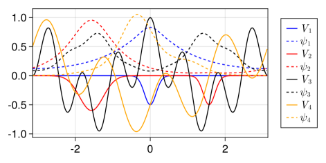
Figure 2. Potentials $V_{j}$, $j\in\{1,2,3,4\}$ together with the ground states $\psi_{j}$ of $H^{0}+V_{j}$.

Before starting the presentation of the numerical results, let us quickly remind the definitions of the three smallness parameters

$$\delta_{\text{\boldmath$\alpha$},\text{\boldmath$G$}}=\underset{\begin{subarray}{c}1\leqslant i,j\leqslant n\end{subarray}}{\text{{max}}}\;\sqrt{|\alpha_{i}\alpha_{j}|}\left|\!\left|G_{i}-G_{j}\right|\!\right|_{a},\qquad\delta_{\text{\boldmath$\alpha$}}=\left|1-\sum_{j=1}^{n}\alpha_{j}\right|,\qquad\delta_{g}=\left|\!\left|g\right|\!\right|_{a},$$

with $g=G-\sum_{j=1}^{n}\alpha_{j}G_{j}$.

5.1. Choice of closest $G_{j}$ for standard perturbation theory

When there are several $G_{j}$’s, standard perturbation theory approximates $\mathcal{F}(G)$ by using only one of those $G_{j}$’s for $j\in\{1,\dots,n\}$, so we need a way to choose it. Since there is a priori no way to know which one is going to provide the best approximation, a possible simple choice is to take $G_{j}$ with

$$j=\underset{\begin{subarray}{c}1\leqslant i\leqslant n\end{subarray}}{\text{{argmin}}}\quad\left|\!\left|G-G_{i}\right|\!\right|_{e}.$$ (21)

This choice leads to singularities in plots, because the index $j$ can change non-smoothly as we change the parameters $\alpha$ in the definition of $G$. The standard perturbation theory approximation of order $\ell$ using $G_{j}$ is then

$$\mathbb{P}^{j}_{\ell}:=\sum_{p=0}^{\ell}\mathcal{P}_{p}^{j},$$

where $\mathcal{P}_{p}^{j}$ is as in (12) but with the index $1$ replaced by $j$. By fairness, as a choice of $j$ we took

$$j_{\ell}=\underset{\begin{subarray}{c}1\leqslant i\leqslant n\end{subarray}}{\text{{argmin}}}\quad\left|\!\left|\mathcal{F}\left(G_{i}\right)-\mathbb{P}^{i}_{\ell}\right|\!\right|_{e},$$ (22)

which is the best one that standard perturbation theory provides, for each $\ell$, and provides continuous density matrices as well as $\mathbb{P}^{j}_{\ell}$ as parameters change.

5.2. Multipoint approximation when ${\delta_{g}=0}$ and $\delta_{\text{\boldmath$\alpha$},\text{\boldmath$G$}}\rightarrow 0$

We study the behaviour of the multipoint approximation as $G\in\operatorname{Aff}\left(G_{j}\right)_{j=1}^{n}$ and as $G_{j}\rightarrow G_{1}$ for all $j\in\{2,\dots,n\}$. More precisely, we take $n=4$, $\text{\boldmath$\alpha$}=\left(-0.3,0.4,0.3,0.6\right)$, and

$$G_{1}:=V_{1},\qquad G_{j}:=V_{1}+\varepsilon V_{j},\qquad j\in\{2,3,4\}$$

and $G:=\sum_{j=1}^{n}\alpha_{j}G_{j}$. Then, as $\varepsilon\rightarrow 0$, we have $\delta_{\text{\boldmath$\alpha$},\text{\boldmath$G$}}=c\varepsilon$ for some $c>0$ independent of $\varepsilon$. In Figure 3, we display the error $D_{e}\left(\mathcal{F}_{\text{exact}},\mathcal{F}_{\text{approx}}\right)$ between the exact density matrix

$$\mathcal{F}_{\text{exact}}:=\mathcal{F}\left(\sum_{j=1}^{n}\alpha_{j}G_{j}\right)$$

and several approximating quantities $\mathcal{F}_{\text{approx}}$, i.e., the zeroth and first order of multipoint perturbation, as well as the zeroth, first, second and third orders of standard perturbation theory given in (12) for comparison. The numerical results are displayed on Figure 3, where we simulate two different cases, namely $\delta_{\text{\boldmath$\alpha$}}=0$ on the left and $\delta_{\text{\boldmath$\alpha$}}>0$ on the right.

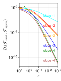
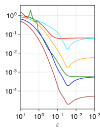
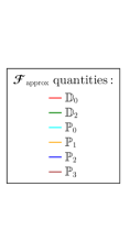
Figure 3. Comparision of the exact solution $\mathcal{F}_{\text{exact}}$ with the approximations $\mathcal{F}_{\text{approx}}$ based on multipoint perturbation theory (3.3) and based on standard perturbation theory (12). (Left) $\text{\boldmath$\alpha$}=(-0.3,0.4,0.3,0.6)$ so that ${s_{\text{\boldmath$\alpha$}}=1}$. The slopes of the asymptotic curves are indicated with the same color as the plot. (Right) $\text{\boldmath$\alpha$}=(-0.4,0.5,0.4,0.7)$ so ${s_{\text{\boldmath$\alpha$}}=1.2\neq 1}$.

As expected by the theoretical results presented in Section 3.4, we observe that the orders of convergence for the perturbative expansion are the expected ones, in particular the linear approximation of $\mathcal{F}$ (i.e. $\mathbb{D}_{0}$) which corresponds to the zeroth expansion order in the multipoint perturbation theory is asymptotically of same accuracy as the first expansion order in standard perturbation theory when $\delta_{\text{\boldmath$\alpha$},\text{\boldmath$G$}}\rightarrow 0$. Comparing the slopes of the error plots, we observe that the bound (16) is sharp in the case $\delta_{\text{\boldmath$\alpha$}}=0$.

5.3. Multipoint approximation when $\delta_{g}=0$, $\delta_{\text{\boldmath$\alpha$}}\neq 0$ and $\left(G_{j}\right)_{j=1}^{n}$ constant

We now consider $G$ as a linear combination of the $G_{j}$’s but not necessarily an affine one, i.e. the sum of $\alpha_{j}$’s can be different from one. For this purpose, take

$$G_{1}:=V_{1},\qquad G_{2}:=V_{1}+\frac{V_{2}}{5}.$$

In this situation, we show in Figure 4 the errors between the exact density matrix $\mathcal{F}(\alpha_{1}G_{1}+\alpha_{2}G_{2})$ and approximation thereof using standard perturbation theory and multipoint perturbation theory while $\text{\boldmath$\alpha$}=(\alpha_{1},\alpha_{2})$ changes. As expected, we mainly observe that multipoint perturbation is more efficient than standard perturbation on the neighborhood of $\operatorname{Aff}\left(G_{1},G_{2}\right)$ which is indicated by the dotted line and corresponds to the case $\alpha_{1}+\alpha_{2}=1$, when we compare approximations of similar orders. More precisely, the error with $\mathbb{D}_{0}$ as the approximation is smaller than the error with $\mathbb{P}_{0}$ and the error with $\mathbb{D}_{2}$ is smaller than the error with $\mathbb{P}_{2}$ around $\operatorname{Aff}\left(G_{1},G_{2}\right)$.

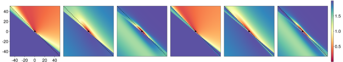
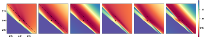
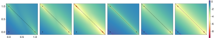
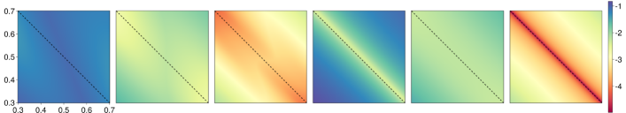
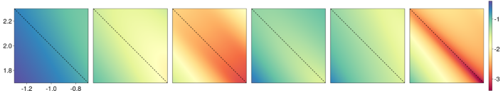
Figure 4. Error ${E(\mathcal{F}_{\text{approx}}):=D_{e}\left(\mathcal{F}_{\text{exact}},\mathcal{F}_{\text{approx}}\right)}$, the $x$-axis is $\alpha_{1}$ and the $y$-axis is $\alpha_{2}$, forming $\text{\boldmath$\alpha$}=\left(\alpha_{1},\alpha_{2}\right)$. From left to right, the quantities $\mathcal{F}_{\text{approx}}$ are respectively $\mathbb{P}_{0}$, $\mathbb{P}_{1}$, $\mathbb{P}_{2}$, $\mathbb{D}_{0}$, $\mathbb{D}_{1}$ and $\mathbb{D}_{2}$ as indicated on top. From top to bottom, we vary the range of $\alpha_{1}$ and $\alpha_{2}$, which is indicated on the left figure for each row. The two first rows indicate $E(\mathcal{F}_{\text{approx}})$ while the three last ones draw $\log_{10}E(\mathcal{F}_{\text{approx}})$. On the right of each row, we have the scale giving the correspondency between colors and values. We plot the particular points $\alpha$ equal to $(0,0)$, $(0,1)$ and $(1,0)$, and we plot the line $\alpha_{1}+\alpha_{2}=1$ with a dotted line.

5.4. Multipoint approximation when $\delta_{g}=0$, $\delta_{\text{\boldmath$\alpha$}}\rightarrow 0$ and $\left(G_{j}\right)_{j=1}^{n}$ constant.

We take the exact same situation as previously in Section 5.3, that is

$$G_{1}:=V_{1},\qquad G_{2}:=V_{1}+\frac{V_{2}}{5}.$$

and study the limit $\delta_{\text{\boldmath$\alpha$}}\rightarrow 0$. We take $\text{\boldmath$\alpha$}:=\left(\frac{1}{2}+\varepsilon,\frac{1}{2}+\varepsilon\right)$ and display in Figure 5 the relative errors $D_{e}\left(\mathcal{F}_{\text{exact}},\mathcal{F}_{\text{approx}}\right)$ against $\varepsilon\rightarrow 0$. This corresponds to a zoom of Figure 4 around the affine space at $(0.5,0.5)$ along the diagonal $\alpha_{1}=\alpha_{2}$.

Further, the plateau signifies the regime where the error in $\delta_{\text{\boldmath$\alpha$},\text{\boldmath$G$}}$ (i.e. $\delta_{\text{\boldmath$\alpha$},\text{\boldmath$G$}}^{\ell+1+\xi_{\ell}}$) dominates the one introduced by $\delta_{\text{\boldmath$\alpha$}}$ (i.e. $\delta_{\text{\boldmath$\alpha$}}^{\ell+1}$). We observe that when $\varepsilon$ is small enough (about $10^{-2}$), the error for the approximations based on multipoint perturbation are about one order of magnitude smaller than the errors for the approximations of similar approximation order using the standard perturbation method.

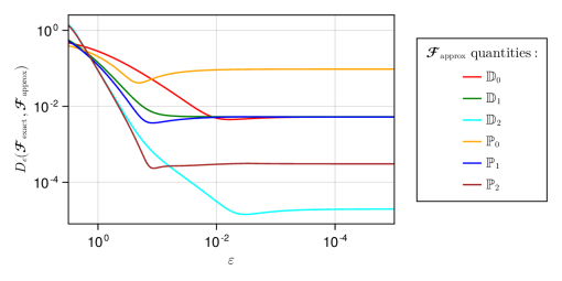
Figure 5. Relative errors $D_{e}\left(\mathcal{F}_{\text{exact}},\mathcal{F}_{\text{approx}}\right)$ with $\mathcal{F}_{\text{approx}}$ taken as $\mathbb{D}_{0},\mathbb{D}_{1},\mathbb{D}_{2},\mathbb{P}_{0},\mathbb{P}_{1},\mathbb{P}_{2}$ as $\delta_{\text{\boldmath$\alpha$}}\rightarrow 0$, when $\delta_{g}=0$ and $(G_{1},G_{2})$ is constant. We parametrize $\text{\boldmath$\alpha$}=\left(\frac{1}{2}+\varepsilon,\frac{1}{2}+\varepsilon\right)$.

5.5. Multipoint approximation when $\delta_{g}\rightarrow 0$, with $\left(G_{j}\right)_{j=1}^{n}$ constant

Let us take $n=2$,

$$G_{1}:=V_{1},\qquad G_{2}:=V_{1}+\frac{V_{2}}{5},\qquad\widetilde{G}_{3}:=V_{1}+\frac{V_{3}}{5},$$

and for $(\beta_{1},\beta_{2})\in\mathbb{R}^{2}$, define $G:=\beta_{1}G_{1}+\beta_{2}G_{2}+\varepsilon\widetilde{G}_{3}$, where $\varepsilon$ is going to converge to zero. Originally, one only knows $G$ and $G_{j}$, one does not know how $G$ was built, so we need to choose a way of finding $\text{\boldmath$\alpha$}=\left(\alpha_{j}\right)_{j=1}^{2}$ to then build $g:=G-\sum_{j=1}^{2}\alpha_{j}G_{j}$ and use the multipoint perturbation formula via the expansion in the $\mathbb{D}_{\ell}$’s. We consider three different ways of doing so. First, we consider the minimization problem

$$\underset{\begin{subarray}{c}\text{\boldmath$\alpha$}\in\mathbb{R}^{2}\end{subarray}}{\text{{min}}}\quad\left(D_{a}\left(G,\textstyle\sum_{j=1}^{2}\alpha_{j}G_{j}\right)^{2}+\xi\left|1-\textstyle\sum_{j=1}^{2}\alpha_{j}\right|^{2}\right),$$ (23)

and our three different ways of finding $\alpha$ will correspond to the optimizers of (23) with $\xi\in\{0,1,+\infty\}$. With an abuse of notation, the case $\xi=+\infty$ will refer to the problem

$$\underset{\begin{subarray}{c}\text{\boldmath$\alpha$}\in\mathbb{R}^{2}\\ \sum_{j=1}^{n}\alpha_{j}=1\end{subarray}}{\text{{min}}}\quad D_{a}\left(G,\textstyle\sum_{j=1}^{2}\alpha_{j}G_{j}\right)^{2}.$$

In Figure 6, we plot the relative error quantities $D_{e}\left(\mathcal{F}_{\text{exact}},\mathcal{F}_{\text{approx}}\right)$ against $\varepsilon$, resulting in $\delta_{g}\rightarrow 0$, for the three values of $\xi$, and for two values of $(\beta_{1},\beta_{2})$, one for which $\beta_{1}+\beta_{2}\neq 1$ and the other one respecting $\beta_{1}+\beta_{2}=1$. It seems that in any case, the best choice for $\xi$ is $0$.

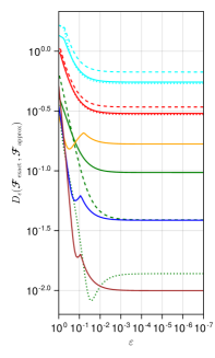
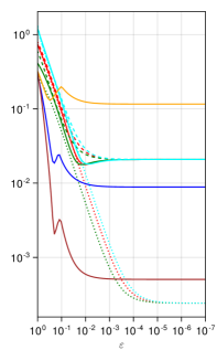
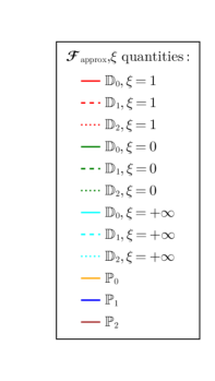
Figure 6. Relative errors against the parameter $\varepsilon$. We study here the convergence ${\delta_{g}\rightarrow 0}$, with $\beta$ and $\left(G_{j}\right)_{j=1}^{2}$ constant, and three ways of finding $\alpha$. (Left) $(\beta_{1},\beta_{2})=\left(0.3,1.2\right)$. (Right) $(\beta_{1},\beta_{2})=\left(0.3,0.7\right)$.

5.6. First multipoint approximation, and then standard perturbation theory

Since multipoint perturbation is particularly efficient on $\operatorname{Aff}\left(G_{j}\right)_{j=1}^{n}$, it is natural in the case when $G\notin\operatorname{Aff}\left(G_{j}\right)_{j=1}^{n}$ to try to first solve (23), then compute $\mathbb{D}_{2}$, and finally compute the second order approximation using standard perturbation theory between $\sum_{j=1}^{n}\alpha_{j}G_{j}$ and $G$. We observe that the resulting total error is very similar the last column in Figure 4, and thus omit to report the results here.

6. Proofs

In this section we provide the proofs of the propositions.

6.1. Bounds

Let us first start by showing a standard result, enabling to have a bound on $\left(z-H(G)\right)^{-1}$ explicit in $z$, and relating the bound to the definition (1) of $\mathcal{G}$.

Lemma 6.1 (Explicit bound on the resolvent).

Take an essentially self-adjoint and bounded from below operator $H^{0}$ on the Hilbert space $\mathcal{H}$. Take $G\in\mathcal{G}$, $\mu,\eta>1$ with $\eta$ large enough so that

$$\left|\!\left|\left(H^{0}+\eta\right)^{-\frac{1}{2}}G\left(H^{0}+\eta\right)^{-\frac{1}{2}}\right|\!\right|\leqslant\frac{1}{2}.$$ (24)

The last condition is satisfied for instance for $\eta=\max(4c^{G}_{1/8},1)$, where $c^{G}_{\varepsilon}$ is defined in (1). Take a contour $\mathcal{C}\subset\mathbb{C}$ such that ${\rm d}\left(\mathcal{C},\sigma(H(G))\right)=:\xi>0$. Then there holds

$$\underset{\begin{subarray}{c}z\in\mathcal{C}\end{subarray}}{\text{{max}}}\;\left|\!\left|\left(z-H(G)\right)^{-1}\right|\!\right|_{e}\\ \leqslant 2\left(1+\frac{\left|\mu-\eta\right|}{\eta+\min\sigma(H(G))}\right)\left(1+2\left|\eta+\underset{\begin{subarray}{c}z\in\mathcal{C}\end{subarray}}{\text{{max}}}\;\left|z\right|\right|\left(1+\frac{\left|\eta+\underset{\begin{subarray}{c}z\in\mathcal{C}\end{subarray}}{\text{{max}}}\;\left|z\right|\right|}{\xi}\right)\right).$$ (25)

We used the notation ${\rm d}\left(S_{1},S_{2}\right):=\min_{s_{1}\in S_{1},s_{2}\in S_{2}}\left|s_{1}-s_{2}\right|$, and the energy norm which depends on $\mu$ is defined in (4).

Proof of Lemma 6.1.

We denote by $\lambda:=\min\sigma(H^{0})\geqslant 0$. Also define

$$D :=\left(H^{0}+\eta\right)^{\frac{1}{2}}\left(H(G)+\eta\right)^{-1}\left(H^{0}+\eta\right)^{\frac{1}{2}},$$

$$J :=\left(H^{0}+\eta\right)^{-\frac{1}{2}}G\left(H^{0}+\eta\right)^{-\frac{1}{2}},$$

and there holds $\left|\!\left|J\right|\!\right|\leqslant\frac{1}{2}$ by assumption (24). In the sense of forms, $1\leqslant\eta\leqslant H^{0}+\eta$, so $\left|\!\left|\left(H^{0}+\eta\right)^{-\frac{1}{2}}\right|\!\right|\leqslant 1$. Moreover

$$D^{-1}=\left(H^{0}+\eta\right)^{-\frac{1}{2}}\left(H(G)+\eta\right)\left(H^{0}+\eta\right)^{-\frac{1}{2}}=1+J$$

and hence $\left|\!\left|D\right|\!\right|\leqslant\left(1-\left|\!\left|J\right|\!\right|\right)^{-1}\leqslant 2$. Now

$$\left(H^{0}+\eta\right)^{\frac{1}{2}}\left(H(G)-z\right)^{-1}\left(H^{0}+\eta\right)^{\frac{1}{2}}$$

$$\qquad=\left(H^{0}+\eta\right)^{\frac{1}{2}}\left(H(G)+\eta\right)^{-1}\left(H(G)+\eta\right)\left(H(G)-z\right)^{-1}\left(H^{0}+\eta\right)^{\frac{1}{2}}$$

$$\qquad=D\left(H^{0}+\eta\right)^{-\frac{1}{2}}\left(H(G)+\eta\right)\left(H(G)-z\right)^{-1}\left(H^{0}+\eta\right)^{\frac{1}{2}}$$

$$\qquad=D\left(1+\left(\eta+z\right)\left(H^{0}+\eta\right)^{-\frac{1}{2}}\left(H(G)-z\right)^{-1}\left(H^{0}+\eta\right)^{\frac{1}{2}}\right)$$

$$\qquad=D\left(1+\left(\eta+z\right)\left(H^{0}+\eta\right)^{-\frac{1}{2}}\left(1+\left(\eta+z\right)\left(H(G)-z\right)^{-1}\right)\left(H^{0}+\eta\right)^{-\frac{1}{2}}D\right),$$

and we deduce that

$$\left|\!\left|\left(H^{0}+\eta\right)^{\frac{1}{2}}\left(H(G)-z\right)^{-1}\left(H^{0}+\eta\right)^{\frac{1}{2}}\right|\!\right|\leqslant 2\left(1+2\left|\eta+z\right|\left(1+\frac{\left|\eta+z\right|}{{\rm d}\left(z,\sigma\left(H(G)\right)\right)}\right)\right).$$

Then

$$\left(H^{0}+\mu\right)\left(H^{0}+\eta\right)^{-1}=1+\left(\mu-\eta\right)\left(H^{0}+\eta\right)^{-1}$$

so

$$\left|\!\left|\left(H^{0}+\mu\right)\left(H^{0}+\eta\right)^{-1}\right|\!\right|\leqslant 1+\frac{\left|\mu-\eta\right|}{\lambda+\eta}.$$

We have $H^{0}+\mu\geqslant 1$ and $\left(H^{0}+\eta\right)^{-1}\geqslant 0$ in the sense of forms, so $\left(H^{0}+\mu\right)\left(H^{0}+\eta\right)^{-1}\geqslant 0$. By monotonicity of the square root of operators, we deduce that

$$\left|\!\left|\left(\left(H^{0}+\mu\right)\left(H^{0}+\eta\right)^{-1}\right)^{\frac{1}{2}}\right|\!\right|\leqslant\left(1+\frac{\left|\mu-\eta\right|}{\lambda+\eta}\right)^{\frac{1}{2}}.$$

We deduce (25) by writting

$$\left(H^{0}+\mu\right)^{\frac{1}{2}}\left(H(G)-z\right)^{-1}\left(H^{0}+\mu\right)^{\frac{1}{2}}\\ =\sqrt{\left(H^{0}+\mu\right)\left(H^{0}+\eta\right)^{-1}}\left(H^{0}+\eta\right)^{\frac{1}{2}}\left(H(G)-z\right)^{-1}\left(H^{0}+\eta\right)^{\frac{1}{2}}\sqrt{\left(H^{0}+\mu\right)\left(H^{0}+\eta\right)^{-1}}.$$

We deduce that

$$\left|\!\left|\left(z-H(G)\right)^{-1}\right|\!\right|_{e}\leqslant 2\left(1+\frac{\left|\mu-\eta\right|}{\eta+\lambda}\right)\left(1+2\left|\eta+z\right|\left(1+\frac{\left|\eta+z\right|}{{\rm d}\left(z,\sigma\left(H(G)\right)\right)}\right)\right),$$

from which we easily get (25).

We then search for the more explicit condition $\eta=\max(4c^{G}_{1/8},1)$ that fulfills (24). Take $G\in\mathcal{G}$ and $\varphi\in\mathcal{H}$ such that the following expressions are finite, we have

$$\left|\!\left|\left|G\right|^{\frac{1}{2}}\left(H^{0}+\eta\right)^{-\frac{1}{2}}\varphi\right|\!\right|^{2}=\left<\left(H^{0}+\eta\right)^{-\frac{1}{2}}\varphi,\left|G\right|\left(H^{0}+\eta\right)^{-\frac{1}{2}}\varphi\right>$$

$$\qquad\underset{\begin{subarray}{c}~{}\eqref{eq:set_operators}\end{subarray}}{\leqslant}\;\left<\left(H^{0}+\eta\right)^{-\frac{1}{2}}\varphi,\left(\varepsilon H^{0}+c^{G}_{\varepsilon}\right)\left(H^{0}+\eta\right)^{-\frac{1}{2}}\varphi\right>$$

$$\qquad=\left<\varphi,\left(\varepsilon+\frac{c^{G}_{\varepsilon}-\varepsilon\eta}{H^{0}+\eta}\right)\varphi\right>\leqslant\left(\varepsilon+\frac{\left|c^{G}_{\varepsilon}-\varepsilon\eta\right|}{\lambda+\eta}\right)\left|\!\left|\varphi\right|\!\right|^{2}$$

$$\qquad\leqslant\left(2\varepsilon+\frac{c^{G}_{\varepsilon}}{\lambda+\eta}\right)\left|\!\left|\varphi\right|\!\right|^{2}\leqslant\left(2\varepsilon+\frac{c^{G}_{\varepsilon}}{\eta}\right)\left|\!\left|\varphi\right|\!\right|^{2},$$

so by the polar decomposition $G=\left|G\right|U$,

$$\left|\!\left|\left(H^{0}+\eta\right)^{-\frac{1}{2}}G\left(H^{0}+\eta\right)^{-\frac{1}{2}}\right|\!\right|=\left|\!\left|\left(H^{0}+\eta\right)^{-\frac{1}{2}}\left|G\right|^{\frac{1}{2}}U\left|G\right|^{\frac{1}{2}}\left(H^{0}+\eta\right)^{-\frac{1}{2}}\right|\!\right|$$

$$\qquad\leqslant\left|\!\left|\left|G\right|^{\frac{1}{2}}\left(H^{0}+\eta\right)^{-\frac{1}{2}}\right|\!\right|^{2}\left|\!\left|U\right|\!\right|\leqslant 2\varepsilon+\frac{c^{G}_{\varepsilon}}{\eta}.$$

Choosing $\varepsilon=1/8$ and $\eta$ such that $\frac{c^{G}_{1/8}}{\eta}\leqslant 1/4$ guaranties that (24) is satisfied. ∎

6.2. Standard perturbation theory

We then provide a proof of the standard perturbation result.

Proof of Proposition 2.2.

We remark that

$$\left(H^{0}+\mu\right)^{\frac{\kappa}{2}}\left(z-H(G)\right)^{-1}\left(H^{0}+\mu\right)^{\frac{\kappa}{2}}$$

$$\qquad=\left(H^{0}+\mu\right)^{\frac{\kappa}{2}}\left(z-H(G_{1})\right)^{-1}\left(H^{0}+\mu\right)^{\frac{\kappa}{2}}$$

$$\qquad\qquad\times\left(H^{0}+\mu\right)^{-\frac{\kappa}{2}}\left(1-g\left(z-H(G_{1})\right)^{-1}\right)^{-1}\left(H^{0}+\mu\right)^{\frac{\kappa}{2}}$$

$$\qquad=\left(H^{0}+\mu\right)^{\frac{\kappa}{2}}\left(z-H(G_{1})\right)^{-1}\left(H^{0}+\mu\right)^{\frac{\kappa}{2}}$$

$$\qquad\qquad\times\left(1-\left(H^{0}+\mu\right)^{-\frac{\kappa}{2}}g\left(H^{0}+\mu\right)^{-\frac{\kappa}{2}}\left(H^{0}+\mu\right)^{\frac{\kappa}{2}}\left(z-H(G_{1})\right)^{-1}\left(H^{0}+\mu\right)^{\frac{\kappa}{2}}\right)^{-1}.$$ (26)

Provided that the condition $\left|\!\left|g\right|\!\right|_{a}\leqslant 1/(2C)$ is satisfied, (10) is well-defined in the corresponding norms and we have

$$\left|\!\left|\left(z-H(G)\right)^{-1}\right|\!\right|_{e}\leqslant\frac{\left|\!\left|\left(z-H(G_{1})\right)^{-1}\right|\!\right|_{e}}{1-\left|\!\left|g\right|\!\right|_{a}\left|\!\left|\left(z-H(G_{1})\right)^{-1}\right|\!\right|_{e}}\leqslant 2C.$$

We can then make a Neumann expansion and have

$$\left(z-H(G)\right)^{-1}-\left(z-H(G_{1})\right)^{-1}\sum_{p=0}^{\ell}\left(g\left(z-H(G_{1})\right)^{-1}\right)^{p}$$

$$\qquad\qquad=\left(z-H(G_{1})\right)^{-1}\sum_{p=\ell+1}^{+\infty}\left(g\left(z-H(G_{1})\right)^{-1}\right)^{p}$$

$$\qquad\qquad=\left(z-H(G_{1})\right)^{-1}\left(g\left(z-H(G_{1})\right)^{-1}\right)^{\ell+1}\left(1-g\left(z-H(G_{1})\right)^{-1}\right)^{-1}$$

and we obtain

$$\left|\!\left|\left(z-H(G)\right)^{-1}-\left(z-H(G_{1})\right)^{-1}\sum_{p=0}^{\ell}\left(g\left(z-H(G_{1})\right)^{-1}\right)^{p}\right|\!\right|_{e}\\ \leqslant\left|\!\left|g\right|\!\right|_{a}^{\ell+1}\frac{\left|\!\left|\left(z-H(G_{1})\right)^{-1}\right|\!\right|_{e}^{\ell+2}}{1-\left|\!\left|g\right|\!\right|_{a}\left|\!\left|\left(z-H(G_{1})\right)^{-1}\right|\!\right|_{e}}\leqslant 2C^{\ell+2}\left|\!\left|g\right|\!\right|_{a}^{\ell+1}.$$

Still in series of $g$, by integration over $\mathcal{C}$ and using Cauchy’s formula (6), we can deduce the expansion

$$\mathcal{F}(G)=\sum_{m=0}^{+\infty}\mathcal{P}_{m}.$$

We integrate over $z\in\mathcal{C}$ and obtain the result (11). ∎

6.3. Main formula

We will use the notation $R_{j}:=\left(z-H(G_{j})\right)^{-1}$, $G_{ij}:=G_{i}-G_{j}$ so we have, by the resolvent formula,

$$\left(z-H(G)\right)^{-1}-R_{j}=\left(z-H(G)\right)^{-1}(G-G_{j})R_{j},\qquad\qquad R_{j}-R_{i}=R_{j}G_{ji}R_{i}.$$ (27)

Proof of Theorem 3.1.

For any ${\bm{\alpha}}=(\alpha_{i})_{i=1}^{n}\in\mathbb{R}^{n},$ let $s_{\text{\boldmath$\alpha$}}:=\sum_{j=1}^{n}\alpha_{j}$. There holds

$$s_{\text{\boldmath$\alpha$}}\left(1-\left(z-H(G)\right)\mathbb{L}_{z}\right) =\left(z-H(G)\right)\left(\left(\sum_{j=1}^{n}\alpha_{j}\right)\left(z-H(G)\right)^{-1}-\sum_{j=1}^{n}\alpha_{j}R_{j}\right)$$

$$=\left(z-H(G)\right)\sum_{j=1}^{n}\alpha_{j}\left(\left(z-H(G)\right)^{-1}-R_{j}\right).$$

Using (27), and recalling that $g:=G-\sum_{j=1}^{n}\alpha_{j}G_{j}$, we obtain

$$s_{\text{\boldmath$\alpha$}}\left(1-\left(z-H(G)\right)\mathbb{L}_{z}\right) =\sum_{j=1}^{n}\alpha_{j}\left(G-G_{j}\right)R_{j}$$

$$=g\sum_{j=1}^{n}\alpha_{j}R_{j}+\sum_{j=1}^{n}\alpha_{j}\left(\left(\sum_{i=1}^{n}\alpha_{i}G_{i}\right)-G_{j}\right)R_{j}$$

$$=g\sum_{j=1}^{n}\alpha_{j}R_{j}+\sum_{i,j=1}^{n}\alpha_{j}\alpha_{i}\left(G_{i}-G_{j}\right)R_{j}+\left(s_{\text{\boldmath$\alpha$}}-1\right)\sum_{j=1}^{n}\alpha_{j}G_{j}R_{j}$$

$$=s_{\text{\boldmath$\alpha$}}g\mathbb{L}_{z}+\sum_{i,j=1}^{n}\alpha_{j}\alpha_{i}\left(G_{i}-G_{j}\right)R_{j}+\left(s_{\text{\boldmath$\alpha$}}-1\right)s_{\text{\boldmath$\alpha$}}\mathbb{A}_{z}.$$

Noting that $G_{ji}=-G_{ij}$, we rearrange the second term on the right-hand side into

$$\sum_{\begin{subarray}{c}1\leqslant i,j\leqslant n\end{subarray}}\alpha_{i}\alpha_{j}G_{ij}R_{j} =\frac{1}{2}\sum_{\begin{subarray}{c}1\leqslant i,j\leqslant n\end{subarray}}\alpha_{i}\alpha_{j}G_{ij}R_{j}+\frac{1}{2}\sum_{\begin{subarray}{c}1\leqslant i,j\leqslant n\end{subarray}}\alpha_{j}\alpha_{i}G_{ji}R_{i}$$

$$=\frac{1}{2}\sum_{\begin{subarray}{c}1\leqslant i,j\leqslant n\end{subarray}}\alpha_{i}\alpha_{j}G_{ij}\left(R_{j}-R_{i}\right).$$

Using again (27), we get

$$\sum_{\begin{subarray}{c}1\leqslant i,j\leqslant n\end{subarray}}\alpha_{i}\alpha_{j}G_{ij}R_{j} =-\frac{1}{2}\sum_{\begin{subarray}{c}1\leqslant i,j\leqslant n\end{subarray}}\alpha_{i}\alpha_{j}G_{ij}R_{j}G_{ij}R_{i}$$

$$=-\sum_{\begin{subarray}{c}1\leqslant i<j\leqslant n\end{subarray}}\alpha_{i}\alpha_{j}G_{ij}R_{j}G_{ij}R_{i}$$

$$=-s_{\text{\boldmath$\alpha$}}\mathbb{H}_{z}.$$

Therefore,

$$\left(1-\left(z-H(G)\right)\mathbb{L}_{z}\right)=g\mathbb{L}_{z}-\mathbb{H}_{z}+(s_{\text{\boldmath$\alpha$}}-1)\mathbb{A}_{z},$$

which is equivalent to

$$\left(z-H(G)\right)^{-1}(1+\mathbb{H}_{z}+(1-s_{\text{\boldmath$\alpha$}})\mathbb{A}_{z}-g\mathbb{L}_{z})=\mathbb{L}_{z}.$$

∎

6.4. Multipoint perturbation theory bound

Proof of Corollary 3.6.

We have

$$\left(H^{0}+\mu\right)^{-\frac{\kappa}{2}}\mathbb{H}_{z}\left(H^{0}+\mu\right)^{\frac{\kappa}{2}} =s_{\text{\boldmath$\alpha$}}^{-1}\sum_{\begin{subarray}{c}1\leqslant i<j\leqslant n\end{subarray}}\alpha_{i}\alpha_{j}\left(H^{0}+\mu\right)^{-\frac{\kappa}{2}}G_{ij}R_{j}G_{ij}R_{i}\left(H^{0}+\mu\right)^{\frac{\kappa}{2}}$$

$$=s_{\text{\boldmath$\alpha$}}^{-1}\sum_{\begin{subarray}{c}1\leqslant i<j\leqslant n\end{subarray}}\alpha_{i}\alpha_{j}\left(H^{0}+\mu\right)^{-\frac{\kappa}{2}}G_{ij}\left(H^{0}+\mu\right)^{-\frac{\kappa}{2}}$$

$$\quad\times\left(H^{0}+\mu\right)^{\frac{\kappa}{2}}R_{j}\left(H^{0}+\mu\right)^{\frac{\kappa}{2}}\left(H^{0}+\mu\right)^{-\frac{\kappa}{2}}G_{ij}\left(H^{0}+\mu\right)^{-\frac{\kappa}{2}}$$

$$\quad\times\left(H^{0}+\mu\right)^{\frac{\kappa}{2}}R_{i}\left(H^{0}+\mu\right)^{\frac{\kappa}{2}}.$$

Recalling that $\delta_{\text{\boldmath$\alpha$},\text{\boldmath$G$}}:=\underset{\begin{subarray}{c}1\leqslant i,j\leqslant n\end{subarray}}{\text{{max}}}\;\sqrt{|\alpha_{i}\alpha_{j}|}\left|\!\left|G_{ij}\right|\!\right|_{a}$, we obtain

$$\left|\!\left|\left(H^{0}+\mu\right)^{-\frac{\kappa}{2}}\mathbb{H}_{z}\left(H^{0}+\mu\right)^{\frac{\kappa}{2}}\right|\!\right|\leqslant\delta_{\text{\boldmath$\alpha$},\text{\boldmath$G$}}^{2}\tfrac{n(n-1)}{2}s_{\text{\boldmath$\alpha$}}^{-1}\underset{\begin{subarray}{c}1\leqslant j\leqslant n\\ z\in\mathcal{C}\end{subarray}}{\text{{max}}}\;\left|\!\left|R_{j}\right|\!\right|_{e}^{2}.$$

Similarly,

$$\left|\!\left|\left(H^{0}+\mu\right)^{-\frac{\kappa}{2}}\mathbb{A}_{z}\left(H^{0}+\mu\right)^{\frac{\kappa}{2}}\right|\!\right| \leqslant ns_{\text{\boldmath$\alpha$}}^{-1}\underset{\begin{subarray}{c}1\leqslant j\leqslant n\\ z\in\mathcal{C}\end{subarray}}{\text{{max}}}\;\left|\alpha_{j}\right|\left|\!\left|G_{j}\right|\!\right|_{a}\left|\!\left|R_{j}\right|\!\right|_{e}$$

$$\left|\!\left|\left(H^{0}+\mu\right)^{\frac{\kappa}{2}}\mathbb{L}_{z}\left(H^{0}+\mu\right)^{\frac{\kappa}{2}}\right|\!\right| \leqslant ns_{\text{\boldmath$\alpha$}}^{-1}\underset{\begin{subarray}{c}1\leqslant j\leqslant n\\ z\in\mathcal{C}\end{subarray}}{\text{{max}}}\;\left|\alpha_{j}\right|\left|\!\left|R_{j}\right|\!\right|_{e}.$$

Standard arguments, expressed in form of Lemma 6.1, enable us to bound $\left|\!\left|R_{j}\right|\!\right|_{e}$ using the definition of $\mathcal{G}$. Thus we have a more explicit bound on

$$\gamma :=ns_{\text{\boldmath$\alpha$}}^{-1}\underset{\begin{subarray}{c}1\leqslant j\leqslant n\\ z\in\mathcal{C}\end{subarray}}{\text{{max}}}\;\left(\left|\!\left|R_{j}\right|\!\right|_{e}\left[\left|\alpha_{j}\right|\left(1+\left|\!\left|G_{j}\right|\!\right|_{a}\right)+\tfrac{1}{2}(n-1)\left|\!\left|R_{j}\right|\!\right|_{e}\right]\right)\leqslant\beta c_{\text{\boldmath$\alpha$}},$$ (28)

where $\beta$ depends neither on $G$ nor on $\alpha$, and we obtain

$$\left|\!\left|\left(H^{0}+\mu\right)^{-\frac{\kappa}{2}}\mathbb{H}_{z}\left(H^{0}+\mu\right)^{\frac{\kappa}{2}}\right|\!\right| \leqslant\gamma\delta_{\text{\boldmath$\alpha$},\text{\boldmath$G$}}^{2},$$

$$\left|\!\left|\left(H^{0}+\mu\right)^{-\frac{\kappa}{2}}(1-s_{\text{\boldmath$\alpha$}})\mathbb{A}_{z}\left(H^{0}+\mu\right)^{\frac{\kappa}{2}}\right|\!\right| \leqslant\gamma\delta_{\text{\boldmath$\alpha$}},$$

$$\left|\!\left|\left(H^{0}+\mu\right)^{-\frac{\kappa}{2}}g\mathbb{L}_{z}\left(H^{0}+\mu\right)^{\frac{\kappa}{2}}\right|\!\right| \leqslant\gamma\delta_{g}.$$

Hence,

$$\left|\!\left|\left(H^{0}+\mu\right)^{-\frac{\kappa}{2}}\left(\mathbb{H}_{z}-(s_{\text{\boldmath$\alpha$}}-1)\mathbb{A}_{z}-g\mathbb{L}_{z}\right)\left(H^{0}+\mu\right)^{\frac{\kappa}{2}}\right|\!\right|\leqslant\gamma\left(\delta_{\text{\boldmath$\alpha$},\text{\boldmath$G$}}^{2}+\delta_{\text{\boldmath$\alpha$}}+\delta_{g}\right),$$

and assuming that $\delta_{\text{\boldmath$\alpha$},\text{\boldmath$G$}}^{2}+\delta_{\text{\boldmath$\alpha$}}+\delta_{g}<(2\gamma)^{-1}$, we can proceed to the Neumann expansion of $\left(1+\mathbb{H}_{z}-(s_{\text{\boldmath$\alpha$}}-1)\mathbb{A}_{z}-g\mathbb{L}_{z}\right)^{-1}$, and have

$$\left(1+\mathbb{H}_{z}-(s_{\text{\boldmath$\alpha$}}-1)\mathbb{A}_{z}-g\mathbb{L}_{z}\right)^{-1}=\sum_{p=0}^{+\infty}\left(-\mathbb{H}_{z}+(s_{\text{\boldmath$\alpha$}}-1)\mathbb{A}_{z}+g\mathbb{L}_{z}\right)^{p}.$$

Now, to obtain the corresponding series for $\mathcal{F}(G)$, we need to compute

$$\mathcal{F}(G) =\frac{1}{2\pi i}\oint_{\mathcal{C}}\left(z-H\left(G\right)\right)^{-1}{\rm d}z$$

$$=\frac{1}{2\pi i}\oint_{\mathcal{C}}\mathbb{L}_{z}\left(1+\mathbb{H}_{z}-(s_{\text{\boldmath$\alpha$}}-1)\mathbb{A}_{z}-g\mathbb{L}_{z}\right)^{-1}{\rm d}z$$

$$=\sum_{p=0}^{+\infty}\frac{1}{2\pi i}\oint_{\mathcal{C}}\mathbb{L}_{z}\left(-\mathbb{H}_{z}+(s_{\text{\boldmath$\alpha$}}-1)\mathbb{A}_{z}+g\mathbb{L}_{z}\right)^{p}{\rm d}z$$

$$=\sum_{p=0}^{+\infty}\widetilde{\mathcal{D}}_{p},$$

where

$$\widetilde{\mathcal{D}}_{(a,b,c)} :=\mathcal{D}_{(2a,b,c)},\qquad\qquad\widetilde{\mathcal{D}}_{p}:=\sum_{\begin{subarray}{c}a,b,c\in\mathbb{N}\\ a+b+c=p\end{subarray}}\widetilde{\mathcal{D}}_{(a,b,c)},\qquad\qquad\widetilde{\mathbb{D}}_{\ell}:=\sum_{p=0}^{\ell}\widetilde{\mathcal{D}}_{p}.$$

Remark 6.2.

We give here a bound which is not used in the following, but that we find interesting to present

$$\mathcal{F}(G)-\widetilde{\mathbb{D}}_{\ell}=\sum_{p=\ell+1}^{+\infty}\frac{1}{2\pi i}\oint_{\mathcal{C}}\mathbb{L}_{z}\left(-\mathbb{H}_{z}+(s_{\text{\boldmath$\alpha$}}-1)\mathbb{A}_{z}+g\mathbb{L}_{z}\right)^{p}{\rm d}z$$

so

$$\left(H^{0}+\mu\right)^{\frac{\kappa}{2}}\left(\mathcal{F}(G)-\widetilde{\mathbb{D}}_{\ell}\right)\left(H^{0}+\mu\right)^{\frac{\kappa}{2}}=\sum_{p=\ell+1}^{+\infty}\frac{1}{2\pi i}\oint_{\mathcal{C}}\left(H^{0}+\mu\right)^{\frac{\kappa}{2}}\mathbb{L}_{z}\left(H^{0}+\mu\right)^{\frac{\kappa}{2}}\\ \times\left(\left(H^{0}+\mu\right)^{-\frac{\kappa}{2}}\left(-\mathbb{H}_{z}+(s_{\text{\boldmath$\alpha$}}-1)\mathbb{A}_{z}+g\mathbb{L}_{z}\right)\left(H^{0}+\mu\right)^{\frac{\kappa}{2}}\right)^{p}{\rm d}z$$

and we can conclude that

$$\left|\!\left|\mathcal{F}(G)-\widetilde{\mathbb{D}}_{\ell}\right|\!\right|_{e}\leqslant c\left(\gamma\left(\delta_{\text{\boldmath$\alpha$},\text{\boldmath$G$}}^{2}+\delta_{\text{\boldmath$\alpha$}}+\delta_{g}\right)\right)^{\ell+1}=c\gamma^{\ell+1}\sum_{\begin{subarray}{c}a,b,c\in\mathbb{N}\\ a+b+c=\ell+1\end{subarray}}\delta_{\text{\boldmath$\alpha$},\text{\boldmath$G$}}^{2a}\delta_{\text{\boldmath$\alpha$}}^{b}\delta_{g}^{c}.$$

Now summing differently, and since $\mathcal{D}_{\left(2a+1,b,c\right)}=0$ for any $a,b,c\in\mathbb{N}$,

$$\mathcal{F}(G)=\sum_{p=0}^{+\infty}\widetilde{\mathcal{D}}_{p}=\sum_{p=0}^{+\infty}\mathcal{D}_{p},$$

so

$$\mathcal{F}(G)-\mathbb{D}_{\ell}=\sum_{p=\ell+1}^{+\infty}\mathcal{D}_{p}=\sum_{\begin{subarray}{c}a,b,c\in\mathbb{N}\\ a+b+c\geqslant\ell+1\end{subarray}}\mathcal{D}_{\left(a,b,c\right)},$$

but

$$\left|\!\left|\widetilde{\mathcal{D}}_{(a,b,c)}\right|\!\right|_{e}\leqslant c\delta_{\text{\boldmath$\alpha$},\text{\boldmath$G$}}^{2a}\delta_{\text{\boldmath$\alpha$}}^{b}\delta_{g}^{c},\qquad\qquad\left|\!\left|\mathcal{D}_{(a,b,c)}\right|\!\right|_{e}\leqslant c\delta_{a\in 2\mathbb{N}}\delta_{\text{\boldmath$\alpha$},\text{\boldmath$G$}}^{a}\delta_{\text{\boldmath$\alpha$}}^{b}\delta_{g}^{c},$$

where $c\leqslant C^{\prime}c_{\text{\boldmath$\alpha$}}^{m}$ for some $m\in\mathbb{N}$ and $C^{\prime}$ which does not depend on $G$ or $\alpha$. We conclude by summation, using

$$\left|\!\left|\mathcal{F}(G)-\mathbb{D}_{\ell}\right|\!\right|_{e}\leqslant C^{\prime}_{\ell}c_{\text{\boldmath$\alpha$}}^{m_{\ell}}\sum_{\begin{subarray}{c}a,b,c\in\mathbb{N}\\ a+b+c\geqslant\ell+1\end{subarray}}\delta_{a\in 2\mathbb{N}}\delta_{\text{\boldmath$\alpha$},\text{\boldmath$G$}}^{a}\delta_{\text{\boldmath$\alpha$}}^{b}\delta_{g}^{c}\leqslant C^{\prime}_{\ell}c_{\text{\boldmath$\alpha$}}^{m_{\ell}}\sum_{\begin{subarray}{c}a\in 2\mathbb{N}\\ b,c\in\mathbb{N}\\ a+b+c\in\{\ell+1,\ell+2\}\end{subarray}}\delta_{\text{\boldmath$\alpha$},\text{\boldmath$G$}}^{a+1}\delta_{\text{\boldmath$\alpha$}}^{b}\delta_{g}^{c}$$

as an intermediate step.

Let us now treat the case where $1/2>(2\gamma)^{-1}$ and

$$(2\gamma)^{-1}\leqslant\delta_{\text{\boldmath$\alpha$},\text{\boldmath$G$}}^{2}+\delta_{\text{\boldmath$\alpha$}}+\delta_{g}\leqslant 1/2,$$

so we also have that

$$q_{0}\leqslant\delta_{\text{\boldmath$\alpha$},\text{\boldmath$G$}}^{\ell+1+\xi_{\ell}}+\delta_{\text{\boldmath$\alpha$}}^{\ell+1}+\delta_{g}^{\ell+1},$$

for some $q_{0}>0$ independent of $\alpha$ and $g$. The bound remains true, but the preconstant $C_{\ell}$ may need to be increased, we detail here how we can provide a very coarse one. In this case $\delta_{g}\leqslant 1/2$ and $\delta_{\text{\boldmath$\alpha$}}\leqslant 1/2$, $c_{\alpha}$ is bounded from below uniformly in $\alpha$, i.e. $c_{\alpha}\geqslant q_{1}>0$, and for instance we can take $m_{\ell}=1$ and

$$\underset{\begin{subarray}{c}G\in\mathcal{G}\\ \delta_{g}\leqslant 1/2\end{subarray}}{\text{{max}}}\;\frac{\left|\!\left|\mathcal{F}(G)-\mathbb{D}_{\ell}\right|\!\right|_{e}}{c_{\text{\boldmath$\alpha$}}\left(\delta_{\text{\boldmath$\alpha$},\text{\boldmath$G$}}^{\ell+1+\xi_{\ell}}+\delta_{\text{\boldmath$\alpha$}}^{\ell+1}+\delta_{g}^{\ell+1}\right)}\leqslant\frac{1}{q_{0}q_{1}}\underset{\begin{subarray}{c}G\in\mathcal{G}\\ \delta_{g}\leqslant 1/2\end{subarray}}{\text{{max}}}\;\left|\!\left|\mathcal{F}(G)-\mathbb{D}_{\ell}\right|\!\right|_{e}=:C_{\ell},$$

this quantity being finite. This concludes the proof. ∎

6.5. Proof of Proposition 4.1

Proof of Proposition 4.1.

For any $a\in\{1,\dots,n\}$, any $z\in\left(\mathbb{C}\backslash\sigma(H(G_{a}))\right)\cup\{\lambda^{k}(G_{a})\}$, we define

$$R^{\perp}_{a}(z):=\left\{\begin{array}[]{ll}\left(\left(z-H(G_{a})\right)_{\mkern 1.0mu\vrule height=6.02777pt\mkern 2.0mu\left(\operatorname{Ker}\left(\lambda^{k}(G_{a})-H(G_{a})\right)\right)^{\perp}}\right)^{-1}&\mbox{on }\left(\operatorname{Ker}\left(\lambda^{k}(G_{a})-H(G_{a})\right)\right)^{\perp},\\ 0&\mbox{on }\operatorname{Ker}\left(\lambda^{k}(G_{a})-H(G_{a})\right),\end{array}\right.$$

extended on all of $\mathcal{H}$ by linearity. As a function of $z$, it is holomorphic in a neighborhood of $\{\lambda^{k}(G_{a})\}$ containing $\lambda^{k}(G_{a})$, and note that $R_{a}^{\perp}(\lambda^{k}(G_{j}))=K_{ja}$. Take $a\in\{1,\dots,n\}$, we define $P_{a}^{\perp}=1-P_{a}$ so for any $z\in\mathbb{C}\backslash\sigma(H(G_{a}))$,

$$\left(z-H(G_{a})\right)^{-1}=\left(P_{a}+P_{a}^{\perp}\right)\left(z-H(G_{a})\right)^{-1}\left(P_{a}+P_{a}^{\perp}\right)=\left(z-\lambda^{k}(G_{a})\right)^{-1}P_{a}+R_{a}^{\perp}(z)$$

so

$$\left(z-H(G_{a})\right)^{-1}A\left(z-H(G_{b})\right)^{-1}\\ =R_{a}^{\perp}(z)AR_{b}^{\perp}(z)+\left(z-\lambda^{k}(G_{b})\right)^{-1}R_{a}^{\perp}(z)AP_{b}+\left(z-\lambda^{k}(G_{a})\right)^{-1}P_{a}AR_{b}^{\perp}(z)\\ +\left(z-\lambda^{k}(G_{a})\right)^{-1}\left(z-\lambda^{k}(G_{b})\right)^{-1}P_{a}AP_{b}.$$

We recall Cauchy’s residue formula,

$$f^{(n)}(w)=\frac{n!}{2\pi i}\oint_{\mathcal{C}_{0}}\frac{f(s){\rm d}s}{(s-w)^{n+1}}$$

holding for any holomorphic function $f$, any $n\in\mathbb{N}$, any $w\in\mathbb{C}$ and any contour $\mathcal{C}_{0}\subset\mathbb{C}$ containing $w$. Let us assume that ${\lambda^{k}(G_{a})\neq\lambda^{k}(G_{b})}$. We see that the first term $R_{a}^{\perp}(z)AR_{b}^{\perp}(z)$ is holomorphic in $z$, hence the integral is zero. Then

$$\frac{1}{2\pi i}\oint_{\mathcal{C}}\left(z-\lambda^{k}(G_{a})\right)^{-1}\left(z-\lambda^{k}(G_{b})\right)^{-1}{\rm d}z\\ =\left(\lambda^{k}(G_{b})-\lambda^{k}(G_{a})\right)^{-1}+\left(\lambda^{k}(G_{a})-\lambda^{k}(G_{b})\right)^{-1}=0,$$

where we decomposed the integral $\oint_{\mathcal{C}}$ into two integrals, one around the singularity associated to $\lambda^{k}(G_{a})$, and the other one around the singularity associated to $\lambda^{k}(G_{b})$. So the fourth term also gives a vanishing contribution. Finally,

$$\frac{1}{2\pi i}\oint_{\mathcal{C}}\left(z-\lambda^{k}(G_{b})\right)^{-1}R_{a}^{\perp}(z)AP_{b}{\rm d}z=R_{a}^{\perp}(\lambda^{k}(G_{b}))AP_{b}=K_{ba}AP_{b},$$

and we use a similar computation for the remaining integral, and we deduce $\mathcal{I}_{a,b}(A)$ in (18). To compute $\mathcal{I}_{a,b}(A)$ when $\lambda^{k}(G_{a})=\lambda^{k}(G_{b})$, we use the previous one and since the result is regular as $\left|\lambda^{k}(G_{a})-\lambda^{k}(G_{b})\right|$ is arbitrarily small, we can deduce that the same formula holds in any case. We compute $\mathcal{I}_{a,b,c}(A,B)$ with a similar procedure. We nevertheless give detail about the computation of terms of the following kind,

$$\frac{1}{2\pi i}\oint_{\mathcal{C}}\left(z-\lambda^{k}(G_{a})\right)^{-1}\left(z-\lambda^{k}(G_{b})\right)^{-1}P_{a}AP_{b}BR_{c}^{\perp}(z){\rm d}z\\ =\left(\lambda^{k}(G_{a})-\lambda^{k}(G_{b})\right)^{-1}P_{a}AP_{b}BR_{c}^{\perp}(\lambda^{k}(G_{a}))+\left(\lambda^{k}(G_{b})-\lambda^{k}(G_{a})\right)^{-1}P_{a}AP_{b}BR_{c}^{\perp}(\lambda^{k}(G_{b}))\\ =\left(\lambda^{k}(G_{a})-\lambda^{k}(G_{b})\right)^{-1}P_{a}AP_{b}B\left(K_{ac}-K_{bc}\right).$$

Finally, by the resolvent formula, $K_{ac}-K_{bc}=\left(\lambda^{k}(G_{b})-\lambda^{k}(G_{a})\right)K_{ac}K_{bc}$. ∎

7. Conclusion

In this article, we introduced a multipoint perturbation formula for eigenvalue computations. It allows to use the density matrix for several Hamiltonians $H(G_{j})=H^{0}+G_{j}$ simultaneously to obtain the solution for a nearby Hamiltonian $H(G)=H^{0}+G$. Our formula is based on the resolvent formalism and incorporates a new resolvent identity (13) involving several Hamiltonians. Based on this identity, we then derived approximations of different expansion orders with respect to smallness parameters. We also derived a detailed complexity analysis allowing to compare the multipoint perturbation method to the standard perturbation method in terms of convergence order and complexity with the purpose to understand in which regimes multipoint perturbation is more efficient than standard perturbation theory.

We verified the asymptotic estimates (16) by a series of numerical results for the discretized Schrödinger equation. We observed, as expected by the theory, that multipoint perturbation is more efficient when the new $G$ is close to the affine space

$$\operatorname{Aff}\left(G_{j}\right)_{j=1}^{n}=\left\{\sum_{j=1}^{n}\alpha_{j}G_{j}\;\middle|\;\sum_{j=1}^{n}\alpha_{j}=1\right\},$$

and when the $G_{j}$’s are sufficiently close to each other. In such a case, the multipoint perturbation method is one order more accurate.

Research data management

The code enabling to produce the figures of this document can be found on the Github repository https://github.com/lgarrigue/multipoint_perturbation commit ee63c611d7135865b1743f257db6d2dec0d4f931 and on Zenodo https://doi.org/10.5281/zenodo.7929850

8. Appendix

8.1. Convergence of the quantities

In this section we show that for our numerical example, $M=30$ is enough to discretize the Schrödinger operator. We take $n=2$ and $\text{\boldmath$\alpha$}=[\frac{1}{2},\frac{1}{2}]$, $g=0$. We recall that $M+1$ denotes the number of planewaves that we take to numerically discretize the Hilbert space $\mathcal{H}$. In Figure 7 we display

$$E(M):=\frac{\left|\lambda^{k}(G)(M)-\lambda^{k}(G)(M=100)\right|}{\left|\lambda^{k}(G)(M=100)\right|}$$

against $M$ for $k=1$. We see that the error on the eigenvalue for $M=30$ corresponds to an error of $10^{-6}$ which seems reasonably small. Moreover, increasing $M$ does not significantly change any of the other plots presented in the numerical section.

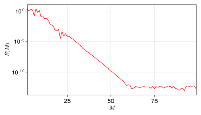
Figure 7. Convergence of eigenvalues as $M$ increases.

8.2. $K_{ij}$’s from $K_{i}$’s

Here we will consider that one does not know $K_{ij}$ but only ${K_{j}:=K(G_{j})}$ using definition (9), i.e. the quantities known in standard perturbation theory. This is not an issue since we can easily obtain approximations of $K_{ij}$ by $K_{j}$ if $\lambda_{i}$ and $\lambda_{j}$ are close, using the following lemma that is based on perturbative arguments. We recall that in numerical practice, the intermediate steps to compute $K_{i}$’s enable to compute the $K_{ij}$’s. For $j\in\{1,\dots,n\}$, we define $\lambda_{j}:=\lambda^{k}(G_{j})$.

Lemma 8.1 (Deducing $K_{ij}$ from $K_{j}$).

If

$$\left|\lambda_{i}-\lambda_{j}\right|<\left|\!\left|\left(H^{0}+\mu\right)^{-\frac{\kappa}{2}}K_{j}\left(H^{0}+\mu\right)^{\frac{\kappa}{2}}\right|\!\right|^{-1},$$

then

$$K_{ij}=K_{j}\left(1+\left(\lambda_{i}-\lambda_{j}\right)K_{j}\right)^{-1}=K_{j}\sum_{m=0}^{+\infty}\left(\lambda_{j}-\lambda_{i}\right)^{m}K_{j}^{m}$$ (29)

Proof of Lemma 8.1.

We first show that

$$K_{j}-K_{ij}=\left(\lambda_{i}-\lambda_{j}\right)K_{j}K_{ij}.$$ (30)

We define $P^{\perp}_{j}:=1-P_{j}$, we have

$$K_{j}=P_{j}^{\perp}\left(\lambda_{j}-H(G_{j})\right)^{-1}P_{j}^{\perp},\qquad\qquad K_{ij}=P_{j}^{\perp}\left(\lambda_{i}-H(G_{j})\right)^{-1}P_{j}^{\perp},$$

where we used an abuse of notation because $\left(\lambda_{j}-H(G_{j})\right)^{-1}$ should be defined as a pseudo-inverse, but the pseudo-inverse is equal to this quantity on $P^{\perp}_{j}\mathcal{H}$. We have

$$K_{j}-K_{ij} =P^{\perp}_{j}\left(\left(\lambda_{j}-H(G_{j})\right)^{-1}-\left(\lambda_{i}-H(G_{j})\right)^{-1}\right)P^{\perp}_{j}$$

$$=\left(\lambda_{i}-\lambda_{j}\right)P^{\perp}_{j}\left(\lambda_{j}-H(G_{j})\right)^{-1}\left(\lambda_{i}-H(G_{j})\right)^{-1}P^{\perp}_{j}$$

$$=\left(\lambda_{i}-\lambda_{j}\right)P^{\perp}_{j}\left(\lambda_{j}-H(G_{j})\right)^{-1}P^{\perp}_{j}P^{\perp}_{j}\left(\lambda_{i}-H(G_{j})\right)^{-1}P^{\perp}_{j}$$

$$=\left(\lambda_{i}-\lambda_{j}\right)K_{j}K_{ij},$$

where we used that $P^{\perp}_{j}\left(\lambda_{j}-H(G_{j})\right)^{-1}P_{j}=P_{j}\left(\lambda_{j}-H(G_{j})\right)^{-1}P^{\perp}_{j}=0$. From (30), we write $K_{ij}\left(1+\left(\lambda_{i}-\lambda_{j}\right)K_{j}\right)=K_{j}$ so $K_{ij}=K_{j}\left(1+\left(\lambda_{i}-\lambda_{j}\right)K_{j}\right)^{-1}$. With a manipulation similar as in (26), we have

$$\left|\!\left|K_{ij}\right|\!\right|_{e}\leqslant\frac{\left|\!\left|K_{j}\right|\!\right|_{e}}{1-\left|\lambda_{i}-\lambda_{j}\right|\left|\!\left|\left(H^{0}+\mu\right)^{-\frac{\kappa}{2}}K_{j}\left(H^{0}+\mu\right)^{\frac{\kappa}{2}}\right|\!\right|},$$

and we can deduce (29). ∎

References

- [1] G. Gaeta, Perturbation Theory: Mathematics, Methods and Applications, Springer Nature, 2023.
- [2] T. Kato, Perturbation theory for linear operators, Springer, second ed., 1995.
- [3] J. A. Murdock, Perturbations: theory and methods, SIAM, 1999.
- [4] É. Polack, G. Dusson, B. Stamm, and F. Lipparini, Grassmann extrapolation of density matrices for Born–Oppenheimer molecular dynamics, J. Chem. Theory Comput., 17 (2021), pp. 6965–6973.
- [5] É. Polack, A. Mikhalev, G. Dusson, B. Stamm, and F. Lipparini, An approximation strategy to compute accurate initial density matrices for repeated self-consistent field calculations at different geometries, Mol. Phys., 118 (2020), p. e1779834.
- [6] M. Reed and B. Simon, Methods of Modern Mathematical Physics. II. Fourier analysis, self-adjointness, Academic Press, New York, 1975.
- [7] , Methods of Modern Mathematical Physics. IV. Analysis of operators, Academic Press, New York, 1978.