Modulational Instability in the Ostrovsky Equation and Related Models

Abstract.

We study the modulational instability of small-amplitude periodic traveling wave solutions in a generalized Ostrovsky equation. Specifically, we investigate the invertibility of the associated linearized operator in the vicinity of the origin and derive a modulational instability index that depends on the dispersion and nonlinearity. We then show that the small-amplitude periodic traveling waves of the Ostrovsky equation exhibit modulational instability if the wavenumber is greater than a critical value which agrees with previously found numerical results in [WJ14] both qualitatively and quantitatively. We also study the effects of surface tension on modulational instability using the index.

1. Introduction

In 1978, Ostrovsky[Ost78] proposed the Ostrovsky equation

(1.1) $$(u_{t}+\beta u_{xxx}+(u^{2})_{x})_{x}=\gamma u,$$

as a model for the unidirectional propagation of weakly nonlinear surface and internal waves of small amplitude in a rotating fluid in the long-wavelength regime. Here, $\beta$ is the dispersion coefficient, which determines the type of dispersion, and $\gamma$ is the coriolis parameter which measures the rotational effect of the earth[GS91]. The Ostrovsky equation also occurs as a model for the propagation of short pulses in nonlinear media and as a model for magneto-acoustic solitary waves in a plasma[GGS95]. Wave dynamics in relaxing medium [Vak99] are described by this equation and its reduced form (the reduced Ostrovsky equation), which omits the third derivative element. The Gardner-Ostrovsky equation, which contains both quadratic and cubic nonlinearities, can be obtained by further generalising the Ostrovsky equation [HPT99]. A brief account of the history and applications of the Ostrovsky equation can be found in [Ste20].

There has also been interest in the so-called generalized Ostrovsky equation, given by

(1.2) $$\left(u_{t}+\beta u_{xxx}+f(u)_{x}\right)_{x}-\gamma u=0,~{}x\in\mathbb{R}$$

which generalizes the nonlinearity of the dispersive medium while satisfying a power-like scaling condition in the long wavelength regime: see, for exmaple, [HPT99]. As with most nonlinear dispersive equations, the existence and dynamics of periodic traveling or solitary waves are of special interest in both (1.1) and (1.2). The existence of solitary waves and their stability in the Ostrovsky equation and its generalizations have been demonstrated in [LLW12, LV04, LL07]. In [HSS17, GP17], periodic traveling waves of the Ostrovsky equation with general nonlinearity (1.2), as well as the generalized reduced Ostrovsky equation (corresponding to $\beta=0$ above), have been formed for small values of $\gamma$ and have been shown to be spectrally stable to periodic perturbations of the same period as the wave. In [GH08], it was shown through weakly nonlinear analysis that quasi-monochromatic wave trains [Ste20] of the Ostrovsky equation are modulationally unstable in a relatively “short-wave” range $k_{c}h<kh\ll 1$ and absent in the longer wave range $kh<k_{c}h$, where $k$ is the wave-number, $h$ is the basin depth and $k_{c}$ is the critical wave number. This weakly nonlinear analysis has been extended to more general models with cubic nonlinearity (the so-called Gardner–Ostrovsky equation [WJ14, WJ15] and the Shrira equation[NSS15]). Finally, the authors’ in [BKP22] have recently investigated that the periodic traveling waves of the Ostrovsky equation (1.1) suffers high-frequency instability if $k>\sqrt[4]{4\gamma/\beta}$ for positive values of $\beta$ and no instability for negative values of $\beta$.

In the absence of rotational effects, the models (1.1) reduces to the well-studied Korteweg-de Vries (KdV) equation

$$u_{t}-\beta u_{xxx}+\left(u^{2}\right)_{x}=0,$$

which is a canonical model for the unidirectional propagation of weakly nonlinear, small amplitude water waves in the long wavelength regime: see [Lan13] and references therein. It is well known-however, that while the KdV equation explains well long-wave phenomena in a channel of water – traveling solitary and periodic waves, for example – it fails to exhibit many high-frequency phenomena such as wave breaking – the evolutionary formation of bounded solutions with infinite gradients – and peaking – the existence of bounded, steady solutions with a singular point, such as a peak or cusp. This of course should not be surprising, as the phase velocity associated with the linear part of the KdV equation poorly approximates that of the water wave equations outside the long wavelength regime. Indeed, the (non-dimensional) phase speed for unidirectional water waves can be shown to expand as

$$c_{ww}(k):=\sqrt{\frac{\tanh(k)}{k}}=1-\frac{1}{6}k^{2}+\mathcal{O}(k^{4}),~{}~{}|k|\ll 1$$

where here $k$ is the frequency of the wave. Thus, in the long wavelength regime $|k|\ll 1$ the water wave phase speed $c_{ww}(k)$ agrees up to $\mathcal{O}(k^{2})$ with the phase speed associated to the KdV equation.

In an effort to find a simple mathematical equation that could explain water wave phenomena outside of the long-wavelength regime, Whitham proposed the model

(1.3) $$u_{t}+\beta\mathcal{M}_{ww}u_{x}+\left(u^{2}\right)_{x}=0$$

where here $\mathcal{M}_{ww}$ is a Fourier multiplier with symbol

$$\widehat{\mathcal{M}_{ww}f}(k)=c_{ww}(k)\hat{f}(k).$$

The model (1.3), now referred to as the Whitham equation, balances both the full phase speed for unidirectional water waves with a canonical shallow water nonlinearity and hence, Whitham conjectured, one might expect it to be capable of predicting both breaking and peaking of water waves. This has recently been seen to be the case. Indeed, (1.3) has recently been seen to exhibit both wave breaking [Hur17] and peaking [EK13, EW19]. Additionally, (1.3) was shown in [HJ15a] to bear out the famous Benjamin-Feir, or modulational, instability of small amplitude periodic traveling waves: see also the related numerical work in [SKCK14] on the stability of large amplitude periodic waves. Taken together, it seems clear that, regardless of its rigorous connection to the full water wave problem, the dispersion generalized model (1.3) admits many interesting high-frequency features known to exist in the full water wave problem.

Given the success of (1.3) in describing water wave phenomena outside of the long-wavelength regime, a number of recent works have aimed to study such models that incorporate additional physical effects such as surface tension, constant vorticity, as well as models allowing for bidirecitonal wave propagation: see, for example, [HJ15b, CJ18, EJC19, EJMR19, JW20, JTW22, Car18] and references therein. Interestingly, these works that focus on stability may often be carried out by considering a dispersion generalized Whitham equation

(1.4) $$u_{t}+\beta\mathcal{M}u_{x}+\left(u^{2}\right)_{x}=0,$$

where here the Fourier multiplier $\mathcal{M}$

(1.5) $$\widehat{\mathcal{M}f}(k)=m(k)\hat{f}(k)$$

need only have a symbol $m(k)$ that satisfies a few simple non-degeneracy, smoothness and growth assumptions. Results for specific models, or incorporating specific physical properties, can then be immediately ascertained by substituting for $\mathcal{M}$ a specific Fourier multiplier whose symbol agrees with the associated phase velocity. For example, with the choice $m(k)=1-|k|^{\alpha}(\alpha>1)$ (1.4) is the Fractional KdV (fKdV) equation, $m(k)=1-|k|$ is the Benjamin-Ono (BO) equation, $m(k)=k\coth k$ is the Intermediate Long wave (ILW) equation and $m(k)=\sqrt{\tanh k/k}$ is the Whitham equation (1.3).

Continuing in this spirit, this current work seeks to study the existence and stability of periodic traveling wave solutions in the following dispersion-generalized Ostrovsky (gOst) equation

(1.6) $$\left(u_{t}+\beta\mathcal{M}u_{x}+(u^{2})_{x}\right)_{x}-\gamma u=0,~{}\gamma>0,~{}\beta\in\mathbb{R}\setminus\{0\},$$

where here $\mathcal{M}$ is a Fourier multiplier operator as in (1.5) which satisfies the following assumptions:

Hypothesis 1.1.

The multiplier $m(k)$ in (1.5) is assumed to satisfy the following:

1. $m$ is real valued, even and without loss of generality, $m(0)=1$,

2. there exists constants $C_{1},C_{2}>0$ and $\alpha\geqslant-1$ such that

   $$C_{1}k^{\alpha}\leqslant m(k)\leqslant C_{2}k^{\alpha}$$

   for $k\gg 1$,

3. for each fixed $n=2,3,\ldots$ we have $m(k)\neq m(nk)$ for all $k>0$.

The model (1.6) can thus be thought of as an extension of (1.4) that incorporates rotational effects. Notice (1.6) recovers the standard Ostrovsky equation (1.1) by choosing $\mathcal{M}=-\partial_{x}^{2}$. Further, one can take $m(k)=1+|k|^{\alpha}$, $m(k)=1+|k|$, $m(k)=k\coth(k)$ and $m(k)=\sqrt{\tanh(k)/k}$ to produce variants of the fKdV, BO, ILW, and Whitham equations that incorporates rotating background fluids. Note that in our work, hypotheses (H1) and (H2) above are essential for the proof of the existence of periodic traveling waves. Hypotheses (H3) rules out the resonance between the fundamental mode and a higher harmonic. Further, note that since $m(k)$ is even, if $u(x,t)$ satisfies (1.1) for a particular choice of $\beta$ and $\gamma$, then $-u(x,-t)$ satisfies (1.1) with $\beta$ and $\gamma$ replaced by $-\beta$ and $-\gamma$ respectively. Due to this symmetry, we restrict ourselves to the case of $\gamma>0$.

In this article, we investigate the modulational instability of small-amplitude periodic traveling waves of the gOst equation (1.6). Perturbing the stokes waves, that is, small- amplitude, one-dimensional periodic traveling waves of permanent form and constant velocity, by functions bounded in space and exponential in time usually yields a spectral problem whose spectral elements characterize the time growth rates of the perturbation. This collection of spectral elements is referred as the stability spectrum of theses waves. But the scenario is not same here. In order to study the modulational instability, we need to study the spectrum for small values of floquet exponent. The differential operator becomes singular for very small values of floquet exponent and hence the results found by replacing the study of invertibility by the study of the spectrum will not be uniform for small values of floquet exponent, that is, the set of values of amplitude for which these results are valid depends upon floquet exponent, which should not be the case. Hence, we can not study modulational instability by converting the invertibility problem into the spectral problem and we instead study the invertibility problem directly.

To state our main result, note that the dispersion relation associated to (1.6) is given by

(1.7) $$\omega(k)=\beta km(k)+\dfrac{\gamma}{k}$$

while the corresponding phase and group velocities are given by

(1.8) $$c_{p}(k):=\frac{\omega(k)}{k}=\beta m(k)+\dfrac{\gamma}{k^{2}}\quad\text{and}\quad c_{g}(k):=\dfrac{d\omega}{dk}=\beta(m(k)+km^{\prime}(k))-\dfrac{\gamma}{k^{2}},$$

respectively. We now state our main result, providing a criterion governing the modulational instability of periodic traveling waves of the generalized Ostrovsky equation (1.6) which is as follows.

Theorem 1.2 (Modulational instability index).

A $2\pi/k$-periodic traveling wave of (1.6) with sufficiently small amplitude is modulationally unstable if

(1.9) $$\Delta(k):=(c_{p}(k)-c_{p}(2k))\frac{dc_{g}(k)}{dk}<0$$

where $c_{p}$ and $c_{g}$ are phase and group velocities respectively given in (1.8). It is modulationally stable if $\Delta(k)>0$.

From Theorem 1.2, $\Delta(k)$ can change sign using two mechanishms - first when $c_{p}(k)=c_{p}(2k)$, that is, phase velocities of first and second harmonic coincide, and second when $\frac{dc_{g}(k)}{dk}=0$, that is, group velocity has a critical value. As an immediate corollary of Theorem 1.2, we obtain modulational instability in the Ostrovsky equation (1.1).

Corollary 1.3 (Modulational instability).

For a fixed $\gamma>0$, a $2\pi/k$-periodic traveling wave of the Ostrovsky equation (1.1) with sufficiently small amplitude is modulationally unstable if $k>k_{c}$ where

$$\begin{cases}k_{c}=\left(\dfrac{\gamma}{3|\beta|}\right)^{1/4}&\quad\text{ if }\beta>0,\\ k_{c}=\left(\dfrac{\gamma}{4|\beta|}\right)^{1/4}&\quad\text{ if }\beta<0\end{cases}$$

and it is modulationally stable otherwise.

For $\beta=1$ and $\gamma=1$, the value of $k_{c}$ in Theorem 1.2 is approximately $0.760$ which agrees with critical wavenumber obtained by Whitfield and Johnson in [WJ14]. In addition, they mention that the instability is caused as group velocity has a critical value at $k_{c}$ which in accordance with our analysis for $\beta>0$. We show that for $\beta<0$, modulational instability is caused by coinciding phase velocities of first and second harmonic at $k_{c}$.

Remark 1.4.

From Corollary (1.3) we see that, regardless of the sign of $\beta$, the critical frequency $k_{c}$ satisfies

$$k_{c}\sim\gamma^{1/4},~{}~{}{\rm for}~{}~{}0<\gamma\ll 1.$$

Thus, one may think this suggests that all periodic traveling wave solutions of the KdV equation (corresponding essentially to $\gamma=0$) exhibit a modulational instability. This is, in fact not the case, as it is actually known that all periodic traveling waves in the KdV equation are modulationally stable (in fact, spectrally stable to general localized and bounded perturbations) [BJ10, BJK11, BD09]. This emphasizes the singular nature of the $\gamma\to 0^{+}$ limit, and results about the associated $\gamma=0$ model can not be directly inferred from taking $\gamma\to 0^{+}$ in our analysis.

This article is organized as follows. In Section 2, the existence of a family of periodic traveling waves is shown using a standard argument based on implicit function theorem and Lyapunov-Schmidt reduction. Moreover, we obtain a small-amplitude expansion of these periodic traveling waves. We linearize (1.6) about the obtained periodic traveling wave and examine the invertibility of the linearized operator resulting in a modulational instability index in Section 3. Using modulational instability index calculated in Section 3, we study modulational instability for different equations in Section 4. We also incorporate capillary effects and check how the surface tension affect the modulational instability.

Notations

The following notations are going to be used throughout the article. Let us assume $L^{2}(\mathbb{R})$ denotes the set of real or complex-valued, lebesgue measurable functions $f(x)$ over $\mathbb{R}$ such that

$$\|f\|_{L^{2}(\mathbb{R})}=\Big{(}\frac{1}{2\pi}\int_{\mathbb{R}}|f|^{2}~{}dx\Big{)}^{1/2}<+\infty\quad$$

and $L^{2}(\mathbb{T})$ denotes the space of $2\pi$-periodic, measurable, real or complex-valued functions over $\mathbb{R}$ such that

$$\|f\|_{L^{2}(\mathbb{T})}=\Big{(}\frac{1}{2\pi}\int^{2\pi}_{0}|f|^{2}~{}dx\Big{)}^{1/2}<+\infty.$$

For $f\in L^{1}(\mathbb{R})$, the Fourier transform of $f$ is written as $\hat{f}$ and defined by

$$\hat{f}(t)=\frac{1}{\sqrt{2\pi}}\int_{\mathbb{R}}f(x)e^{-itx}dx$$

It follows from Parseval Theorem that if $f\in L^{2}(\mathbb{R})$ then $\|\hat{f}\|_{L^{2}(\mathbb{R})}=\|{f}\|_{L^{2}(\mathbb{R})}$. Moreover, for any $s\in\mathbb{R}$, let $H^{s}(\mathbb{R})$ consist of tempered distributions such that

$$\|f\|_{H^{s}(\mathbb{R})}=\left(\int_{\mathbb{R}}(1+|t|^{2})^{s}|\hat{f}(t)|^{2}dt\right)^{\frac{1}{2}}<+\infty$$

Furthermore, the $L^{2}(\mathbb{T})$-inner product is defined as

(1.10) $$\langle f,g\rangle=\frac{1}{2\pi}\int^{2\pi}_{0}f(z)\overline{g}(z)~{}dz=\sum_{n\in\mathbb{Z}}\widehat{f}_{n}\overline{\widehat{g}_{n}}.$$

For any $k\in\mathbb{N}$, let $H^{k}(\mathbb{T})$ be the space of $L^{2}(\mathbb{T})$ functions whose derivatives up to $k$th order are all in $L^{2}(\mathbb{T})$. Let $H^{\infty}(\mathbb{T})=\bigcap_{k=1}^{\infty}H^{k}(\mathbb{T})$. Moreover, the commutator of two operators acting on a Hilbert space is defined by the following

$$[F,G]:=F\circ G-G\circ F.$$

2. Asymptotically small-amplitude periodic traveling waves

To begin, we seek periodic traveling wave solutions of (1.6). Here and throughout our work, we will always assume the symbol $m(k)$ associated with the Fourier multiplier $\mathcal{M}$ satisfies (H1)-(H3) in Hypothesis 1.1. To this end we make a change of variables $z:=k(x-ct)$, where $k>0$ is the wave number and $c$ is the speed of the wave, and note that if $u$ is a $2\pi/k$-periodic traveling wave solution of $\eqref{eq:gost}$ then the function $w(z):=u(k(x-ct),t)$ is a $2\pi$-periodic solution of

(2.1) $$-ck^{2}w^{\prime\prime}+\beta k^{2}\mathcal{M}_{k}w^{\prime\prime}+k^{2}(w^{2})^{\prime\prime}-\gamma w=0.$$

Note that $m(k)$ is assumed to be real-valued and even. Consequently, (2.1) is invariant under translation ($z\mapsto z+z_{0}$) and $z\mapsto-z$ and therefore, we may assume that $w$ is even. Also, since (2.1) does not possess scaling invariance, we may not a priori assume that $k=1$. In fact, the modulational instability results obtained below depends on the wavenumber $k$ of the background periodic wave.

For fixed $\beta$ and $\gamma$, define the operator $F:H_{\rm even}^{\alpha+2}(\mathbb{T})\times\mathbb{R}\times\mathbb{R}^{+}\to L^{2}(\mathbb{T})$ as

$$F(w,c;k)=-ck^{2}w^{\prime\prime}+\beta k^{2}\mathcal{M}_{k}w^{\prime\prime}+k^{2}(w^{2})^{\prime\prime}-\gamma w.$$

Note that $F$ is well defined by a elementary Sobolev embedding argument. We seek a non-trivial $2\pi$-periodic solution $w$ of (2.1) in $H_{\rm even}^{\alpha+2}(\mathbb{T})$ with $c\in\mathbb{R}$ and $k>0$ such that

$$F(w,c;k)=0.$$

To this end, note that $F(0,c;k)=0$ for all $c\in\mathbb{R}$ and $k>0$ and,

$$\ker\left(\partial_{w}F(0,c;k)\right)=\ker\left(ck^{2}\partial_{z}^{2}+\beta k^{2}\mathcal{M}_{k}\partial_{x}^{2}-\gamma\right)={\rm span}\left\{\cos(z)\right\}$$

provided that

$$c=c_{0}=\frac{\gamma}{k^{2}}+\beta m(k);$$

the kernel is trivial otherwise. Using a Lyapunov-Schmidt argument, one can thus establish the existence of a one-parameter family of non-trivial, even solutions of $F(w,c;k)$ bifurcating from $w\equiv 0$ and $c=c_{0}$. This argument is elementary and follows the same lines as those in [EK09], and is hence omitted here. The result of this analysis is summarized in the following.

Theorem 2.1.

Consider the following wavenumbers depending on the sign of $\beta$,

1. for $\beta<0$, all $k>0$, and

2. for $\beta>0$, all $k>0$ but those satisfying $k^{2}\left(m(kn)-m(k)\right)=\dfrac{\gamma(n^{2}-1)}{\beta n^{2}}$ ; $2\leq n\in\mathbb{N}$.

Then, for all such wavenumbers $k$, a one parameter family of solutions of (2.1) exists, given by $u(x,t)=w(a;k)(k(x-c(a;k)t))$ for $a\in\mathbb{R}$ and $|a|$ sufficiently small; $w(a;k)(\cdot)$ is $2\pi$-periodic, even and smooth in its argument, and $c(a;k)$ is even in $a$; $w(a;k)$ and $c(a;k)$ depend analytically on $a$ and $k$. Moreover,

(2.2) $$w(a;k)(z)=a\cos(z)+a^{2}A_{2}\cos 2z+a^{3}A_{3}\cos 3z+O(a^{4}),$$

and

(2.3) $$c(a;k)=c_{0}+a^{2}c_{2}+O(a^{6})$$

as $a\to 0$, where

$$c_{0}=\frac{\gamma}{k^{2}}+\beta m(k)$$

and

$$c_{2}=A_{2},\quad A_{2}=\dfrac{2k^{2}}{3\gamma+4\beta k^{2}(m(k)-m(2k))}\quad and\quad A_{3}=\dfrac{9k^{2}A_{2}}{8\gamma+9\beta k^{2}(m(k)-m(3k))}.$$

3. Modulational Instability Index

Throughout this section, let $w=w(x;a,k)$ with $k>0$ and $|a|\ll 1$ be a small amplitude $2\pi/k$-periodic traveling wave solution of (1.6) with wave speed $c=c(a;k)$, whose existence follows from Theorem 2.1 above. The goal of this section is to study the modulational stability of the wave $w$.

Linearizing (1.6) about $w$ in the spatial frame of reference $z=k(x-ct)$ we arrive at the linear evolution equation

$$k(v_{t}-ckv_{z}+\beta k\mathcal{M}_{k}v_{z}+2k(wv)_{z})_{z}=\gamma v.$$

governing the perturbation $v(z,t)$. We seek a solution of the form $v(z,t)=e^{\frac{\lambda}{k}t}\tilde{v}(z)$, $\lambda\in\mathbb{C}$ and $\tilde{v}\in L^{2}(\mathbb{R})$ to arrive at

(3.1) $$\mathcal{T}^{\lambda}_{k,a}\tilde{v}:=(\lambda\partial_{z}+k^{2}\partial^{2}_{z}(-c+\beta\mathcal{M}_{k}+2w)-\gamma)\tilde{v}=0,$$

where here $\mathcal{T}^{\lambda}_{k,a}:L^{2}(\mathbb{R})\to L^{2}(\mathbb{R})$ is considered as a closed, densely defined linear operator.

Definition 3.1.

The periodic traveling wave solution $w$ of (1.6) is spectrally stable with respect to square integrable perturbations if the operator $\mathcal{T}^{\lambda}_{k,a}$ is invertible on $L^{2}(\mathbb{R})$ for every $\lambda\in\mathbb{C}$ with $\Re(\lambda)>0$. Otherwise, it is deemed to be spectrally unstable.

Remark 3.2.

Note that since (3.1) is invariant under the transformation $(v,\lambda)\mapsto(\bar{v},\bar{\lambda})$, as well as the transformation $(z,\lambda)\mapsto(-z,-\lambda)$, the set of $\lambda\in\mathbb{C}$ where the operator $\mathcal{T}^{\lambda}_{k,a}$ fails to be invertible is symmetric with respect to reflections about the real and imaginary axes. Consequently, $w$ is spectrally stable if and only if $\mathcal{T}^{\lambda}_{k,a}$ is invertible for all $\lambda\in\mathbb{C}$ with $\Re(\lambda)\neq 0$.

Since the coefficients of the operator $\mathcal{T}^{\lambda}_{k,a}$ are $2\pi$-periodic, we can use the Floquet theory such that all solutions of (3.1) in $L^{2}(\mathbb{R})$ or $C_{b}(\mathbb{R})$ are of the form $\tilde{v}(z)=e^{i\xi z}V(z)$ where $\xi\in\left(-1/2,1/2\right]$ is the Floquet exponent and $V$ is a $2\pi$-periodic function, see [Har08] for a comparable circumstance.

Lemma 3.3.

The linear operator $\mathcal{T}^{\lambda}_{k,a}$ is invertible in $L^{2}(\mathbb{R})$ if and only if the linear operators

(3.2) $$\mathcal{T}^{\lambda}_{k,a,\xi}:=\lambda(\partial_{z}+i\xi)+k^{2}(\partial_{z}+i\xi)^{2}(-c+\beta e^{i\xi z}\mathcal{M}_{k}e^{-i\xi z}+2w)-\gamma$$

acting in $L^{2}(\mathbb{T})$ with domain $H^{\alpha+2}(\mathbb{T})$ are invertible for all $\xi\in\left(-\frac{1}{2},\frac{1}{2}\right]$. Moreover, $\mathcal{T}^{\lambda}_{k,a,\xi}$ is invertible in $L^{2}(\mathbb{T})$ if and only if zero is not an $L^{2}(\mathbb{T})$-eigenvalue of $\mathcal{T}^{\lambda}_{k,a,\xi}$.

Proof.

We refer readers to [Har11, Joh13] for detailed proofs in similar situations. It is straightforward to adapt those results to our case. ∎

Lemma 3.3 reduces the invertibility problem (3.1) in $L^{2}(\mathbb{R})$ to a one-parameter family of invertibility problems

(3.3) $$\mathcal{T}^{\lambda}_{k,a,\xi}\phi:=(\lambda(\partial_{z}+i\xi)+k^{2}(\partial_{z}+i\xi)^{2}(-c+\beta e^{i\xi z}\mathcal{M}_{k}e^{-i\xi z}+2w)-\gamma)\phi=0$$

in $L^{2}(\mathbb{T})$ indexed by $\xi\in\left(-\frac{1}{2},\frac{1}{2}\right)$. From Definition 3.1, it follows that the periodic traveling wave $w$ is spectrally unstable with respect to square integrable perturbations in $L^{2}(\mathbb{R})$ if and only if for some $\xi\in\left(-\frac{1}{2},\frac{1}{2}\right]$ the operator $\mathcal{T}^{\lambda}_{k,a,\xi}$ acting on $L^{2}(\mathbb{T})$ has non-trivial kernel for some $\lambda\in\mathbb{C}$ with $\Re(\lambda)>0$.

We now list some properties of the operator $\mathcal{T}^{\lambda}_{k,a,\xi}$, which may be readily verified by direct calculation.

Proposition 3.4 (Symmetric Property).

The operator $\mathcal{T}^{\lambda}_{k,a,\xi}$ acting on $L^{2}(\mathbb{T})$ has following properties.

1. $\mathcal{T}^{\lambda}_{k,a,\xi}(z)=\overline{\mathcal{T}^{-\overline{\lambda}}_{k,a,\xi}(-z)}$

2. $\mathcal{T}^{\lambda}_{k,a,\xi}=\overline{\mathcal{T}^{\overline{\lambda}}_{k,a,-\xi}}$

We now set forth the study of the $L^{2}(\mathbb{T})$-kernel of the operator $\mathcal{T}^{\lambda}_{k,a,\xi}$ for $\xi\in\left(\frac{1}{2},\frac{1}{2}\right]$ and $|a|$ sufficiently small. Note that, thanks to Proposition 3.4(2), it is sufficient to take $\xi\in[0,1/2]$. Since $k$ is fixed, in what follows, we denote $\mathcal{T}^{\lambda}_{k,a,\xi}$ by $\mathcal{T}^{\lambda}_{a,\xi}$.

We begin by discussing the case $a=0$, corresponding to the trivial solution $w=0$. A straightforward Fourier calculation yields that

(3.4) $$\mathcal{T}^{\lambda}_{0,\xi}e^{inz}=\left(i\lambda(n+\xi)+\gamma((n+\xi)^{2}-1)+\beta k^{2}(n+\xi)^{2}(m(k)-m(k(n+\xi)))\right)e^{inz}=0$$

for all $n\in\mathbb{Z}$ and $\xi\in\left[0,1/2\right]$. The kernel of $\mathcal{T}^{\lambda}_{0,\xi}$ is thus non-trivial when

(3.5) $$\lambda=i\left(\gamma\left(n+\xi-\dfrac{1}{n+\xi}\right)+n\beta k^{2}(m(k)-m(k(n+\xi)))\right)=:i\Omega_{n,\xi},\quad n\in\mathbb{Z}.$$

and hence the trivial solution $w=0$ of (1.6) is spectrally stable to square integrable perturbations as expected. Moreover, for $|a|$ small, because of Proposition 3.4, values of $\lambda$ in (3.5) will bifurcate to leave imaginary axis only when two of them collide on imaginary axis. Therefore, we obtain instability for small $|a|$ if for some $\lambda$ in (3.5), the kernel of $\mathcal{T}^{\lambda}_{0,\xi}$ is at least two-dimensional. Since we are only concerned with modulational (in)stability, we will only consider small values of $|\xi|$ and $|\lambda|$.

In particular, notice that the two values $\Omega_{1,\xi}$ and $\Omega_{-1,\xi}$ collide at $\lambda=0$ when $\xi=0$: for all other $n\in\mathbb{N}$ and $\xi$ we have $\Omega_{n,\xi}\neq 0$. Furthermore, the two-dimensional generalized kernel for $\mathcal{T}^{0}_{0,0}$ can be continued into a two-dimensional critical subspace

$$\Sigma_{0,\xi}=\ker\left(\mathcal{T}^{i\Omega_{1,\xi}}_{0,\xi}\right)\oplus\ker\left(\mathcal{T}^{i\Omega_{-1,\xi}}_{0,\xi}\right)$$

with ($\xi$-independent) orthogonal basis

(3.6) $$\phi_{1}(z)=\cos(z),\quad\phi_{2}(z)=\sin(z).$$

For all other values of $n\neq-1,1$, the kernel of $\mathcal{T}^{i\Omega_{n,0}}_{0,0}$ is one-dimensional and therefore, from Proposition 3.4(1), can not lead to instability for $|(a,\xi)|\ll 1$. We thus aim to track how the values $\Omega_{\pm 1,0}$ bifurcate from the origin for $|(a,\xi)|\ll 1$. To this end, we note that, for $|a|$ and $\xi$ small, the operator$\mathcal{T}^{\lambda}_{a,\xi}$ is a perturbation of $\mathcal{T}^{\lambda}_{0,0}$ with

$$\|\mathcal{T}^{\lambda}_{a,\xi}-\mathcal{T}^{\lambda}_{0,0}\|_{L^{2}(\mathbb{T})\to L^{2}(\mathbb{T})}=O(|a|+|\xi|)$$

uniformly in operator norm as $|a|,\xi\to 0$. Consequently, for $|(a,\xi)|\ll 1$ there can be only two values $\lambda=i\Omega_{\pm 1,a,\xi}$ in a sufficiently small neighborhood of the origin where the operator $\mathcal{T}^{\lambda}_{a,\xi}$ fails to be invertible and, further, the functions

$$(a,\xi)\mapsto\Omega_{\pm 1,a,\xi}$$

are analytic in $(a,\xi)$ for $|(a,\xi)|\ll 1$ and limit back to $\Omega_{\pm 1,0}=0$ as $(a,\xi)\to(0,0)$. Further, one has a two-dimensional critical subspace

$$\Sigma_{a,\xi}=\ker\left(\mathcal{T}^{i\Omega_{1,a,\xi}}_{a,\xi}\right)\oplus\ker\left(\mathcal{T}^{i\Omega_{-1,a,\xi}}_{a,\xi}\right)$$

which is an analytical continuation of that found at $a=0$ above.

Our goal is now to track the critical values $\lambda(a,\xi)=\Omega_{\pm 1,a,\xi}$ for $|(a,\xi)|\ll 1$. To this end, our strategy is essentially to project the operator equation $\mathcal{T}^{\lambda}_{a,\xi}v=0$ onto the two-dimensional critical subspace $\Sigma_{a,\xi}$ above. More precisely, we will compute a suitable basis $\{\phi_{j}(z;a,\xi)\}_{j=1,2}$ for $\Sigma_{a,\xi}$ and then compute the $2\times 2$ matrix

(3.7) $$B_{ij}=\frac{\langle\mathcal{T}^{\lambda}_{a,\xi}\phi_{i}(z;a,\xi),\phi_{j}(z;a,\xi)\rangle}{\langle\phi_{i}(z;a,\xi),\phi_{j}(z;a,\xi)\rangle}.$$

The critical values $\lambda(a,\xi)$ are then found by solving the algebraic equation

(3.8) $$\det(\mathcal{B}^{\lambda}_{a,\xi})=0$$

for the variable $\lambda$. It remains then to find a suitable basis for the critical subspace $\Sigma_{a,\xi}$, and then to compute the appropriate projections above.

To compute a basis for $\Sigma_{a,\xi}$ that is compatible with $\Sigma_{0,\xi}$, note that differentiating the profile equation (2.1) with respect to $z$ and $a$ gives

$$\mathcal{T}^{0}_{a,0}(\partial_{z}w)=0,\quad\mathcal{T}^{0}_{a,0}(\partial_{a}w)=0.$$

Using the expansions in Theorem 2.1, we thus obtain a normalized basis for the critical subspace $\Sigma_{a,0}$, i.e. the generalized kernel of $\mathcal{T}^{0}_{a,0}$, as

(3.9) $$\phi_{1}(z;a,0)=-\frac{1}{a}(\partial_{z}w)(z)=\sin z+2aA_{2}\sin 2z+3a^{2}A_{3}\sin 3z+O(a^{4})$$

and

(3.10) $$\phi_{2}(z;a,0)=(\partial_{a}w)(z)=\cos z+2aA_{2}\cos 2z+3a^{2}A_{3}\cos 3z+O(a^{4}),$$

where here the values $A_{j}$ are as in Theorem 2.1. These functions provide asymptotic extensions for the generalized kernel of $\mathcal{T}^{0}_{0,0}$ and, in fact, they provide an asymptotic extension for the ($\xi$-independent) basis of the critical subspace $\Sigma_{0,\xi}$ provided in (3.6). By spectral perturbation theory, it follows that the functions $\phi_{1}(\cdot;a,0)$ and $\phi_{2}(\cdot;a,0)$ continue into a $\xi$-dependent basis for the critical subspace $\Sigma_{a,\xi}$ for $|(a,\xi)|\ll 1$. We note, however, that as in [Joh13, HJ15a, HJ15b], the variations in the basis functions $\phi_{j}(\cdot;a,\xi)$ does not play a role in the asymptotic calculation below as they contribute only to higher-order terms than what are needed here. Thus, below, the calculations are done with the $\xi$-independent basis $\phi_{j}(\cdot;a,0)$.

Continuing our strategy, we now compute the action of $\mathcal{T}^{\lambda}_{a,\xi}$ on the critical subspace $\Sigma_{a,\xi}$.Here $\langle\hskip 2.00749pt\cdot\hskip 2.00749pt,\hskip 2.00749pt\cdot\hskip 2.00749pt\rangle$ denotes the $L^{2}(\mathbb{T})$- inner product as defined in (1.10). Now, for $\xi$ and $|a|$ sufficiently small, we expand $\mathcal{T}^{\lambda}_{a,\xi}$ using Baker-Campbell-Hausdorff formula as

(3.11) $$\mathcal{T}^{\lambda}_{a,\xi}=T_{0,a}+i\xi T_{1,a}-\dfrac{\xi^{2}}{2}T_{2,a}+O(\xi^{3})$$

as $\xi\to 0$ where

$$T_{0,a}:=\mathcal{T}^{\lambda}_{a,0}=T_{0}+2k^{2}\partial z^{2}(a\cos z+a^{2}A_{2}\cos 2z)$$

$$T_{1,a}:=[\mathcal{T}^{\lambda}_{a,0},z]=T_{1}+4k^{2}\partial z(a\cos z+a^{2}A_{2}\cos 2z)$$

$$T_{2,a}:=[[\mathcal{T}^{\lambda}_{a,0},z],z]=T_{2}+4k^{2}(a\cos z+a^{2}A_{2}\cos 2z)$$

and

$$T_{0}=\mathcal{T}^{\lambda}_{0,0},\quad T_{1}=[T_{0},z]\quad\text{and}\quad T_{2}=[[T_{0},z],z].\vspace{3px}$$

Note that $T_{1,a}$ and $T_{2,a}$ are well defined in $L^{2}(\mathbb{T})$. Now, to find the action of $T_{0}$, $T_{1}$ and $T_{2}$ on the generalized kernel, we use the expansion $\mathcal{T}^{\lambda}_{0,\xi}e^{inz}$ rather than computing tedious fourier series expansions. Moreover,

$$\mathcal{T}^{\lambda}_{0,\xi}(\cos nz)=\mathcal{T}^{\lambda}_{0,\xi}\left(\dfrac{e^{inz}+e^{-inz}}{2}\right)\quad\quad\text{and}\quad\quad\mathcal{T}^{\lambda}_{0,\xi}(\sin nz)=\mathcal{T}^{\lambda}_{0,\xi}\left(\dfrac{e^{inz}-e^{-inz}}{2i}\right).$$

Consequently,

$$T_{0}(\cos nz)= -n\lambda\sin nz+\gamma(n^{2}-1)\cos nz+\beta k^{2}n^{2}(m(k)-m(kn))\cos nz,$$

$$T_{1}(\cos nz)= \lambda\cos nz+2n\gamma\sin nz+\beta k^{2}(-n^{2}km^{\prime}(kn)+2n(m(k)$$

$$-m(kn))\sin nz,$$

$$T_{2}(\cos nz)= -2\gamma\cos nz-2\beta k^{2}(m(k)-m(kn)-2nkm^{\prime}(kn)$$

$$-\dfrac{n^{2}k^{2}}{2}m^{\prime\prime}(kn))\cos nz,$$

and

$$T_{0}(\sin nz)= n\lambda\cos nz+\gamma(n^{2}-1)\sin nz+\beta k^{2}n^{2}(m(k)-m(kn))\sin nz,$$

$$T_{1}(\sin nz)= \lambda\sin nz-2n\gamma\cos nz-\beta k^{2}(-n^{2}km^{\prime}(kn)+2n(m(k)$$

$$-m(kn))\cos nz,$$

$$T_{2}(\sin nz)= -2\gamma\sin nz-2\beta k^{2}(m(k)-m(kn)-2nkm^{\prime}(kn)$$

$$-\dfrac{n^{2}k^{2}}{2}m^{\prime\prime}(kn))\sin nz.$$

Using these, we get

$$\left<\mathcal{T}^{\lambda}_{a,\xi}\phi_{1},\phi_{1}\right>= \dfrac{1}{2}(-a^{2}k^{2}A_{2}+i\xi\lambda(1+4a^{2}A_{2}^{2})-\dfrac{\xi^{2}}{2}(-2\gamma(1+a^{2}A_{2}^{2})+2a^{2}k^{2}A_{2}+\beta k^{4}(m^{\prime\prime}(k)$$

$$+16a^{2}A_{2}^{2}m^{\prime\prime}(2k))+4\beta k^{3}(m^{\prime}(k)+8a^{2}A_{2}^{2}m^{\prime}(2k)))),$$

$$\left<\mathcal{T}^{\lambda}_{a,\xi}\phi_{1},\phi_{2}\right>= \dfrac{1}{2}(\lambda(1+8a^{2}A_{2}^{2})+i\xi(-2\gamma(1+2a^{2}A_{2}^{2})+2a^{2}k^{2}A_{2}^{2}+\beta k^{3}(m^{\prime}(k)+16a^{2}A_{2}^{2}m^{\prime}(2k))),$$

$$\left<\mathcal{T}^{\lambda}_{a,\xi}\phi_{2},\phi_{1}\right>= \dfrac{1}{2}(-\lambda(1+8a^{2}A_{2}^{2})+i\xi(2\gamma(1+2a^{2}A_{2}^{2})-6a^{2}k^{2}A_{2}^{2}-\beta k^{3}(m^{\prime}(k)+16a^{2}A_{2}^{2}m^{\prime}(2k))),$$

$$\left<\mathcal{T}^{\lambda}_{a,\xi}\phi_{2},\phi_{2}\right>= \dfrac{1}{2}(-3a^{2}k^{2}A_{2}+i\xi\lambda(1+4a^{2}A_{2}^{2})-\dfrac{\xi^{2}}{2}(-2\gamma(1+a^{2}A_{2}^{2})+6a^{2}k^{2}A_{2}+\beta k^{4}(m^{\prime\prime}(k)$$

$$+16a^{2}A_{2}^{2}m^{\prime\prime}(2k))+4\beta k^{3}(m^{\prime}(k)+8a^{2}A_{2}^{2}m^{\prime}(2k)))).$$

Using above obtained expressions, for sufficiently small $\xi$ and $|a|$, we have

$$\mathcal{B}^{\lambda}_{a,\xi}= \dfrac{\lambda}{2}\begin{pmatrix}0&1\\ -1&0\end{pmatrix}+\dfrac{a^{2}}{2}\begin{pmatrix}-k^{2}A_{2}&8\lambda A_{2}^{2}\\ -8\lambda A_{2}^{2}&-3k^{2}A_{2}\end{pmatrix}+\dfrac{i\xi}{2}\begin{pmatrix}\lambda&-2\gamma+\beta k^{3}m^{\prime}(k)\\ 2\gamma-\beta k^{3}m^{\prime}(k)&\lambda\end{pmatrix}+$$

$$\dfrac{i\xi a^{2}}{2}\begin{pmatrix}4\lambda A_{2}^{2}&-2A_{2}^{2}+2k^{2}A_{2}^{2}+16\beta k^{3}A_{2}^{2}m^{\prime}(2k)\\ 2A_{2}^{2}-6k^{2}A_{2}^{2}-16\beta k^{3}A_{2}^{2}m^{\prime}(2k)&4\lambda A_{2}^{2}\end{pmatrix}+$$

$$\dfrac{-\xi^{2}}{2}(-2\gamma+\beta k^{4}m^{\prime\prime}(k)+4\beta k^{3}m^{\prime}(k))\begin{pmatrix}1&0\\ 0&1\end{pmatrix}+$$

$$\dfrac{-\xi^{2}a^{2}}{2}(-2\gamma A_{2}^{2}+6k^{2}A_{2}+16\beta k^{4}A_{2}^{2}m^{\prime\prime}(2k)+32\beta k^{3}A_{2}^{2}m^{\prime}(2k))\begin{pmatrix}1&0\\ 0&1\end{pmatrix}+O(\xi^{3}+a^{3}).$$

Assume $\lambda=iX$, then $\det(\mathcal{B}^{\lambda}_{a,\xi})=0$ is a quadratic in $X$ with discriminant

(3.12) $$\xi^{4}(\beta k^{3}(km^{\prime\prime}(k)+2m^{\prime}(k))+2\gamma)^{2}+\xi^{2}a^{2}\left(\dfrac{2\gamma+\beta k^{3}(km^{\prime\prime}(k)+2m^{\prime}(k))}{3\gamma+4\beta k^{2}(m(k)-m(2k))}\right)+O(|a|\xi(\xi^{3}+a^{3}))$$

Therefore, for small $|a|$, we can choose $\xi$ sufficiently small such that $\lambda$ is away from the imaginary axis if

(3.13) $$\dfrac{2\gamma+\beta k^{3}(km^{\prime\prime}(k)+2m^{\prime}(k))}{3\gamma+4\beta k^{2}(m(k)-m(2k))}<0.$$

The sign of the expression in the left above agrees with the modulational instability index, $\Delta(k)$ in Theorem 1.2.

4. Application to Specific Models

In this section, we apply the general result from Theorem 1.2 to a number of specific models. When possible, we compare our results to previously known results.

4.1. Ostrovsky equation

As a first application, we apply Theorem 1.2 to the classical Ostrovsky equation (1.1). Note that (1.1) corresponds to our generalized-dispersion model (1.6) with the choice

(4.1) $$\mathcal{M}=1+\partial_{x}^{2},~{}~{}{\rm i.e.}~{}~{}m(k)=1-k^{2}.$$

The symbol $m(k)$ clearly satisfies Hypotheses 1.1 (H1), (H2) ($\alpha=2$, $C_{1}=1$ and $C_{2}=2$), and (H3) ($m$ is strictly decreasing for $k>0$). Consequently, we obtain asymptotically small periodic traveling wave solutions from Theorem 2.1 along with asymptotic expansions provided explicitly by substituting $m(k)=1-k^{2}$ into (2.2).

In this case, the corresponding phase and group velocities are given explicitly by

$$c_{p}(k)=\beta\left(1-k^{2}\right)+\frac{\gamma}{k^{2}}~{}~{}{\rm and}~{}~{}c_{g}(k)=\beta\left(1-3k^{2}\right)-\frac{\gamma}{k^{2}}.$$

The qualitative properties clearly depend on the sign of $\beta$. For $\beta>0$, the group velocity $c_{g}$ attains a global maxima (for $k>0$) at $k=k_{c}=\left(\dfrac{\gamma}{3|\beta|}\right)^{1/4}$ and is monotonically increasing for $k\in(0,k_{c})$ and monotonically decreasing for $k>k_{c}$. Further, in this case the phase speed $c_{p}(k)$ is strictly decreasing for $k>0$, and hence in this case one has

$$\Delta(k)>0~{}~{}{\rm for}~{}~{}k\in(0,k_{c})~{}~{}~{}{\rm and}~{}~{}~{}\Delta(k)<0~{}~{}{\rm for}~{}~{}k>k_{c}.$$

This establishes the modulational instability and stability result in Corollary 1.3 in the case $\beta>0$.

Similarly, when $\beta<0$ the group velocity is strictly increasing for all $k>0$, while $c_{p}(k)-c_{p}(2k)$ changes signs exactly once, from positive to negative, at $k_{c}=\left(\dfrac{\gamma}{4|\beta|}\right)^{1/4}$. This establishes Corollary 1.3 in the case $\beta<0$. Notice, in particular, that the mechanisms accounting for the modulational instabilities in the case $\beta>0$ are different from those in the $\beta<0$ case.

4.2. Ostrovsky-fKdV equation

The Ostrovsky-fractional KdV equation

(4.2) $$\left(u_{t}+\beta(1-|\partial_{x}|^{\delta})u_{x}+(u^{2})_{x}\right)_{x}-\gamma u=0,~{}\gamma>0,~{}\beta\in\mathbb{R}\setminus\{0\}$$

can be obtained from (1.6) by choosing $m(k)=1-|k|^{\delta}$, $\delta>1/2$. In this case, the symbol $m(k)$ clearly satisfies Hypotheses 1.1 (H1), (H2) ($\delta=\alpha$, $C_{1}=1$, and $C_{2}=2$), and (H3) ($m$ is strictly decreasing for $k>0$). As above, we can obtain asymptotically small amplitude periodic travleing wave solutions of the Ostrovsky-fKdV equation from Theorem 2.1 by substituting $m(k)=1-|k|^{\delta}$. Applying precisely the same reasoning as in the previous section for the classical Ostrovsky equation, we obtain the following result.

Corollary 4.1.

For a fixed $\gamma>0$, a $2\pi/k$-periodic traveling wave of the Ostrovsky-fKdV equation (4.2) with sufficiently small amplitude is modulationally unstable if $k>k_{c}$, where

$$\begin{cases}k_{c}=\left(\dfrac{2\gamma}{\delta(1+\delta)|\beta|}\right)^{1/(2+\delta)}&\quad\text{ if }\beta>0,\\ k_{c}=\left(\dfrac{3\gamma}{4(2^{\delta}-1)|\beta|}\right)^{1/(2+\delta)}&\quad\text{ if }\beta<0.\end{cases}$$

and it is modulationally stable otherwise.

Proof.

The proof is same as the Ostrovsky equation in Section 4.1 ∎

4.3. Ostrovsky-ILW equation

The Intermediate Long Wave (ILW) equation is given by

$$u_{t}+\beta\mathcal{M}u_{x}+\left(u^{2}\right)_{x}=0$$

where here $\mathcal{M}$ is a Fourier multiplier with symbol $m(k)=k\coth(k)$. The ILW is well-known to describe long internal gravity waves in a two-layer stratified fluid, with the lower layer having a large finite depth. By adding rotational effects, we can obtain an Ostrovsky-ILW equation by making the choice $m(k)=k\coth(k)$ in (1.6). The symbol $m(k)$ clearly satisfies Hypotheses 1.1 (H1), (H2) ($\alpha=2$, $C_{1}=1$ and $C_{2}=2$), and (H3) ($m$ is strictly increasing for $k>0$). As above, we can obtain asymptotically small amplitude periodic travleing wave solutions of the Ostrovsky-ILW equation from Theorem 2.1. Again applying the same reasoning as in Section 4.1, we obtain the following result.

Corollary 4.2.

For a fixed $\gamma>0$, a $2\pi/k$-periodic traveling wave of the Ostrovsky-ILW equation (1.1) with sufficiently small amplitude is modulationally unstable if $k>k_{c}$, where $k_{c}$ is the unique real solution of following equations

$$\begin{cases}k^{2}(2k\coth{2k}-k\coth{k})-\dfrac{3\gamma}{4|\beta|}=0&\quad\text{ if }\beta>0,\\ ~{}\\ k^{3}(-4k\operatorname{csch}^{2}{k}+2k^{2}\coth{k}\operatorname{csch}^{2}{k}+2\coth{k})-\dfrac{2\gamma}{|\beta|}=0&\quad\text{ if }\beta<0\end{cases}$$

and it is modulationally stable otherwise.

Proof.

The proof is same as the Ostrovsky equation in Section 4.1 Note that while we lack an explicit formula for the critical frequency $k_{c}$, it can of course be numerically approximated. ∎

4.4. Ostrovsky-Whitham equation

Continuing as above, we may consider an Ostrovsky variant of the well-studied Whitham equation (1.3) by choosing

(4.3) $$m(k)=\sqrt{\frac{\tanh k}{k}}$$

The symbol $m(k)$ clearly satisfies Hypotheses 1.1 (H1), (H2) ($\alpha=-1/2$,$C_{1}=1$ and $C_{2}=2$), and (H3) ($m$ is strictly decreasing for $k>0$). As above, we can obtain asymptotically small amplitude periodic travleing wave solutions of the Ostrovsky-fKdV equation from Theorem 2.1. In this case, our Theorem 1.2 gives the following result.

Corollary 4.3.

For a fixed $\gamma>0$, a $2\pi/k$-periodic traveling wave of the Ostrovsky-Whitham equation (1.1) with sufficiently small amplitude is modulationally unstable if $k>k_{c}$, where $k_{c}$ is the unique real solution of following equations

$$\begin{cases}k^{3}\left|k\dfrac{d^{2}}{dk^{2}}\left(\sqrt{\frac{\tanh k}{k}}\right)+2\dfrac{d}{dk}\left(\sqrt{\frac{\tanh k}{k}}\right)\right|-\dfrac{2\gamma}{|\beta|}=0&\quad\text{ if }\beta>0,\\ ~{}\\ k^{2}\left(\sqrt{\frac{\tanh k}{k}}-\sqrt{\frac{\tanh 2k}{2k}}\right)-\dfrac{3\gamma}{4|\beta|}=0&\quad\text{ if }\beta<0\end{cases}$$

and it is modulationally stable otherwise.

Proof.

The proof is same as the Ostrovsky equation in Section 4.1 ∎

4.5. Effects of surface tension on Modulational instability

We incorporate the capillary effects into the Ostrovsky-KdV and Ostrovsky-Whitham equations and examine how surface tension effects the modulational stability of small periodic traveling waves.

4.5.1. Ostrovsky-KdV equation with surface tension

Upon normalization, in the presence of surface tension in the Ostrovsky equation, the dispersion will change to

(4.4) $$m(k,T)=1-k^{2}+3Tk^{2}$$

where $T\geqslant 0$ is the coefficient of surface tension. For $T=0$, (4.4) reduces to (4.1).

Using Theorem 1.2, we have following results on the effects of surface tension on modulational stability in the Ostrovsky equation.

Corollary 4.4.

1. For $\beta>0$, a sufficiently small $2\pi/k$-periodic traveling wave of the Ostrovsky equation (1.1) is modulationally unstable under capillary effects if $k>k_{c}(T)$, where

   $$\begin{cases}k_{c}(T)=\left(\dfrac{\gamma}{3|\beta|(1-3T)}\right)^{1/4}&\quad\text{ if }T<1/3,\\ k_{c}(T)=\left(\dfrac{\gamma}{4|\beta|(3T-1)}\right)^{1/4}&\quad\text{ if }T>1/3,\end{cases}$$

   and it is modulationally stable otherwise.

2. For $\beta<0$, a sufficiently small $2\pi/k$-periodic traveling wave of the Ostrovsky equation (1.1) is modulationally unstable if $k>k_{c}(T)$ under capillary effects, where

   $$\begin{cases}k_{c}(T)=\left(\dfrac{\gamma}{4|\beta|(1-3T)}\right)^{1/4}&\quad\text{ if }T<1/3,\\ k_{c}(T)=\left(\dfrac{\gamma}{3|\beta|(3T-1)}\right)^{1/4}&\quad\text{ if }T>1/3,\end{cases}$$

   and it is modulationally stable otherwise.

For $T=0$, that is, when capillary effects are absent, value of $k_{c}(0)$ agrees with $k_{c}$ in Corollary 1.3. For $T>0$, we describe the modulational instability through the Figure 1. In $k$-$k\sqrt{T}$ plane, two curves are corresponding to each mechanism splitting the plane into two regions of stability and two regions of instability. Any fixed $T>0$ corresponds to a line passing through the origin of slope $\sqrt{T}$. For $T\neq 1/3$, the line through the origin only crosses one curve at a time producing one interval of stable wave numbers and one interval of unstable wave numbers. The result becomes inconclusive for $T=1/3$.

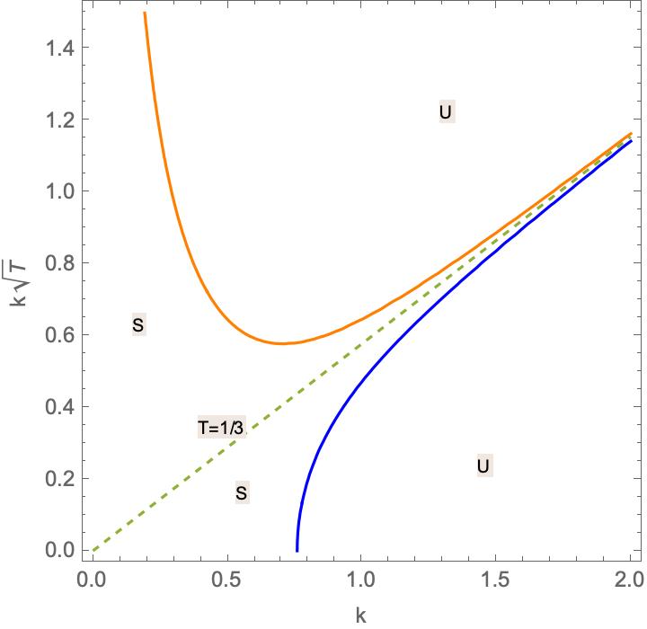
Figure 1. Stability diagram for sufficiently small, periodic wave trains of Ostrovsky equation. “S” and “U” denote stable and unstable regions. Solid curves represent roots of the stability condition (1.9), that is, $(c_{p}(k)-c_{p}(2k))\frac{dc_{g}(k)}{dk}$.

4.5.2. Ostrovsky-Whitham equation with surface tension

To incorporate the effects of surface tension into the Ostrovsky-Whitham equation we replace the

(4.5) $$m(k,T)=\sqrt{\dfrac{\tanh{k}}{k}(1+Tk^{2})},$$

where $T\geqslant 0$ is the (properly normalized) coefficient of surface tension. Note that when $T=0$, (4.5) reduces to (4.3) and hence we will only consider the case $T>0$ here.

First, note that for each fixed $T>0$ the symbol $m(\cdot,T)$ satisfies

$$m(0,T)=0\quad{\rm and}\quad\lim_{|k|\to\infty}m(k,T)=\infty.$$

Further, it is readily seen that $m(\cdot,T)$ is strictly monotone for $k>0$ provided $T>1/3$, while for $0<T<1/3$ there exists a unique $k^{*}(T)$ such that $m(\cdot,T)$ is monotone decreasing on $(0,k^{*}(T))$ and monotone increasing for $(k^{*}(T),\infty)$. In this way, the critical surface tension $T=1/3$ is often used to differentiate between the “weak” ($0<T<1/3$) and “strong” ($T>1/3$) surface tension cases.

According to Theorem 1.2, whenever factors $c_{p}(k)-c_{p}(2k)$ and $\frac{dc_{g}(k)}{dk}$ of the modulational instability index $\Delta(k)$ are zero, stability changes, where $c_{k}(p)$ and $c_{g}(k)$ are defined in (1.8). To show the explicit dependence on surface tension, we replace $c_{p}(k)$ and $c_{g}(k)$, by $c_{p}(k,T)$ and $c_{g}(k,T)$, respectively. Notice that zeros of factors $c_{p}(k,T)-c_{p}(2k,T)$ and $\frac{dc_{g}(k,T)}{dk}$ are same for fixed value of the ratio $\alpha:=\frac{\gamma}{\beta}$. Since $\gamma$ is always positive, sign of $\alpha$ agrees with that of $\beta$. We will consider the cases $\alpha>0$ and $\alpha<0$ below separately.

Case $\alpha>0$: It is straightforward to see that for each $\alpha>0$, there exists a unique $T=T_{c}(\alpha)$ such that the group velocity $c_{g}$ attains a local maxima and a local minima for $0<T<T_{c}(\alpha)$ and is monotonic for $T>T_{c}(\alpha)$. For instance, for $\alpha=0.1$, $T_{c}\approx 0.132$ and therefore, plots of $c_{g}(k,T)$ vs. $k$ for $T=0.02<T_{c}$ and $T=0.5>T_{c}$ (see Figure 2) confirm the monotonocity property of $c_{g}$. Moreover, for any $T>0$, $c_{p}(k,T)-c_{p}(2k,T)$ is changing its sign only once, see Figure 3, for instance.

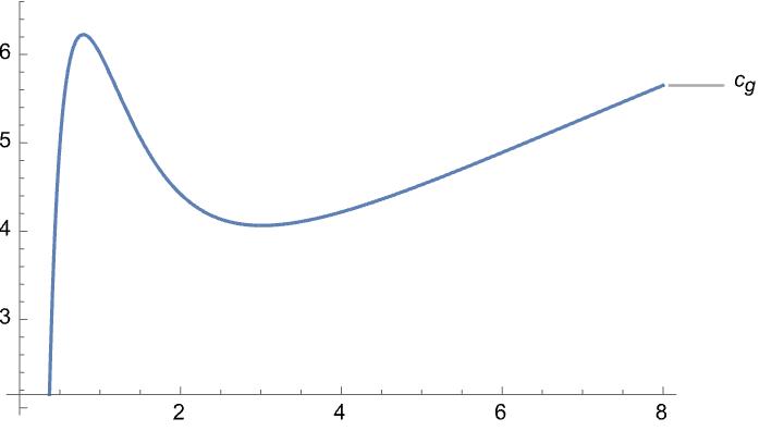
(a) $T=0.02$

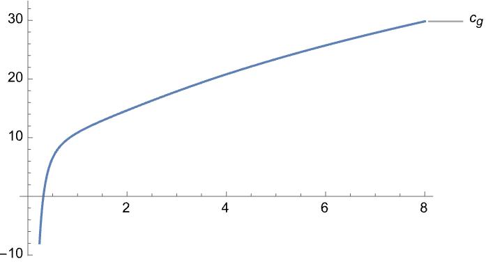
(b) $T=0.5$

Figure 2. Graph of function $c_{g}$ vs. $k$ for $\alpha=0.1$ for which $T_{c}\approx 0.132$.

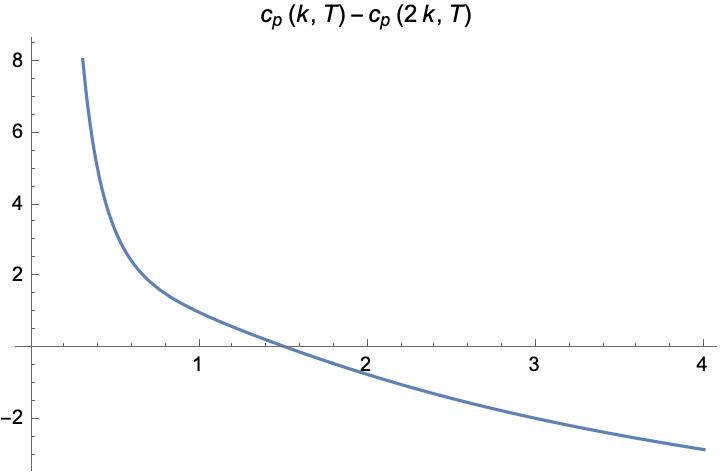
Figure 3. $c_{p}(k,T)-c_{p}(2k,T)$ vs $k$ for $T=0.2$.

Therefore, for $0<T<T_{c}(\alpha)$, there exist three critical wavenumbers $0<k_{1}<k_{2}<k_{3}$ such that sufficiently small $2\pi/k$-periodic traveling wave is modulationally stable for $k\in(0,k_{1})\cup(k_{2},k_{3})$ and modulationally unstable for $k\in(k_{1},k_{2})\cup(k_{3},\infty)$. On the other hand, for $T>T_{c}(\alpha)$ there is only one critical wave number $k_{c}>0$ such that sufficiently small $2\pi/k$-periodic traveling wave is modulationally stable for $0<k<k_{c}(T)$ and modulationally unstable for $k>k_{c}(T)$.

In [Kaw75] and [DR77], the effects of surface tension on modulational instability in the full water wave problem has been shown in $k-k\sqrt{T}$ plane. We produce a similar plot for $\alpha=0.1$ in Figure 4. In $k$-$k\sqrt{T}$ plane, two curves are corresponding to each mechanism splitting the plane into three regions of stability and three regions of instability. For $\alpha=0.1$, this can be easily seen that $T_{c}\approx 0.132$ such that for $0<T<0.132$, the line crosses both the curves producing two intervals of stable wave numbers and two intervals of unstable wave numbers. On the other hand, for $T>0.132$, the line through the origin crosses only one curve producing one interval of stable wave numbers and one interval of unstable wave numbers.

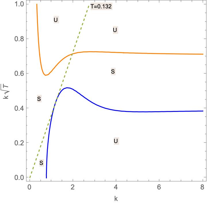
Figure 4. Stability diagram for sufficiently small, periodic wave trains of Ostrovsky-Whitham equation for $\alpha=0.1$. “S” and “U” denote stable and unstable regions. Orange curve represent roots of $c_{p}(k)-c_{p}(2k)=0$ and blue curve represent roots of $\dfrac{dc_{g}}{dk}=0$. Note in this case we have $T_{c}\approx 0.132$.

Case $\alpha<0$: For each $\alpha<0$, there exists $T=T_{c}(\alpha)$ such that for $0<T<T_{c}(\alpha)$, $c_{p}(k,T)-c_{p}(2k,T)$ changing its sign at two wavenumbers resulting in two critical wavenumbers, and for $T>T_{c}(\alpha)$, $c_{p}(k,T)-c_{p}(2k,T)$ does not change its sign (see Figure 5). On the other hand, for each $T>0$, $c_{g}$ attains extremum only once (see Figure 6) producing one critical wavenumber. Therefore, for $0<T<T_{c}(\alpha)$, there exist three critical wavenumbers such that sufficiently small $2\pi/k$-periodic traveling wave is modulationally stable for $k\in(0,k_{c_{1}})\cup(k_{c_{2}},k_{c_{3}})$ and modulationally unstable for $k\in(k_{c_{1}},k_{c_{2}})\cup(k_{c_{3}},\infty)$. For $T>T_{c}(\alpha)$, there is only one critical wave number $k_{c}$ such that sufficiently small $2\pi/k$-periodic traveling wave is modulationally stable for $0<k<k_{c}(T)$ and modulationally unstable for $k>k_{c}(T)$. The graph of $T_{c}$ vs. $\alpha$ is shown in Figure 7.

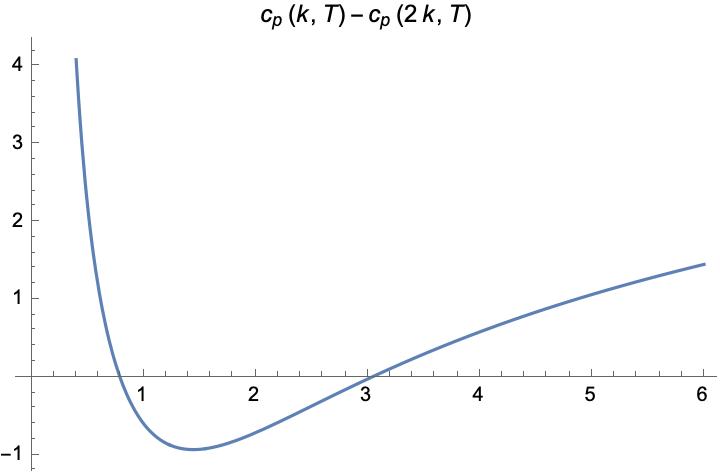
(a) $T=0.02$

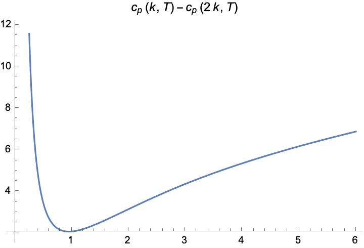
(b) $T=0.5$

Figure 5. Graph of function $c_{p}(k,T)-c_{p}(2k,T)$ vs. $k$ for $\alpha=-0.1$ for which $T_{c}=0.141$.

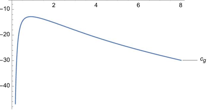
Figure 6. $c_{g}$ vs $k$ for $T=0.5$.

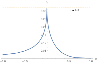
Figure 7. $T_{c}$ vs $\alpha$.

For $\alpha=-0.1$, we can see this behavior through the Figure 8. In $k$-$k\sqrt{T}$ plane, two curves are corresponding to each mechanism splitting the plane into three regions of stability and three regions of instability. For $\alpha=-0.1$, $T_{c}\approx 0.141$ such that for $0<T<0.141$, the line crosses both the curves producing two intervals of stable wave numbers and two intervals of unstable wave numbers. On the other hand, for $T>0.141$, the line through the origin crosses only one curve producing one interval of stable wave numbers and one interval of unstable wave numbers.

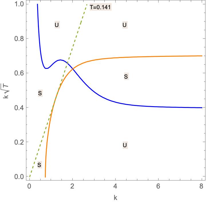
Figure 8. Stability diagram for sufficiently small, periodic wave trains of Ostrovsky-Whitham equation for $\alpha=-0.1$. “S” and “U” denote stable and unstable regions. Orange curve represent roots of $c_{p}(k,T)-c_{p}(2k,T)=0$ and blue curve represent roots of $\dfrac{dc_{g}}{dk}=0$.

Remark 4.5.

For every $\alpha<0$, there is a value of $0<T=T_{s}<T_{c}(\alpha)$ corresponding to the intersection of two curves in the Figure 8 for which there is only one interval of stable and unstable wavenumbers contrary to other values of $T$ in the interval $(0,T_{c})$.

References

- [BD09] Nate Bottman and Bernard Deconinck, KdV cnoidal waves are spectrally stable, Discrete and Continuous Dynamical Systems 25 (2009), no. 4, 1163–1180.
- [BJ10] Jared C. Bronski and Mathew A. Johnson, The modulational instability for a generalized korteweg-de vries equation, Archive for Rational Mechanics and Analysis 197 (2010), no. 2, 357–400.
- [BJK11] Jared C. Bronski, Mathew A. Johnson, and Todd Kapitula, An index theorem for the stability of periodic travelling waves of Korteweg-de Vries type, Proc. Roy. Soc. Edinburgh Sect. A 141 (2011), no. 6, 1141–1173. MR 2855892
- [BKN16] Handan Borluk, Henrik Kalisch, and David P. Nicholls, A numerical study of the Whitham equation as a model for steady surface water waves, J. Comput. Appl. Math. 296 (2016), 293–302. MR 3430140
- [BKP22] Bhavna, Atul Kumar, and Ashish Kumar Pandey, High-Frequency Instabilities of the Ostrovsky Equation, Water Waves (2022), 91–108.
- [Car18] John D. Carter, Bidirectional Whitham equations as models of waves on shallow water, Wave Motion 82 (2018), 51–61. MR 3844340
- [CJ18] Kyle M. Claassen and Mathew A. Johnson, Numerical bifurcation and spectral stability of wavetrains in bidirectional Whitham models, Stud. Appl. Math. 141 (2018), no. 2, 205–246. MR 3843565
- [DR77] V. D. Djordjevic and L. G. Redekopp, On two-dimensional packets of capillary-gravity waves, Journal of Fluid Mechanics 79 (1977), no. 4, 703–714.
- [EJC19] Mats Ehrnström, Mathew A. Johnson, and Kyle M. Claassen, Existence of a highest wave in a fully dispersive two-way shallow water model, Arch. Ration. Mech. Anal. 231 (2019), no. 3, 1635–1673. MR 3902471
- [EJMR19] Mats Ehrnström, Mathew A. Johnson, Ola I. H. Maehlen, and Filippo Remonato, On the bifurcation diagram of the capillary-gravity Whitham equation, Water Waves 1 (2019), no. 2, 275–313. MR 4176870
- [EK09] Mats Ehrnström and Henrik Kalisch, Traveling waves for the Whitham equation, Differential Integral Equations 22 (2009), no. 11-12, 1193–1210. MR 2555644
- [EK13] M. Ehrnström and H. Kalisch, Global bifurcation for the Whitham equation, Math. Model. Nat. Phenom. 8 (2013), no. 5, 13–30. MR 3123360
- [EW19] Mats Ehrnström and Erik Wahlén, On Whitham’s conjecture of a highest cusped wave for a nonlocal dispersive equation, Ann. Inst. H. Poincaré C Anal. Non Linéaire 36 (2019), no. 6, 1603–1637. MR 4002168
- [GGS95] O. A. Gilman, R. Grimshaw, and Yu. A. Stepanyants, Approximate Analytical and Numerical Solutions of the Stationary Ostrovsky Equation, Studies in Applied Mathematics 95 (1995), no. 1, 115–126.
- [GH08] Roger Grimshaw and Karl Helfrich, Long-time solutions of the Ostrovsky equation, Studies in Applied Mathematics 121 (2008), no. 1, 71–88.
- [GP17] Anna Geyer and Dmitry E. Pelinovsky, Spectral stability of periodic waves in the generalized reduced Ostrovsky equation, Letters in Mathematical Physics 107 (2017), no. 7, 1293–1314.
- [GS91] V. N. Galkin and Yu A. Stepanyants, On the existence of stationary solitary waves in a rotating fluid, Journal of Applied Mathematics and Mechanics 55 (1991), no. 6, 939–943.
- [Har08] Mariana Haragus, Stability of periodic waves for the generalized BBM equation, Rev. Roumaine Maths. Pures Appl. 53 (2008), 445–463.
- [Har11] by same author, Transverse Spectral Stability of Small Periodic Traveling Waves for the KP Equation, Studies in Applied Mathematics 126 (2011), no. 2, 157–185.
- [HJ15a] Vera Mikyoung Hur and Mathew A. Johnson, Modulational Instability in the Whitham Equation for Water Waves, Studies in Applied Mathematics 134 (2015), no. 1, 120–143.
- [HJ15b] by same author, Modulational instability in the Whitham equation with surface tension and vorticity, Nonlinear Anal. 129 (2015), 104–118. MR 3414922
- [HPT99] Peter E. Holloway, Efim Pelinovsky, and Tatjana Talipova, A generalized Korteweg-de Vries model of internal tide transformation in the coastal zone, Journal of Geophysical Research: Oceans 104 (1999), no. C8, 18333–18350.
- [HSS17] Sevdzhan Hakkaev, Milena Stanislavova, and Atanas Stefanov, Periodic traveling waves of the regularized short pulse and Ostrovsky equations: Existence and stability, SIAM Journal on Mathematical Analysis 49 (2017), 1.
- [Hur17] Vera Mikyoung Hur, Wave breaking in the Whitham equation, Adv. Math. 317 (2017), 410–437. MR 3682673
- [Joh13] Mathew A. Johnson, Stability of small periodic waves in fractional kdv-type equations, SIAM Journal on Mathematical Analysis 45 (2013), 5.
- [JTW22] Mathew A. Johnson, Tien Truong, and Miles H. Wheeler, Solitary waves in a Whitham equation with small surface tension, Stud. Appl. Math. 148 (2022), no. 2, 773–812. MR 4429060
- [JW20] Mathew A. Johnson and J. Douglas Wright, Generalized solitary waves in the gravity-capillary Whitham equation, Stud. Appl. Math. 144 (2020), no. 1, 102–130. MR 4057934
- [Kaw75] Takuji Kawahara, Nonlinear self-modulation of capillary-gravity waves on liquid layer, Journal of the Physical Society of Japan 38 (1975), no. 1, 265–270.
- [Lan13] David Lannes, The Water Waves Problem Mathematical Analysis and Asymptotics, Tech. report, American Mathematical Society, 2013.
- [LL07] Steve Levandosky and Yue Liu, Stability and weak rotation limit of solitary waves of the ostrovsky equation, Discrete and Continuous Dynamical Systems - Series B 7 (2007), no. 4, 793–806.
- [LLW12] Dianchen Lu, Lili Liu, and Li Wu, Orbital stability of solitary waves for generalized Ostrovsky equation, Lecture Notes in Electrical Engineering, vol. 136 LNEE, 2012.
- [LV04] Yue Liu and Vladimir Varlamov, Stability of solitary waves and weak rotation limit for the Ostrovsky equation, Journal of Differential Equations 203 (2004), no. 1, 159–183.
- [MKD15] Daulet Moldabayev, Henrik Kalisch, and Denys Dutykh, The Whitham equation as a model for surface water waves, Phys. D 309 (2015), 99–107. MR 3390078
- [NSS15] S. Nikitenkova, N. Singh, and Y. Stepanyants, Modulational stability of weakly nonlinear wave-trains in media with small- and large-scale dispersions, Chaos: An Interdisciplinary Journal of Nonlinear Science 25 (2015), 12.
- [Ost78] L. A. Ostrovsky, Nonlinear internal waves in a rotating ocean, Oceanology 18 (1978), 2.
- [SKCK14] Nathan Sanford, Keri Kodama, John D. Carter, and Henrik Kalisch, Stability of traveling wave solutions to the Whitham equation, Phys. Lett. A 378 (2014), no. 30-31, 2100–2107. MR 3226084
- [Ste20] Y. A. Stepanyants, Nonlinear Waves in a Rotating Ocean (The Ostrovsky Equation and Its Generalizations and Applications), Atmospheric and Oceanic Physics 56 (2020), no. 1, 20–42.
- [Vak99] V. O. Vakhnenko, High-frequency soliton-like waves in a relaxing medium, Journal of Mathematical Physics 40 (1999), no. 4, 2011–2020.
- [WJ14] A. J. Whitfield and E. R. Johnson, Rotation-induced nonlinear wavepackets in internal waves, Physics of Fluids 26 (2014), 5.
- [WJ15] by same author, Wave-packet formation at the zero-dispersion point in the Gardner-Ostrovsky equation, Physical Review E - Statistical, Nonlinear, and Soft Matter Physics 91 (2015), 5.