Conditional mean embeddings and optimal feature selection via positive definite kernels

Abstract.

Motivated by applications, we consider here new operator theoretic approaches to Conditional mean embeddings (CME). Our present results combine a spectral analysis-based optimization scheme with the use of kernels, stochastic processes, and constructive learning algorithms. For initially given non-linear data, we consider optimization-based feature selections. This entails the use of convex sets of positive definite (p.d.) kernels in a construction of optimal feature selection via regression algorithms from learning models. Thus, with initial inputs of training data (for a suitable learning algorithm,) each choice of p.d. kernel $K$ in turn yields a variety of Hilbert spaces and realizations of features. A novel idea here is that we shall allow an optimization over selected sets of kernels $K$ from a convex set $C$ of positive definite kernels $K$. Hence our “optimal” choices of feature representations will depend on a secondary optimization over p.d. kernels $K$ within a specified convex set $C$.

1. Introduction

Recently the mathematical tools for what is often called Conditional mean embeddings (CME) have played a role in multiple and new applications [KSS20, LZW21, GLB⁺12, PM21, RCOR20, LSTSS16, LZWK21]. One reason for this is that they (the CMEs) stand at the crossroads of stochastic processes and constructive learning algorithms. Our present focus will be a new use of CMEs in an analysis of optimization-based selections of positive definite (p.d.) kernels (and their associated reproducing kernel Hilbert spaces RKHS), and their use in a construction of optimal feature selection via regression algorithms for particular learning models; see [MGP21, ZL21, LRI21]. Our present use of positive definite kernels $K$, defined on $X\times X$, serves two purposes: First, every positive definite kernel $K$ is a covariance kernel for a centered Gaussian process indexed by $X$, so in particular there are associated probability spaces realized in a generalized path space, with sigma-algebra, and probability measures $\mathbb{P}$. Secondly, every choice of a p.d. kernel $K$ yields factorizations via Hilbert space, and so each choice of $K$ opens up a variety choices of Hilbert spaces allowing in turn realization of features as they are reflected in initial inputs of training data (for a suitable learning algorithm.) In earlier approaches to such generalized regression analyses, the p.d. kernel $K$ for the model is given at the outset. By contrast, a novel idea in our present approach to selection of features is that we shall allow an optimization over suitably selected sets of kernels $K$ in a convex set $C$ of positive definite kernels $K$. Hence our “optimal” choices of feature representations will depend on a secondary optimization over kernels $K$ within a specified convex set $C$. Below, we begin with a summary of the mathematical notions which will enter our analysis, starting with the tools we need from Conditional mean embeddings (CME).

Our present approach to feature selection is motivated in part by machine learning and data mining. Such uses are typically dictated by “big data,” and the need for dimension reduction. This refers to the process of transforming the data from the high-dimensional space into a space of fewer dimensions, such as to avoid loss of “essential” information [NSW11, SZ09, SY06]. The linear case of data transformation encompasses principal component analysis (PCA), while by contrast, the nonlinear theories make use of kernel theory, our present focus. In our approach we aim for adaptive selections of nonlinear mappings serving to maximize the variance in the data, hence the design of optimal kernels for the task at hand. Such approaches are especially useful for dealing with clustering, and with the need for selection of partitions of the total data-set into some natural connected components. For kernel learning, we refer to [LS21, CnBCFR21, XWCT21, ZC21].

2. Overview

In the discussion below, we shall make use of some facts from the analysis and geometry which arise naturally from the use of positive definite kernels $K$, selection of features via factorization, and the use of reproducing kernel Hilbert spaces $\mathscr{H}_{K}$ for regression and optimization. While this list of topics is well covered in the literature, the references [JT22, JT21a, JT20, JT19b, JT19a] are especially relevant for what we need.

In summary, the purpose of our paper is illustrated with the following framework. Problem: Selection of optimal positive definite (p.d.) kernels $K$ for use in feature analysis, adapted to large training data:

$$\varphi\rightsquigarrow K\rightsquigarrow f\quad\quad\left.\begin{aligned} \varphi\>\text{training data}\\ f\>\text{feature selection}\end{aligned}\right\}\;\text{depends on choices of p.d. $K$.}$$

Question 2.1.

1. What is the best $f$ in $\varphi\rightsquigarrow\left(\mu,K\right)\rightsquigarrow f$? Here, $\mu$ is a fixed measure on $X$ and $K:X\times X\rightarrow\mathbb{C}$ is p.d.

2. What is the best $K$ when $\varphi$ and $\mu$ are fixed? How to adjust $K$ to optimize $f$?

The following diagram shows a workflow for learning training data via choices of p.d. kernels, which returns an optimal feature.

The “best” kernel $K$ is the one that picks out the best features for a given pair $\left(\varphi,\mu\right)$:

Lemma 2.2.

We have

$$f^{\varphi,K} =\mathop{\text{argmin}\left\{\left\|\varphi-T_{\mu}f\right\|_{L^{2}\left(\mu\right)}^{2}+\alpha\left\|f\right\|_{\mathscr{H}_{K}}^{2}:f\in\mathscr{H}_{K}\right\}}$$ (2.1)

$$=T_{\mu}^{*}\left(\alpha I+T_{\mu}T_{\mu}^{*}\right)^{-1}\varphi.$$ (2.2)

Proof.

This is a well-known result. See, e.g., [MPWZ16, LMY16, GLB⁺12, JST21], and 4. ∎

The solution in (2.1)–(2.2) depends directly on $K$, and picking “best” features will mean $\left\|f^{\varphi,K}\right\|_{\mathscr{H}_{K}}^{2}$ at a maximum.

One may fix $\varphi$, and optimize on choices of $\left(K,\mu\right)$, that is,

$$\max_{K,\mu}\left\|f^{\varphi,K}\right\|_{\mathscr{H}_{K}}^{2}.$$ (2.3)

Alternatively, fix $\mu$, and optimize on a convex set of kernels $K\in\mathscr{K}\left(\mu\right)$, see definition below.

Definition 2.3.

Given a set $X$ with measure $\mu$, a pair $\left(K,\mu\right)$ is said to be admissible if

$$\mathscr{H}_{K}\ni K\left(\cdot,y\right)\xrightarrow{\quad T_{\mu,K}\quad}K\left(\cdot,y\right)\in L^{2}\left(\mu\right),$$ (2.4)

extended by linearity, is well defined and closable.

Definition 2.4.

Fix $\mu$, let

$$\mathscr{K}\left(\mu\right) =\left\{K:\left(K,\mu\right)\>\text{is admissible}\right\}$$ (2.5)

$$\mathscr{K}_{b}\left(\mu\right) =\left\{K:\left(K,\mu\right)\>\text{is admissible and $T_{K,\mu}$ is bounded}\right\}.$$ (2.6)

Further, for a fixed $K$, let

$$\mathfrak{M}\left(K\right)=\left\{\mu:\left(K,\mu\right)\>\text{is admissible}\right\}.$$ (2.7)

Lemma 2.5.

Suppose $\left(K,\mu\right)$ is admissible. Then the adjoint operator $T_{\mu,K}^{*}:L^{2}\left(\mu\right)\rightarrow\mathscr{H}_{K}$ is as follows:

$$\left(T_{\mu,K}^{*}f\right)\left(\cdot\right)=\int K\left(\cdot,y\right)f\left(y\right)\mu\left(dy\right).$$ (2.8)

Proof.

To verify (2.8), we must show that

$$\left\langle K\left(\cdot,x\right),T_{\mu,K}^{*}f\right\rangle_{\mathscr{H}_{K}} =\left\langle T_{\mu,K}K\left(\cdot,x\right),f\right\rangle_{L^{2}\left(\mu\right)}=\left\langle K\left(\cdot,x\right),f\right\rangle_{L^{2}\left(\mu\right)}$$ (2.9)

But

$$\text{LHS}_{\left(\ref{eq:a6}\right)}=\int K\left(x,y\right)f\left(y\right)\mu\left(dy\right)=\text{RHS}_{\left(\ref{eq:a6}\right)},$$

by the definition of $T_{\mu,K}^{*}$ and the reproducing property of $\mathscr{H}_{K}$. ∎

To see that $T_{\mu,K}^{*}$ is well defined, we shall need the following technical lemma.

Lemma 2.6.

If $\mu$ is fixed, then $K\in\mathscr{K}\left(\mu\right)$ if and only if

$$F_{\varphi}:=\int K\left(\cdot,y\right)\varphi\left(y\right)\mu\left(dy\right)\in\mathscr{H}_{K},\;\forall\varphi\in L^{2}\left(\mu\right).$$ (2.10)

Further, (2.10) is equivalent to the following: $\forall N\in\mathbb{N}$, $\forall\left(\alpha_{i}\right)_{i=1}^{N}\subset\mathbb{C}$, $\forall\left(x_{i}\right)_{i=1}^{N}\subset X$, $\exists C_{\varphi}<\infty$ with

$$\left|\sum\alpha_{i}\int K\left(x_{i},y\right)\varphi\left(y\right)\mu\left(dy\right)\right|^{2}\leq C_{\varphi}\sum_{i}\sum_{j}\overline{\alpha_{i}}\alpha_{j}K\left(x_{i},x_{j}\right).$$ (2.11)

Proof.

Assume $F_{\varphi}\in\mathscr{H}_{K}$, for all $\varphi\in L^{2}\left(\mu\right)$. Then

$$\text{LHS}_{\left(\ref{eq:a8}\right)} =\left|\left\langle\sum\alpha_{i}K_{x_{i}},F_{\varphi}\right\rangle\right|^{2}$$

$$\leq\left\|F_{\varphi}\right\|_{\mathscr{H}_{K}}^{2}\left\|\sum\alpha_{i}K_{x_{i}}\right\|_{\mathscr{H}_{K}}^{2}=\text{RHS}_{\left(\ref{eq:a8}\right)}$$

with $C_{\varphi}=\left\|F_{\varphi}\right\|_{\mathscr{H}_{K}}^{2}$.

Conversely, if (2.11) holds, then

$$\sum\alpha_{k}K_{x_{i}}\longmapsto\sum\overline{\alpha_{i}}\int K\left(y,x_{i}\right)\overline{\varphi\left(y\right)}\mu\left(dy\right)$$

extends to a unique bounded linear functional $l_{\varphi}$ on $\mathscr{H}_{K}$, and so by Riesz,

$$l_{\varphi}\left(f\right)=\left\langle\xi,f\right\rangle_{\mathscr{H}_{K}},\quad\forall f\in\mathscr{H}_{K}.$$

for some $\xi\in\mathscr{H}_{K}$. Setting $f=K_{x}$, then

$$\overline{\xi\left(x\right)}=l_{\varphi}\left(K_{x}\right)=\int K\left(y,x\right)\overline{\varphi\left(y\right)}\mu\left(dy\right)=\overline{F_{\varphi}\left(x\right)},\quad\forall x\in X.$$

That is, $F_{\varphi}=\xi\in\mathscr{H}_{K}$. ∎

Lemma 2.7.

If $K\left(\cdot,\cdot\right)$ is an integral operator acting on $L^{2}\left(X,\mathscr{B}_{X},\mu\right)$, where $\mu$ is $\sigma$-finite, then it is positive definite if and only if

$$\int_{X}\int_{X}\overline{\varphi\left(x\right)}K\left(x,y\right)\varphi\left(y\right)\geq 0,\quad\forall\varphi\in L^{2}\left(\mu\right).$$ (2.12)

Remark 2.8.

It is easy to check (2.12) for $\varphi=\sum_{i}\alpha_{i}\chi_{B_{i}}$, $\left\{x_{i}\right\}_{i=1}^{N}\subset X$, $\left\{B_{i}\right\}_{i=1}^{N}\subset\mathscr{B}_{X}$. Then (2.12) is equivalent to

$$\sum\sum\overline{\alpha_{i}}\alpha_{j}\mu\left(B_{i}\right)\mu\left(B_{j}\right)K\left(x_{i},x_{j}\right)\geq 0.$$

Lemma 2.9.

If $\left\{f_{i}\right\}$ is an ONB (or a frame) in $\mathscr{H}_{K}$, then

$$K\left(x,y\right)=\sum_{i}f_{i}\left(x\right)\overline{f_{i}\left(y\right)},\quad\forall\left(x,y\right)\in X\times X;$$

and

$$\left(T_{\mu,K}T_{\mu,K}^{*}\varphi\right)\left(x\right) =\sum_{i}\left(\int\overline{f_{i}\left(y\right)}\varphi\left(y\right)\mu\left(dy\right)\right)f_{i}\left(x\right)$$

$$=\sum_{i}\left\langle\varphi,f_{i}\right\rangle_{L^{2}\left(\mu\right)}f_{i}\left(x\right).$$

Moreover,

$$f^{\mu,K} :=\mathop{\text{argmin}}\left\{\left\|\varphi-T_{\mu,K}f\right\|_{L^{2}\left(\mu\right)}^{2}+\alpha\left\|f\right\|_{\mathscr{H}_{K}}^{2}\right\}$$

$$=\sum\left\langle f_{i},f^{\mu,K}\right\rangle_{\mathscr{H}_{K}}f_{i}.$$

Given all admissible pairs $\left(K,\mu\right)$, let $T_{\mu,K}$ and $T_{\mu,K}^{*}$ be as above. There are two selfadjoint operators (possibly unbounded):

$$L^{2}\left(\mu\right) \xrightarrow{\quad T_{\mu,K}T_{\mu,K}^{*}\quad}L^{2}\left(\mu\right)$$ (2.13)

$$\mathscr{H}_{K} \xrightarrow{\quad T_{\mu,K}^{*}T_{\mu,K}\quad}\mathscr{H}_{K}$$ (2.14)

In particular,

$$spec\left(T_{\mu,K}T_{\mu,K}^{*}\right)\cup\left\{0\right\}=spec\left(T_{\mu,K}^{*}T_{\mu,K}\right)\cup\left\{0\right\},$$ (2.15)

which holds in general.

Lemma 2.10.

Let $\mu=\delta_{x_{0}}$, then

$$\left(T_{\delta_{x_{0}}}T_{\delta_{x_{0}}}^{*}f\right)\left(\cdot\right) =K\left(\cdot,x_{0}\right)f\left(x_{0}\right),$$

$$\left(T_{\delta_{x_{0}}}^{*}T_{\delta_{x_{0}}}K\left(\cdot,x\right)\right)\left(z\right) =\overline{K\left(x_{0},z\right)}K\left(x_{0},x\right),\quad\forall\left(x,z\right)\in X\times X.$$

Proof.

One checks that

$$\left(T_{\delta_{x_{0}}}^{*}f\right)\left(\cdot\right)=\int K\left(\cdot,y\right)f\left(y\right)\mu\left(dy\right)=K\left(\cdot,x_{0}\right)f\left(x_{0}\right),$$

and so

$$T_{\delta_{x_{0}}}^{*}T_{\delta_{x_{0}}}K\left(\cdot,x\right)=K\left(\cdot,x_{0}\right)K\left(x_{0},x\right).$$

∎

3. Optimal feature selections

In the remaining of the paper, we formulate three versions of the general optimization problem as presented in outline in 2, i.e., the problem optimization over suitable choices of convex sets of kernels $K$. In brief outline, the three variants are as follows: (i) In 3, the optimalization entails just the $\mathscr{H}_{K}$-norm² applied to the optimal $f^{\varphi,K}$ from 2.2. (ii) In 4, a different measure of “optimal” is used, with solution formula as in 4.2. Finally, (iii) in 5, our optimization is obtained, and it makes use of the CME approach.

Hence 3 presents some cases of non-existence of optimizers. This in turn serves to motivate our affirmative optimization results in Sections 4 & 5, especially 4.4, 4.5, and 5.7.

Our assumptions below remain as mentioned above. In particular, a fixed function $\varphi$ is specified (representing “training data.”). Also given is a positive sigma-finite measure $\mu$. We assume $\varphi\in L^{2}\left(\mu\right)$. Our analysis of feature selection is based on both regression starting with a p.d. kernel $K$, as well as a variation for choices of p.d. kernels $K$. Each $K$ yields a selection of admissible features. But a “good” choice of $K$ yields corresponding optimal feature functions $f^{\varphi,K}$, thus representing more distinct features, reflected in feature functions $f^{\varphi,K}$ with large $\mathscr{H}_{K}$-norm², i.e., large variance. Optimal choices of $K$ typically represent more successful discrimination by features resulting from input of a particular training data, the function $\varphi$. More precisely, the $\mathscr{H}_{K}$-norm² refers to the features entailed by a choice of $K$. By contrast, the training data represented by $\varphi$ is fixed.

Lemma 3.1.

With $\mu,K$ fixed, $K\in\mathscr{K}\left(\mu\right)$. Let $f^{\varphi,K}$ be as specified in (2.2). Then

$$\left\|f^{\varphi,K}\right\|_{\mathscr{H}_{K}}^{2} =\left\langle\varphi,T_{\mu,K}T_{\mu,K}^{*}\left(\alpha+T_{\mu,K}T_{\mu,K}^{*}\right)^{-2}\varphi\right\rangle_{L^{2}\left(\mu\right)}$$ (3.1)

$$=\left\|\left(T_{\mu,K}T_{\mu,K}^{*}\right)^{1/2}\left(\alpha+T_{\mu,K}T_{\mu,K}^{*}\right)^{-1}\varphi\right\|_{L^{2}\left(\mu\right)}^{2}$$ (3.2)

$$=\int\frac{x}{\left(\alpha+x\right)^{2}}\left\|Q^{\mu,K}\left(dx\right)\varphi\right\|_{L^{2}\left(\mu\right)}^{2},$$ (3.3)

where $Q^{\mu,K}\left(\cdot\right)$ is the spectral measure of the operator $T_{\mu,K}T_{\mu,K}^{*}$, i.e.,

$$T_{\mu,K}T_{\mu,K}^{*}=\int_{0}^{\infty}x\,Q^{\mu,K}\left(dx\right).$$ (3.4)

Proof.

Let $T:=T_{\mu,K}$. Note that $TT^{*}\left(\alpha+TT^{*}\right)^{-2}:L^{2}\left(\mu\right)\rightarrow L^{2}\left(\mu\right)$ is a bounded operator. We have

$$\left\langle T^{*}\left(\alpha+TT^{*}\right)^{-1}\varphi,T^{*}\left(\alpha+TT^{*}\right)^{-1}\varphi\right\rangle_{\mathscr{H}_{K}}$$

$$= \left\langle\left(\alpha+TT^{*}\right)^{-1}\varphi,TT^{*}\left(\alpha+TT^{*}\right)^{-1}\varphi\right\rangle_{L^{2}\left(\mu\right)}$$

$$= \left\langle\varphi,TT^{*}\left(\alpha+TT^{*}\right)^{-2}\varphi\right\rangle_{L^{2}\left(\mu\right)}.$$

∎

Remark 3.2.

Note that, if $\left\|T_{\mu,K}T_{\mu,K}^{*}\right\|<\alpha$, then the function $K\longmapsto\left\|f^{\varphi,K}\right\|_{\mathscr{H}_{K}}^{2}$is monotone relative to the order of kernels: $K\ll K^{\prime}\Longleftrightarrow\int\varphi K\varphi\,d\mu\leq\int\varphi K^{\prime}\varphi\,d\mu$. In that case, we need only optimize with respect to the spectral measure of the kernel $K\in\mathscr{K}\left(\mu\right)$, with $\mu$ fixed.

Example 3.3.

If $\mu=\delta_{x_{0}}$ as in 2.10, then

$$\left(T_{\delta_{x_{0}}}T_{\delta_{x_{0}}}^{*}\psi\right)\left(\cdot\right)=K\left(\cdot,x_{0}\right)\psi\left(x_{0}\right)\in L^{2}\left(X,\delta_{x_{0}}\right).$$

And

$$\left\langle\varphi,T_{\delta_{x_{0}}}T_{\delta_{x_{0}}}^{*}\psi\right\rangle_{L^{2}\left(\delta_{x_{0}}\right)}=K\left(x_{0},x_{0}\right)\overline{\varphi\left(x_{0}\right)}\psi\left(x_{0}\right).$$

Similarly, for pure atomic measures $\mu=\sum_{i}\alpha_{i}\delta_{x_{i}}$, we have

$$\left\langle\varphi,T_{\mu}T_{\mu}^{*}\psi\right\rangle_{L^{2}\left(\mu\right)}=\sum_{i}\sum_{j}\overline{\alpha_{i}}\alpha_{j}K\left(x_{i},x_{j}\right)\overline{\varphi\left(x_{i}\right)}\psi\left(x_{j}\right)$$

for all $\varphi,\psi\in L^{2}\left(\mu\right)$.

Below we fix a positive measure $\mu$ as per 2.3. When an ONB is fixed in the corresponding $L^{2}(\mu)$ we then arrive at a convex set $C_{\mu}$ of Mercer kernels $K$, see (3.5): $C_{\mu}$ is specified as in (3.5) below. So, these p.d. kernels $K$, and the corresponding RKHSs, are determined by the spectral data (3.8). As a consequence, we see that the optimal feature vector may be found via a solution to this convex optimization problem for $K$ in $C_{\mu}$. Further note that the spectral data used in the case (of Mercer kernels) is a special case of the general structure presented in 3.1 above. Indeed, the reader can verify that the optimization algorithm presented below for the case of Mercer kernels generalizes to more general cases of convex sets of p.d. kernels as per 3.1 above.

Theorem 3.4.

Fix $\mu$, and let $K\in\mathscr{K}\left(\mu\right)$. Let $\left\{e_{i}\right\}_{i\in\mathbb{N}}$ be an ONB in $L^{2}\left(\mu\right)$, and consider the Mercer kernel

$$K\left(x,y\right)=\sum\lambda_{i}e_{i}\left(x\right)e_{i}\left(y\right)$$ (3.5)

with $\lambda_{i}>0$, and $\sum\lambda_{i}=1$.

In this case,

$$\left\langle\varphi,T_{K}T_{K}^{*}\psi\right\rangle_{L^{2}\left(\mu\right)}=\sum\lambda_{i}\left\langle\varphi,e_{i}\right\rangle_{L^{2}\left(\mu\right)}\left\langle e_{i},\psi\right\rangle_{L^{2}\left(\mu\right)}.$$ (3.6)

Let $f^{K}$ be the optimal solution as in (2.2). Then,

$$\left\|f^{K}\right\|_{\mathscr{H}_{K}}^{2}=\sum\frac{\lambda_{i}}{\left(\alpha+\lambda_{i}\right)^{2}}\left|\left\langle\varphi,e_{i}\right\rangle\right|^{2}.$$ (3.7)

Moreover, consider the optimization problem:

$$\left\{\begin{aligned} &\max_{\left(\lambda_{i}\right)}\sum\frac{\lambda_{i}}{\left(\alpha+\lambda_{i}\right)^{2}}c_{i}\\ &\sum\lambda_{i}=1,\quad\lambda_{i}\geq 0\\ &\sum c_{i}=\left\|\varphi\right\|_{L^{2}\left(\mu\right)}^{2},\quad c_{i}:=\left|\left\langle e_{i},\varphi\right\rangle\right|^{2}\geq 0\end{aligned}\right.$$ (3.8)

The solution $\left(\lambda_{i}^{max}\right)$ satisfies that

$$\frac{\lambda_{i}^{max}}{\left(\alpha+\lambda_{i}^{max}\right)^{2}}=\xi c_{i}$$ (3.9)

for some constant $\xi\in\mathbb{R}_{+}$.

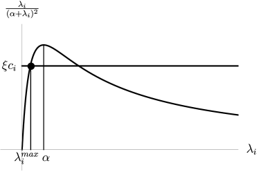
Figure 3.1. Spectral distribution in (3.9).

Proof.

The condition in (3.9) follows from an application of the Cauchy-Schwarz inequality.

The fact that the solution $\left(\lambda_{i}^{max}\right)$ to (3.9) in fact represents the solution to the optimization (3.8) follows from the observation that the one term in the $l^{2}$ inner product is fixed, so the max in (3.8) is attained when quality holds in the corresponding Cauchy-Schwarz Inequality. Further note that, for every fixed value of the index $i$, (3.9) is simply a quadratic equation (see also 3.1), and the optimal spectral distribution $\left(\lambda_{i}^{max}\right)$ is explicit. The form of the optimal p.d. kernel $K$ then follows by substitution of $\left(\lambda_{i}^{max}\right)$ into (3.5). ∎

Corollary 3.5.

Consider the finite-dimensional case, i.e., $\mu$ is atomic, where $K=\sum_{i=1}^{N}\lambda_{i}e_{i}\left(x\right)e_{i}\left(y\right)$, with $\left\{e_{i}\right\}_{i=1}^{N}$ an ONB in $L^{2}\left(\mu\right)$. Then the optimization problem

$$\left\{\begin{aligned} &\max_{\left(\lambda_{i}\right)}\sum_{i=1}^{N}\frac{\lambda_{i}}{\left(\alpha+\lambda_{i}\right)^{2}}c_{i}\\ &\sum_{i=1}^{N}\lambda_{i}=1,\quad\lambda_{i}\geq 0\\ &\sum_{i=1}^{N}c_{i}=\left\|\varphi\right\|_{L^{2}\left(\mu\right)}^{2},\quad c_{i}:=\left|\left\langle e_{i},\varphi\right\rangle\right|^{2}\geq 0\end{aligned}\right.$$ (3.10)

has solution $\left(\lambda_{i}^{max}\right)$ determined by

$$\left(\alpha-\lambda_{i}^{max}\right)c_{i}=A_{N}\left(\alpha+\lambda_{i}^{max}\right)^{3}.$$ (3.11)

See 3.2.

Moreover, we have

$$\left\|f_{N}^{K}\right\|_{\mathscr{H}_{K}}^{2}=\sum_{i=1}^{N}\frac{\lambda_{i}^{max}}{\left(\alpha+\lambda_{i}^{max}\right)^{2}}c_{i}=\sum_{i=1}^{N}\frac{A_{N}^{2/3}\lambda_{i}^{max}c_{i}^{1/3}}{\left(\alpha-\lambda_{i}^{max}\right)^{2/3}}.$$ (3.12)

Proof.

Let $L$ be the Lagrangian, where

$$L=\sum_{i=1}^{N}\frac{\lambda_{i}}{\left(\alpha+\lambda_{i}\right)^{2}}c_{i}-A_{N}\left(\sum_{i=1}^{N}\lambda_{i}-1\right).$$

Then,

$$\frac{\partial L}{\partial\lambda_{i}}=\frac{\alpha^{2}-\lambda_{i}^{2}}{\left(\alpha+\lambda_{i}\right)^{4}}c_{i}-A_{N}=0$$

$$\Updownarrow$$

$$\left(\alpha-\lambda_{i}\right)c_{i}=A_{N}\left(\alpha+\lambda_{i}\right)^{3}.$$

This yields

$$\left(\alpha+\lambda_{i}\right)^{2}=\frac{\left(\alpha-\lambda_{i}\right)^{2/3}c_{i}^{2/3}}{A_{N}^{2/3}}$$

so that

$$\sum_{i=1}^{N}\frac{\lambda_{i}^{max}}{\left(\alpha+\lambda_{i}^{max}\right)^{2}}c_{i}=\sum_{i=1}^{N}\frac{\lambda_{i}^{max}}{\left(\alpha-\lambda_{i}^{max}\right)^{2/3}c_{i}^{2/3}}A_{N}^{2/3}c_{i}=\sum_{i=1}^{N}\frac{\lambda_{i}^{max}}{\left(\alpha-\lambda_{i}^{max}\right)^{2/3}}A_{N}^{2/3}c_{i}^{1/3}$$

which is (3.12). ∎

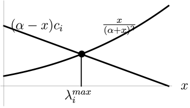
Figure 3.2. The solution $\left(\lambda_{i}^{max}\right)$ determined by the intersection of two curves.

4. Optimization in an ambient Hilbert space

The setting below is as in the previous sections: input is specified by two parts, first a fixed measure $\mu$, and secondly, an input of functions $\varphi$ from $L^{2}\left(\mu\right)$, with the variety of functions representing training data in the model. We then examine optimal choices for p.d. kernels $K$ with view to optimization of $K$-features for the corresponding kernel-learning, see 2 above. The choices of optimal kernels $K$ are made precise in Theorems 3.4, and in 4.4 below. In both cases, an ONB in $L^{2}(\mu)$ is chosen, and we study the corresponding convex sets of Mercer kernels $K$ as specified in (3.5). Here, then each $K$ is determined by a spectral distribution $\left\{\lambda_{i}\right\}$. The corresponding optimization quantity is from (2.2), and it has a $\mathscr{H}_{K}$ penalty term weighted with an assigned parameter $\alpha$, see (2.1). We then arrive at an optimal feature vector $f^{K}$ for every $K$, and we consider its $K$-variance, measured with the use of the $\mathscr{H}_{K}$ norm-squared. Two such variance measures are considered, (3.7) and (4.8). For the first one, we note a singularity blowup for values of $\lambda_{i}$ close to $\alpha$. In the second case, the dependence on $K$ takes a different form; we show that then the $K$-variance (see (4.8)) is monotone, in a sense made precise in 4.4, and 4.5 (spectral a priori error-bounds).

Finally, in 5, we present a solution to the feature optimization with the use of a conditional-mean embedding, CME. The latter refers to (i) a choice of probability space, (ii) a family of p.d. kernels $L$, and corresponding conditional mean embeddings into the RKHSs $\mathscr{H}_{L}$.

Below we first recall some basic facts from operator theory. Let $T:\mathscr{H}_{1}\rightarrow\mathscr{H}_{2}$ be a closed, densely defined linear operator between Hilbert spaces. On $\mathscr{H}_{1}\times\mathscr{H}_{2}$, define the inner product

$$\left\langle\left(u_{1},v_{1}\right),\left(u_{2},v_{2}\right)\right\rangle_{\mathscr{H}_{1}\times\mathscr{H}_{2}}:=\alpha\left\langle u_{1},v_{1}\right\rangle_{\mathscr{H}_{1}}+\left\langle u_{2},v_{2}\right\rangle_{\mathscr{H}_{2}}$$ (4.1)

where $\alpha$ is a positive constant.

Define $W:\mathscr{H}_{1}\rightarrow\mathscr{H}_{1}\times\mathscr{H}_{2}$ by

$$W\left(u\right)=\left(u,Tu\right),\quad u\in dom\left(T\right),$$

Then the projection from $\mathscr{H}_{1}\times\mathscr{H}_{2}$ onto $ran\left(W\right)$ is

$$\begin{bmatrix}\alpha\left(\alpha I_{1}+T^{*}T\right)^{-1}&T^{*}\left(\alpha I_{2}+TT^{*}\right)^{-1}\\ \alpha T\left(\alpha I_{1}+T^{*}T\right)^{-1}&TT^{*}\left(\alpha I_{2}+TT^{*}\right)^{-1}\end{bmatrix}.$$ (4.2)

Remark 4.1.

Recall that in our general setup for regression optimization, we have arranged that training data may be represented via an operator $T$ in Hilbert space. Note that, if $\alpha=1$, then the block matrix in (4.2) represents the projection from the direct sum $\mathscr{H}_{1}\oplus\mathscr{H}_{2}$ onto the graph of the operator $T$, see e.g., [JT21b, Corollary 1.55].

Corollary 4.2.

Let $T:\mathscr{H}_{1}\rightarrow\mathscr{H}_{2}$ be as above. Then, for all $v\in\mathscr{H}_{2}$, we have

$$u^{*} =\mathbb{\text{argmin}}\left\{\alpha\left\|u\right\|_{\mathscr{H}_{1}}^{2}+\left\|Tu-v\right\|_{\mathscr{H}_{2}}^{2}:u\in\mathscr{H}_{1}\right\}$$

$$=\mathop{\text{argmin}}\left\{\left\|Wu-\left(0,v\right)\right\|_{\mathscr{H}_{1}\times\mathscr{H}_{2}}:u\in\mathscr{H}_{1}\right\}$$

$$=T^{*}\left(\alpha I_{2}+TT^{*}\right)^{-1}v.$$ (4.3)

Proof.

Note that

$$\alpha\left\|u\right\|_{\mathscr{H}_{1}}^{2}+\left\|Tu-v\right\|_{\mathscr{H}_{2}}^{2}=\left\|Wu-\left(0,v\right)\right\|_{\mathscr{H}_{1}\times\mathscr{H}_{2}}$$

and the projection of $\left(0,v\right)$ onto $ran\left(W\right)$ is

$$\left(T^{*}\left(\alpha I_{2}+TT^{*}\right)^{-1}v,TT^{*}\left(\alpha I_{2}+TT^{*}\right)^{-1}\right)$$

which is equal to $Wu^{*}=\left(u^{*},Tu^{*}\right)$, for a unique $u^{*}$ in $\mathscr{H}_{1}$. This gives (4.3). ∎

Now, return to optimal feature selections. Fix $\mu$, and consider kernels $K\in\mathscr{K}\left(\mu\right)$, see 2.4. Let $W_{K}:\mathscr{H}_{K}\rightarrow\mathscr{H}_{K}\times L^{2}\left(\mu\right)$, by

$$W_{K}h=\left(h,T_{K,\mu}h\right).$$

The inner product on $\mathscr{H}_{K}\times L^{2}\left(\mu\right)$ is as in (4.1), with parameter $\alpha>0$.

Fix $\varphi\in L^{2}\left(\mu\right)$, then we get a unique $f^{\varphi,K}\in\mathscr{H}_{K}$, such that $W_{K}f^{\varphi,K}$ is the projection of $\left(0,\varphi\right)\in\mathscr{H}_{K}\times L^{2}\left(\mu\right)$ onto $ran\left(W_{K}\right)$. That is,

$$f^{\varphi,K}=T_{K,\mu}^{*}\left(\alpha I_{L^{2}}+T_{K,\mu}T_{K,\mu}^{*}\right)^{-1}\varphi$$ (4.4)

by 4.2.

This motivates the optimization problem:

$$\max_{K\in\mathscr{K}\left(\mu\right)}\left\{\left\|W_{K}f^{\varphi,K}\right\|_{\mathscr{H}_{K}\times L^{2}\left(\mu\right)}^{2}\right\}$$

$$\Updownarrow$$

$$\max_{K\in\mathscr{K}\left(\mu\right)}\left\{\alpha\left\|f^{\varphi,K}\right\|_{\mathscr{H}_{K}}^{2}+\left\|T_{K,\mu}f^{\varphi,K}\right\|_{L^{2}\left(\mu\right)}^{2}\right\}$$

Below is a modification of 3.1.

Lemma 4.3.

With $\mu,K$ fixed, $K\in\mathscr{K}\left(\mu\right)$. Let $f^{\varphi,K}$ be as specified above. Then

$$\left\|W_{K}f^{\varphi,K}\right\|_{\mathscr{H}_{K}\times L^{2}\left(\mu\right)}^{2}=\int\frac{x}{\alpha+x}\left\|Q^{\mu,K}\left(dx\right)\varphi\right\|_{L^{2}\left(\mu\right)}^{2},$$ (4.5)

where $Q^{K,\mu}\left(dx\right)$ is the spectral projection of the operator $T_{K,\mu}T_{K,\mu}^{*}$.

Especially,

$$\left\|W_{K}f^{\varphi,K}\right\|_{\mathscr{H}_{K}\times L^{2}\left(\mu\right)}^{2}\leq\left\|\varphi\right\|_{L^{2}\left(\mu\right)}^{2}.$$ (4.6)

Proof.

Let $T:=T_{K,\mu}$, then

$$\left\|W_{K}f^{\varphi,K}\right\|_{\mathscr{H}_{K}\times L^{2}\left(\mu\right)}^{2} =\alpha\left\|f^{\varphi,K}\right\|_{\mathscr{H}_{K}}^{2}+\left\|Tf^{\varphi,K}\right\|_{L^{2}\left(\mu\right)}^{2}$$

$$=\alpha\left\|T^{*}\left(\alpha+TT^{*}\right)^{-1}\varphi\right\|_{\mathscr{H}_{K}}^{2}+\left\|\left(\alpha+TT^{*}\right)^{-1}TT^{*}\varphi\right\|_{L^{2}\left(\mu\right)}^{2}$$

$$=\int\left(\frac{\alpha x}{\left(\alpha+x\right)^{2}}+\frac{x^{2}}{\left(\alpha+x\right)^{2}}\right)\left\|Q^{\mu,K}\left(dx\right)\varphi\right\|_{L^{2}\left(\mu\right)}^{2}$$

$$=\int\frac{x}{\alpha+x}\left\|Q^{\mu,K}\left(dx\right)\varphi\right\|_{L^{2}\left(\mu\right)}^{2}.$$

Note, (4.6) holds, since $W_{K}f^{\varphi,K}$ is the projection of $\left(0,\varphi\right)\in\mathscr{H}_{K}\times L^{2}\left(\mu\right)$ onto the range of $W$. ∎

Now we state an analog of 3.4.

Theorem 4.4.

Fix $\mu$, and let $K\in\mathscr{K}\left(\mu\right)$. Let $\left\{e_{i}\right\}_{i\in\mathbb{N}}$ be an ONB in $L^{2}\left(\mu\right)$, and consider the p.d. kernel

$$K\left(x,y\right)=\sum\lambda_{i}e_{i}\left(x\right)e_{i}\left(y\right)$$ (4.7)

with $\lambda_{i}>0$.

Let $f^{\varphi,K}$ be the optimal solution as in (4.4). Then,

$$\left\|W_{K}f^{\varphi,K}\right\|_{\mathscr{H}_{K}\times L^{2}\left(\mu\right)}^{2}=\sum\frac{\lambda_{i}}{\alpha+\lambda_{i}}\left|\left\langle\varphi,e_{i}\right\rangle\right|^{2}.$$ (4.8)

Proof.

See the proof of 3.4. ∎

Corollary 4.5.

Let $W_{K}$ and $f^{\varphi,K}$ be as in 4.4, and assume $K$ is bounded. Let $\lambda_{-}=\inf\left\{\lambda_{i}\right\}$, $\lambda_{+}=\sup\left\{\lambda_{i}\right\}$.

1. The following hold:

   $$\frac{\lambda_{-}}{\alpha+\lambda_{-}}\left\|\varphi\right\|_{L^{2}\left(\mu\right)}^{2}\leq\left\|W_{K}f^{\varphi,K}\right\|_{\mathscr{H}_{K}\times L^{2}\left(\mu\right)}^{2}\leq\frac{\lambda_{+}}{\alpha+\lambda_{+}}\left\|\varphi\right\|_{L^{2}\left(\mu\right)}^{2}.$$ (4.9)

2. Equivalently, the approximation error satisfies

   $$\frac{1}{\alpha+\lambda_{+}}\left\|\varphi\right\|_{L^{2}\left(\mu\right)}^{2}\leq err\leq\frac{1}{\alpha+\lambda_{-}}\left\|\varphi\right\|_{L^{2}\left(\mu\right)}^{2}.$$ (4.10)

3. By increasing $\lambda_{-}$, $W_{K}f^{\varphi,K}$ approximates $\left(0,\varphi\right)$ in $\mathscr{H}_{K}\times L^{2}\left(\mu\right)$ arbitrarily well.

Proof.

Notice that the function $f\left(x\right)=\frac{x}{\alpha+x}$ in (4.5) is strictly increasing in $(0,\infty)$, so that (4.9) follows from (4.8). The other assertions are immediate. ∎

Remark 4.6.

The difference between the two feature selection methods in Sections 3 and 4 is as follows.

Fix a measure $\mu$ , and consider $K\in\mathscr{K}\left(\mu\right)$, i.e., all admissible kernels. Let $\mathscr{H}_{K}$ be the associated RKHS. In both cases, for a given $\varphi\in L^{2}\left(\mu\right)$, the best feature vector in $\mathscr{H}_{K}$ is the same

$$f^{K,\varphi}=T_{K}^{*}\left(\alpha+T_{K}T_{K}^{*}\right)^{-1}\varphi.$$

See (2.2) and (4.4).

However, the criteria for optimization over kernels $K$ is different:

Section 3 $$\max_{K\in\mathscr{K}\left(\mu\right)}\left\{\left\|f^{K,\varphi}\right\|_{\mathscr{H}_{K}}^{2}\right\}$$ (4.11)

Section 4 $$\max_{K\in\mathscr{K}\left(\mu\right)}\left\{\alpha\left\|f^{K,\varphi}\right\|_{\mathscr{H}_{K}}^{2}+\left\|T_{K}f^{K,\varphi}\right\|_{L^{2}}^{2}\right\}$$ (4.12)

As discussed at the beginning of (4), the vector

$$\left(f^{K,\varphi},T_{K}f^{K,\varphi}\right)$$

is the projection of $\left(0,\varphi\right)$ in $\mathscr{H}_{K}\times L^{2}$ onto the graph of $T_{K}$. Thus, (4.12) is the norm squared of the projected vector and the corresponding optimization makes use of Hilbert space geometry.

5. Applications to CME

A key feature in what is called conditional mean embedding (CME) concern an analysis of systems of random variable, and conditional distributions, which take values in suitable choices of reproducing kernel Hilbert space, typically infinite-dimensional RKHSs. Hence conditional expectations, and relative transition operators, will entail choices of p.d. kernels, typical one for each random variable under consideration. The implementation of kernel embedding of distributions (also called the kernel mean or mean map) yields nonparametric outcomes in which a probability distribution is represented as an element of a reproducing kernel Hilbert space (RKHS). In diverse applications, the use of CMEs has served as useful tools in for example, problems of sequentially optimizing conditional expectations for objective functions. In such settings, typically both the conditional distribution and the objective function, while fixed, are assumed to be unknown.

The assumption is that input is fixed in the form of a pair $\varphi$ (generalized training data) and $\mu$ as described. The interpretation for feature selection is that variation of choices of p.d. kernels $K$ amounts to a more versatile feature selection. A possible condition on a “good” kernel $K$ is that it will yield optimal selection of feature function $f^{K}$, i.e., representing an output of more distinct features. Often a feature functions $f^{K}$ with large $\mathscr{H}_{K}$-norm² comes from a choice of $K$ that yields a more successful discrimination by features that reflects input of training data via $\varphi$. More precisely, the $\mathscr{H}_{K}$-norm² refers to the features selected with optimal choices of $K$.

The setting for CME is as follows:

Let $X,Y$ be random variables on a probability space $\left(\Omega,\mathscr{C},\mathbb{P}\right)$, taking values in sets $A,B$, respectively, and has joint measure

$$\mu\left(S_{1}\times S_{1}\right)=\mathbb{P}\left(X^{-1}\left(S_{1}\right)\cap Y^{-1}\left(S_{2}\right)\right)$$

for all $S_{1}\times S_{2}\subset A\times B$.

Denote by $\mu_{X},\mu_{Y}$ the corresponding marginal measures, and let $\mu_{Y\mid x}$ be the conditional measure defined as

$$\mu_{Y\mid x}\left(S\right)=\mathbb{P}\left(Y^{-1}\left(S\right)\mid X=x\right)$$

for all $S\subset B$ and $x\in A$.

Assume further that $K,L$ are given p.d. kernels on $A$, $B$ with RKHSs $\mathscr{H}_{K}$, $\mathscr{H}_{L}$, respectively.

Lemma 5.1.

For every $x\in A$, set

$$\pi\left(x\right):=\mathbb{E}\left[L\left(\cdot,Y\right)\mid X=x\right]=\int L\left(\cdot,y\right)d\mu_{Y\mid x}\left(y\right)$$ (5.1)

Then, for all $f\in\mathscr{H}_{L}$, it holds that

$$\left\langle\pi\left(x\right),f\right\rangle_{\mathscr{H}_{L}}=\int\left\langle L\left(\cdot,y\right),f\right\rangle d\mu_{Y\mid x}\left(y\right)=\mathbb{E}\left[f\left(Y\right)\mid X=x\right].$$ (5.2)

The map $x\mapsto\pi\left(x\right)$ is called the kernel mean embedding (KME) of the conditional expectation $\mathbb{E}\left[\;\cdot\mid X=x\right]$.

Remark 5.2.

Note that the integral on the RHS in formula (5.1) is an extension of (2.8) from 2.5 above. Moreover, the proof of the lemma follows the ideas in 2.

Lemma 5.3.

As in 5.1, consider $\pi\left(x\right)$ for $x\in A$, as per the definition (5.1) in 5.1. Then

1. $\pi\left(x\right)\in\mathscr{H}_{L}$ if and only if

   $$\mathbb{E}\left[L\left(Y,Y\right)\mid X=x\right]:=\mu_{Y\mid x}L\mu_{Y\mid x}<\infty,$$ (5.3)

   where

   $$\mu_{Y\mid x}L\mu_{Y\mid x}=\iint L\left(y_{1},y_{2}\right)d\mu_{Y\mid x}\left(y_{1}\right)d\mu_{Y\mid x}\left(y_{2}\right).$$

2. $\pi\in L^{2}\left(A,\mu_{X}\right)\otimes\mathscr{H}_{L}$ if and only if

   $$\mathbb{E}\left[K\left(Y,Y\right)\right]=\int\left(\mu_{Y\mid x}L\mu_{Y\mid x}\right)d\mu_{X}\left(x\right)<\infty.$$

   In that case, setting $\widetilde{\pi}\left(f\right)\left(x\right):=\left\langle\pi\left(x\right),f\right\rangle_{\mathscr{H}_{L}}$, then

   $$\int\left\|\widetilde{\pi}\left(f\right)\right\|_{\mathscr{H}_{K}}^{2}d\mu_{X}\leq\mathbb{E}\left[K\left(Y,Y\right)\right]\left\|f\right\|_{\mathscr{H}_{L}}^{2}$$

   for all $f\in\mathscr{H}_{L}$.

Proof.

Consider the filter of finite measurable partitions $\mathscr{P}\left(B\right)$ of the measurable space $\left(B,\mathscr{B}\right)$, i.e., $\left\{A_{i}\right\}_{i=1}^{N}$ for some $N<\infty$, with $A_{i}\in\mathscr{B}$, $A_{i}\cap A_{j}=\emptyset$ if $i\neq j$, and $\cup_{i}A_{i}=B$, then

$$\sum_{i=1}^{N}L\left(\cdot,y_{i}\right)\mu_{Y\mid x}\left(A_{i}\right)\in\mathscr{H}_{K}$$ (5.4)

with

$$\left\|\sum\nolimits_{i=1}^{N}L\left(\cdot,y_{i}\right)\mu_{Y\mid x}\left(A_{i}\right)\right\|_{\mathscr{H}_{K}}^{2}=\sum\nolimits_{i}\sum\nolimits_{j}\mu_{Y\mid x}\left(A_{i}\right)L\left(y_{i},y_{j}\right)\mu_{Y\mid x}\left(A_{j}\right).$$ (5.5)

Since $L$ is assumed measurable, the right-hand side of (5.5) has a limit, as we pass to the limit of the filter of all measurable partitions $\mathscr{P}\left(B\right)$, see (5.4), and the limit is well defined and finite if and only if (5.3) holds. This follows from the following computation:

$$\iint\mu_{Y\mid x}\left(dy_{1}\right)L\left(y_{1},y_{2}\right)\mu_{Y\mid x}\left(dy_{2}\right)=\mathbb{E}\left[L\left(Y,Y\right)\mid X=x\right].$$

But since we have “$=$” in the identity (5.5) for all finite partitions, it follows that (5.3) holds if and only if the integral on the right-hand side in (5.1) is convergent with its values in $\mathscr{H}_{L}$.

The second part of the lemma is immediate. ∎

Remark 5.4.

The setting of the lemma is a fixed a p.d. kernel $L$ and a measure space $\left(B,\mathscr{B}\right)$. We have $L$ defined on $B\times B$ and assumed measurable w.r.t. the corresponding product sigma algebra. The key idea behind the justification of the RKHS $\mathscr{H}_{L}$ valued integral $\pi(x)$ in (5.1) is a rigorous justification of a limit of an approximation by finite sums in $\mathscr{H}_{L}$, and the limit with respect to the RKHS norm in $\mathscr{H}_{L}$. This is doable as per our discussion, but the limit will be indexed by a filter of partitions of the measure space $\left(B,\mathscr{B}\right)$. And the limit is with respect to refinement within the filter of partitions, where refinement defined by recursive subdivision, i.e., subdivisions of one partition are creating a finer partition. Note that the reasoning involves the same kind of limit which is used in the justification of general Ito isometries, and Ito integrals for Gaussian processes.

Question 5.5.

Assume $\pi\in L^{2}\left(A,\mu_{X}\right)\otimes\mathscr{H}_{L}$. What is the best approximation to choice of CME $\mu$ from an $\mathscr{H}_{L}$-valued RKHS?

One option in the literature is to approximate $\pi$ from $\mathscr{H}_{K}\otimes\mathscr{H}_{L}$. More generally, one may start from an $\mathscr{B}\left(\mathscr{H}_{L}\right)$-valued p.d. kernel $S:A\times A\rightarrow\mathscr{B}\left(\mathscr{H}_{L}\right)$, i.e.,

$$\sum_{i,j=1}^{N}\left\langle u_{i},S\left(x_{i},x_{j}\right)u_{j}\right\rangle_{\mathscr{H}_{L}}\geq 0$$ (5.6)

$\forall\left(x_{i}\right)_{i=1}^{N}\subset A$, $\forall\left(u_{i}\right)_{i=1}^{N}\subset\mathscr{H}_{L}$, and $\forall N\in\mathbb{N}$.

Let $\mathscr{H}_{S}$ be the Hilbert completion of the set $span\left\{S\left(\cdot,x\right)u:x\in A,u\in\mathscr{H}_{L}\right\}$ with respect to the inner product

$$\left\langle\sum S\left(\cdot,x_{i}\right)u_{i},\sum S\left(\cdot,x_{j}\right)v_{j}\right\rangle_{\mathscr{H}_{S}}:=\sum_{i,j}\left\langle u_{i},S\left(x_{i},x_{j}\right)v_{j}\right\rangle_{\mathscr{H}_{L}}.$$ (5.7)

Then $\mathscr{H}_{S}$ is an RKHS with the following reproducing property:

For all $F\in\mathscr{H}_{S}$, $x\in A$ and $u\in\mathscr{H}_{L}$, we have

$$\left\langle u,F\left(x\right)\right\rangle_{\mathscr{H}_{L}}=\left\langle S\left(\cdot,x\right)u,F\right\rangle_{\mathscr{H}_{L}}.$$ (5.8)

Remark 5.6.

In the special case $\mathscr{H}_{S}=\mathscr{H}_{K}\otimes\mathscr{H}_{L}$, we have $S\left(x,y\right)=K\left(x,y\right)I_{\mathscr{H}_{L}}$, where $K$ is the scalar valued p.d. kernel of $\mathscr{H}_{K}$, and $I_{\mathscr{H}_{L}}$ denotes the identity operator on $\mathscr{H}_{L}$.

Theorem 5.7.

Assume $S$ is compatible with the marginal distribution of $X$, then we have

$$f^{\pi,S} :=\mathop{\text{argmin}}\left\{\left\|T_{S}f-\pi\right\|_{L^{2}\left(A\right)\otimes\mathscr{H}_{L}}^{2}+\alpha\left\|f\right\|_{\mathscr{H}_{S}}^{2}\right\}$$ (5.9)

$$=T_{S}^{*}\left(\alpha+T_{S}T_{S}^{*}\right)^{-1}\pi.$$ (5.10)

Then, we may apply the methods from 3 to the problem:

$$\max_{S}\left\|f^{\pi,S}\right\|_{\mathscr{H}_{S}}^{2}.$$ (5.11)

Proof.

Illustrating the versatility of Hilbert space operators, the reader will be able to fill in the argument for this formula (5.10), and its implications, following the general framework presented in sections 2 and 3 above. ∎

6. A new convex set of p.d. kernels

Let $\mathcal{M}\left(\mathbb{R}\right)$ be the set of all Borel measures on $\mathbb{R}$, and $\mathcal{M}_{1}\left(\mathbb{R}\right)$ be the subset of probability measures. For all $\rho\in\mathcal{M}\left(\mathbb{R}\right)$, let

$$\widehat{\rho}\left(\xi\right)=\int_{\mathbb{R}}e^{i\xi x}d\rho\left(x\right)$$ (6.1)

denote the Fourier transform.

Consider the following convex set of stationary kernels

$$G_{1}=\left\{\mathbb{R}\times\mathbb{R}\xrightarrow{\;K_{g}\;}\mathbb{C}:K_{g}\left(x,y\right)=g\left(x-y\right),\;g=\widehat{\mu},\>\mu\in\mathcal{M}_{1}\left(\mathbb{R}\right)\right\}.$$ (6.2)

Lemma 6.1.

Fix $K_{g}\in G_{1}$, and let $\mathscr{H}_{K_{g}}$ be the corresponding RKHS. Then, for all $\rho\in\mathcal{M}\left(\mathbb{R}\right)$,

$$g\ast d\rho:=\int_{\mathbb{R}}K_{g}\left(\cdot,y\right)d\rho\left(y\right)\in\mathscr{H}_{K_{g}}$$ (6.3)

$$\Updownarrow$$

$$\int_{\mathbb{R}}\left|\widehat{\rho}\left(\xi\right)\right|^{2}d\mu\left(\xi\right)<\infty.$$ (6.4)

Proof.

Assume $g\ast d\rho\in\mathscr{H}_{K_{g}}$, then

$$\left\|g\ast d\rho\right\|_{\mathscr{H}_{K_{g}}}^{2} =\iint\left\langle K_{g}\left(\cdot,y\right),K_{g}\left(\cdot,z\right)\right\rangle_{\mathscr{H}_{K_{g}}}d\rho\left(y\right)d\rho\left(z\right)$$

$$=\iint g\left(y-z\right)d\rho\left(y\right)d\rho\left(z\right)$$

$$=\int\left(\iint e^{i\xi\left(y-z\right)}d\rho\left(y\right)d\rho\left(z\right)\right)d\mu\left(\xi\right)$$

$$=\int\left|\widehat{\rho}\left(\xi\right)\right|^{2}d\mu\left(\xi\right)<\infty.$$

Conversely, suppose $C:=\int\left|\widehat{\rho}\left(\xi\right)\right|^{2}d\mu\left(\xi\right)<\infty$. Then, for all $\sum c_{k}K_{g}\left(\cdot,x_{k}\right)$, we have

$$\sum c_{k}K_{g}\left(\cdot,x_{k}\right) \longmapsto \left|\sum c_{k}\left(g\ast d\rho\right)\left(x_{k}\right)\right|^{2}$$

$$= \left|\sum c_{k}\int\int e^{i\xi\left(x_{k}-y\right)}d\rho\left(y\right)d\mu\left(\xi\right)\right|^{2}$$

$$\leq \int\left|\sum c_{k}e^{i\xi x_{k}}\right|\left|\widehat{\rho}\left(\xi\right)\right|d\mu\left(\xi\right)^{2}$$

$$\leq \int\left|\sum c_{k}e^{i\xi x_{k}}\right|^{2}d\mu\left(\xi\right)\int\left|\widehat{\rho}\left(\xi\right)\right|^{2}d\mu\left(\xi\right)$$

$$= C\cdot\sum_{k}\sum_{l}\overline{c_{k}}c_{l}K_{g}\left(x_{k},x_{l}\right).$$

It follows that $g\ast d\rho\in\mathscr{H}_{K_{g}}$ by density and Riesz’s theorem. ∎

Fix $K_{g}\in G_{1}$, and let $\mathscr{H}_{K_{g}}$ be the RKHS. Let $d\lambda$ denote the Lebesgue measure on $\mathbb{R}$. Suppose $\left\{\varphi\in L^{2}\left(d\lambda\right):\widehat{\varphi}\in L^{2}\left(\mu\right)\right\}$ is dense in $L^{2}\left(d\lambda\right)$. Then, the operator

$$T_{\lambda}:\mathscr{H}_{K_{g}}\rightarrow L^{2}\left(d\lambda\right),\quad T_{\lambda}\left(\sum_{i}c_{i}K_{g}\left(\cdot,x_{i}\right)\right)=\sum_{i}c_{i}K_{g}\left(\cdot,x_{i}\right)$$ (6.5)

is densely defined and closable, and its adjoint is given by

$$T_{\lambda}^{*}:L^{2}\left(d\lambda\right)\rightarrow\mathscr{H}_{K_{g}},\quad T_{\lambda}^{*}\left(\varphi\right)=g\ast\varphi,\;\forall\varphi\in dom\left(T_{\lambda}^{*}\right)$$ (6.6)

where $dom\left(T_{\lambda}^{*}\right)=\left\{\varphi\in L^{2}\left(d\lambda\right):\widehat{\varphi}\in L^{2}\left(\mu\right)\right\}$.

Corollary 6.2.

For all $\varphi\in dom\left(T_{\lambda}^{*}\right)$, we have

$$\left\|T_{\lambda}^{*}\varphi\right\|_{\mathscr{H}_{K_{g}}}^{2}=\int\left|\widehat{\varphi}\left(\xi\right)\right|^{2}d\mu\left(\xi\right).$$ (6.7)

Proof.

This follows from 6.1 by setting $d\rho=gd\lambda$, and $\widehat{\varphi}$ is the $L^{2}$-Fourier transform of $\varphi$. ∎

Example 6.3.

Consider the following two p.d. kernels on $\mathbb{R}$:

$$K_{1}\left(x,y\right)=e^{-\left|x-y\right|},\quad,K_{2}\left(x,y\right)=e^{-\frac{1}{2}\left(x-y\right)^{2}}.$$ (6.8)

Note that

$$g_{1}\left(x\right) =e^{-\left|x\right|}=\int e^{i\xi x}d\mu_{1}\left(\xi\right)\quad d\mu_{1}\left(\xi\right)=\frac{1}{\pi}\frac{1}{1+\xi^{2}}d\xi,$$

$$g_{2}\left(x\right) =e^{-\frac{1}{2}x^{2}}=\int e^{i\xi x}d\mu_{2}\left(\xi\right)\quad d\mu_{2}\left(\xi\right)=\frac{1}{\sqrt{2\pi}}e^{-\frac{1}{2}\xi^{2}}d\xi.$$

Moreover, for $K_{1}$, if $\varphi\in L^{2}\left(\mathbb{R}\right)$, then

$$\left\|g_{1}\ast\varphi\right\|_{\mathscr{H}_{K_{1}}}^{2}=\int_{\mathbb{R}}\frac{\left|\widehat{\varphi}\left(\xi\right)\right|^{2}d\xi}{1+\xi^{2}}=\left\langle\varphi,\left(1-\left(d/dx\right)^{2}\right)^{-1}\varphi\right\rangle_{L^{2}\left(\mathbb{R}\right)}.$$

In other words, the RKHS is the RKHS from the Green’s function for $1-\left(d/dx\right)^{2}$, or $1-\Delta$ in $\mathbb{R}^{n}$, $n>1$.

Given $K_{g}\in G_{1}$, the convolution $\varphi\mapsto g\ast\varphi\in\mathscr{H}_{K_{g}}$ may be extended to measures or distributions.

Lemma 6.4.

Let $K_{g}\in G_{1}$, and $\mathscr{H}_{K_{g}}$ be the corresponding RKHS. Then,

$$g\left(x-\cdot\right)=g\ast\delta_{x}\in\mathscr{H}_{K_{g}}$$ (6.9)

and

$$g\ast\delta^{\prime}_{x}\in\mathscr{H}_{K_{g}}\Longleftrightarrow\int\left|\xi\right|^{2}\mu\left(d\xi\right)<\infty.$$ (6.10)

Note (6.10) is satisfied for $K_{2}$ but not for $K_{1}$ in 6.3.

Proof.

Using $g\ast\delta_{x}=g\left(x-\cdot\right)$, we have $g\ast\delta_{x}\in\mathscr{H}_{K_{g}}$ and

$$\left\|g\left(x-\cdot\right)\right\|_{\mathscr{H}_{K_{g}}}^{2}=\left\langle g\left(x-\cdot\right),g\left(x-\cdot\right)\right\rangle_{\mathscr{H}_{K_{g}}}=g\left(x-x\right)=g\left(0\right)=1.$$

Equivalently, $\delta_{x}\leftrightarrow\widehat{\delta}_{x}\left(\xi\right)=e^{i\xi x}$, $\xi\in\mathbb{R}$, and

$$\int|\widehat{\delta_{x}}|^{2}d\mu=\int\left|e^{ix\xi}\right|^{2}\mu\left(d\xi\right)=\mu\left(\mathbb{R}\right)=g\left(0\right)=1.$$

Similarly, $\delta^{\prime}_{x}\leftrightarrow\widehat{\delta^{\prime}_{x}}\left(\xi\right)=i\xi e^{ix\xi}$. Thus $g\ast\delta^{\prime}_{x}\in\mathscr{H}_{K_{g}}$ if and only if $\int\left|\xi\right|^{2}\mu\left(d\xi\right)<\infty$. ∎

Remark 6.5.

Given $K_{g}\left(x,y\right)=g\left(x-y\right)$, where $g\left(x\right)=\int e^{i\xi x}\mu\left(d\xi\right)$, and $\mu$ is a finite positive Borel measure on $\mathbb{R}$, the reproducing property of $\mathscr{H}_{K_{g}}$ below may be verified using Fourier-inversion:

$$\left\langle g\left(x-\cdot\right),\varphi\ast g\right\rangle_{\mathscr{H}_{K}}=\left(\varphi\ast g\right)\left(x\right),\;\forall x\in\mathbb{R}.$$

Proof.

Indeed, we have

$$\left\langle g\left(x-\cdot\right),\varphi\ast g\right\rangle_{\mathscr{H}_{K}} =\int\overline{e^{i\xi x}}\widehat{\varphi}\left(\xi\right)\mu\left(d\xi\right)$$

$$=\int_{\mathbb{R}}e^{i\xi x}\widehat{\varphi\ast g}\left(\xi\right)d\xi=\left(\varphi\ast g\right)\left(x\right).$$

∎

Theorem 6.6.

Fix $K_{g}\in G_{1}$, and let $\mathscr{H}_{K_{g}}$ be the RKHS. Let $T_{\lambda}:\mathscr{H}_{K_{g}}\rightarrow L^{2}\left(d\lambda\right)$ be as in (6.5), where $d\lambda$ denotes the Lebesgue measure on $\mathbb{R}$. Let $f^{g,\lambda}$ be the solution in 2.2, i.e.,

$$f^{g,\lambda}=T_{\lambda}^{*}\left(\alpha+T_{\lambda}T_{\lambda}^{*}\right)^{-1}\varphi$$ (6.11)

where $\varphi\in L^{2}\left(d\lambda\right)$ is fixed. Then, by the $L^{2}$-Fourier transform, we have

$$\widehat{T_{\lambda}f^{g,\lambda}}=\left[T_{\lambda}T_{\lambda}^{*}\left(\alpha+T_{\lambda}T_{\lambda}^{*}\right)^{-1}\varphi\right]^{\wedge}=\frac{\widehat{g}}{\alpha+\widehat{g}}\widehat{\varphi}.$$ (6.12)

Moreover, the optimal selections from 3.1 and 4.3, respectively, admit the following explicit spectral representations:

$$\left\|f^{g,\lambda}\right\|_{\mathscr{H}_{K_{g}}}^{2} =\int\frac{\widehat{g}\left(\lambda\right)}{\left(\alpha+\widehat{g}\left(\lambda\right)\right)^{2}}\left|\widehat{\varphi}\left(\lambda\right)\right|^{2}d\lambda$$ (6.13)

$$\left\|W_{K_{g}}f^{g,\lambda}\right\|_{\mathscr{H}_{K_{g}}\times L^{2}\left(d\lambda\right)}^{2} =\int\frac{\widehat{g}\left(\lambda\right)}{\alpha+\widehat{g}\left(\lambda\right)}\left|\widehat{\varphi}\left(\lambda\right)\right|^{2}d\lambda$$ (6.14)

Proof.

By the definition of $T_{\lambda}^{*}$ from (6.6), it follows that $T_{\lambda}T_{\lambda}^{*}\varphi=g\ast\varphi\in L^{2}\left(d\lambda\right)$, and so $\widehat{T_{\lambda}T_{\lambda}^{*}\varphi}=\widehat{g}\widehat{\varphi}$.

It follows from this, that

$$\left\|f^{g,\lambda}\right\|_{\mathscr{H}_{K_{g}}}^{2} \underset{\left(\ref{eq:C2}\right)}{=} \left\|\left(T_{\lambda}T_{\lambda}^{*}\right)^{1/2}\left(\alpha+T_{\lambda}T_{\lambda}^{*}\right)^{-1}\varphi\right\|_{L^{2}\left(d\lambda\right)}^{2}$$

$$= \int\frac{\widehat{g}\left(\lambda\right)}{\left(\alpha+\widehat{g}\left(\lambda\right)\right)^{2}}\left|\widehat{\varphi}\left(\lambda\right)\right|^{2}d\lambda$$

and on the other hand,

$$\left\|W_{K_{g}}f^{g,\lambda}\right\|_{\mathscr{H}_{K_{g}}\times L^{2}\left(d\lambda\right)}^{2} \underset{\left(\ref{eq:d11}\right)}{=} \left\langle\varphi,T_{\lambda}T_{\lambda}^{*}\left(\alpha+T_{\lambda}T_{\lambda}^{*}\right)^{-1}\varphi\right\rangle_{L^{2}\left(d\lambda\right)}$$

$$= \int\frac{\widehat{g}\left(\lambda\right)}{\alpha+\widehat{g}\left(\lambda\right)}\left|\widehat{\varphi}\left(\lambda\right)\right|^{2}d\lambda.$$

∎

Example 6.7.

Let $K_{1}$ and $K_{2}$ be the p.d. kernels from (6.8). The formulas in (6.13)-(6.14) take explicit forms, summarized in 1.

$K_{g}=g\left(x-y\right)$	$g=\widehat{\mu}$	$\mu$	$\frac{\widehat{g}}{\left(\alpha+\widehat{g}\right)^{2}}$	$\frac{\widehat{g}}{\alpha+\widehat{g}}$
$K_{1}=e^{-\left|x-y\right|}$	$g_{1}=e^{-\left|x\right|}$	$d\mu_{1}=\frac{1}{1+\xi^{2}}d\xi$	$\frac{1+\xi^{2}}{\left(1+\alpha\left(1+\xi^{2}\right)\right)^{2}}$	$\frac{1}{1+\alpha\left(1+\xi^{2}\right)}$
$K_{2}=e^{-\frac{1}{2}\left(x-y\right)^{2}}$	$g_{2}=e^{-\frac{1}{2}x^{2}}$	$d\mu_{2}=e^{-\frac{1}{2}\xi^{2}}d\xi$	$\frac{e^{\frac{1}{2}x^{2}}}{\left(1+\alpha e^{\frac{1}{2}x^{2}}\right)^{2}}$	$\frac{1}{1+\alpha e^{\frac{1}{2}\xi^{2}}}$

Table 1. The p.d. kernels $K_{1}$ and $K_{2}$.

References

[CnBCFR21]
Juan Cerviño, Juan Andrés Bazerque, Miguel Calvo-Fullana, and Alejandro
Ribeiro, Multi-task reinforcement learning in reproducing kernel
Hilbert spaces via cross-learning, IEEE Trans. Signal Process. 69
(2021), 5947–5962. MR 4341244
[GLB+12]
Steffen Grünewälder, Guy Lever, Luca Baldassarre, Sam Patterson, Arthur
Gretton, and Massimilano Pontil, Conditional mean embeddings as
regressors, Proceedings of the 29th International Coference on International
Conference on Machine Learning (Madison, WI, USA), ICML’12, Omnipress, 2012,
pp. 1803–1810.
[JST21]
Palle E. T. Jorgensen, Myung-Sin Song, and James Tian, Positive definite
kernels, algorithms, frames, and approximations, 2021.
[JT19a]
Palle Jorgensen and Feng Tian, Decomposition of Gaussian processes, and
factorization of positive definite kernels, Opuscula Math. 39
(2019), no. 4, 497–541. MR 3964760
[JT19b]
by same author, Realizations and factorizations of positive definite kernels,
J. Theoret. Probab. 32 (2019), no. 4, 1925–1942. MR 4020693
[JT20]
Palle Jorgensen and James Tian, Sampling with positive definite kernels
and an associated dichotomy, Adv. Theor. Math. Phys. 24 (2020),
no. 1, 125–154. MR 4106884
[JT21a]
by same author, Reproducing kernels: harmonic analysis and some of their
applications, Appl. Comput. Harmon. Anal. 52 (2021), 279–302.
MR 4218424
[JT22]
by same author, Reproducing kernels and choices of associated feature spaces, in
the form of -spaces, J. Math. Anal. Appl. 505 (2022), no. 2,
Paper No. 125535, 31. MR 4295177
[KSS20]
Ilja Klebanov, Ingmar Schuster, and T. J. Sullivan, A rigorous theory of
conditional mean embeddings, SIAM J. Math. Data Sci. 2 (2020),
no. 3, 583–606. MR 4121886
[LMY16]
Yeon Ju Lee, Charles A. Micchelli, and Jungho Yoon, On multivariate
discrete least squares, J. Approx. Theory 211 (2016), 78–84.
MR 3547633
[LRI21]
David K. Lim, Naim U. Rashid, and Joseph G. Ibrahim, Model-based feature
selection and clustering of RNA-seq data for unsupervised subtype
discovery, Ann. Appl. Stat. 15 (2021), no. 1, 481–508.
MR 4255285
[LS21]
Chi-Ken Lu and Patrick Shafto, Conditional Deep Gaussian Processes:
Multi-Fidelity Kernel Learning, Entropy 23 (2021), no. 11,
Paper No. 1545. MR 4349381
[LSTSS16]
Guy Lever, John Shawe-Taylor, Ronnie Stafford, and Csaba Szepesvári,
Compressed conditional mean embeddings for model-based reinforcement
learning, AAAI, 2016, pp. 1779–1787.
[LZW21]
Tingyu Lai, Zhongzhan Zhang, and Yafei Wang, A kernel-based measure for
conditional mean dependence, Comput. Statist. Data Anal. 160
(2021), Paper No. 107246, 22. MR 4242933
[LZWK21]
Tingyu Lai, Zhongzhan Zhang, Yafei Wang, and Linglong Kong, Testing
independence of functional variables by angle covariance, J. Multivariate
Anal. 182 (2021), Paper No. 104711, 15. MR 4187269
[MGP21]
Erfan Mehmanchi, Andrés Gómez, and Oleg A. Prokopyev, Solving a
class of feature selection problems via fractional 0-1 programming, Ann.
Oper. Res. 303 (2021), no. 1-2, 265–295. MR 4288278
[MPWZ16]
Charles A. Micchelli, Massimiliano Pontil, Qiang Wu, and Ding-Xuan Zhou,
Error bounds for learning the kernel, Anal. Appl. (Singap.)
14 (2016), no. 6, 849–868. MR 3564937
[NSW11]
P. Niyogi, S. Smale, and S. Weinberger, A topological view of
unsupervised learning from noisy data, SIAM J. Comput. 40 (2011),
no. 3, 646–663. MR 2810909
[PM21]
Junhyung Park and Krikamol Muandet, A measure-theoretic approach to
kernel conditional mean embeddings, 2021.
[RCOR20]
Sayak Ray Chowdhury, Rafael Oliveira, and Fabio Ramos, Active learning of
conditional mean embeddings via bayesian optimisation, Proceedings of the
36th Conference on Uncertainty in Artificial Intelligence (UAI) (Jonas Peters
and David Sontag, eds.), Proceedings of Machine Learning Research, vol. 124,
PMLR, 03–06 Aug 2020, pp. 1119–1128.
[SY06]
Steve Smale and Yuan Yao, Online learning algorithms, Found. Comput.
Math. 6 (2006), no. 2, 145–170. MR 2228737
[SZ09]
Steve Smale and Ding-Xuan Zhou, Geometry on probability spaces, Constr.
Approx. 30 (2009), no. 3, 311–323. MR 2558684
[XWCT21]
Ping Xu, Yue Wang, Xiang Chen, and Zhi Tian, COKE:
communication-censored decentralized kernel learning, J. Mach. Learn. Res.
22 (2021), Paper No. 196, 35. MR 4329775
[ZC21]
Yikun Zhang and Yen-Chi Chen, Kernel smoothing, mean shift, and their
learning theory with directional data, J. Mach. Learn. Res. 22
(2021), Paper No. 154, 92. MR 4318510
[ZL21]
Puning Zhao and Lifeng Lai, Minimax rate optimal adaptive nearest
neighbor classification and regression, IEEE Trans. Inform. Theory
67 (2021), no. 5, 3155–3182. MR 4282408