Accelerating genetic optimization of nonlinear model predictive control by learning optimal search space size

Abstract

Nonlinear model predictive control (NMPC) solves a multivariate optimization problem to estimate the system’s optimal control inputs in each control cycle. Such optimization is made more difficult by several factors, such as nonlinearities inherited in the system, highly coupled inputs, and various constraints related to the system’s physical limitations. These factors make the optimization to be non-convex and hard to solve traditionally. Genetic algorithm (GA) is typically used extensively to tackle such optimization in several application domains because it does not involve differential calculation or gradient evaluation in its solution estimation. However, the size of the search space in which the GA searches for the optimal control inputs is crucial for the applicability of the GA with systems that require fast response. This paper proposes an approach to accelerate the genetic optimization of NMPC by learning optimal search space size. The proposed approach trains a multivariate regression model to adaptively predict the best smallest search space in every control cycle. The estimated best smallest size of search space is fed to the GA to allow for searching the optimal control inputs within this search space. The proposed approach not only reduces the GA’s computational time but also improves the chance of obtaining the optimal control inputs in each cycle. The proposed approach was evaluated on two nonlinear systems and compared with two other genetic-based NMPC approaches implemented on the GPU of a Nvidia Jetson TX2 embedded platform in a processor-in-the-loop (PIL) fashion. The results show that the proposed approach provides a 39-53% reduction in computational time. Additionally, it increases the convergence percentage to the optimal control inputs within the cycle’s time by 48-56%, resulting in a significant performance enhancement. The source code is available on GitHub.

I Introduction

Model predictive control (MPC) is a powerful control method used to control a system while satisfying a set of constraints [1]. The MPC method deals with multivariate control problems, i.e., controlling systems with multiple states/control inputs. It generates the optimal control inputs in each control cycle by minimizing a multivariate optimization problem subject to given constraints. The main advantage of the MPC is that it optimizes the current control problem while considering the future. This is achieved by optimizing the control problem in a future time horizon to generate the best control inputs along this horizon.

The multivariate optimization problem of the MPC makes its computational burden challenging, especially when controlling complex or nonlinear systems. Specifically, the optimization problem is made more difficult by nonlinearities, highly coupled inputs, and various constraints related to physical limitations and safety, making the optimization non-convex. This computational burden is highly noticeable, particularly when running the MPC optimization on embedded hardware with limited processing resources.

Several classical optimization solvers have been developed to handle complex MPC optimization problems. These solvers can be linear or nonlinear [2]. The linear solvers assume the system has linear dynamics and constraints. However, these linearity assumptions are only valid for some systems, so nonlinear solvers are needed to accommodate nonlinear dynamics and constraints for most systems. Unfortunately, this comes at the expense of increased computational time, which can be a significant barrier when applying MPC in systems that require fast response, i.e., have short control cycles allowed.

Other optimization solvers use heuristic algorithms like the genetic algorithm (GA) [3]. GA solves the optimization problem by starting with a population of candidate solutions chosen from a specified search space. These solutions are evaluated and crossed over to produce the best optimal solution before the control cycle time expires or a sub-optimal solution if the termination condition is met. The GA offers two main advantages over classical optimization solvers. First, it can solve MPC optimization problems even when the optimization function constitutes non-differential, discontinuous, or nonlinear components since its implementation does not involve differential calculation or gradient evaluation. Specifically, the GA can deal with if/else conditions, trigonometric, piecewise, and other functions, making it suitable for a wide range of optimization problems. The second advantage of the GA is that its implementation can be accelerated by parallelizing its computation on GPUs. These advantages make the GA solver a powerful tool for solving complex optimization problems. However, the size of the search space in which the GA searches for the optimal control inputs is crucial for the applicability of the GA with systems that require fast response. A small search space lowers the probability of finding the optimal control inputs in the current cycle. In contrast, a large search space increases this probability but at the expense of more computations [4, 5, 6]. Thus, wisely limiting the search space can significantly improve the chance of obtaining the optimal control inputs in the current within a shorter computational time.

This paper proposes an approach to accelerate the genetic optimization of nonlinear model predictive control (NMPC) by learning optimal search space size. The proposed approach trains a regression model to adaptively predict the best smallest search space in every control cycle to improve the chance of obtaining the optimal control inputs within the shortest computational time. To achieve this, we first build a synthetic dataset using the system’s model. Then, we train a regressor on the dataset and use the regression model to estimate the best smallest size of the search space. The estimated best smallest size of search space is fed to the GA to allow for searching the optimal control inputs within this search space. To show the effectiveness of the proposed approach in practical scenarios, we implement it on the GPU of a Nvidia^™ Jetson TX2 [7] embedded platform in a processor-in-the-loop (PIL) fashion. Furthermore, the proposed approach was evaluated on two nonlinear systems and compared with two other genetic-based NMPC techniques implemented on the same platform. The proposed approach provides a 39-53% reduction in computational time compared with other techniques while, at the same time, it improves the chance of obtaining the optimal control inputs in each cycle. Specifically, it increases the percentage of convergence to the optimal control inputs within the cycle’s time by 48-56%. The source code of the proposed approach is available online.

The remainder of this paper is organized as follows. Section II presents a short survey of using the GA to tackle the NMPC optimization in various application domains. Section III presents the mathematical formulation of the NMPC and the GA algorithm in detail. In Section IV, we motivate and present the proposed approach for learning the optimal search space size for genetic optimization. Section V presents the experimental setup and discusses the experimental results that evaluate our proposed approach. Section VI summarizes our conclusion and presents our future works.

II Literature survey

Numerous publications have explored using GA to tackle NMPC optimization in various application domains. We can categorize the usage of the GA with NMPC into two research directions. The first direction focused on employing GA to solve the NMPC optimization problem directly in optimal or sub-optimal fashions. The second direction involves leveraging GA to optimize the parameters of the NMPC controller. In the following, we present various previous works from each direction.

Arrigoni et al. [8] demonstrate the effectiveness of using GA techniques to solve the NMPC optimization problem in trajectory planning for autonomous driving. Their approach utilizes NMPC, solved by GA, to control autonomous vehicles’ speed and direction when facing obstacles and various road friction conditions. In another study, Du et al. [9] introduce a novel cost function that combines safety and comfort aspects to ensure that control inputs are both safe and comfortable for passengers. Both [8, 9] begin the GA with a combination of candidate solutions, where a portion of the solutions is randomly generated within the allowable search space, and the remaining proportion is derived from the best solution found in the previous control cycle. Samsam et al. [10] employ GA to tackle NMPC optimization problems in impulsive transfer trajectory for long-range rendezvous missions, particularly in the presence of perturbations. As robotics and their operations become increasingly complex, efficient algorithms are needed to solve NMPC problems. To address this, Hyatt et al. [11] propose a parallelized GA implementation that can solve NMPC problems in real-time by evaluating multiple candidate control inputs simultaneously on a GPU. Additionally, in [12, 13], a specially designed GA is used to solve the nonlinearly constrained optimization problem for predictive control in an online setting.

The discussed work above seek to estimate the exact optimal solution at each control cycle of NMPC using the GA. However, the GA’s computational burden limits its applicability in other application domains that require fast response. Thus, other studies employ the GA to estimate sub-optimal solutions that can be obtained in a reasonable time while satisfying the system’s constraints. For example, Chen et al. [14] propose a novel approach to finding suboptimal solutions that closely approximate the optimal solution for a continuous stirred tank reactor (CSTR) [15]. In their approach, a suboptimal solution does not require minimizing the cost function globally but only needs to decrease the cost function. Specifically, the calculation is terminated in each control cycle when the cost function is decreased compared to the previous cycle, and a suboptimal solution is obtained in this case. Similarly, Sharma et al. [16] apply the same technique to design the autopilot for an uninhabited surface vehicle (USV). In another work [17], GA is used to optimize the guidance and control system for a USV, where the GA is terminating when 90% of the allowed control cycle time has elapsed or when the evolution converges, whichever occurs first. This ensures that a feasible control signal is always available for the vehicle at each cycle.

In the second direction, the GA is used to tune the parameters of the NMPC controller, such as the prediction horizon and weighting factors, instead of being chosen by trial and error. This automated parameters tuning procedure using GA enhances the performance of the NMPC controller, which depends on the choice of the controller parameters. In [18], a method is proposed to tune an NMPC controller for a virtual motorcycle using the GA. The results show that the tuned NMPC controller outperforms the trial and error controller regarding tracking accuracy and control effort. In [19], an optimization process is presented to find a set of weight parameters that result in the best trajectory tracking performance for a ship. In another work [20], all weighting parameters of the cost function are optimized by GA to produce less perturbation and guarantee the best NMPC performance for satellite motion on the reference orbit.

Practically speaking, the discussed approaches limit the computational complexity of GA at the expense of sacrificing performance. The computational reduction is obtained by either using short horizons in the optimization of the NMPC or employing a limited number of iterations for suboptimal solutions when convergence to the optimal solution is unachievable within the control cycle’s time. In this paper, we propose a new approach that limits the computational complexity of GA while maintaining the NMPC performance. Our approach limits the computations by learning the optimal search space size of the solution space. Specifically, the proposed approach adaptively predicts the best smallest search space in every control cycle to improve the chance of obtaining the optimal control inputs within the shortest computational time without degrading the performance.

III Non linear model predictive control formulation and genetic algorithm

This section introduces the nonlinear model predictive control and discusses its general mathematical formulation. Then, we present two examples of nonlinear systems and provide their mathematical formulation. Finally, we discuss the design of the genetic algorithm (GA) and how it can be used to solve complicated nonlinear model predictive control (NMPC) optimization problems.

III-A Non linear model predictive control

We consider the class of discrete-time nonlinear systems with the following general formulation

$$\mathbf{x}_{k+1}=f(\mathbf{x}_{k},\mathbf{u}_{k}),$$ (1)

where $k\in\mathbb{Z}$ is a discrete-time instant, $\mathbf{x}_{k}=[x^{1}_{k},\dots,x^{m}_{k}]^{T}$ represents the vector of states at $k$, $\mathbf{u}_{k}=[u^{1}_{k},\dots,u^{n}_{k}]^{T}$ represents the vector of system inputs at $k$. In each control cycle of the above system, the NMPC estimates the optimal vector of system inputs that minimizes a cost function $J$ and satisfies a given set of constraints over a fixed future horizon of length $h$ time steps. As depicted in Fig. 1, in the $c^{\text{th}}$ control cycle, the NMPC estimates the system inputs $\mathbf{z}_{c}=[\mathbf{u}^{T}_{c},\dots,\mathbf{u}^{T}_{c+h-1}]^{T}$ over the future horizon. To estimate the inputs, the NMPC formulation employs the system model (1) to generate the states $\mathbf{x}_{c+1},\dots,\mathbf{x}_{c+h}$ over the future horizon from the current measured state $\mathbf{\bar{x}}_{c}$. Then, only the first control input $\mathbf{u}_{c}$ is applied to the actual plant system, and the new system states $\mathbf{\bar{x}}_{c+1}$ are measured. This process is repeated in all subsequent control cycles of the NMPC.

The NMPC formulates and solves a constrained optimization problem to estimate the optimal vector of system inputs $\mathbf{z}_{c}^{*}$. Mathematically,

$$\mathbf{z}_{c}^{*}=\arg\min_{\mathbf{z}_{c}}J(\mathbf{z}_{c}),$$ (2)

s.t.

$$\mathbf{x}_{k+1}=f(\mathbf{x}_{k},\mathbf{u}_{k}),$$

$$\mathbf{x}_{k}\in\mathcal{X}\;\;\forall k,$$

$$\mathbf{u}_{k}\in\mathcal{U}\;\;\forall k.$$

In the above formulation, the sets $\mathcal{X}$ and $\mathcal{U}$ represent the state and input constraint sets, respectively. The function $J$ is a cost function that penalizes specific possible values of the system inputs, which differs according to application requirements. In the following two subsections, we discuss different formulations of the cost function $J$ and the constraints for two different nonlinear control applications: the control of an unmanned aerial vehicle (UAV) and a ground vehicle.

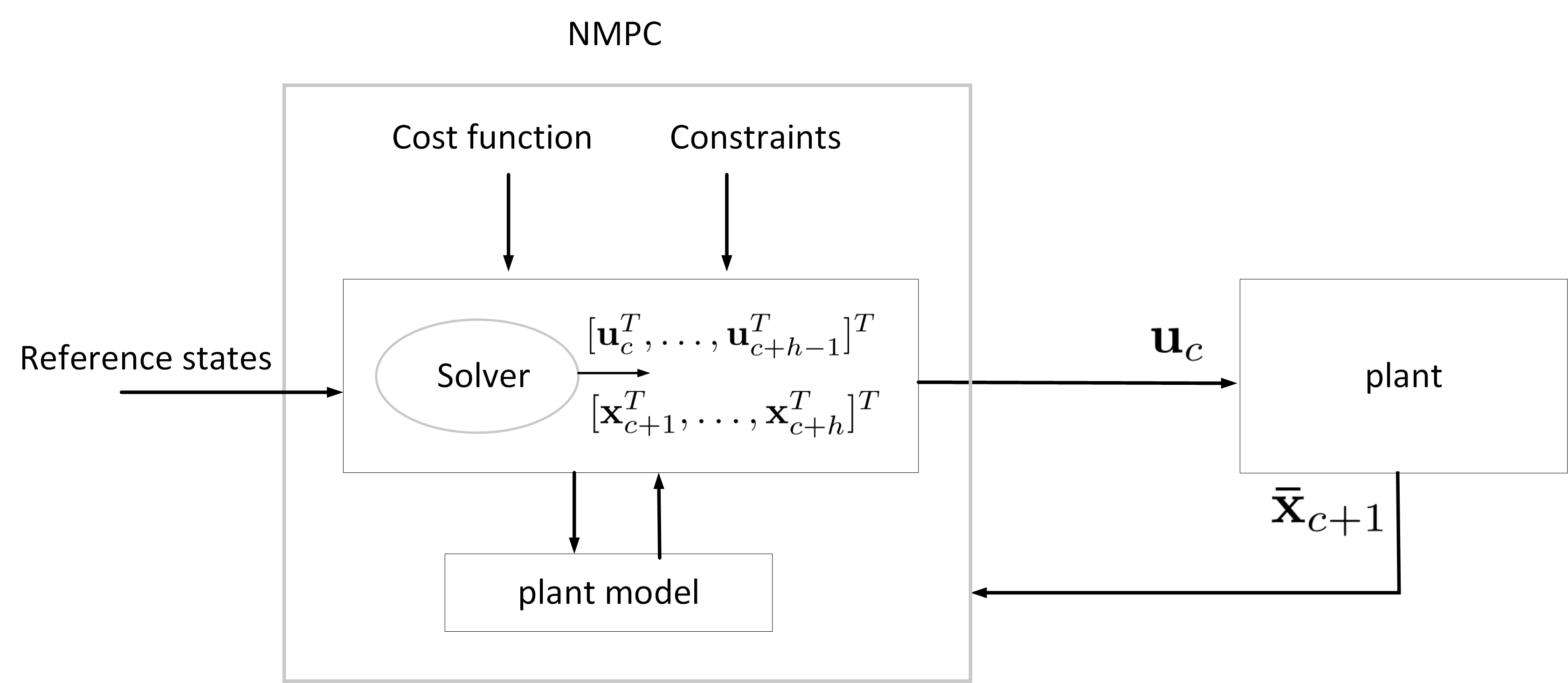
Figure 1: Non-linear model predictive control (NMPC) overall architecture. At each control cycle, NMPC estimates the optimal vector of system inputs $[\mathbf{u}^{T}_{c},\dots,\mathbf{u}^{T}_{c+h-1}]^{T}$ that satisfies a given set of constraints for a fixed horizon length of $h$ time steps. Only the first control input ($\mathbf{u}_{c}$) is applied to the system and new system states ($\mathbf{\bar{x}}_{c+1}$) are produced, and this process is repeated in the next control cycle of NMPC.

III-A1 Unmanned aerial vehicle

We consider here an unmanned aerial vehicle (UAV) that is an aircraft with four rotors [21]. Its motion is controlled by adjusting the angular velocities of these four rotors, i.e., the inputs are a vector of size $n=4$ that contains the angular velocities of the four rotors. The states of the UAV are determined by position, angular velocities, linear velocities, and orientations of the UAV, where each has three values corresponding to the 3D $X$, $Y$, and $Z$ dimensions. Thus, the state vector has size $m=12$ values [21]. The cost function of the UAV’s model is constructed to penalize the error between the current UAV states with respect to their reference position states and penalize the velocities of the four rotors. Specifically, the cost function at time instant $c$ is

$$J(\mathbf{z}_{c})=\sum_{k=c}^{c+h-1}\left(\left[\mathbf{r}_{k+1}-\mathbf{x}_{k+1}\right]^{T}\mathbf{Q}\left[\mathbf{r}_{k+1}-\mathbf{x}_{k+1}\right]\right.\left.+\left[\mathbf{v}_{k}-\mathbf{u}_{k}\right]^{T}\mathbf{R}\left[\mathbf{v}_{k}-\mathbf{u}_{k}\right]\right),$$ (3)

where, $\mathbf{r}_{k}=[r^{1}_{k},\dots,r^{m}_{k}]^{T}$ and $\mathbf{v}_{k}=[v^{1}_{k},\dots,v^{n}_{k}]^{T}$ are the reference states and reference inputs at $k$, respectively. The matrix $\mathbf{Q}=\text{diag}(q^{1},\dots,q^{m})$ weighs the error between the reference and the system states according to the importance of each element of the state vector. The matrix $\mathbf{R}$ weighs the importance of the angular velocities of the four rotors. A box constraint is set to limit the states of the UAV to a certain range. Also, a box constraint is set to limit the velocities of the four rotors into a certain range as

$$\mathcal{U}=\{\mathbf{a}:\mathbf{u}_{\text{min}}\leq\mathbf{a}\leq\mathbf{u}_{\text{max}}\},$$ (4)

$$\mathcal{X}=\{\mathbf{b}:\mathbf{x}_{\text{min}}\leq\mathbf{b}\leq\mathbf{x}_{\text{max}}\},$$

where $\mathbf{u}_{\text{min}}$ and $\mathbf{u_{\text{max}}}$ are the minimum and maximum bounds of the inputs, respectively. $\mathbf{x}_{\text{min}}$ and $\mathbf{x_{\text{max}}}$ are the minimum and maximum bounds of the states, respectively.

The complete UAV model and its parameter settings are presented with more details in Sec. S.I in the supplementary material. The UAV’s model shows a complex system with twelve states and four inputs, with non-linear dynamics. Specifically, the states vary with time, including non-linearities inherited in its model, like trigonometric functions. These factors make the optimization non-convex and challenging to solve using traditional NMPC solvers.

III-A2 Ground vehicle

Here, we consider an autonomous vehicle, where its motion is controlled by adjusting its steering angle and acceleration, i.e., the inputs are a vector of size $n=2$. Longitudinal and lateral positions, longitudinal and lateral linear velocities, yaw angle, and yaw rate determine the states of the vehicle. Thus, the state vector has size $m=6$ values [22]. The cost function of the NMPC for this model is designed to penalize any discrepancies between the vehicle’s longitudinal and lateral positions and orientation and their corresponding references. Moreover, it ensures the smoothness of control input changes by adhering to imposed constraints on both states and inputs [9]. The cost function is formulated as predefined in (3) with a minor modification to account for the safety and comfort of human passengers. Specifically, when the MPC algorithm encounters certain conditions, such as emergency maneuvers or sudden changes in driving conditions, it may be necessary to adjust the weight matrices $\mathbf{Q}$ and $\mathbf{R}$ in the cost function (3) to achieve the desired performance. Let us define $cond1$ to be true whenever any of these conditions occur, then the $\mathbf{Q}$ and $\mathbf{R}$ matrices are adjusted as

$$\mathbf{Q}=\begin{cases}\mathbf{Q}_{1}&\text{if }cond1,\\ \mathbf{Q}_{0}&\text{otherwise},\end{cases}$$ (5)

$$\mathbf{R}=\begin{cases}\mathbf{R}_{1}&\text{if }cond1,\\ \mathbf{R}_{0}&\text{otherwise}.\end{cases}$$

Thus, based on $cond1$, the NMPC adjusts $\mathbf{Q}$ by selecting between $\mathbf{Q}_{0}$ and $\mathbf{Q}_{1}$, where each matrix differently weighs the error between the reference and the system states according to the importance of each element of the state vector. Similarly, $\mathbf{R}$ is adjusted. The exact values of these matrices and more information regarding this vehicle model and its parameter settings are presented in the supplementary material in Sec. S.II.

In order to confine the vehicle states and inputs within predetermined boundaries, box constraints are implemented. A box constraint is applied to limit the vehicle states within specific bounds, and another is applied to restrict the acceleration and steering angle inputs to defined boundaries, as predefined in (4). As shown in Sec. S.II, the model indicates the presence of nonlinearities, and the cost function has variable weights and discontinuities. Solving such complex and discontinuous optimization problem is challenging, even using nonlinear solvers. The subsequent section presents the genetic algorithm, demonstrating the potential to solve such complex optimization problem.

III-B Genetic algorithm as a nonlinear model predictive control solver

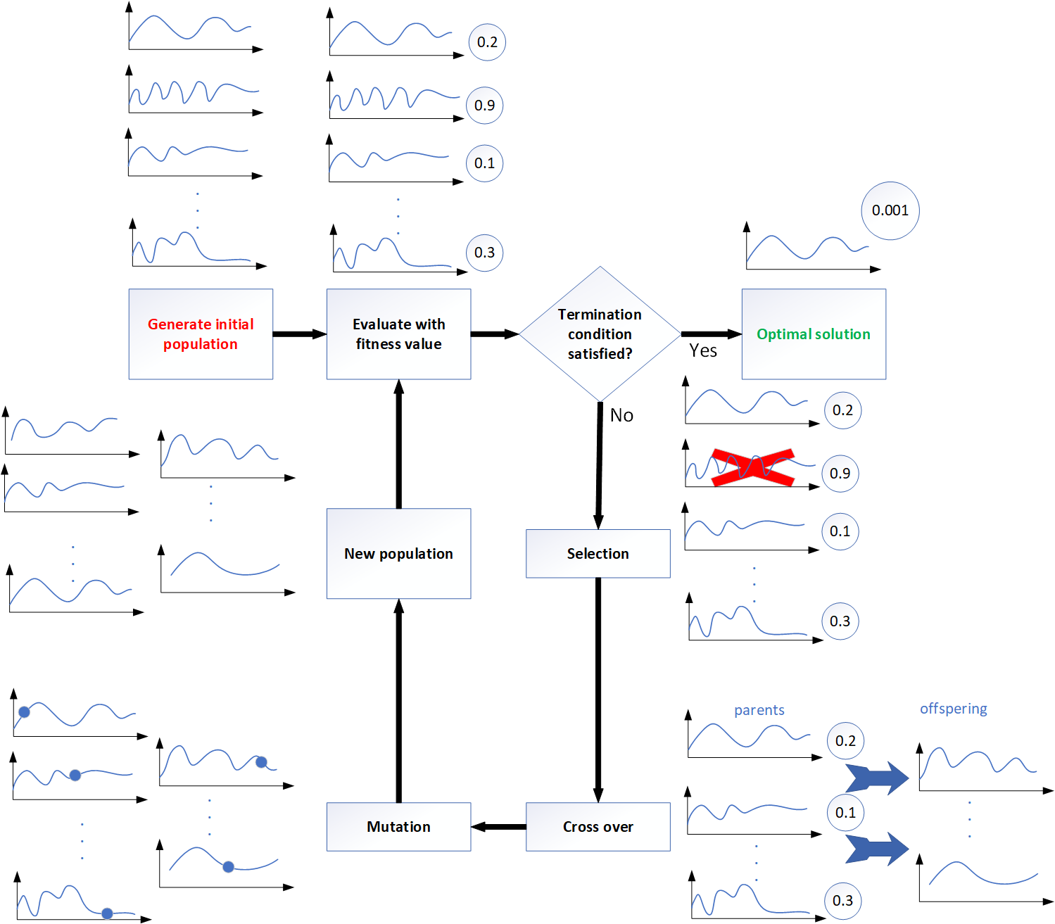
Figure 2: Block diagram of genetic algorithm GA. The GA starts by initializing a population of candidate solutions for the NMPC optimization problem. Then, these solutions are evaluated, and the best solutions are selected based on a selection rule. In each iteration, the selected solutions undergo crossover and mutation to generate a new generation of solutions. This iterative process continues until a termination condition is met or convergence occurs.

The GA is exceptional in solving several complicated NMPC optimization problems compared with other classical optimization solvers techniques, especially when the optimization problem involves non-linearities or if/else conditions. This merit comes from the fact that the GA does not include any differential calculations or gradient evaluations. Specifically, the GA uses evolutionary information to direct the search within the solution search space to obtain the optimal solution that satisfies the control problem constraints. A general GA architecture is illustrated in Fig. 2. The GA starts with a population of solutions (chromosomes) representing candidates’ solutions of the NMPC optimization problem. Each solution $\mathbf{z}_{c}$ is composed of $hn$ values named genes. The solutions evolved through successive iterations, called generations. At each iteration, a new generation of offspring solutions is produced from the parent solutions using the crossover and mutation processes. The crossover process merges two or more solutions to generate new ones, while the mutation is a random modification of randomly selected one or more genes by new random values. Particular crossover and mutation rates govern the probability of applying the modifications. After each generation, all solutions are arranged according to their fitness value [23] such that solutions with the best fitness values have more chances to be selected and be survivable in the next generations. In NMPC, the fitness $F$ of an individual is defined based on the cost function $J$, that is used in the optimization function (2), as

$$F=\frac{1}{(1+J)}.$$ (6)

Based on this fitness value, different selection techniques such as roulette wheel selection, tournament selection, and steady-state selection [24] can be applied. The iterative process is stopped when a termination condition occurs. The termination occurs in two cases. The first is when the solution’s cost falls below a threshold, and the algorithms converge to the optimal solution in this case. Alternatively, when the time elapsed reaches the control cycle time, the algorithm returns a sub-optimal solution.

Since the GA is an evolutionary numerical algorithm that tries several candidate optimal control inputs, exploring the search space by the GA may take a significant amount of time, especially when the solution space is large. This makes the GA not suitable for many applications that require fast response. In the next section, we introduce our proposed approach that accelerates the GA by adaptively changing the size of the search space explored by the GA so that it can reach the optimal solution with a reduced amount of time.

IV Motivation and proposed learning of optimal search space size for genetic optimization

At each control cycle, the GA explores the search space to estimate the control inputs that represent the optimal solution of the optimization problem of the NMPC. The GA uses the notion of margin to represent the search space size. The margin is a constrained solution space region that, with high probability, contains the optimal control inputs. The margin setting is crucial for obtaining good performance with a fair amount of computations. A small margin lowers the probability of finding the optimal inputs in the current cycle. In contrast, a large margin increases this probability by the expenses of more computations.

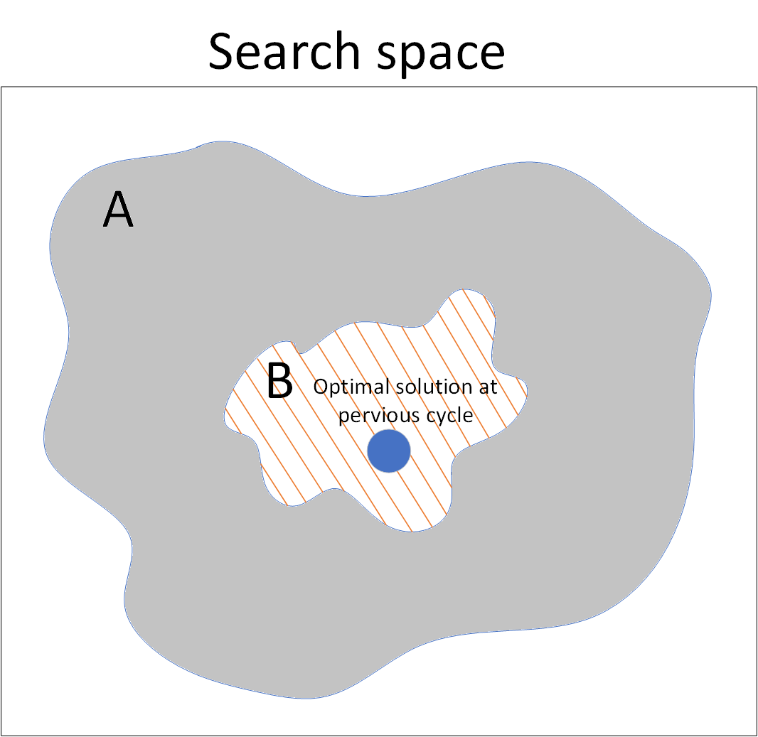
(a)

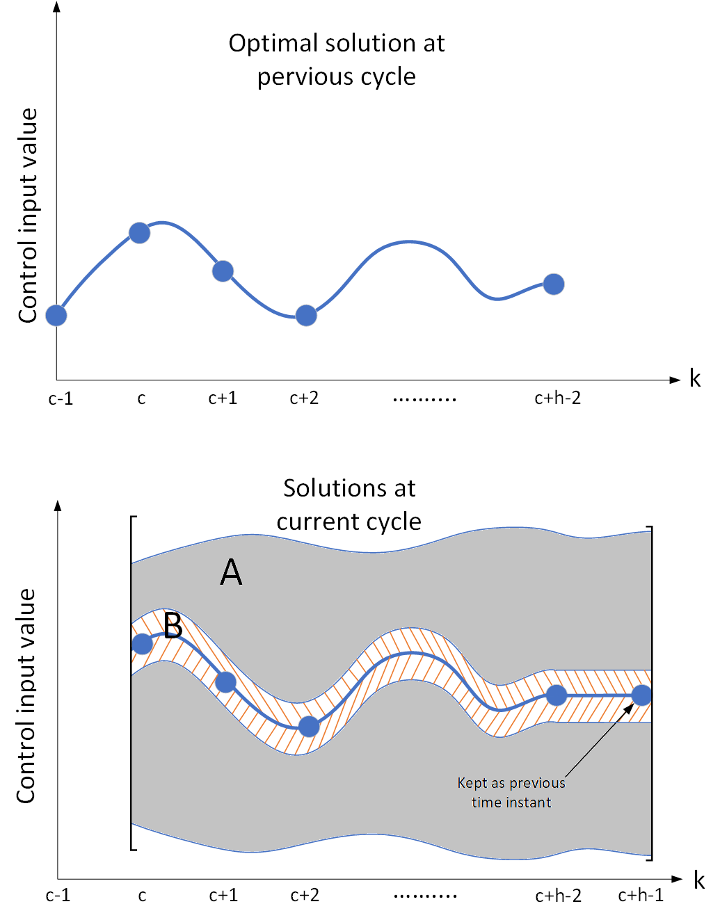
(b)

Figure 3: A Graphical representation of the search spaces of GA. In (a), we show a contour (A) that represents the search space that comes from the physical constraints of the system, and another contour (B) marked with dashed red lines represents the BSM. In (b), we show how the candidate control inputs solutions at the current cycle are obtained by time-shifting the previous cycle control inputs by one time step and searching around it in the BSM region marked by dashed red lines.

One way to set this margin is to match it with the system’s physical constraints (physical margin) because no optimal control inputs can be found outside this margin, i.e., do not satisfy the system’s constraints. This can be represented by the area labeled (A) in Fig. 3. However, the physical constraints may have large bounds, which still makes the search space large. Another way is to set the margin at a current control cycle to be a specific neighborhood around the optimal control inputs that are estimated at the previous cycle shifted by one time step, as the area labeled (B) in the figure. As the figure shows, the optimal control inputs in the $c^{\text{th}}$ control cycle fall at a neighborhood around the optimal control inputs at the $(c-1)^{\text{th}}$ control cycle shifted by one time step. However, because the GA is an evolutionary algorithm, it may not converge to the optimal control inputs in the previous cycle. Thus, the setting of this margin is prone to an accumulation of errors in the control inputs with the progression of the cycles. To avoid this, a restriction can be made to set this margin only around the previous control inputs if the solution is optimal, i.e., its cost falls below a threshold. Otherwise, the physical constraints will be used as the margin. This margin setting dramatically reduces the search space compared with the system’s physical constraints and simultaneously avoids any accumulation of errors in the control inputs with the progression of the cycles.

In this paper, we are interested in finding the best smallest margin (BSM), i.e., the smallest margin where the optimal control inputs lie around the previously founded optimal control inputs. Finding such a margin will significantly improve the chance of obtaining the optimal control inputs in the current cycle within the shortest computational time. Throughout the rest of the paper, we denote the BSM of the $c^{\text{th}}$ control cycle as $\boldsymbol{\Delta}_{c}$ as we define next.

Definition 1: Best smallest margin $\boldsymbol{\Delta}_{c}$

• Let $\mathbf{g}^{i}_{c}=[u^{i}_{c},\dots,u^{i}_{c+h-1}]$ be a vector that contains the values of the $i^{\text{th}}$ control input along the horizon $h$ in the $c^{\textnormal{th}}$ control cycle. As depicted in Fig. 4, we define $\delta_{c}^{i}$ as the maximum of absolute differences between the corresponding elements of $\mathbf{g}^{i}_{c}$ that is estimated at the current $c^{\text{th}}$ and previous $c^{\text{th-1}}$ control cycles. Then, the BSM vector is defined as

  $$\boldsymbol{\Delta}_{c}=\begin{cases}[\delta_{c}^{1},\dots,\delta_{c}^{n}]&\text{if }J(\mathbf{z}^{*}_{c-1})\leq\epsilon,\\ [\beta^{1},\dots,\beta^{n}]&\text{otherwise,}\end{cases}$$ (7)

  where $\beta^{i}$ is the physical margin of the $i^{\text{th}}$ control input and $\epsilon$ is a threshold that determines whether the solution at the previous cycle is optimal. The setting of $\epsilon$ is application dependent and according to the required level of optimality.

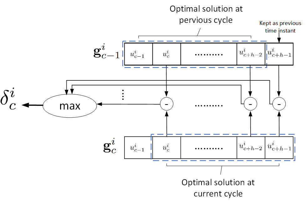
Figure 4: Graphical illustration that presents the definition of $\delta_{c}^{i}$. We define $\delta_{c}^{i}$ as the maximum of absolute differences between the corresponding elements of $\mathbf{g}^{i}_{c}$ that is estimated at the current $c^{\text{th}}$ and previous $c^{\text{th-1}}$ control cycles.

In the following, we present the proposed approach that adaptively estimates the BSM. First, we motivate the proposed approach from the point of view of the main factor that affects the BSM. Then, we present the proposed approach in detail.

IV-A Motivation

In NMPC, the optimal control inputs are estimated in each control cycle for a future horizon $h$. However, instead of time-shifting these readily computed optimal control inputs in the next cycle, the NMPC estimates new optimal control inputs. This is mainly because the system’s future behavior may deviate from the expected behavior due to various factors such as disturbances, model uncertainties, or changes in the system dynamics. Therefore, the NMPC continuously estimates the optimal control inputs to cope with the changing conditions of the system and ensures that the optimal control action is taken at each control cycle, instead of depending on time-shifted previously estimated inputs.

Intuitively, suppose there are low disturbances and/or small changes in system state dynamics. In that case, the expected current system states $\mathbf{x}_{c}$ that is obtained by applying the optimal control inputs estimated from the previous cycle in the mathematical model of the system (1), will slightly differ from the measured states in the current cycle $\mathbf{\bar{x}}_{c}$. Thus, we expect that the optimal control inputs at the current cycle differ slightly from the previously estimated (time-shifted) inputs in the previous cycle. This means that the values of the BSM will be small in this case. In contrast, if there is a considerable disturbance and/or abrupt change in system state dynamics, $\mathbf{x}_{c}$ will have big differences from $\mathbf{\bar{x}}_{c}$. This means that the system needs to make an aggressive change in the control inputs from the previously estimated control inputs in the previous cycle. Therefore larger values for the BSM are required.

To validate the above claim, we perform the following experiment. We use the UAV model discussed in Sec. III-A1 and synthetically add errors that represent random disturbances and abrupt changing in the model states in each control cycle. We estimate the optimal control inputs in each cycle using the GA but with a large margin equal to the UAV model’s physical constraints. Additionally, to neutralize the effect of the initial conditions, we started our experiments with initial state values equal to initial reference state values. In each cycle, we obtain the associated BSM (as defined in Definition 1) and record its maximum $\Delta_{c}^{\max}=\max(\boldsymbol{\Delta}_{c})$. Also, we quantify the difference between $\mathbf{x}_{c}$ and $\mathbf{\bar{x}}_{c}$ by $\mathbf{\mathcal{E}}_{c}$ defined as

$$\mathbf{\mathcal{E}}_{c}=[q^{1}(\bar{x}^{1}_{c}-x^{1}_{c})^{2},\dots,q^{m}(\bar{x}^{m}_{c}-x^{m}_{c})^{2}],$$ (8)

and record its maximum $\mathcal{E}_{c}^{\max}=\max(\mathbf{\mathcal{E}}_{c})$. We record the maximum values because any disturbance to any system state leads to a corresponding change in one or more control inputs because of the coupling between the inputs.

We ran the experiment several times and gathered the recorded $\mathcal{E}_{c}^{\max}$ and $\Delta_{c}^{\max}$ in all cycles. We sort the gathered values of $\mathcal{E}_{c}^{\max}$ in 10 percentiles and plot the corresponding $\Delta_{c}^{\max}$ against $\mathcal{E}_{c}^{\max}$ using the box plots in Fig. 5. As shown in the figure, $\Delta_{c}^{\max}$ increases with the increase in $\mathcal{E}_{c}^{\max}$. Consequently, we can conclude that the $\Delta_{c}^{\max}$ of a control cycle is proportionally related to the error between the expected and measured system states in the control cycle.

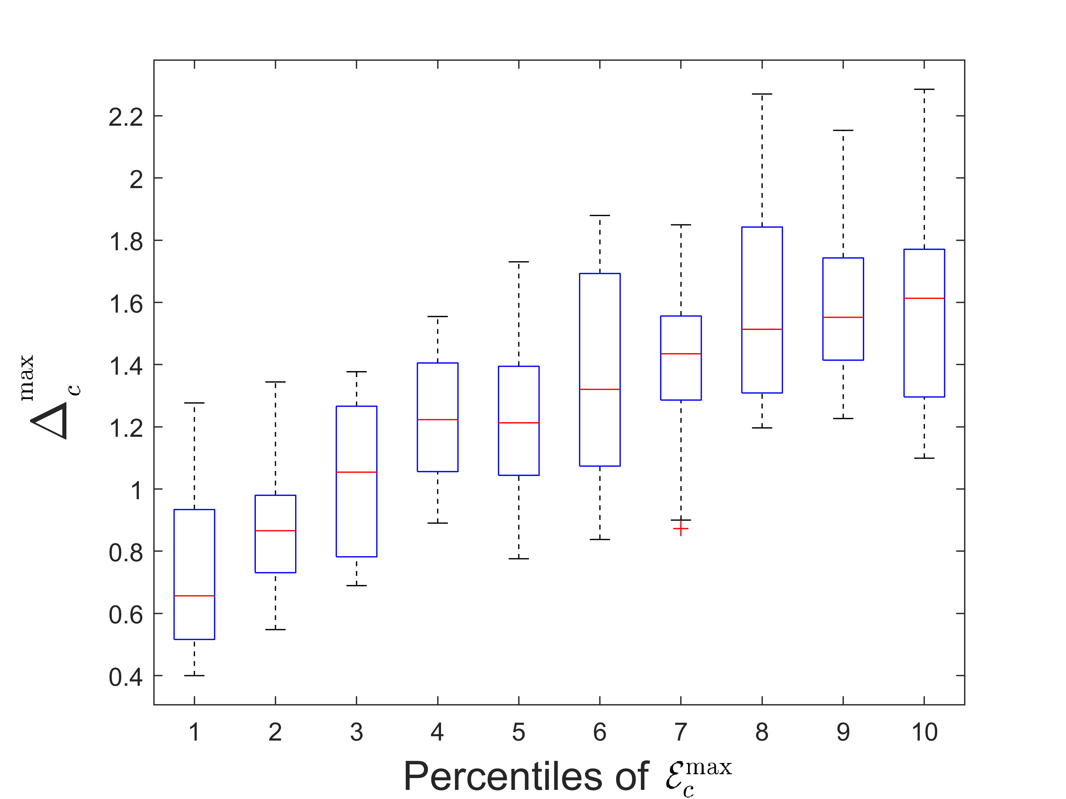
Figure 5: A box plot shows the relation between the values of $\{\mathcal{E}_{c}^{\max}\}$ sorted in 10 percentiles and their corresponding $\Delta_{c}^{\max}$ values. The $\Delta_{c}^{\max}$ increases as $\mathcal{E}_{c}^{\max}$ increases.

We ran the experiment several times and gathered the recorded $\mathcal{E}_{c}^{\max}$ and $\Delta_{c}^{\max}$ in all cycles. We sort the gathered values of $\mathcal{E}_{c}^{\max}$ in 10 percentiles and plot the corresponding $\Delta_{c}^{\max}$ against $\mathcal{E}_{c}^{\max}$ using the box plots in Fig. 5. As shown in the figure, $\Delta_{c}^{\max}$ increases with the increase in $\mathcal{E}_{c}^{\max}$. Consequently, we can conclude that the $\Delta_{c}^{\max}$ of a control cycle is proportionally related to the error between the expected and measured system states in the control cycle.

From the outcomes of the above experiment, one can estimate a mathematical relation that relates $\mathcal{E}_{c}^{\max}$ with $\Delta_{c}^{\max}$ and use this relation in the GA optimization to find the BSM to limit the search space at each cycle adaptively. However, the experiment is just for illustration and is far from realistic scenarios. This is because we used the maximum value among the elements of the BSM vector to report the results to neutralize the coupling effect between the control inputs. However, in real scenarios, we need to estimate the whole $\boldsymbol{\Delta}_{c}$ vector in which each element is the corresponding control input’s margin, as stated in Definition 1.

In the next section, we present our proposed approach, which predicts $\boldsymbol{\Delta}_{c}$ according to error vector extracted in each cycle using a multivariate non-linear support vector regression algorithm.

IV-B Proposed learning of optimal search space size for genetic optimization

This section presents our proposed approach that estimates the optimal search space size for genetic optimization of NMPC by estimating the best smallest margin $\boldsymbol{\Delta}_{c}$. The proposed approach uses $n$ regression models to adaptively predict $\delta_{c}^{i}$ for each control input in every control cycle. To build the regression models, we first build a synthetic dataset using the model of the system we want to control. Then, we train the regression models on the dataset. In runtime, we use the trained regression models to estimate $\delta_{c}^{i}$ for each control input and form the best smallest margin $\boldsymbol{\Delta}_{c}$ from Eq. 7.

We use simulation techniques to build the dataset by randomly varying the system’s control inputs while satisfying its constraints. This allows us to generate numerous $N$ cycles of reference states. As in Sec. IV-A, we synthetically add errors representing random disturbances and abrupt changes in the model states in each control cycle. Moreover, the control inputs are estimated in each cycle using the GA but with a large margin equal to the physical constraints of the system. Additionally, we use a large population size and a large number of generations with no termination condition, meaning that the GA continues its calculations until it reaches the end of its generations. This ensures we converge to the optimal solution with high probability so $\delta_{c}^{i}$ for each input is correctly estimated. Thus, each record in the dataset contains the error vector $\mathbf{\mathcal{E}}_{c}$ of the $c^{\text{th}}$ control cycle and its associated $n$ values of $\delta_{c}^{i}$.

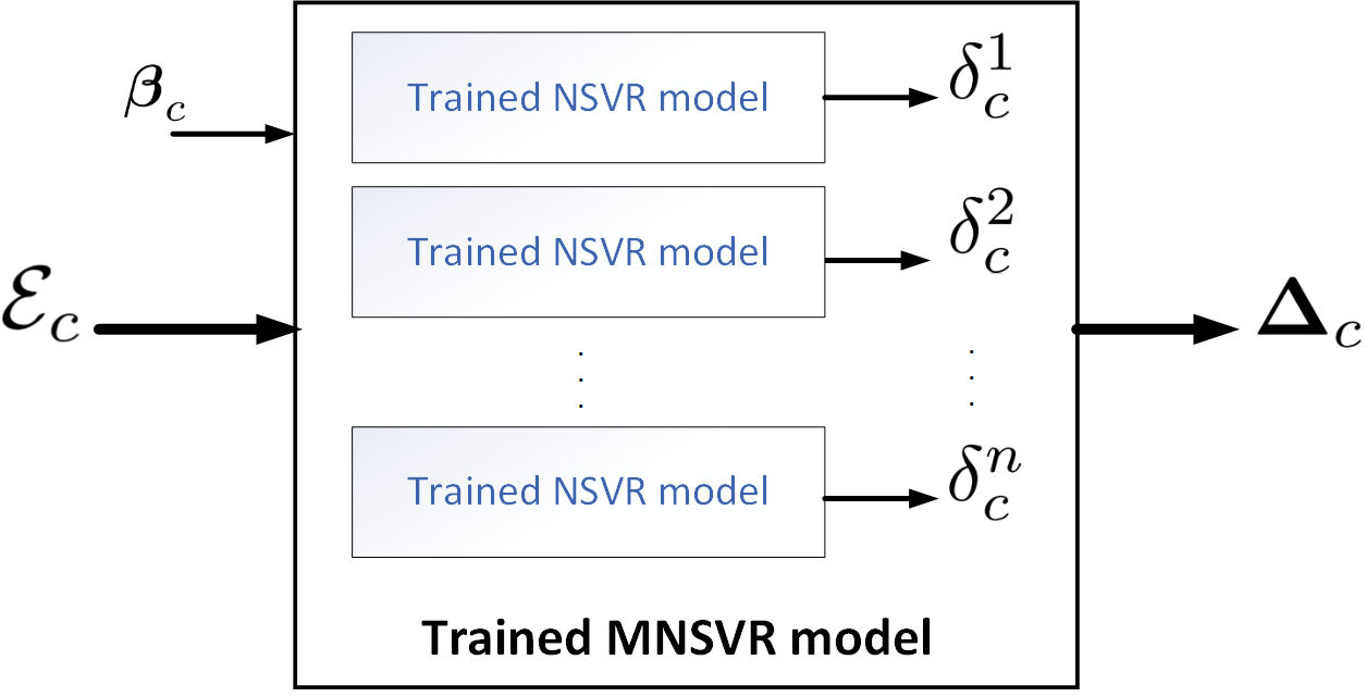
Figure 6: Block diagram of the estimation of $\boldsymbol{\Delta}_{c}$ in run time using the trained multivariate nonlinear support vector regressors (MNSVR).

We use a multivariate nonlinear support vector regressor (MNSVR) [25] for building our regression models. Specifically, our MNSVR contains $n$ nonlinear support vector regressors, one for predicting each $\delta_{c}^{i}$. Each regressor estimates the relationship between the error vector $\mathbf{\mathcal{E}}_{c}$ and $\delta_{c}^{i}$. Specifically, the $i^{\text{th}}$ regressor finds the hyperplane $\mathbf{{\boldsymbol{\omega}}}_{i}^{T}\phi(\mathbf{\mathcal{E}}_{c})+b_{i}$ that fits the maximum number of all $\delta_{c}^{i}$ in the dataset within a margin $\lambda$ from the hyperplane, where $\phi(\mathbf{\mathcal{E}}_{c})$ is a nonlinear transformation that maps $\mathbf{\mathcal{E}}_{c}$ to a higher-dimensional space. The goal of the training is to find the best parameters $\{{\boldsymbol{\omega}}^{*}_{i},b^{*}_{i}\}$, $\forall i=1,\dots,n$, for the MNSVR.

In the runtime, as depicted in Fig. 6, each regression model receives the input vector $\mathbf{\mathcal{E}}_{c}$ for each control cycle and estimates

$$\delta_{c}^{i}={\boldsymbol{\omega}}^{*T}_{i}\phi(\mathbf{\mathcal{E}}_{c})+b^{*}_{i},\;\forall i=1,\dots,n,$$ (9)

and the best smallest margin $\boldsymbol{\Delta}_{c}$ is formed according to Eq. 7. To generate a population of candidate solutions for the GA, we sample $p_{c}$ solutions randomly within $\boldsymbol{\Delta}_{c}$. In order to make $p_{c}$ to be not dependent on the scale of a specific control input, we normalize $\boldsymbol{\Delta}_{c}$ according to the physical margin of each input. Specifically, we compute the normalized margin $\bar{\delta_{c}}^{i}$ for the $i^{\text{th}}$ control input as $\bar{\delta_{c}}^{i}=\delta_{c}^{i}/\beta^{i}$. Then, we compute the maximum of all normalized margins as $\alpha_{c}=\max\{\bar{\delta_{c}}^{i}\}$, where $i=1,\dots,n$. Finally, we set $p_{c}$ as

$$p_{c}=\max\{\lfloor\sigma\alpha_{c}\rfloor,\gamma\},$$ (10)

where $\sigma$ represents the sampling density and $\gamma$ represents a minimum population size that ensures we generate enough candidate solutions even within small estimated margins. Once a population of $p_{c}$ candidate solutions is generated, GA proceeds normally to determine the optimal solution, as discussed in Sec. III-B. The complete process of the proposed approach is illustrated in Algorithm 1.

Algorithm 1 Proposed learning of optimal search space size for genetic optimization.

1:$N$: is the number of generated reference states for training the MNSVR.

2:$H$: is the number of control cycles.

3:$G$: is the number of generations.

4:Generate $N$ cycles of reference states.

5:$c$ $\leftarrow$ 0.

6:while $c<N$ do

7:     Compute $\mathbf{\mathcal{E}}_{c}$ using (8), and its associated $n$ values of $\delta_{c}^{i}$.

8:     Add $\mathbf{\mathcal{E}}_{c}$ along with its associated $n$ values of $\delta_{c}^{i}$ to the dataset records.

9:     $c\leftarrow c+1$.

10:end while

11:Train $n$ MNSVR models to estimate $\{{\boldsymbol{\omega}}^{*}_{i},b^{*}_{i}\}$, $\forall i=1,\dots,n$.

12:$c$ $\leftarrow$ 0.

13:while $c<H$ do

14:     Compute $\mathbf{\mathcal{E}}_{c}$ using (8).

15:     $\delta_{c}^{i}$ $\leftarrow$ ${\boldsymbol{\omega}}^{*T}_{i}\phi(\mathbf{\mathcal{E}}_{c})+b^{*}_{i}$, $\forall i=1,\dots,n$.

16:     Compute $\boldsymbol{\Delta}_{c}$ using (7).

17:     Compute $p_{c}$ using (10).

18:     Generate $p_{c}$ solutions around the previous inputs.

19:     $g\leftarrow 0$.

20:     while $g<G$ do

21:         Calculate solutions fitness using (6).

22:         Sort solutions according to their fitness values.

23:         $\mathbf{z}_{c}^{*}\leftarrow$ solution with the minimum fitness.

24:         if $J(\mathbf{z}_{c}^{*})\leq\epsilon$ then

25:              break.

26:         end if

27:         Apply selection, cross over and mutation operations.

28:         $g\leftarrow g+1$.

29:     end while

30:     Get the first $n$ elements from $\mathbf{z}_{c}^{*}$ as the optimal input $\mathbf{u}_{c}\leftarrow\mathbf{z}_{c}^{*}[1:n]$.

31:     Apply the optimal input $\mathbf{u}_{c}$ to the plant and get the new states $\mathbf{\bar{x}}_{c+1}$.

32:     $c\leftarrow c+1$.

33:end while

IV-C GA implementation on a GPU

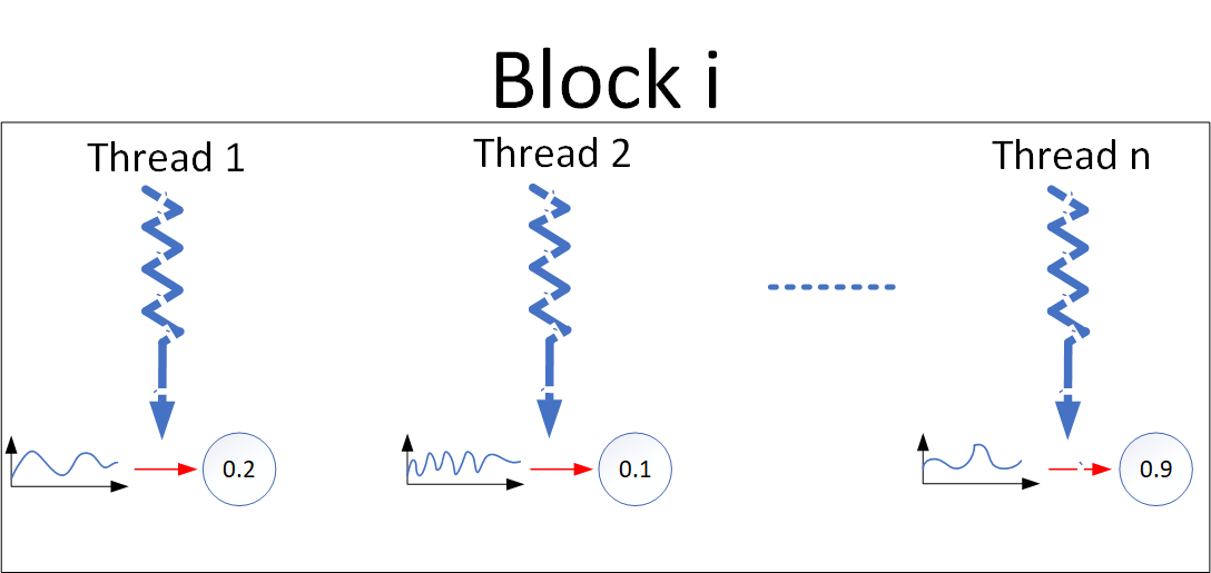
(a) Fitness calculations

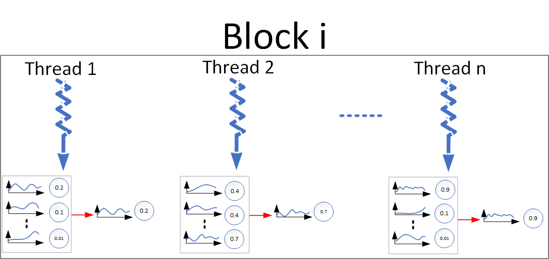
(b) Selection

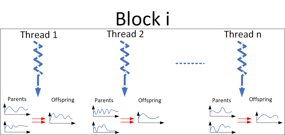
(c) Cross over

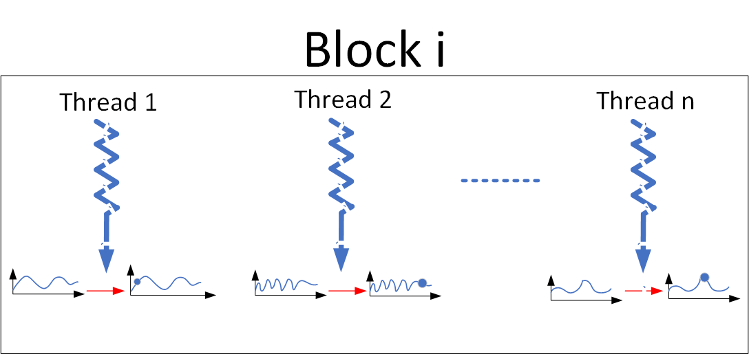
(d) Mutation

Figure 7: Graphical representation of the CUDA programming model of the implementation of GA on GPU. We harness the capabilities of the GPU by parallelizing the calculations of GA that includes (a) the concurrent evaluation of the fitness function of multiple solutions, (b) the selection, (c) the crossover, and (d) the mutation operations.

GPUs are designed to enable the parallel processing of numerous threads, each executing identical operations on different data. These threads are assigned unique indices by the CUDA programming interface and are organized into blocks. Threads within a block may execute synchronously and share a common memory. Our implementation leverages the capabilities of the GPU of Nvidia Jetson TX2, which features a hex-core ARMv8 64-bit CPU complex, 8GB LPDDR4 memory, an integrated 256-core NVIDIA Pascal GPU, and a 128-bit interface. We break down the genetic computation involved in solving NMPC optimization into smaller parallel tasks to be suitable for the GPU. Running these tasks concurrently across multiple threads can lead to significant performance improvements compared to implementing GA on CPU-based programming. We harness the capabilities of the GPU of the Jetson TX2 platform for parallel computing in the following ways.

1. The concurrent evaluation of the fitness function of multiple solutions, as shown in Fig. 7 (a). This is obtained by assigning a thread to each solution to compute its fitness.

2. We parallelize the GA operators, including selection, mutation, and crossover, as presented below.

   • Selection is parallelized by dividing the population into subsets as shown in Fig. 7 (b), with each subset assigned to a thread. Each thread then selects the fittest individuals in its assigned subset, returning the selected individuals to be used in the next generation of the population.

   • Crossover is parallelized by dividing the population into pairs of parents, with each pair assigned to a thread. Each thread then performs the operation of crossover on the two parents to generate the new offspring, as seen in Fig. 7 (c), resulting in multiple offspring being generated concurrently.

   • Mutation is parallelized by modifying the solutions in parallel. Each thread is assigned to modify a particular solution in the population. Thus, the modification process is applied to multiple solutions simultaneously, as shown in Fig. 7 (d).

3. Sorting of the solutions based on their fitness values is parallelized using a parallel merge sort algorithm. Specifically, this algorithm operates by breaking down the fitness values of solutions into smaller subarrays, sorting them independently in parallel, and then merging the sorted subarrays to obtain the final sorted result.

V Experimental results

In this section, we experimentally evaluate and compare the proposed adaptive approach that adaptively changes the genetic optimization search space size and compares its performance with two approaches: the traditional genetic approach that uses fixed search space and the modified version of the traditional genetic algorithm proposed in [8, 9]. We denote the proposed adaptive approach as AG and the other approaches under comparison as FG and MFG, respectively. All of this approaches are compared when controlling the nonlinear UAV and vehicle models, discussed in Sec. III-A1 and III-A2, respectively, with NMPC. We assume that the states of both models are measurable to the NMPC. To train the regression models for AG, we create a dataset containing N = 10,000,000 records for each of the UAV and vehicle models. The parameters of the regression models are estimated using the 5-fold cross-validation technique [26], and presented in Sec. S.III in the supplementary material.

Our comparison is performed regarding both the performance and the computational time. We evaluate the performance metric as the average cost over all control cycles. Assume that we have $H$ control cycles, the average cost $E$ is computed as

$$E=\frac{1}{H}\sum_{c=1}^{H}J(\mathbf{z}_{c}^{*}).$$ (11)

All approaches are implemented on the GPU of a Nvidia^™ Jetson TX2 embedded platform in a processor-in-the-loop (PIL) fashion. In all experiments, the settings of both approaches are kept the same for a fair comparison.

In the following, we first present the PIL setup. Then, we present our experiments to compare AG with the other approaches.

V-A Processor-in-the-loop setup

As illustrated in Fig. 8, our hardware-in-the-loop setup consists of two components: a plant simulator running on a host machine and the NMPC controller running on an embedded target. These two components are connected via an RS232 Ethernet cable. The host machine sends reference inputs and states to the controller and measures the plant dynamics after applying the control inputs. The host machine is a laptop running Microsoft Windows 10 OS with an Intel-i7 8700 CPU and 16 GB of RAM. The implementation of both the nonlinear UAV and vehicle planet models on the host machine is written in MATLAB. The embedded target is an NVIDIA Jetson TX2, running Ubuntu 16.04.

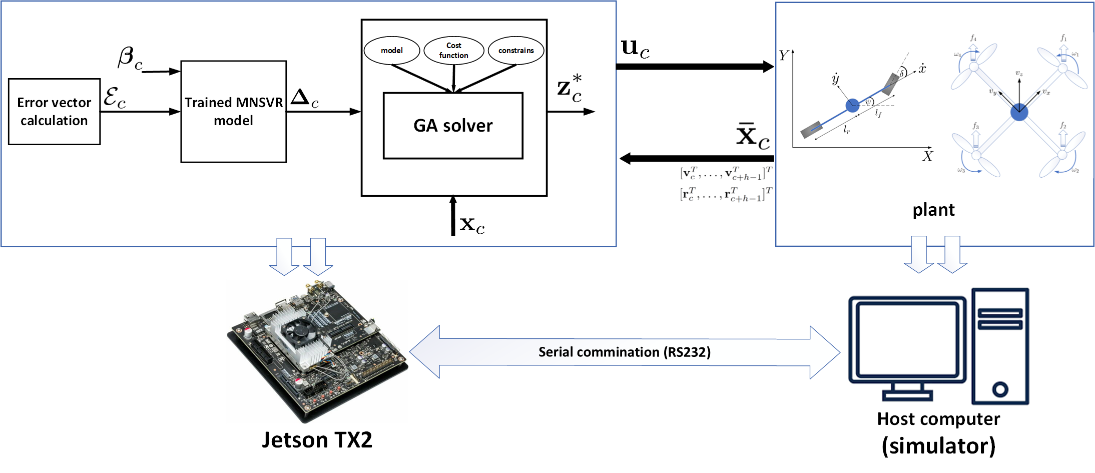
Figure 8: The processor-in-the-loop setup.

For the UAV model, we are interested in controlling the UAV motion in the 3D space. The UAV’s plant simulator takes the rotors’ velocities from the controller as control inputs and outputs the position, angular velocities, linear velocities, and orientations of the UAV. For the ground vehicle, we are interested in controlling the vehicle’s longitudinal and lateral positions and orientation. The vehicle’s plant simulator takes the steering angle and acceleration from the controller as control inputs. It outputs the longitudinal and lateral positions, longitudinal and lateral linear velocities, yaw angle, and yaw rate. The reference states used in our experiments are designed to contain both rabid and slow variations to reflect real-world scenarios and make the simulation more realistic. The reference states for UAV and Vehicle are shown in Fig. S.3 in the supplementary material. The optimization parameter settings utilized for both the UAV and the ground vehicle are presented in Table S.III and Table S.IV, respectively, in the supplementary material.

V-B Comparison with other approaches

This section presents our experimental comparison between the proposed adaptive approach (AG) with both the traditional genetic approach (FG) and its modified version (MFG) [9, 8]. As mentioned, the AG approach adjusts the population size $p_{c}$ based on $\boldsymbol{\Delta}_{c}$ in each control cycle using (10), whereas the FG and MFG approaches keep a constant population size across all control cycles. The MFG keeps a constant population size as FG, but its population comprises two parts with different proportions. The first is generated within the fixed physical margin, the same as the FG approach. The other part is set to be a time-shifted version of the best solutions in the last generation of genetic optimization in the previous control cycle.

For a fair comparison, we set the sampling density $\sigma$ in (10) to the same value for all approaches. For FG and MFG approaches, we set the margin to be the physical margin of each control input, i.e., we set $\delta_{c}^{i}=\beta^{i}$ for $i=1,\dots,n$. This means that $\alpha_{c}$ in (10) has the value 1 for FG and MFG approaches. For MFG, 80% of the population is randomly generated within the physical margin, and the remaining 20% is obtained by shifting the best solutions from the previous control cycle one backward time step. We compute the average cost $E$ and the average computational time for all approaches when applying to control the UAV and the vehicle models using the NMPC. Additionally, we compute the percentage of the cycles that each approach converges to the optimal solution before the termination of the cycle’s time. We plot the average computational time, the convergence percentage, and $E$ in Fig. 9 (a), (b), and (c), respectively. The upper row shows the plot for the UAV model, while the bottom one is for the vehicle model.

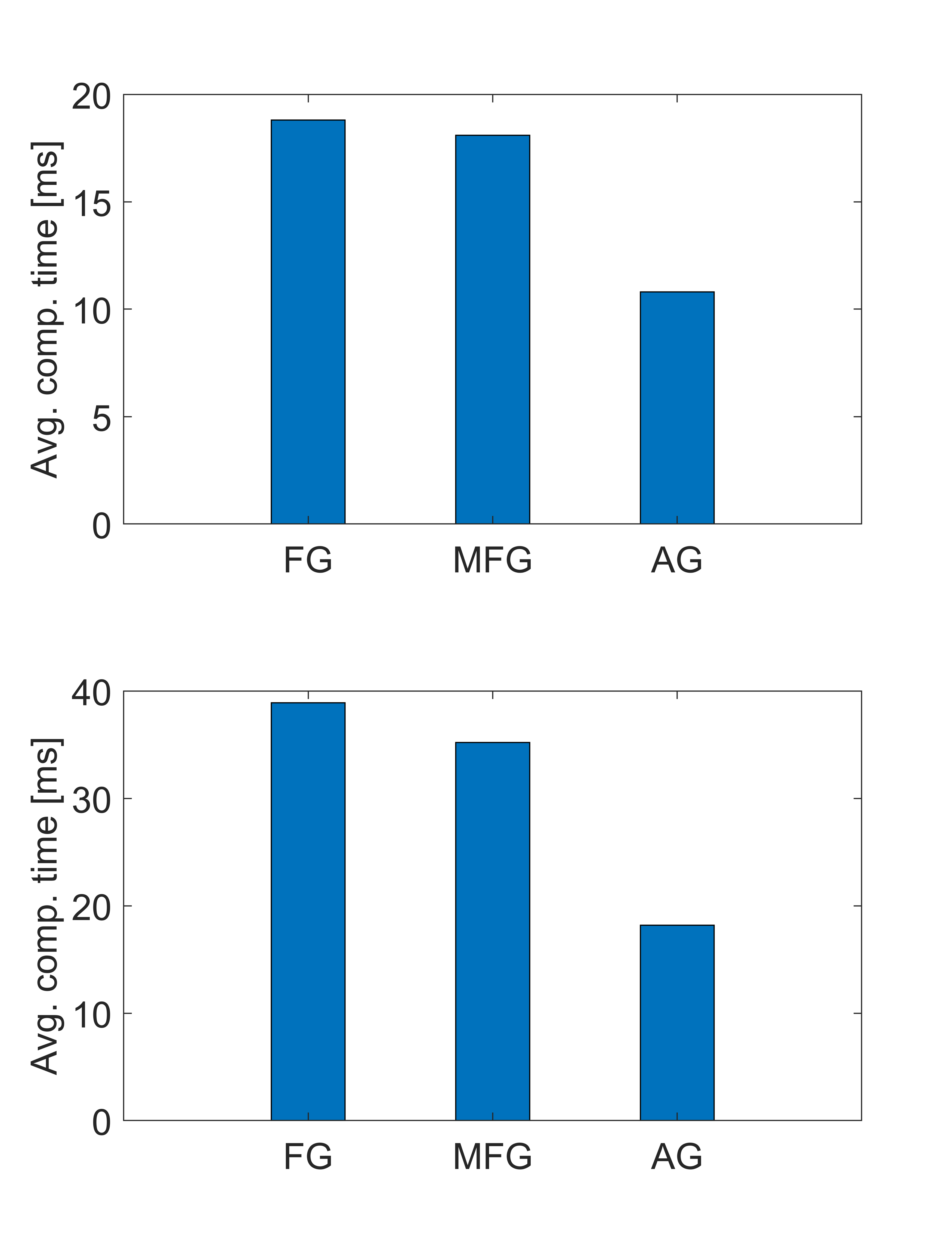
(a) Comp. time $\downarrow$

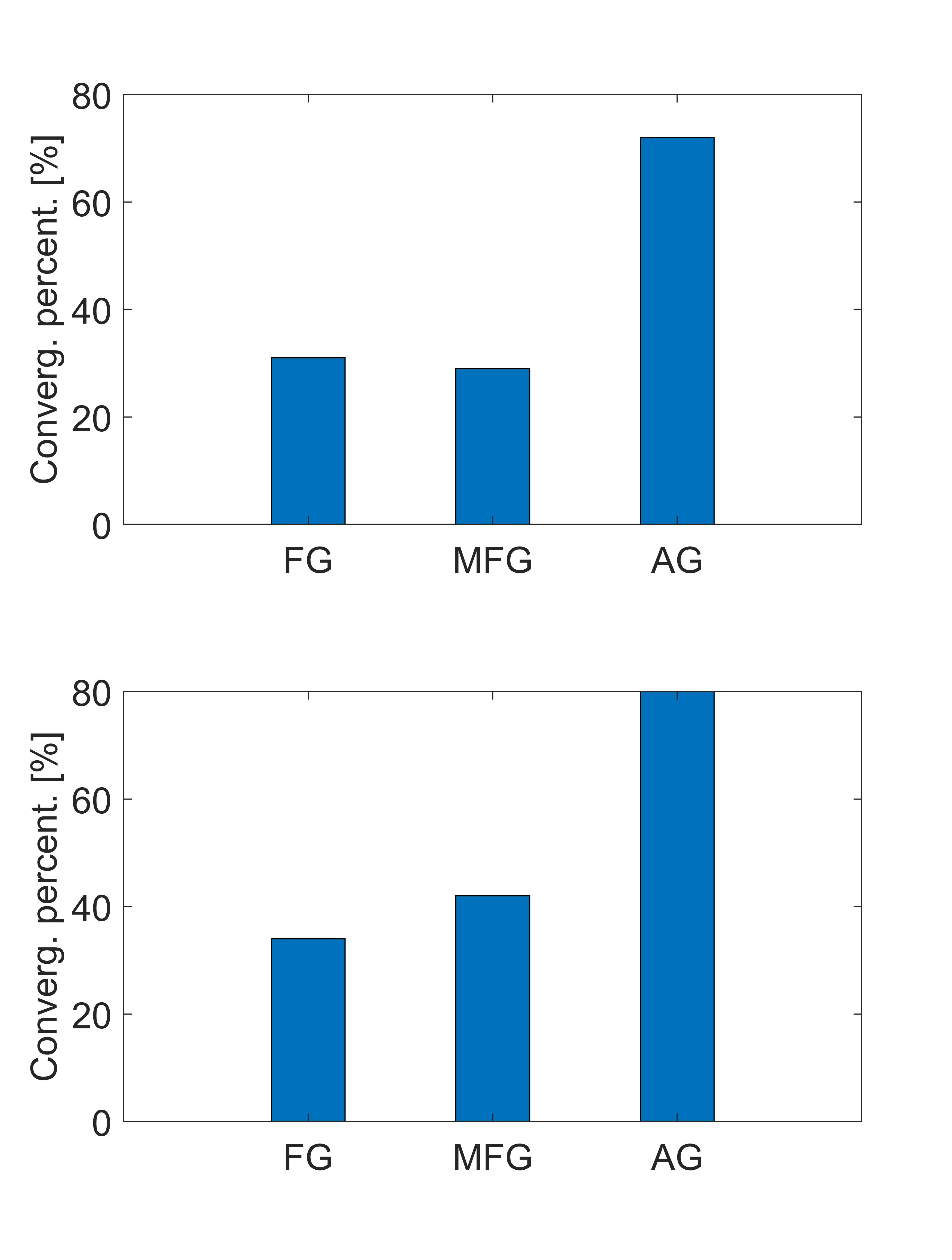
(b) Convergence % $\uparrow$

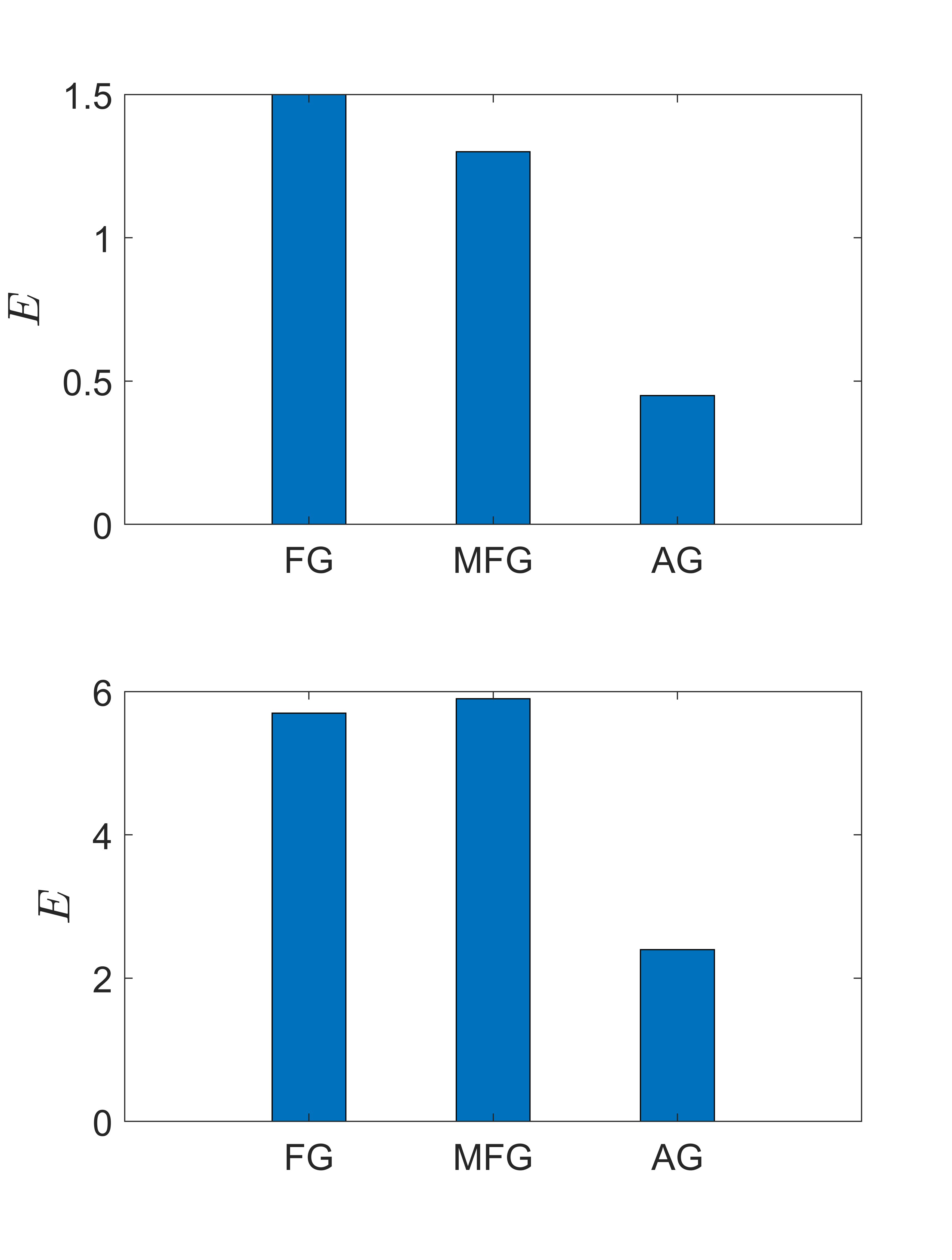
(c) Average cost $E\downarrow$

Figure 9: Results of the proposed adaptive approach (AG) compared with the traditional genetic approach (FG) and the modified traditional genetic approach (MFG). The upper row shows the plot for the UAV model, while the bottom one is for the vehicle model. The proposed AG approach achieves a 39%-53% reduction in the average computational time compared to other approaches. Additionally, AG converges to the optimal solution with percentages of 72% and 80% of all iterations for the UAV and vehicle, respectively. In contrast, the FG approach yields 31% and 34%, and MFG yields 29% and 42%. The higher percentage of cycles that yielded optimal solutions with AG reflects its superior performance. Specifically, AG outperformed other approaches in $E$ with percentages of 54% and 67% for the UAV and vehicle models, respectively.

As shown in Fig. 9, the proposed AG approach reduces the average computational time significantly compared with both FG and MFG approaches. Specifically, it reduces the computations by 39% and 53% for the UAV and the vehicle, respectively, as shown in Fig. 9 (a). This reduction in computational time results from exploring less search space by the proposed approach due to its estimation of the optimal $\boldsymbol{\Delta}_{c}$. Therefore, it converges to the optimal solution in a shorter time. Additionally, the proposed AG approach outperforms the other approaches in terms of the percentage of the cycles that each approach converges to the optimal solution before the termination of the cycle’s time, as shown in Fig. 9 (b). The proposed AG approach shows superior percentages of 72% and 80% for the UAV and the vehicle models, respectively. This higher percentage of cycles that yielded optimal solutions with AG further reflects its superior performance over other approaches, as it appears from its reported $E$ in Fig. 9 (c). Specifically, AG outperforms other approaches in $E$ with percentages 54% and 67% for the UAV and vehicle models, respectively. The reason is that the proposed AG approach explores less search space due to its estimation of the optimal margin, and thus, it converges to the optimal solution more often.

In contrast, the FG approach produces the optimal solution for the UAV and the vehicle in only 31% and 34% of all cycles, respectively. Furthermore, although MFG utilizes a proportion of the population from the best suboptimal solutions obtained in the previous cycle, it provides little benefit. Specifically, the MFG approach produces the optimal solution for the UAV and the vehicle in only 29% and 42% of all cycles, respectively. The reason for this is that the MFG approach forms its population with a proportion of time-shifted versions of the best solutions in the last generation of genetic optimization in the previous control cycle, which may not be suitable in the current cycle due to the unexpected disturbances and noises introduced to the system. This differs from the proposed AG approach, which estimates the control inputs in each cycle and ensures that the solutions are generated only around the optimal solution from the previous cycle within the estimated search space. We can make the same conclusion about the results of the MFG when changing its proportions into 60% and 40%, as shown in Sec. S.IV in the supplementary material.

To further show the effectiveness of the proposed AG approach in reducing the population size $p_{c}$ in the conducted experiments, we plot a histogram for $p_{c}$ in all cycles for both the UAV and the vehicle models in Fig. 10 (a) and (b), respectively. The figure shows that the AG approach exhibits variable $p_{c}$ resulting from its adaptive estimation for the optimal $\boldsymbol{\Delta}_{c}$. Additionally, $p_{c}$ has small values most of the time, as shown by the histograms, which results in a significant reduction in computations. On the other hand, the FG and MFG approaches utilize a fixed, large population to cover the large search space that arises from the physical margins of the control inputs, which results in unnecessary computations.

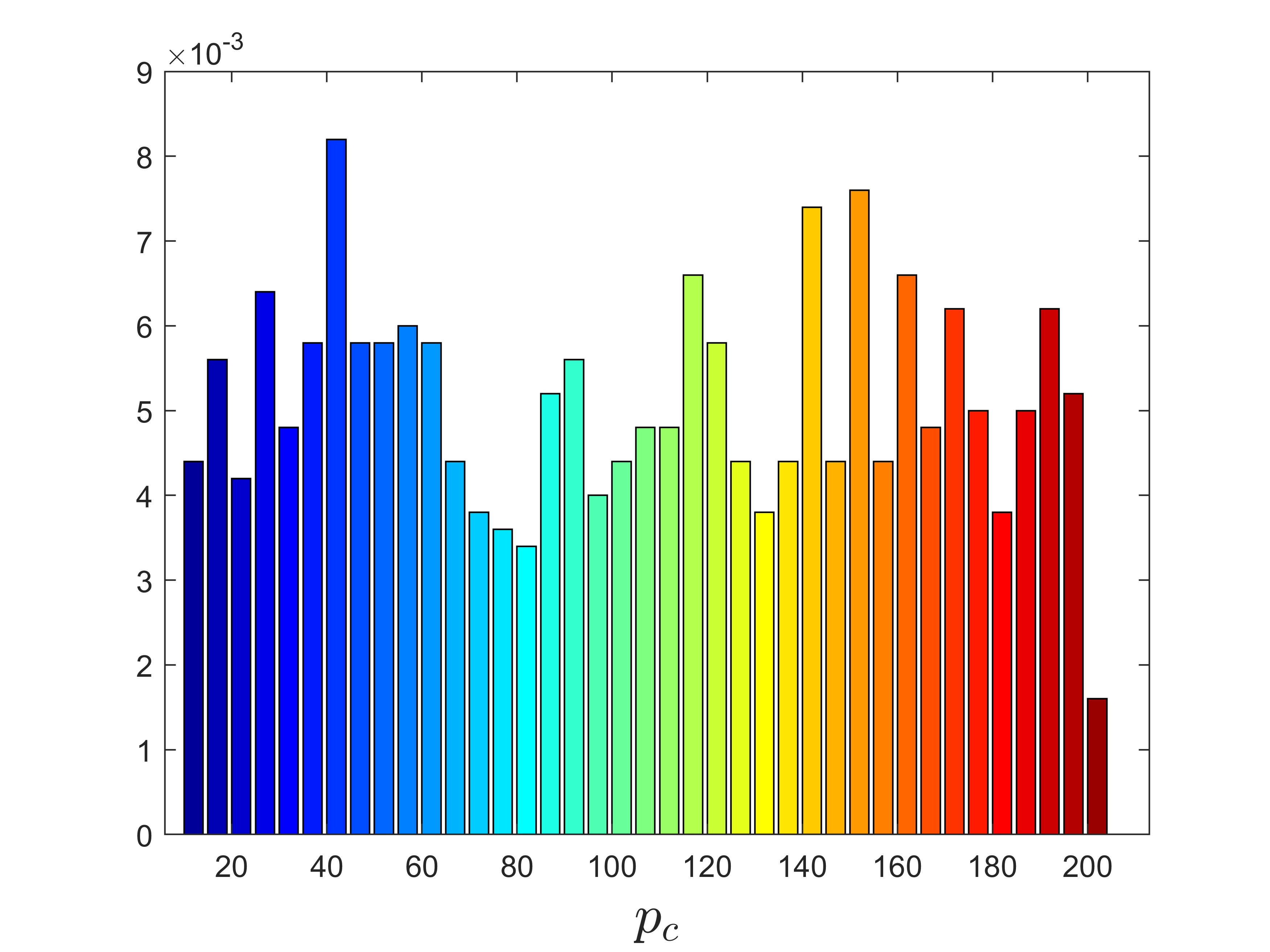
(a) UAV

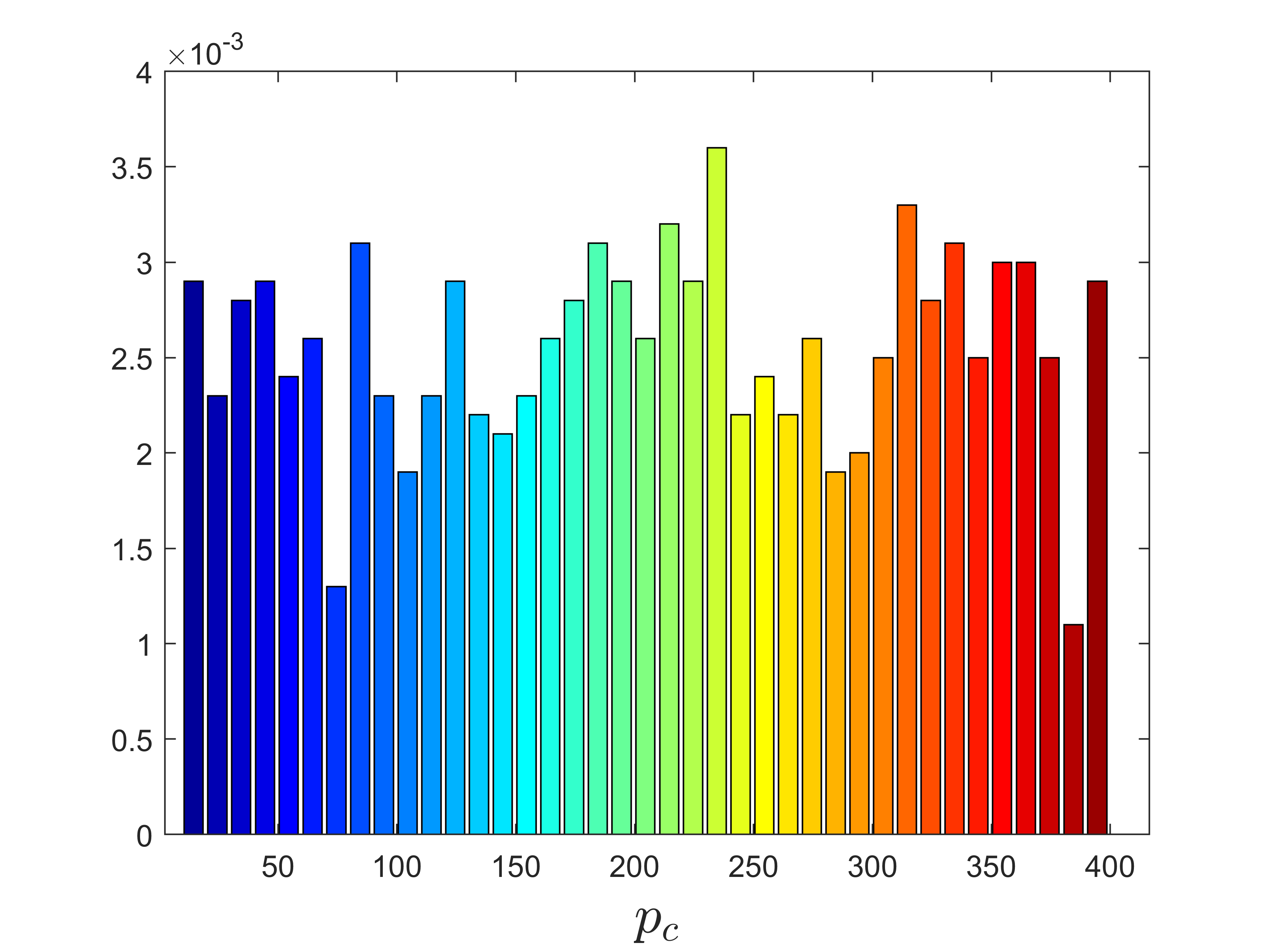
(b) Vehicle

Figure 10: Histogram of the population size $p_{c}$ in all cycles for both the UAV and the vehicle models for the proposed AG approach. The AG approach utilizes a variable population size according to the estimated margin, instead of employing a fixed, large population size in all control cycles, which results in a significant reduction in computations.

V-C Parameter sensitivity analysis

As mentioned in Sec. IV, the threshold $\epsilon$ is set depending on the specific application and the desired level of optimality. This subsection investigates the impact of $\epsilon$ on our proposed AG approach’s performance and computational time. Specifically, for various values of $\epsilon$, we calculate the average cost $E$, average computational time, and the percentage of the cycles that converge to the optimal solution before the termination of the cycle’s time for different settings of $\epsilon$. The results are presented in Fig. 11, where the top row displays the results for the UAV model, and the bottom row represents the vehicle model. We plot the average computational time, the convergence percentage, and $E$ in Fig. 11 (a), (b), and (c), respectively.

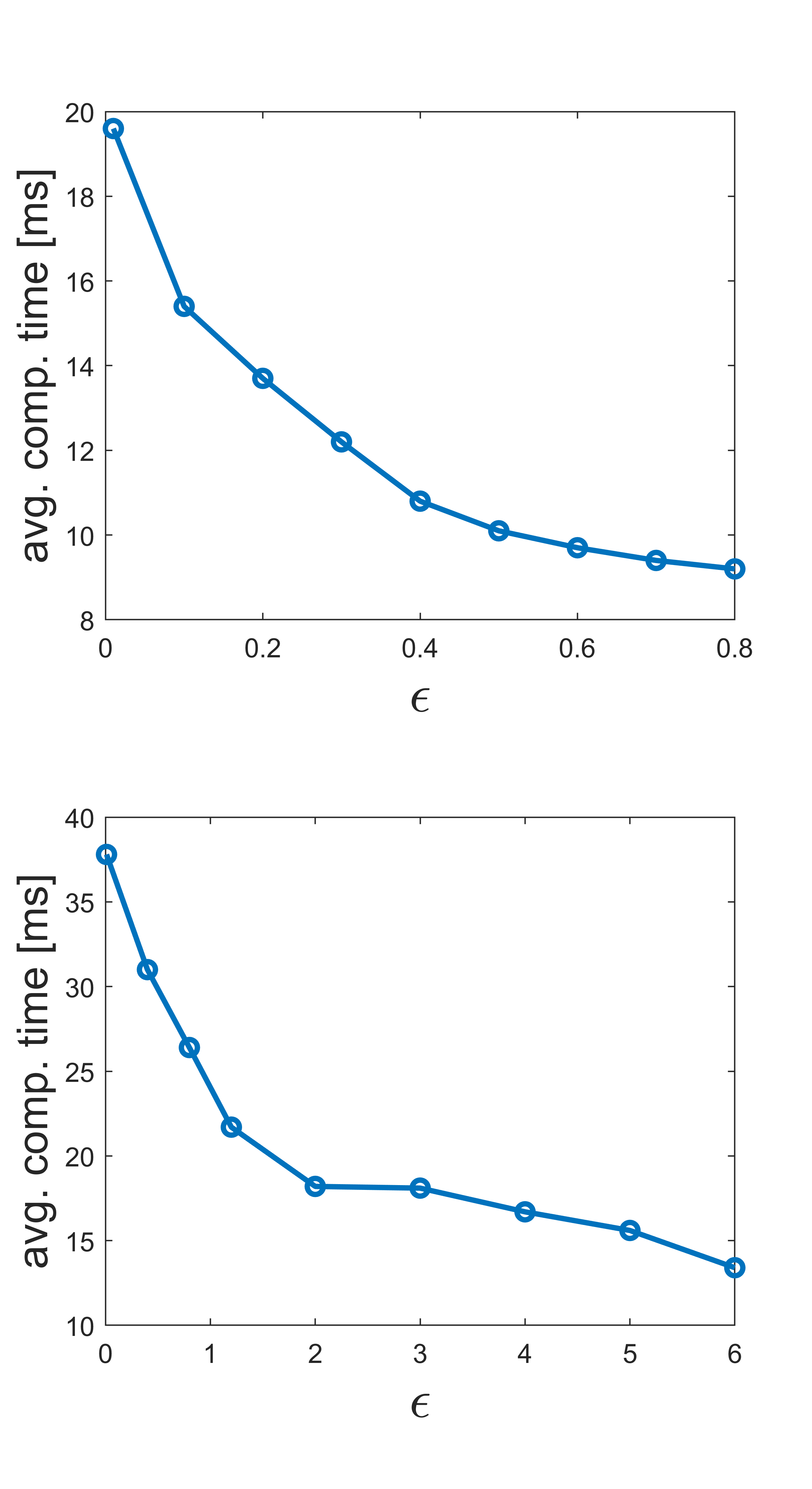
(a) Comp. time

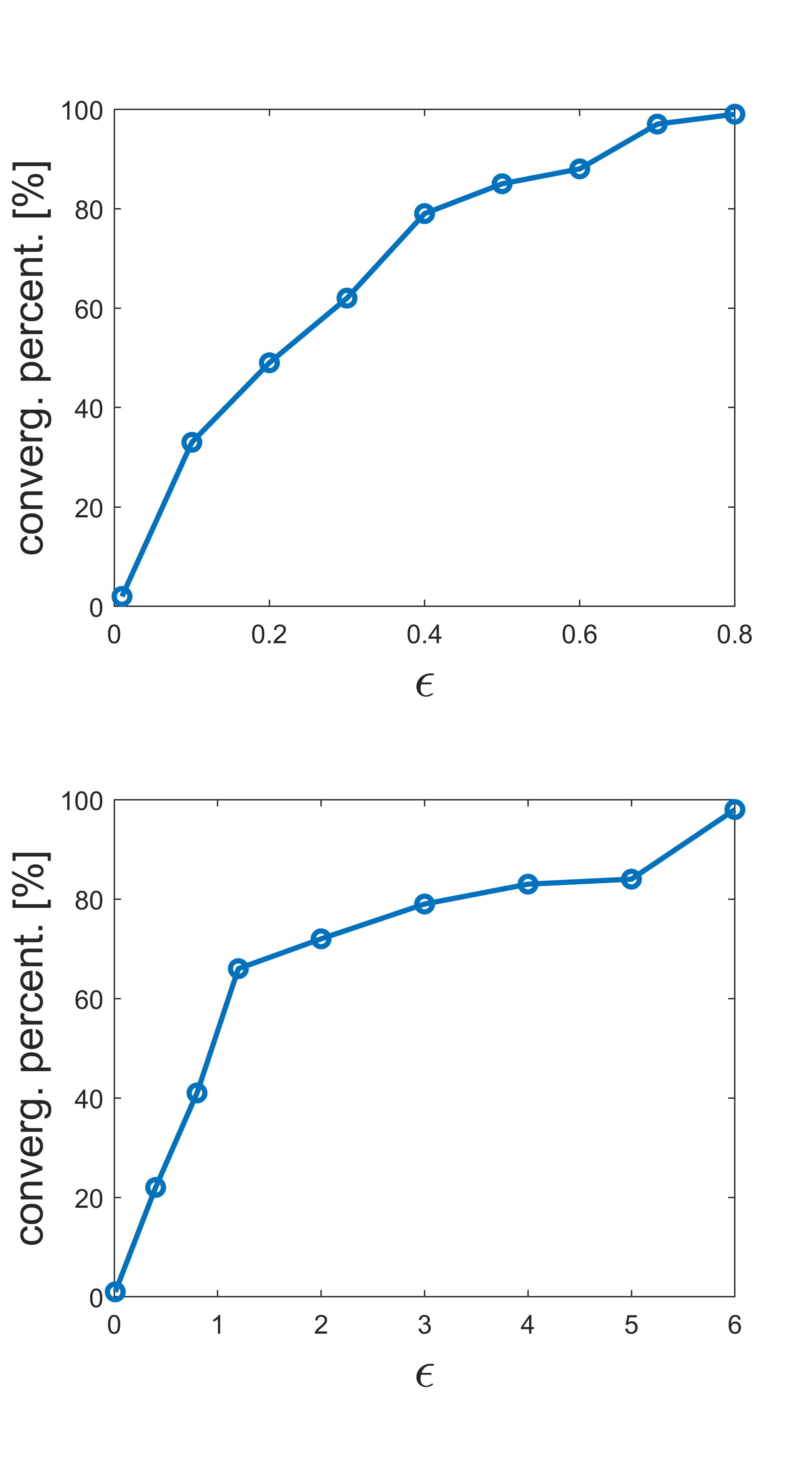
(b) Convergence

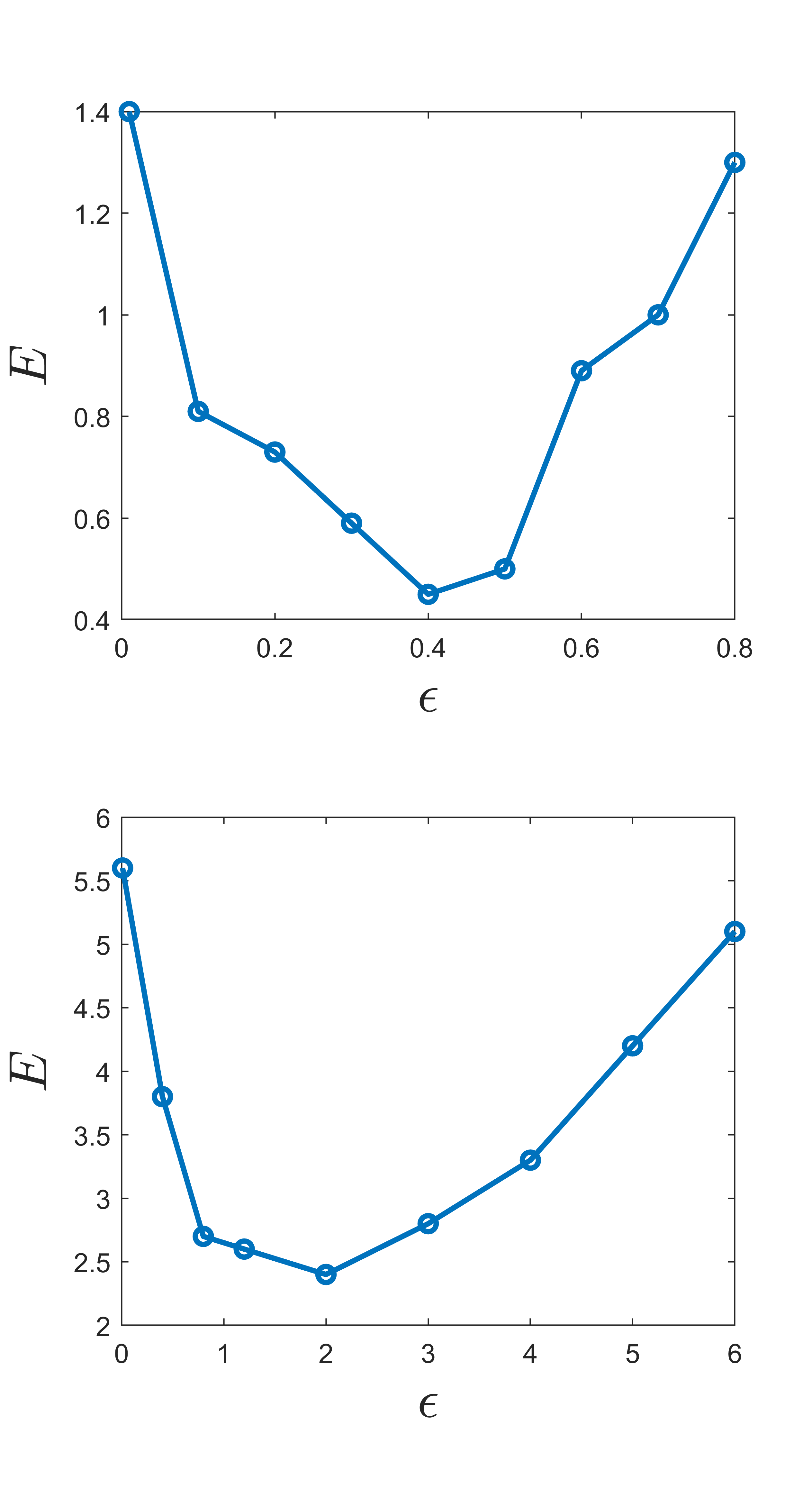
(c) Average cost $E$

Figure 11: Parameter sensitivity analysis of $\epsilon$. The top and bottom rows show the results for the UAV and vehicle models, respectively. Increasing $\epsilon$ leads to a reduction in the average computational time and an increase in the convergence percentage. Additionally, increasing $\epsilon$ reduces $E$ initially, i.e., enhances the performance. However, there is a point at which further increasing $\epsilon$ causes diminishing returns, and the performance worsens because the AG approach, in this case, may set the margin around less precise optimal solutions, allowing errors in the control inputs to accumulate with the progression of control cycles.

As shown in Fig. 11 (a) and (b), increasing $\epsilon$ reduces the average computational time and, at the same time, increases the percentage of the cycles that the approach converges to the optimal solution before the termination of the cycle’s time. Increasing $\epsilon$ makes the genetic optimization treat any solution that costs less than $\epsilon$ as an optimal solution. Thus it terminates the optimization’s iterations early and counts this termination as a converges to the optimal solution before the termination of the cycle’s time. Therefore, the average computational time decreased, and the convergence percentage increased, as shown in Fig. 11 (a) and (b).

For the average cost $E$, increasing $\epsilon$ reduces $E$ initially, i.e., enhances the performance, as shown in Fig. 11 (c). However, there is a point at which further increasing $\epsilon$ causes diminishing returns, and the performance gets worse. This is because, in our proposed AG approach, we set the optimal search space to be around the previously found solution if it is optimal, i.e., its cost is less than $\epsilon$. Otherwise, the optimal search space is equal to the physical margin. Thus, increasing the value of $\epsilon$ enhances the probability of setting the margin to be around the previously found solution but leads to diminishing returns, as the AG may set the margin around less precise optimal solutions, allowing errors in the control inputs to accumulate with the progression of control cycles. It is worth noting that, in some control scenarios, obtaining quick non-optimal control inputs is more critical than obtaining optimal ones from the NMPC. These scenarios occur when running the NMPC on a platform with limited computational resources or when a short control cycle is allowed. In these cases, the threshold $\epsilon$ must be set to larger values to reduce computations, as adaptively setting $\boldsymbol{\Delta}_{c}$ reduces the search space dramatically compared to the system’s physical constraints.

VI Conclusion

This paper proposes a novel approach to accelerate the genetic optimization of nonlinear model predictive control (NMPC) by learning optimal search space size. The proposed approach trains a regression model to predict the best smallest search space in every control cycle to increase the likelihood of obtaining optimal control inputs within the shortest computational time. This approach was evaluated on two nonlinear systems and compared with two other genetic-based NMPC techniques implemented on the GPU of a Nvidia^™ Jetson TX2 embedded platform in a processor-in-the-loop (PIL) fashion. The results showed that the proposed approach outperformed other approaches in terms of computational time, achieving a 39-53% reduction in computational time. Additionally, it increases the percentage of convergence to the optimal control inputs within the cycle’s time by 48-56%, resulting in a significant performance enhancement.

For future research, there are several potential directions based on the findings of this study. One possible direction is to integrate the proposed approach with the adaptive horizon estimation approach proposed in [27] to improve the overall performance of NMPC. Another direction is to apply the proposed approach to other real-time applications in the industry, where optimizing control inputs with high accuracy and low computational cost is critical.

References

- [1] C. E. Garcia, D. M. Prett, and M. Morari, “Model predictive control: Theory and practice-A survey,” Automatica, vol. 25, no. 3, pp. 335–348, 1989.
- [2] R. Gelleschus, M. Böttiger, P. Stange, and T. Bocklisch, “Comparison of optimization solvers in the model predictive control of a PV-battery-heat pump system,” Energy Procedia, vol. 155, pp. 524–535, 2018.
- [3] O. Kramer, Genetic algorithm essentials, ser. Studies in Computational Intelligence. New York: Springer, 2017.
- [4] R. A. Sarker and M. A. Kazi, “Population size, search space and quality of solution: An experimental study,” in The 2003 Congress on Evolutionary Computation, 2003. CEC’03., vol. 3. IEEE, 2003, pp. 2011–2018.
- [5] A. Hassanat, K. Almohammadi, E. Alkafaween, E. Abunawas, A. Hammouri, and V. S. Prasath, “Choosing mutation and crossover ratios for genetic algorithms—A review with a new dynamic approach,” Information, vol. 10, no. 12, p. 390, 2019.
- [6] L. Bayas-Jiménez, F. J. Martínez-Solano, P. L. Iglesias-Rey, and D. Mora-Meliá, “Search space reduction for genetic algorithms applied to drainage network optimization problems,” Water, vol. 13, no. 15, p. 2008, 2021.
- [7] D. Franklin, “Nvidia Jetson TX2 technical specifications,” https://developer.nvidia.com/zh-cn/blog/jetson-tx2-delivers-twice-intelligence-edge/, 2023, [Accessed: April 1, 2023].
- [8] S. Arrigoni, F. Braghin, and F. Cheli, “MPC trajectory planner for autonomous driving solved by genetic algorithm technique,” Vehicle system dynamics, vol. 60, no. 12, pp. 4118–4143, 2022.
- [9] X. Du, K. K. K. Htet, and K. K. Tan, “Development of a genetic-algorithm-based nonlinear model predictive control scheme on velocity and steering of autonomous vehicles,” IEEE Transactions on Industrial Electronics, vol. 63, no. 11, pp. 6970–6977, 2016.
- [10] S. Samsam and R. Chhabra, “Nonlinear model predictive control of J2-perturbed impulsive transfer trajectories in long-range rendezvous missions,” Aerospace Science and Technology, vol. 132, p. 108046, 2023.
- [11] P. Hyatt and M. D. Killpack, “Real-time evolutionary model predictive control using a graphics processing unit,” in 2017 IEEE-RAS 17th International Conference on Humanoid Robotics (Humanoids). IEEE, 2017, pp. 569–576.
- [12] V. Ranković, J. Radulović, N. Grujovic, and D. Divac, “Neural network model predictive control of nonlinear systems using genetic algorithms,” International Journal of Computers, Communications and Control, 2012.
- [13] H. Zhu, G. Zhao, L. Sun, and K. Y. Lee, “Nonlinear predictive control for a boiler–turbine unit based on a local model network and immune genetic algorithm,” Sustainability, vol. 11, no. 18, p. 5102, 2019.
- [14] W. Chen, X. Li, and M. Chen, “Suboptimal nonlinear model predictive control based on genetic algorithm,” in 2009 Third international symposium on intelligent information technology application workshops. IEEE, 2009, pp. 119–124.
- [15] G. Wang, Q.-S. Jia, J. Qiao, J. Bi, and M. Zhou, “Deep learning-based model predictive control for continuous stirred-tank reactor system,” IEEE Transactions on Neural Networks and Learning Systems, vol. 32, no. 8, pp. 3643–3652, 2020.
- [16] S. K. Sharma and R. Sutton, “An optimised nonlinear model predictive control based autopilot for an uninhabited surface vehicle,” IFAC Proceedings Volumes, vol. 46, no. 10, pp. 73–78, 2013.
- [17] S. Sharma and R. Sutton, “A genetic algorithm based nonlinear guidance and control system for an uninhabited surface vehicle,” Journal of Marine Engineering & Technology, vol. 12, no. 2, pp. 29–40, 2013.
- [18] E. Picotti, L. Facin, A. Beghi, M. Nishimura, Y. Tezuka, F. Ambrogi, and M. Bruschetta, “Data-driven tuning of a NMPC controller for a virtual motorcycle through genetic algorithm,” in 2022 IEEE Conference on Control Technology and Applications (CCTA). IEEE, 2022, pp. 1222–1227.
- [19] D. Yu, F. Deng, H. Wang, X. Hou, H. Yang, and T. Shan, “Real-time weight optimization of a nonlinear model predictive controller using a genetic algorithm for ship trajectory tracking,” Journal of Marine Science and Engineering, vol. 10, no. 8, p. 1110, 2022.
- [20] T. Yasini, J. Roshanian, and A. Taghavipour, “Improving the low orbit satellite tracking ability using nonlinear model predictive controller and genetic algorithm,” Advances in Space Research, vol. 71, no. 6, pp. 2723–2732, 2023.
- [21] T. Luukkonen, “Modelling and control of quadcopter,” Independent research project in applied mathematics, Espoo, vol. 22, no. 22, 2011.
- [22] J. Kong, M. Pfeiffer, G. Schildbach, and F. Borrelli, “Kinematic and dynamic vehicle models for autonomous driving control design,” in 2015 IEEE intelligent vehicles symposium (IV). IEEE, 2015, pp. 1094–1099.
- [23] W. Naeem, R. Sutton, J. Chudley, F. Dalgleish, and S. Tetlow, “A genetic algorithm-based model predictive control autopilot design and its implementation in an autonomous underwater vehicle,” Proceedings of the Institution of Mechanical Engineers, Part M: Journal of Engineering for the Maritime Environment, vol. 218, no. 3, pp. 175–188, 2004.
- [24] K. Jebari and M. Madiafi, “Selection methods for genetic algorithms,” International Journal of Emerging Sciences, vol. 3, no. 4, pp. 333–344, 2013.
- [25] T. Joachims, “A support vector method for multivariate performance measures,” in Proceedings of the 22nd international conference on Machine learning, 2005, pp. 377–384.
- [26] J. Chorowski, J. Wang, and J. M. Zurada, “Review and performance comparison of SVM-and ELM-based classifiers,” Neurocomputing, vol. 128, pp. 507–516, 2014.
- [27] E. Mostafa, H. A. Aly, and A. Elliethy, “Fast adaptive regression-based model predictive control,” accepted for publication in Control Theory and Technology May. 2023.