Pulsar timing residual induced by ultralight tensor dark matter

Abstract

Ultralight boson fields, with a mass around $10^{-23}\text{eV}$, are promising candidates for the elusive cosmological dark matter. These fields induce a periodic oscillation of the spacetime metric in the nanohertz frequency band, which is detectable by pulsar timing arrays. In this paper, we investigate the gravitational effect of ultralight tensor dark matter on the arrival time of radio pulses from pulsars. We find that the pulsar timing signal caused by tensor dark matter exhibits a different angular dependence than that by scalar and vector dark matter, making it possible to distinguish the ultralight dark matter signal with different spins. Combining the gravitational effect and the coupling effect of ultralight tensor dark matter with standard model matter provides a complementary way to constrain the coupling parameter $\alpha$. We estimate $\alpha\lesssim 10^{-6}\sim 10^{-5}$ in the mass range $m<5\times 10^{-23}\mathrm{eV}$ with current pulsar timing array.

I Introduction

Numerous cosmological observations (Rubin et al., 1980, 1982; Faber and Jackson, 1976; Massey et al., 2010) have provided overwhelming support for the existence of dark matter, and precise analyses of cosmic microwave background (CMB) (Aghanim et al., 2020) in particular have estimated the fraction of dark matter in the total energy of the Universe. However, the nature and properties of dark matter, such as its composition and interaction with the Standard Model (SM), remain mysterious. There are plenty dark matter candidates (Bertone et al., 2005; Feng, 2010; Bertone and Tait, 2018), from tiny axion-like particles with mass around $10^{-22}\,\mathrm{\rm{eV}}$ (Marsh, 2016) to planet-sized massive compact halo objects (MACHOs) of $m\sim M_{\odot}$ (Alcock et al., 2000). Among the bunch candidates, the weakly interactive massive particles (WIMPs) are expected to be highly desirable. However, despite considerable efforts in searching for them, no signal of WIMPs has yet been observed (Schumann, 2019).

In recent years, ultralight dark matter (ULDM) with a mass around $10^{-23}\,\mathrm{\rm{eV}}$ has attracted wide attention (Hu et al., 2000; Hui et al., 2017). The ULDM is assumed to be condensed before inflation and oscillates coherently when its mass is larger than the Hubble scale (Fox et al., 2004). On the one hand, ULDM moves at a non-relativistic speed, retaining the advantages of traditional cold dark matter to explain the large-scale structure of galaxies. On the other hand, its large de Broglie wavelength can suppress the structure on small scales, providing feasible solutions to the puzzles encountered by the traditional cold dark matter (Hui et al., 2017; Niemeyer, 2019), such as the core-cusp problem Gentile et al. (2004); de Blok (2010) and missing-satellites problem Moore et al. (1999); Klypin et al. (1999).

ULDM has been traditionally represented by scalar (Hu et al., 2000; Khmelnitsky and Rubakov, 2014; Hui et al., 2017) or pseduo-scalar fields (spin-0) such as axion-like particles (Arvanitaki et al., 2010; Hlozek et al., 2015; Payez et al., 2015; Ivanov et al., 2019). However, fields with higher spins, such as the massive vector fields (spin-1), can also act as alternative candidates for ULDM. Although ULDM candidates with different spins share many similarities in the cosmological phenomena, each possesses specific features. For instance, the massive vector particles can interact with SM particles if they are gauge bosons for $U(1)_{B}$ (“B” refers to baryon) or $U(1)_{B-L}$ (“L” refers to lepton) symmetry (Pierce et al., 2018), and their multiple polarization modes may cause anisotropies in certain experiments (Nomura et al., 2020).

Recently, massive tensor fields (spin-2) have been proposed as another viable candidate for dark matter (Aoki and Mukohyama, 2016; Babichev et al., 2016a, b; Aoki and Maeda, 2018). The tensor ULDM can be naturally predicted by a ghost-free bimetric theory (Hassan and Rosen, 2012) in some mass range (Marzola et al., 2018). This theory has two mass eigenstates at the linearized level: a massless spin-2 field $G_{\mu\nu}$ and a massive spin-2 field $M_{\mu\nu}$. At nonlinear levels, the expansion of the action (Babichev et al., 2016a, b; Marzola et al., 2018) reveals that the self-interaction terms of the massless graviton $G_{\mu\nu}$ exactly match the Einstein-Hilbert structure. Meanwhile, the massive mode gravitates with the same strength as SM matter. But it lacks terms that combine $M_{\mu\nu}$ in linear order and $G_{\mu\nu}$ in any order. As a result, the terms with $G_{\mu\nu}$ can be partially resumed up to an effective background $g_{\mu\nu}$. In contrast, the massive fluctuation $M_{\mu\nu}$ can be treated as a propagating massive spin-2 field on the background $g_{\mu\nu}$.

The ULDM can leave imprints on cosmological and astrophysical observables. Its mass range and properties have been explored by many experiments, such as CMB (Hlozek et al., 2015; Poulin et al., 2018), Lyman-$\alpha$ (Iršič et al., 2017, 2017), non-observation of superradiance (Ünal et al., 2021), secular variations in binary-pulsar orbital parameters (Armaleo et al., 2020a; Blas et al., 2020), etc. In particular, for dark matter fields with a mass around $10^{-23}\,\mathrm{\rm{eV}}$, pulsar timing arrays (PTAs) provide a powerful tool for exploring both its gravitational and non-gravitational properties (Khmelnitsky and Rubakov, 2014; Porayko and Postnov, 2014; Porayko et al., 2018; Kato and Soda, 2020; Nomura et al., 2020; Xue et al., 2022; Wu et al., 2022; Armaleo et al., 2020b). A PTA consists of a set of millisecond pulsars for which the arrival time of the emitted radio pulses are monitored with high precision for decades (Sazhin, 1978; Detweiler, 1979; Foster and Backer, 1990), recording the spacetime disturbances in the nanohertz range. The coherent motion of ULDM carrying energy and momentum induces nontrivial oscillations of the metric (Khmelnitsky and Rubakov, 2014; Nomura et al., 2020), which can leave a mark on the timing residuals of PTA, known as the “gravitational effect”. Additionally, if ULDM interacts with SM particles, it can lead to pulsar spin fluctuations and reference clock shifts due to the induced variations in fundamental constants of the SM (Kaplan et al., 2022) or can exert periodic forces on both the pulsar and Earth, resulting in relative displacements between them (Xue et al., 2022). These effects are called the “coupling effect” and can cause timing residuals.

The specific form of the pulsar timing signal depends on the spin of ULDM. One unique aspect of tensor dark matter is that it naturally couples to SM fields without manually adding a fifth force to mimic the modification of gravity. This coupling effect on the PTA has been investigated in previous studies (Armaleo et al., 2020b; Sun et al., 2022; Unal et al., 2022). In our present work, we will instead focus on the gravitational effect of the tensor dark matter on PTA, which we expect to be different from that of the scalar and vector dark matter because of possessing more polarization modes. The paper is organized as follows. In Section II, we show the time-dependent spacetime perturbations induced by the oscillating tensor ULDM. In Section III, we derive the pulsar timing residuals induced by the tensor ULDM from the gravitational effect. We also discuss the constraints that can be inferred from current data and compare the gravitational and coupling effects in IV. In Section V, we summarize the results.

II Metric perturbations induced by tensor ULDM

The action for a massive spin-2 filed $M_{\mu\nu}$ propagating on a background $g_{\mu\nu}$ can be formally written as (Marzola et al., 2018)

$$S=\frac{M_{\rm{P}}^{2}}{2}\int d^{4}x\sqrt{-g}R(g)+\int d^{4}x\sqrt{-g}{\cal{L}}_{\rm{FP}}^{(2)}(M)+{\cal{O}}(M_{\mu\nu}^{3}),$$ (1)

where $M_{\rm{P}}$ is the reduced Planck mass, and ${\cal{L}}_{\rm{FP}}^{(2)}(M)$ is the quadratic Fierz-Pauli Lagrangian,

$${\cal{L}}_{\rm{FP}}^{(2)}(M)=\frac{1}{8}\left[-\nabla_{\rho}M_{\mu\nu}\nabla^{\rho}M^{\mu\nu}+2\nabla_{\rho}M_{\mu\nu}\nabla^{\nu}M^{\mu\rho}-2\nabla_{\nu}M^{\mu\nu}\nabla_{\mu}M+\nabla^{\mu}M\nabla_{\mu}M+m^{2}(M^{2}-M_{\mu\nu}M^{\mu\nu})\right]$$ (2)

with the trace $M=M_{\,\,\,\mu}^{\mu}$. The cosmic expansion is negligible on galactic scales, so we treat the background to be flat. The equation of motion of the tensor fields can be derived from the action Eq. (1) by taking the variation with respect to $M_{\mu\nu}$,

$$\square M^{\mu\nu}-(\partial^{\mu}\partial_{\rho}M^{\nu\rho}+\partial^{\nu}\partial_{\rho}M^{\mu\rho})+\eta^{\mu\nu}\partial_{\rho\sigma}M^{\rho\sigma}+\partial^{\mu\nu}M-\eta^{\mu\nu}\square M=m^{2}(M^{\mu\nu}-\eta^{\mu\nu}M).$$ (3)

Applying $\partial_{\mu}$ to both sides of Eq. (3), the left-hand side gives zero identically, so we obtain

$$m^{2}\partial_{\mu}(M^{\mu\nu}-\eta^{\mu\nu}M)=0.$$ (4)

Further, taking the trace of both sides of Eq. (3), we get

$$2\partial_{\mu}\partial_{\nu}(M^{\mu\nu}-\eta^{\mu\nu}M)=-3m^{2}M.$$ (5)

With Eq. (4) and Eq. (5), we can rewrite Eq. (3) into a set of equations for a massive tensor field in the standard form

$$M = 0,$$ (6)

$$\partial_{\mu}M^{\mu\nu} = 0,$$ (7)

$$(\square-m^{2})M^{\mu\nu} = 0.$$ (8)

Now we consider the scenario where the spin-2 fields with an ultralight mass act as the dark matter following the discussion in Refs. (Khmelnitsky and Rubakov, 2014; Nomura et al., 2020; Armaleo et al., 2020b). For ULDM with the typical mass $m\sim 10^{-23}\rm{eV}$ and the typical velocity in the galaxy $v\sim 10^{-3}$, the occupation number can be estimated to be as high as $10^{95}$, allowing us to treat the ultralight field as a classical wave. The wave is characterized by a typical wave number $k=mv$ and frequency $\omega\approx m+mv^{2}/2\approx m$ due to the non-relativistic velocity. Additionally, the de Broglie wavelength of the ULDM can be calculated as

$$\lambda_{\rm{dB}}=\frac{2\pi}{k}\approx 4{\rm{kpc}}\left(\frac{10^{-23}{\rm{eV}}}{m}\right)\left(\frac{10^{-3}}{v}\right),$$ (9)

indicating the spin-2 field oscillates coherently with a monochromatic frequency determined by its mass on the scale of $\lambda_{\rm{dB}}$.

We return to Eqs. (6-8). Note that the constraint in Eq. (7) indicates that $M^{00}$ is suppressed by the order of $k/m=v\sim 10^{-3}$ compared to $M^{0j}$, while $M^{0j}$ is suppressed by the same order compared to $M^{ij}$. Thus, we can neglect all the time components $M^{0\mu}$. Since the remains six spatial components $M_{ij}$ are subject to the traceless constraint in Eq. (6), the solution to Eq. (8) is given by

$$M_{ij}(t,\mathbf{x})=A(\mathbf{x})\cos(mt+\alpha(\mathbf{x}))\epsilon_{ij}.$$ (10)

We have neglected the spatial derivatives when solving the equation but retain the spatial dependence of the amplitude $A(\mathbf{x})$ and the phase $\alpha(\mathbf{x})$. The symmetric, traceless matrix $\epsilon_{ij}$ with a unit norm encoding the five free degrees of freedom of the massive spin-2 fields is (Armaleo et al., 2020a),

$$\begin{gathered}\epsilon_{ij}=\frac{1}{\sqrt{2}}\begin{pmatrix}\epsilon_{\rm{T}}\cos\chi-\epsilon_{\rm{S}}/\sqrt{3}&\epsilon_{\rm{T}}\sin\chi&\epsilon_{\rm{V}}\cos\xi\\ \epsilon_{\rm{T}}\sin\chi&-\epsilon_{\rm{T}}\cos\chi-\epsilon_{\rm{S}}/\sqrt{3}&\epsilon_{\rm{V}}\sin\xi\\ \epsilon_{\rm{V}}\cos\xi&\epsilon_{\rm{V}}\sin\xi&2\epsilon_{\rm{S}}/\sqrt{3}\end{pmatrix}\end{gathered}.$$ (12)

The amplitude parameters $\epsilon_{\rm{S}}$, $\epsilon_{\rm{V}}$, and $\epsilon_{\rm{T}}$, satisfying $\epsilon_{\rm{S}}^{2}+\epsilon_{\rm{V}}^{2}+\epsilon_{\rm{T}}^{2}=1$, represent the ratios of the scalar, vector, and tensor sector of the massive spin-2 fields, respectively. Meanwhile, the angle parameters $\xi$ and $\chi$ determine the azimuthal direction of the helicity-$\pm 1$ and helicity-$\pm 2$ modes, respectively.

Now let’s focus on the metric perturbation induced by the oscillating fields. Using the definition of energy-momentum from the matter fields,

$$T_{\mu\nu}=\frac{-2}{\sqrt{-g}}\frac{\delta S}{\delta g^{\mu\nu}},$$ (13)

the energy-momentum of the massive spin-2 fields in a flat background is given by,

$$T_{\mu\nu}=-\frac{1}{8}\left[\eta_{\mu\nu}\left(\partial_{\lambda}M^{\gamma\delta}\partial^{\lambda}M_{\gamma\delta}+m^{2}M^{\gamma\delta}M_{\gamma\delta}\right)-2\partial_{\mu}M_{\gamma\delta}\partial_{\nu}M^{\gamma\delta}-4\partial_{\lambda}M_{\mu\delta}\partial^{\lambda}M^{\delta}_{\,\,\nu}-4m^{2}M_{\mu\delta}M^{\delta}_{\,\,\nu}\right].$$ (14)

with the corresponding time-dependent energy density

$$T_{00}=\frac{1}{8}m^{2}A(\mathbf{x})^{2}=\rho_{\rm{TF}}(\mathbf{x}),$$ (15)

and the oscillating spatial components

$$\begin{gathered}T_{ij}=\frac{1}{24}\!m^{2}\!A(\mathbf{x})^{2}\!\cos(2mt\!+\!2\alpha(\mathbf{x}))\qquad\qquad\qquad\qquad\qquad\qquad\qquad\qquad\qquad\qquad\qquad\qquad\qquad\qquad\qquad\qquad\qquad\qquad\\ \times\begin{pmatrix}\!-(\epsilon_{\rm{S}}^{2}\!+4\sqrt{3}\epsilon_{\rm{S}}\epsilon_{\rm{T}}c_{\chi}\!-3(\epsilon_{\rm{T}}^{2}\!+\epsilon_{\rm{V}}^{2}c_{2\xi}))&\!-4\sqrt{3}\epsilon_{\rm{S}}\epsilon_{\rm{T}}s_{\chi}\!+3\epsilon_{\rm{V}}^{2}s_{2\xi}&2\epsilon_{\rm{V}}(\sqrt{3}\epsilon_{\rm{S}}c_{\xi}\!+3\epsilon_{\rm{T}}c_{\chi-\xi})\\ \!-4\sqrt{3}\epsilon_{\rm{S}}\epsilon_{\rm{T}}s_{\chi}\!+3\epsilon_{\rm{V}}^{2}s_{2\xi}&-(\epsilon_{\rm{S}}^{2}\!-4\sqrt{3}\epsilon_{\rm{S}}\epsilon_{\rm{T}}c_{\chi}\!-3\epsilon_{\rm{T}}^{2}\!+3\epsilon_{\rm{V}}^{2}c_{2\xi})&2\epsilon_{\rm{V}}(\sqrt{3}\epsilon_{\rm{S}}s_{\xi}\!+3\epsilon_{\rm{T}}s_{\chi-\xi})\\ 2\epsilon_{\rm{V}}(\sqrt{3}\epsilon_{\rm{S}}c_{\xi}+3\epsilon_{\rm{T}}c_{\chi-\xi})&2\epsilon_{\rm{V}}(\sqrt{3}\epsilon_{\rm{S}}s_{\xi}+3\epsilon_{\rm{T}}s_{\chi-\xi})&5\epsilon_{\rm{S}}^{2}-3\epsilon_{\rm{T}}^{2}+3\epsilon_{\rm{V}}^{2}\end{pmatrix}.\\ \quad\!\!\!\!\!\!\!\!\!\end{gathered}$$ (19)

Here we have used the notation $c_{x}=\cos x$ and $s_{x}=\sin x$ following Ref. (Armaleo et al., 2020a). Note that although the anisotropic pressure $T_{ij}$ oscillate with the frequency,

$$\omega=2m,$$ (20)

it averages to zero on the cosmological time scales, much larger than the oscillation period. Thus, the coherently oscillating spin-2 massive fields can be considered the pressureless non-relativistic matter. However, as shown below, the oscillating spatial components induce oscillation in spacetime metric, leading to observable effects in PTAs.

The oscillating massive spin-2 fields generate disturbance in the galactic-scale flat metric, which can be expressed as

$$ds^{2}=-\left[1+2\Phi(t,\mathbf{x})\right]dt^{2}+\left[1+2\Psi(t,\mathbf{x})\right]\delta_{ij}dx^{i}dx^{j}+h_{ij}(t,\mathbf{x})dx^{i}dx^{j},$$ (21)

where the perturbations are described by $\Phi$, $\Psi$ and $h_{ij}$. The spatial perturbation has been particularly decomposed into a trace part $\Psi$ and a traceless part $h_{ij}$ as the spatial components of the energy-momentum are anisotropic. Accordingly, we also decompose the symmetric $T_{ij}$ into

$$T_{ij}=\frac{1}{3}\delta_{ij}T^{k}_{\,\,k}+\left(T_{ij}-\frac{1}{3}\delta_{ij}T^{k}_{\,\,k}\right),$$ (22)

where the first term corresponds the trace part and the second term corresponds to the traceless part. From Eq. (19), we obtain

$$T^{k}_{\,\,k}=\frac{1}{8}m^{2}A(\mathbf{x})^{2}\cos(2mt+2\alpha(\mathbf{x})),$$ (23)

and

$$\begin{gathered}\qquad T_{ij}-\frac{1}{3}\delta_{ij}T^{k}_{\,\,k}\qquad\qquad\qquad\qquad\qquad\qquad\qquad\qquad\qquad\qquad\qquad\qquad\qquad\qquad\qquad\qquad\qquad\qquad\qquad\qquad\qquad\qquad\\ =\frac{1}{24}m^{2}\!A(\mathbf{x})^{2}\cos(2mt\!+\!2\alpha(\mathbf{x}))\qquad\qquad\qquad\qquad\qquad\qquad\qquad\qquad\qquad\qquad\qquad\qquad\qquad\qquad\qquad\qquad\qquad\qquad\qquad\\ \times\begin{pmatrix}-(2\epsilon_{\rm{S}}^{2}\!-2\epsilon_{\rm{T}}^{2}\!+\epsilon_{\rm{V}}^{2}\!+4\sqrt{3}\epsilon_{\rm{S}}\epsilon_{\rm{T}}c_{\chi}\!-3\epsilon_{\rm{V}}^{2}c_{2\xi})&-4\sqrt{3}\epsilon_{\rm{S}}\epsilon_{\rm{T}}s_{\chi}\!+3\epsilon_{\rm{V}}^{2}s_{2\xi}&2\epsilon_{\rm{V}}(\sqrt{3}\epsilon_{\rm{S}}c_{\xi}\!+3\epsilon_{\rm{T}}c_{\chi\!-\!\xi})\\ \!-4\sqrt{3}\epsilon_{\rm{S}}\epsilon_{\rm{T}}s_{\chi}\!+3\epsilon_{\rm{V}}^{2}s_{2\xi}&-(2\epsilon_{\rm{S}}^{2}\!-2\epsilon_{\rm{T}}^{2}\!+\epsilon_{\rm{V}}^{2}\!-4\sqrt{3}\epsilon_{\rm{S}}\epsilon_{\rm{T}}c_{\chi}\!+3\epsilon_{\rm{V}}^{2}c_{2\xi})&2\epsilon_{\rm{V}}(\sqrt{3}\epsilon_{\rm{S}}s_{\xi}\!+3\epsilon_{\rm{T}}s_{\chi\!-\!\xi})\\ 2\epsilon_{\rm{V}}(\sqrt{3}\epsilon_{\rm{S}}c_{\xi}\!+3\epsilon_{\rm{T}}c_{\chi\!-\xi})&2\epsilon_{\rm{V}}(\sqrt{3}\epsilon_{\rm{S}}s_{\xi}\!+3\epsilon_{\rm{T}}s_{\chi\!-\xi})&2(2\epsilon_{\rm{S}}^{2}-2\epsilon_{\rm{T}}^{2}\!+\epsilon_{\rm{V}}^{2})\\ \end{pmatrix}.\\ \end{gathered}$$ (28)

Now we can solve the metric perturbations in Eq. (21). We will start with the trace part. In the Newtonian gauge, the metric is given by

$$ds^{2}=-(1+2\Phi(t,\mathbf{x}))dt^{2}+(1+2\Psi(t,\mathbf{x}))\delta_{ij}dx^{i}dx^{j}.$$ (29)

We can split the gravitational potentials $\Phi$ and $\Psi$ into a dominant time-independent part and a time-dependent part oscillating with the frequency $\omega$ as follows,

$$\Phi(t,\mathbf{x}) \approx \Phi_{0}(\mathbf{x})+\Phi_{\rm{osc}}\cos(\omega t+2\alpha(\mathbf{x})),$$

$$\Psi(t,\mathbf{x}) \approx \Psi_{0}(\mathbf{x})+\Psi_{\rm{osc}}\cos(\omega t+2\alpha(\mathbf{x})),$$ (30)

where $\Phi_{\text{osc}}$ and $\Psi_{\text{osc}}$ are the oscillation amplitudes. We can determine the time-independent part $\Psi_{0}(\mathbf{x})$ by solving the $00$ component of the linearized Einstein equations,

$$\partial_{i}\partial^{i}\Psi=-4\pi GT_{00}=-4\pi G\rho_{\rm{TF}}(\mathbf{x}).$$ (31)

The oscillating part of $\Psi$ can be found by taking the trace of the spatial components of the linearized Einstein equations,

$$-3\ddot{\Psi}+\partial_{i}\partial^{i}(\Phi+\Psi)=4\pi GT^{k}_{\,\,k},$$ (32)

of which the time-independent part implies that $\Phi_{0}=-\Psi_{0}$. Therefore, the oscillation amplitude $\Psi_{\rm{osc}}$ is

$$\Psi_{\rm{osc}}=\frac{1}{24}\pi GA^{2}(\mathbf{x})=\frac{\pi G\rho_{\rm{TF}}(\mathbf{x})}{3m^{2}}.$$ (33)

Next, we turn to the traceless part of the metric perturbation, $h_{ij}$. The metric, in this case, is given by

$$ds^{2}=-dt^{2}+\left[\delta_{ij}+h_{ij}(t,\mathbf{x})\right]dx^{i}dx^{j},$$ (34)

with $h^{i}_{\,\,i}=0$. After neglecting the suppressed spatial gradients $\partial_{k}^{2}h_{ij}$, the linearized Einstein equation yields

$$\ddot{h}_{ij}=16\pi G\left(T_{ij}-\frac{1}{3}\delta_{ij}T^{k}_{\,\,k}\right),$$ (35)

The traceless part of the metric perturbation can then be obtained as

$$\begin{gathered}h_{ij}(t,\mathbf{x})=-\frac{1}{6}\pi GA^{2}(\mathbf{x})\cos(2mt+2\alpha(\mathbf{x}))\qquad\qquad\qquad\qquad\qquad\qquad\qquad\qquad\qquad\qquad\qquad\qquad\qquad\qquad\qquad\qquad\qquad\quad\\ \qquad\quad\times\begin{pmatrix}-(2\epsilon_{\rm{S}}^{2}\!-2\epsilon_{\rm{T}}^{2}\!+\epsilon_{\rm{V}}^{2}\!+4\sqrt{3}\epsilon_{\rm{S}}\epsilon_{\rm{T}}c_{\chi}\!-3\epsilon_{\rm{V}}^{2}c_{2\xi})&-4\sqrt{3}\epsilon_{\rm{S}}\epsilon_{\rm{T}}s_{\chi}\!+3\epsilon_{\rm{V}}^{2}s_{2\xi}&2\epsilon_{\rm{V}}(\sqrt{3}\epsilon_{\rm{S}}c_{\xi}\!+3\epsilon_{\rm{T}}c_{\chi\!-\!\xi})\\ \!-4\sqrt{3}\epsilon_{\rm{S}}\epsilon_{\rm{T}}s_{\chi}\!+3\epsilon_{\rm{V}}^{2}s_{2\xi}&-(2\epsilon_{\rm{S}}^{2}\!-2\epsilon_{\rm{T}}^{2}\!+\epsilon_{\rm{V}}^{2}\!-4\sqrt{3}\epsilon_{\rm{S}}\epsilon_{\rm{T}}c_{\chi}\!+3\epsilon_{\rm{V}}^{2}c_{2\xi})&2\epsilon_{\rm{V}}(\sqrt{3}\epsilon_{\rm{S}}s_{\xi}\!+3\epsilon_{\rm{T}}s_{\chi\!-\!\xi})\\ 2\epsilon_{\rm{V}}(\sqrt{3}\epsilon_{\rm{S}}c_{\xi}\!+3\epsilon_{\rm{T}}c_{\chi\!-\xi})&2\epsilon_{\rm{V}}(\sqrt{3}\epsilon_{\rm{S}}s_{\xi}\!+3\epsilon_{\rm{T}}s_{\chi\!-\xi})&2(2\epsilon_{\rm{S}}^{2}-2\epsilon_{\rm{T}}^{2}\!+\epsilon_{\rm{V}}^{2})\end{pmatrix}.\end{gathered}$$ (38)

Similar to the amplitude of the oscillation in the trace part $\Psi_{\rm{osc}}$, we define the amplitude of the oscillation in the traceless part by

$$h_{\rm{osc}}(\mathbf{x})\equiv\frac{1}{6}\pi GA^{2}(\mathbf{x})=\frac{4\pi G\rho_{\rm{TF}}(\mathbf{x})}{3m^{2}}.$$ (39)

III Timing residual induced by tensor ULDM with gravitational effect

The time-dependent metric, Eq. (II) and Eq. (38), induced by the oscillating fields will cause a redshift and time delay for any propagating signal. One such signal is the radio pulse emitted by millisecond pulsars, which can be measured with extremely high timing precision and provide a natural tool for probing oscillating ULDM. In the following, we will derive the timing residual induced by tensor ULDM considering the gravitational effect.

Consider a pulse propagating from a pulsar to the Earth, the redshift is defined as the relative frequency change of the pulse,

$$z(t)=\frac{\omega_{0}-\omega_{\rm{obs}}(t)}{\omega_{0}},$$ (40)

where $\omega_{0}$ is the angular frequency of the pulse when emitting and $\omega_{\rm{obs}}(t)$ is the observed angular frequency at the Earth at time $t$. Integrating the redshift gives the arrival time of the pulse

$$R(t)=\int_{0}^{t}dt\,z(t^{\prime}).$$ (41)

Solving the photon geodesic equation under the perturbed metric provides the frequency shift. For the trace part and traceless part, the corresponding redshifts are (Nomura et al., 2020),

$$z_{\Psi}(t) =\Psi(t,\mathbf{x}_{e})-\Psi(t-|\mathbf{x}_{p}|,\mathbf{x}_{p}),$$ (42)

$$z_{h}(t) =\frac{1}{2}\hat{p}^{i}\hat{p}^{j}[h_{ij}(t,\mathbf{x}_{e})-h_{ij}(t-|\mathbf{x}_{p}|,\mathbf{x}_{p})],$$ (43)

where $\hat{\bf{p}}=(\sin\theta\cos\phi,\sin\theta\sin\phi,\cos\theta)$ denotes a unit vector pointing from the Earth to the pulsar, and $\mathbf{x}_{e}$ and $\mathbf{x}_{p}$ represent the location of the Earth and the pulsar, respectively. Since most monitored pulsars are located relatively close to the Earth (within 2 kpc), we assume that the tensor ULDM has the same oscillation amplitude $A$ at both the Earth and the pulsar. The total redshift is given by

$$z_{t}(t) = z_{\Psi}(t)+z_{h}(t)$$ (44)

$$= \frac{1}{24}\pi GA^{2}\left[\epsilon_{\rm{S}}^{2}(-1-6\cos 2\theta)+\epsilon_{\rm{T}}^{2}(3+6\cos 2\theta)-3\epsilon_{\rm{V}}^{2}\cos 2\theta+8\sqrt{3}\epsilon_{\rm{S}}\epsilon_{\rm{T}}\cos(2\phi-\chi)\sin^{2}\theta\right.$$

$$\left.\qquad\quad\,\,-2\epsilon_{\rm{V}}\left(2\sqrt{3}\epsilon_{\rm{S}}\cos(\phi-\xi)\sin 2\theta+6\epsilon_{\rm{T}}\cos(\phi-\chi+\xi)\sin 2\theta+3\epsilon_{\rm{V}}\cos 2(\phi-\xi)\sin^{2}\theta\right)\right]$$

$$\times\left[\cos(2mt+2\alpha(\mathbf{x}_{e}))-\cos\left(2m(t-|\mathbf{x}_{p}|)+2\alpha(\mathbf{x}_{p})\right)\right]$$

$$= -\frac{2\pi G\rho_{\rm{TF}}}{3m^{2}}\left[\epsilon_{\rm{S}}^{2}(-1-6\cos 2\theta)+\epsilon_{\rm{T}}^{2}(3+6\cos 2\theta)-3\epsilon_{\rm{V}}^{2}\cos 2\theta+8\sqrt{3}\epsilon_{\rm{S}}\epsilon_{\rm{T}}\cos(2\phi-\chi)\sin^{2}\theta\right.$$

$$\left.\qquad\quad\,\,-2\epsilon_{\rm{V}}\left(2\sqrt{3}\epsilon_{\rm{S}}\cos(\phi-\xi)\sin 2\theta+6\epsilon_{\rm{T}}\cos(\phi-\chi+\xi)\sin 2\theta+3\epsilon_{\rm{V}}\cos 2(\phi-\xi)\sin^{2}\theta\right)\right]$$

$$\times\sin(\alpha_{e}-\alpha_{p})\sin\left(2mt+\alpha_{e}+\alpha_{p}\right),$$

where we defined the phases in Earth term and pulsar term as $\alpha_{e}=\alpha(\mathbf{x}_{e})$ and $\alpha_{p}=\alpha\left(\mathbf{x}_{p}\right)-m\left|\mathbf{x}_{p}\right|$, respectively. Correspondingly, the timing residuals read,

$$R_{t} = \frac{\pi G\rho_{\rm{TF}}}{3m^{3}}\left[\epsilon_{\rm{S}}^{2}(-1-6\cos 2\theta)+\epsilon_{\rm{T}}^{2}(3+6\cos 2\theta)-3\epsilon_{\rm{V}}^{2}\cos 2\theta+8\sqrt{3}\epsilon_{\rm{S}}\epsilon_{\rm{T}}\cos(2\phi-\chi)\sin^{2}\theta\right.$$ (45)

$$\left.\qquad\,\,-2\epsilon_{\rm{V}}\left(2\sqrt{3}\epsilon_{\rm{S}}\cos(\phi-\xi)\sin 2\theta+6\epsilon_{\rm{T}}\cos(\phi-\chi+\xi)\sin 2\theta+3\epsilon_{\rm{V}}\cos 2(\phi-\xi)\sin^{2}\theta\right)\right]$$

$$\times\sin(\alpha_{e}-\alpha_{p})\cos\left(2mt+\alpha_{e}+\alpha_{p}\right).$$

Note that the total timing residual of the tensor ULDM depends on the amplitudes and azimuthal directions of all three sectors (scalar, vector, and tensor) as well as the pulsar’s spatial orientation, resulting in a complicated anisotropy. Fig. 1 provides several examples of this complexity: subfigures (a)-(c) show scenarios where only one of the sectors exists, and subfigure (d) displays a more representative case containing all three sectors.

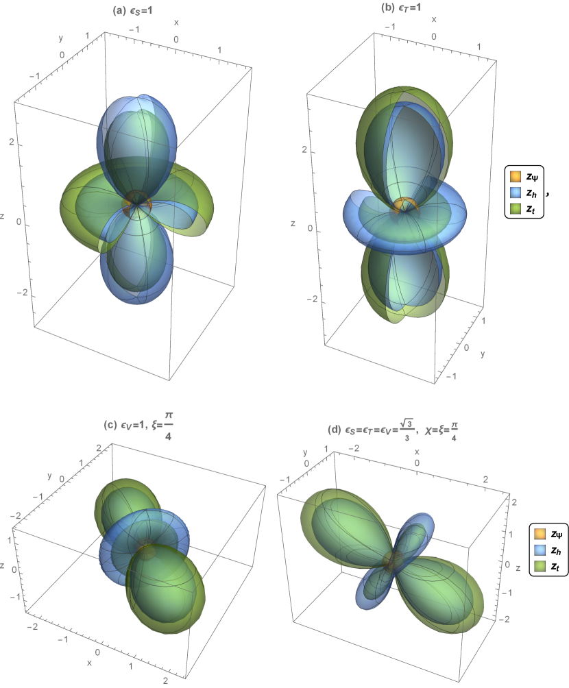
Figure 1: The redshift induced by the tensor ULDM under four different cases: (a) only the scalar mode exists: $\epsilon_{\rm{S}}=1,\epsilon_{\rm{T}}=\epsilon_{\rm{V}}=0$; (b) only the tensor modes exist: $\epsilon_{\rm{T}}=1,\epsilon_{\rm{S}}=\epsilon_{\rm{V}}=0$; (c) only the vector modes exist: $\epsilon_{\rm{V}}=1,\epsilon_{\rm{S}}=\epsilon_{\rm{T}}=0$; (d) all five polarization modes exist with the specific values: $\epsilon_{\rm{V}}=\epsilon_{\rm{S}}=\epsilon_{\rm{T}}=\frac{\sqrt{3}}{3}$ and $\chi=\xi=\frac{\pi}{4}$. The orange surface and blue surface represent the contribution of the trace part Eq. (42) and the traceless part Eq. (43), respectively; their summation, the total redshift Eq. (44), is depicted by the green surface.

As reported in Kolb et al. (2023), similar to the situation for spin-1 fields as discussed in Graham et al. (2016), the longitudinal scalar mode of the massive spin-2 field is more abundantly generated than the longitudinal-transverse vector and transverse tensor polarization modes. Here and after, we restrict ourselves to the scalar mode of the tensor ULDM, namely case a) in Fig. 1 where $\epsilon_{\rm{S}}=1,\epsilon_{\rm{T}}=\epsilon_{\rm{V}}=0$. To highlight the physical implications behind this case, we will explicitly derive the timing residual induced by the scalar sector below. The corresponding equation of motion can be written as

$$\begin{gathered}M_{ij}=\frac{1}{\sqrt{6}}A(\mathbf{x})\cos(mt+\alpha(\mathbf{x}))\begin{pmatrix}-1&0&0\\ 0&-1&0\\ 0&0&2\end{pmatrix},\end{gathered}$$ (47)

and the nonvanishing energy-momentum components are

$$T_{00} = \frac{1}{8}m^{2}A(\mathbf{x})^{2},$$ (48)

$$T_{xx} = T_{yy}=-\frac{1}{24}m^{2}A(\mathbf{x})^{2}\cos(2mt+2\alpha(\mathbf{x})),$$ (49)

$$T_{zz} = \frac{5}{24}m^{2}A(\mathbf{x})^{2}\cos(2mt+2\alpha(\mathbf{x})).$$ (50)

In this case, the metric perturbations $\Psi(\mathbf{x})$ and $h_{ij}(\mathbf{x})$ induced by the trace and traceless parts of the energy-momentum can be expressed as

$$\Psi(\mathbf{x}) =\Psi_{0}+\frac{1}{24}\pi GA(\mathbf{x})^{2}\cos(2mt+2\alpha(\mathbf{x})),$$

$$h_{ij}(\mathbf{x}) =\frac{1}{3}\pi GA(\mathbf{x})^{2}\cos(2mt+2\alpha(\mathbf{x}))\begin{pmatrix}1&0&0\\ 0&1&0\\ 0&0&-2\end{pmatrix}.$$ (51)

These perturbations lead to redshifts $z_{\Psi}$ (Eq. (42)) and $z_{h}$ (Eq. (43)) in the pulsar timing signal, which add up to yield the total redshift

$$z_{t} = z_{\Psi}+z_{h}$$ (52)

$$= -\frac{\pi G\rho_{\rm{TF}}}{3m^{2}}(1+6\cos 2\theta)\times\left[\cos(2mt+2\alpha(\mathbf{x}_{e}))-\cos\left(2m(t-|\mathbf{x}_{p}|)+2\alpha(\mathbf{x}_{p})\right)\right].$$

Integrating the redshift results in the final timing residual,

$$R_{t}=-\frac{\pi G\rho_{\rm{TF}}}{3m^{3}}(1+6\cos 2\theta)\sin(\alpha_{e}-\alpha_{p})\cos\left(2mt+\alpha_{e}+\alpha_{p}\right).$$ (53)

The above expression can also be derived by simply plugging the conditions $\epsilon_{\rm{S}}=1$ and $\epsilon_{\rm{T}}=\epsilon_{\rm{V}}=0$ into Eq. (45).

Recall that the coherent oscillations of scalar and vector ULDM also generate timing residuals (Khmelnitsky and Rubakov, 2014; Nomura et al., 2020),

$$R_{\rm{scalar}} = \frac{\pi G\rho_{\rm{SF}}}{m^{3}}\sin(\alpha_{e}-\alpha_{p})\cos\left(2mt+\alpha_{e}+\alpha_{p}\right),$$ (54)

$$R_{\rm{vector}} = -\frac{\pi G\rho_{\rm{VF}}}{m^{3}}(1+2\cos 2\theta)\sin(\alpha_{e}-\alpha_{p})\cos\left(2mt+\alpha_{e}+\alpha_{p}\right),$$ (55)

where $\rho_{\rm{SF}}$ and $\rho_{\rm{VF}}$ denote the energy density of the scalar fields and vector fields, respectively. As illustrated in Fig. 2, the amplitude and angular dependence of the signals induced by ULDM of different spins differ significantly. Notably, the timing residuals of scalar ULDM are isotropic, while those of vector ULDM and tensor ULDM exhibit nontrivial direction dependence.

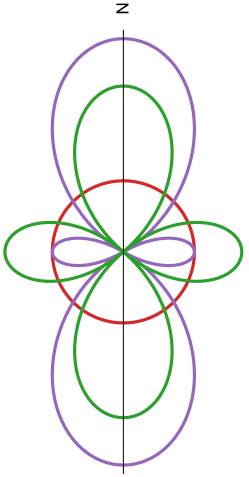
Figure 2: The redshift induced by oscillating ULDM with different spins. The red, purple and green lines represent the cases of the scalar, vector and tensor ULDM, respectively. The direction of oscillation is chosen along the z-axis for the vector and tensor ULDM.

IV Estimating the limits with current PTA

Several PTA data sets have been utilized to search for the scalar or the vector ULDM (Kato and Soda, 2020; Porayko et al., 2018; Wu et al., 2022). To make an approximate prediction of the tensor ULDM using the existing results, we take the average of Eq. (45) over the celestial sphere $\hat{p}$, which gives

$$\bar{R}_{t}=\sqrt{\frac{23}{15}}\frac{\pi G\rho_{\rm{TF}}}{m^{3}}\times\sin(\alpha_{e}-\alpha_{p})\cos\left(2mt+\alpha_{e}+\alpha_{p}\right).$$ (56)

Because of the system’s symmetry, the average timing residuals from the gravitational effect do not depend on the five parameters describing the quadruple but only on the energy density of the tensor ULDM $\rho_{\rm{TF}}$. To utilize previous results and facilitate later discussion, we replace $\rho_{\rm{TF}}$ with the unique quantity $h_{\rm{osc}}$ from the gravitational effect that is directly constrained by PTA experiments. Using the relationship Eq. (39), we obtain

$$\bar{R}_{t}=\frac{3}{4}\sqrt{\frac{23}{15}}\frac{h_{\rm{osc}}}{m}\times\sin(\alpha_{e}-\alpha_{p})\cos\left(2mt+\alpha_{e}+\alpha_{p}\right).$$ (57)

In Fig. 3, we present the constraint on the amplitude $h_{\rm{osc}}$ for tensor ULDM, which is reproduced from the bounds on the vector ULDM by the second dataset release of the Parkes PTA collaboration (PPTA DR2) (Wu et al., 2022).

Moreover, the spin-2 massive fields are universally coupled to the SM matter as a requirement of self-consistency of the model, which would cause a time delay for a pulse signal. The timing residual from the coupling effect is given by (Armaleo et al., 2020b),

$$\bar{R}_{c}=\sqrt{\frac{1}{15}}\frac{2\alpha\sqrt{\rho_{\rm{TF}}}}{m^{2}M_{\rm{P}}}\times\sin(\frac{\alpha_{e}-\alpha_{p}}{2})\cos\left(mt+\frac{\alpha_{e}+\alpha_{p}}{2}\right),$$ (58)

which depends on both the coupling $\alpha$ and the energy density $\rho_{\rm{TF}}$. Note that the timing residuals induced by the coupling effect, $\bar{R}_{c}$, and the gravitational effect, $\bar{R}_{t}$, have frequencies of $m$ and $2m$, respectively. If the spin-2 fields with a certain mass $m$ make up a significant fraction of the dark matter and the two effects are comparable, we will observe two signals in the PTA frequency band, with one having a frequency that is twice that of the other. Theoretically, it is difficult to determine the values of the two quantities $\alpha$ and $\rho_{\rm{TF}}$ from the coupling effect, as they are degenerate. However, we can first use the pure gravitational effect, given by Eq. (56), which depends solely on $\rho_{\rm{TF}}$, to determine whether massive spin-2 fields make up all dark matter. If we cannot exclude this possibility, we can estimate an upper bound for $\alpha$ using Eq. (57) and Eq. (58),

$$\alpha<\frac{3\sqrt{23}}{2}\frac{M_{\rm{P}}}{\sqrt{\rho_{\rm{0}}}}mh_{\rm{osc}},$$ (59)

where $\rho_{0}=0.4\rm{GeV/cm^{3}}$ is the measured local energy density (Salucci et al., 2010). If the spin-2 fields cannot make up all the dark matter, we need to estimate $\alpha$ using the $\rho_{\rm{TF}}$ obtained from the gravitational effect. In Fig. 3, we demonstrate several cases with different values of the coupling $\alpha$. We estimate that the coupling could get constrained at the level of $10^{-6}\sim 10^{-5}$ in the mass range $m<5\times 10^{-23}\rm{eV}$ with current PTA data.

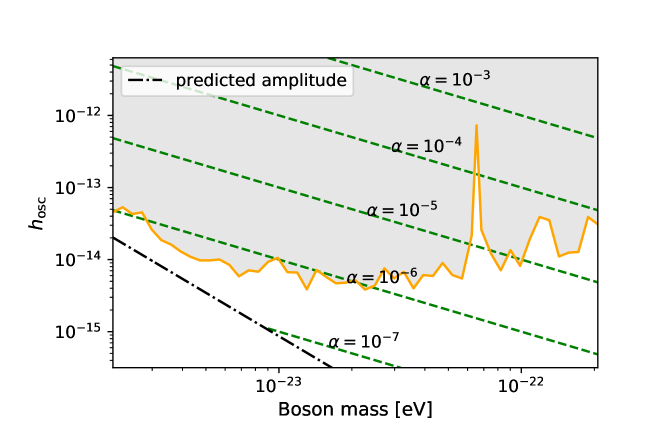
Figure 3: PPTA bounds on the potential amplitude $h_{\rm{osc}}$ induced by tensor ULDM versus the ULDM mass $m$. The black dot-dashed line denotes the model amplitude $h_{\rm{osc}}$ when assuming $\rho_{\rm{TF}}=0.4\rm{GeV/cm^{3}}$. The green dashed line represents the deductive coupling effect from $h_{\rm{osc}}$ for several values of the ULDM coupling $\alpha$.

V conclusion

In this work, we explore the gravitational effect of tensor ULDM on pulsar timing residuals. As a form of energy, the oscillating tensor field perturbs the spacetime geometry, resulting in the timing residuals that take the form of a sine function with a frequency equal to twice the particle mass, as shown in Eq. (45). Although the timing residuals of tensor ULDM depend on all five parameters describing the spin-2 quadrupole, it is pointed by (Kolb et al., 2023) that the gravitationally-produced massive spin-2 particles are predominantly longitudinally polarized, leading to a simpler expression Eq. (53) that still retains anisotropies. We find that the pulsar timing signal induced by the tensor ULDM exhibits a different angular dependence than that by the scalar and vector ULDM, as shown in Fig. 2.

Besides the gravitational effect, the coupling between the tensor ULDM and SM matter also produces sine-shaped timing residuals, depending both on the coupling $\alpha$ and the energy density of tensor fields $\rho_{\rm{TF}}$. In previous studies, the upper bound of $\alpha$ was estimated by assuming that the tensor ULDM constitutes all dark matter, which is reasonable since the current sensitivity is insufficient to exclude the assumption. However, as experimental precision continues to improve, it may become possible to use the gravitational effects to determine whether massive spin-2 fields can account for all dark matter. In such cases, it would be necessary to re-evaluate the coupling parameter using an updated energy density of the tensor ULDM. We present an estimation using this approach with PPTA DR2 in Fig. 3.

The timing residuals induced by scalar ULDM, vector ULDM, and tensor ULDM, as well as those induced by continuous gravitational waves emitted by a single supermassive black hole binary Zhu et al. (2014), exhibit distinct angular dependence. Therefore, the angular pattern of timing residuals can be used to distinguish different sources with PTA. However, just as disentangling multiple astrophysical and cosmological stochastic gravitational wave backgrounds is challenging (Kaiser et al., 2022), it may also be difficult to differentiate these monochromatic signals from each other. Therefore, investigating how they can be distinguished is an interesting research topic. In addition to the angular dependence, the correlation pattern of the timing residuals can be another tool to resolve different sources (Unal et al., 2022).