On the Decoherence of Primordial Gravitons

Abstract

It is well-known that the primordial scalar curvature and tensor perturbations, $\zeta$ and $\gamma_{ij}$, are conserved on super-horizon scales in minimal inflation models. However, their wave functional has a rapidly oscillating phase which is slow-roll unsuppressed, as can be seen either from boundary (total-derivative) terms of cosmological perturbations, or the WKB approximation of the Wheeler-DeWitt equation. Such an oscillatory phase involves gravitational non-linearity between scalar and tensor perturbations. By tracing out unobserved modes, the oscillatory phase causes faster decoherence of primordial gravitons compared to those by bulk interactions. Our results put a stronger lower bound of decoherence effect to the recent proposals probing squeezed primordial gravitons.

I Introduction

During inflation, the vacuum of the graviton evolves into a quantum squeezed state [1, 2, 3, 4], opening up possibilities to probe the non-classicality of gravitons via observations. There have been proposals to test the non-classicality of squeezed gravitons, including the quantum noise in gravitational-wave detectors and geodesics [5, 6, 7, 8, 9, 10, 11, 12], indirect detection through decoherence of matter [8, 17] and electromagnetic field [18], the Hanbury Brown-Twiss interferometry with the related sub-Poissonian statistics [19, 20, 21] and the interaction with an optical cavity [22, 23]. In particular, the quantum noise produced by the primordial gravitational wave can be largely enhanced by the inflationary squeezed states, providing a chance to make the non-classicality of gravitons detectable. However, it is well-known that the cosmological perturbations, including scalar and tensor, can experience the quantum-to-classical transition through the interaction with environment during inflation, described by the environment-induced decoherence. As a first step to analyze the potential obstruction of the mentioned proposals, we study the decoherence of the primordial gravitons during the simplest single-field inflation.

The environment-induced decoherence of scalar perturbations has been widely studied with various interactions and tools [24, 25, 26, 27, 28, 29, 30, 31, 32, 33, 34, 35, 36, 37, 38, 39, 40, 41, 42, 43], and some of the frameworks are also applicable to the decoherence of tensor perturbations. For the primordial gravitons, the possible sources of decoherence include the non-linear interaction between tensor modes [44], the scalar-tensor interaction [45, 38], and the primordial magnetic field [46, 47]. Focusing on the simplest single-field inflation, the decoherence effects of gravitons by scalar and tensor environments through the bulk interactions are comparable, and the quantum-to-classical transition happens at 7-9 e-folds after crossing the Hubble horizon, proving the upper bound of the purity of the primordial squeezed gravitons.

As noted recently in [41], the slow-roll unsuppressed boundary (total-derivative) term

$$\mathcal{L}_{{\rm bd},\zeta}=M_{p}^{2}\frac{d}{dt}\left(-2a^{3}He^{3\zeta}\right)\ ,$$ (1)

which dominates for the super-horizon scalar curvature perturbation $\zeta$, can introduce rapidly oscillating non-Gaussian phase to the wave functional of cosmological perturbations, leading to much larger decoherence than the bulk interactions. Such boundary terms without any time derivative $\dot{\zeta}$ (similarly for tensor perturbation $\dot{\gamma}_{ij}$) cannot contribute to correlators $\langle\zeta^{m}\gamma^{n}\rangle$, so they are often neglected in the literature, whereas they also cannot be removed by field redefinitions [48, 49, 50]. In this paper, we extend the boundary-term decoherence to the case with tensor perturbation, which relies on the slow-roll unsuppressed scalar-tensor cubic boundary terms

$$\mathcal{L}_{{\rm bd},\zeta-\gamma} =M_{p}^{2}\frac{d}{dt}\left[-\frac{a\partial_{i}\zeta\partial_{j}\zeta\gamma{}_{i}{}_{j}}{H}-\frac{a\zeta\left(\partial_{l}\gamma{}_{i}{}_{j}\right)^{2}}{8H}\right]\ ,$$ (2)

and we will show that these boundary terms also lead to larger decoherence than the bulk terms.

There is a constant interest in discussing the Wheeler-DeWitt (WDW) equation [51, 52] and quantum gravity [53, 54, 55, 56, 57], which motivates us to discuss the relationship between these boundary terms and the wave functional obtained by the WDW equation. In the large volume limit of inflation [58, 59, 60] and dS space [61, 62, 63, 64] or similarly the asymptotic infinity in AdS [65, 66, 54], the wave functional shares the same form, consisting of a real local action $W(h_{ij},\phi)$ and a part $Z(h_{ij},\phi)$ including non-local terms

$$\Psi(h_{ij},\phi) =e^{iW(h_{ij},\phi)}Z(h_{ij},\phi)\ ,$$ (3)

where $h_{ij}$ is the spatial metric induced on a hypersurface, and $\phi$ is the inflaton in our case. With the form of the wave functional (3), it is clear that the rapidly oscillating phase $W(h_{ij},\phi)$ cannot contribute to the expectation value of any observable defined by the spatial metric

$$\langle O(h_{ij})\rangle =\int Dh_{ij}\left|\Psi(h_{ij},\phi)\right|^{2}O(h_{ij})$$

$$=\int Dh_{ij}\left|Z(h_{ij},\phi)\right|^{2}O(h_{ij})\ ,$$ (4)

where we assume that $\Psi(h_{ij},\phi)$ is normalized and defined on the hypersurface with $\delta\phi=0$ (the $\zeta$-gauge), so all the quantum degrees of freedom are in the metric. The local action (or WKB phase) $W(h_{ij},\phi)$ can be calculated by applying the WKB approximation to the WDW equation [58, 59, 60], and we will show that it matches the non-Gaussian phase obtained from the boundary terms in the action of cosmological perturbations, thus contributing to the decoherence. It is noteworthy that the slow-roll suppressed scalar bulk interaction $\epsilon(\epsilon+\eta)a\left(\partial_{i}\zeta\right)^{2}\zeta$ studied in [34] also contributes a rapidly oscillating non-Gaussian phase at late time, thus the state is considered as the WKB type by the author, causing decoherence of $\zeta$ by tracing out unobserved modes. However, we will show that the WKB phase in the WDW state includes slow-roll unsuppressed parts involving both scalar $\zeta$ and tensor perturbations $\gamma_{ij}$.

The paper is organized as follows. In Sec. II, we review the setup of the simplest single-field inflation with a brief discussion of the choice of tensor perturbation and re-derive the splitting of bulk and boundary cubic terms. In Sec. III, we first discuss the non-Gaussian phase obtained from the slow-roll unsuppressed boundary terms in both the interaction and Schrödinger pictures, and we then check that it is consistent with the local phase obtained by solving the WDW equation with the WKB approximation. In Sec. IV, we calculate the decoherence effect of primordial gravitons by tracing out the unobserved scalar or tensor environments, confirming that the decoherence happens faster than the one caused by the bulk interactions. In Sec. V, we comment the one-loop quantum correction to the wave functional, including the contribution from the Faddeev-Popov ghost by diffeomorphism, and we argue that the correction is negligible in the leading decoherence effect. Sec. VI is the conclusion.

We set some notations for convenience. We label the comoving momenta of system modes with $\bf q$ and environment modes with $\bf k$, and the comoving momentum $\bf p$ can be used to label arbitrary modes. The integral modes with momentum conservation is denoted by $\int_{{\bf{p}}_{1},\cdots,{\bf{p}}_{n}}=\int\frac{d^{3}p_{1}}{(2\pi)^{3}}\cdots\frac{d^{3}p_{n}}{(2\pi)^{3}}(2\pi)^{3}\delta^{3}({\bf p}_{1}+\cdots+{\bf p}_{n})$, and integrating over two environment modes with a fixed system mode is $\int_{\bf{k}+\bf{k}^{\prime}=-\bf{q}}=\int\frac{d^{3}k}{(2\pi)^{3}}\frac{d^{3}k^{\prime}}{(2\pi)^{3}}(2\pi)^{3}\delta^{3}(\bf{k}+\bf{k}^{\prime}+\bf{q})$. We use a simpler notation $\sum_{s_{1},\cdots,s_{n}}=\sum_{s_{1},\cdots,s_{n}=+,-}$ to represent the sum of $n$ circular polarization indices.

II The bulk and boundary terms in the cubic order

In this section, we review the setup for deriving the action of cosmological perturbations up to the cubic order [67] with a brief comment on the two common choices of tensor perturbation in the literature. Since the neglected temporal boundary terms obtained by integration by parts are not clearly shown in [67], we also derive the splitting of bulk and boundary terms for both scalar and tensor perturbations.

II.1 The setup

We start with the ADM decomposition of the metric

$$ds^{2}=-N^{2}dt^{2}+h_{ij}\left(dx^{i}+N^{i}dt\right)\left(dx^{j}+N^{j}dt\right)\ ,$$ (5)

where $N$ and $N^{i}$ are the lapse and shift respectively, and $h_{ij}$ is the spatial metric on the hypersurface which has the extrinsic curvature

$$K_{\mu\nu}=\left(\delta^{\rho}_{\mu}+n^{\rho}n_{\mu}\right)\nabla_{\rho}n_{\nu}\ ,$$ (6)

where $n^{\mu}$ is the normal of the hypersurface. We consider the simplest single-field inflation with the action

$$S =\int_{\mathcal{M}}d^{4}x\sqrt{-g}\left[\frac{M_{p}^{2}}{2}R-\frac{1}{2}g^{\mu\nu}\partial_{\mu}\phi\partial_{\nu}\phi-V(\phi)\right]-\int_{\partial\mathcal{M}}d^{3}xM_{p}^{2}\sqrt{h}K$$

$$=\frac{M_{p}^{2}}{2}\int_{\mathcal{M}}d^{4}x\sqrt{h}\left[N\left({{}^{(3)}}R-K^{2}+K_{ij}K^{ij}\right)+\frac{1}{N}\left(\dot{\phi}-N^{i}\partial_{i}\phi\right)^{2}-Nh^{ij}\partial_{i}\phi\partial_{j}\phi-2NV(\phi)\right]\ .$$ (7)

where the second term in the first line is the Gibbons-Hawking-York (GHY) boundary term for the manifold $\mathcal{M}$ [68, 69, 70] which cancels with the covariant derivative term when we decompose the 4-dimensional Ricci scalar

$$R ={{}^{(3)}R}-K^{2}+K^{\mu}_{\nu}K^{\nu}_{\mu}-2\nabla_{\mu}\left(-Kn^{\mu}+n^{\nu}\nabla_{\nu}n^{\mu}\right)\ ,$$ (8)

with ${{}^{(3)}R}$ the three-dimensional Ricci scalar. The Hubble parameter is determined by the uniform background of inflaton field as

$$3M_{p}^{2}H^{2} =\frac{1}{2}\dot{\phi}^{2}+V(\phi)\ ,$$ (9)

with which the slow-roll parameters are defined

$$\epsilon=-\frac{\dot{H}}{H^{2}}\ ,\ \eta=\frac{\dot{\epsilon}}{H\epsilon}\ ,$$ (10)

satisfying the slow-roll conditions $\epsilon\ll 1$ and $|\eta|\ll 1$.

In the literature, there are two definitions of tensor perturbations in the spatial metric $h_{ij}$ which are applied in the decoherence problems [44, 45], and here we briefly discuss the difference. One is $\gamma_{ij}$ defined in the comoving gauge ($\zeta$-gauge with $\delta\phi=0$), e.g. in [67]

$$h_{ij} =a^{2}e^{2\zeta}(e^{\gamma})_{ij}\ ,$$ (11)

where $\zeta$ is the scalar curvature perturbation, and $\gamma_{ij}$ satisfies $\gamma_{ii}=\partial_{i}{\gamma_{ij}}=0$. Another is defined by the scalar-vector-tensor decomposition [71]

$$h_{ij} =a^{2}\left(\delta_{ij}+\frac{h_{S}}{3}\delta_{ij}+h^{TT}_{ij}\right)\ ,$$ (12)

which includes the scalar part $h_{S}$ and the transverse traceless part $h^{TT}_{ij}$. The curvature perturbation $\zeta$ is related to $(h_{S},h^{TT}_{ij})$ on the hypersurface with $\delta\phi=0$ by comparing the same $\det(h_{ij})$ calculated in (11) and (12)

$$\zeta\left(h_{S},h^{TT}_{ij}\right) \approx\frac{h_{S}}{6}-\frac{1}{36}\left(h_{S}^{2}+3h^{TT}_{ij}h^{TT}_{ij}\right)+\mathcal{O}\left(h_{S}^{3},\left(h_{ij}^{TT}\right)^{3}\right)\ ,$$ (13)

showing the dependence between $\zeta$ and $h_{ij}^{TT}$, so $h_{ij}^{TT}$ may not be a good choice when $\zeta$ is considered as the environment of decoherence of gravitons. Therefore, under the condition $\delta\phi=0$, one may either choose $(\zeta,\gamma_{ij})$ or $(h_{S},h^{TT}_{ij})$ to be the scalar and tensor perturbations to make the calculation convenient and avoid some ambiguities.

On the other hand, $\gamma_{ij}$ defined in the first case conserves outside the horizon, as the cubic interactions related to $\gamma_{ij}$ all include derivatives which will be shown explicitly in (27)-(29). However, $h^{TT}_{ij}$ does not conserve outside the horizon as the cubic interactions include a term without any derivative [44]

$$\mathcal{L}_{h^{TT}h^{TT}h^{TT}}\supset 2\left(1-\frac{\epsilon}{3}\right)M_{p}^{2}H^{2}a^{3}h^{TT}_{ij}h^{TT}_{jl}h^{TT}_{li}\ ,$$ (14)

suggesting that $\gamma_{ij}$ is more convenient to the describe the super-horizon evolution of tensor mode. As also discussed in [72], gravitational wave should not perturb the spatial volume, and the property $\det(e^{\gamma})_{ij}=1$ also suggests that $\gamma_{ij}$ is more appropriate.

Due to the mentioned reasons, we adopt the spatial metric defined with $\left(\zeta,\gamma_{ij}\right)$ (11), consistent with the choice in [34, 41, 45]. Varying the action (7) with respect to $N$ and $N^{i}$ gives the constraint equations, solving them gives

$$N=1+\frac{\dot{\zeta}}{H}\ ,\ N^{i}=\frac{1}{a^{2}}\left(-\frac{\partial_{i}\zeta}{H}+\partial_{i}\chi\right)\ ,\ \partial^{2}\chi=a^{2}\epsilon\dot{\zeta}\ .$$ (15)

With these, expanding the action (7) to the second order gives the free actions of scalar

$$S^{(\zeta)}_{2} =M_{p}^{2}\int dtd^{3}x\ \epsilon a^{3}\left[\dot{\zeta}^{2}-a^{-2}\left(\partial_{i}\zeta\right)^{2}\right]$$

$$=M_{p}^{2}\int dt\frac{d^{3}p}{(2\pi)^{3}}\ \epsilon a^{3}\left(\dot{\zeta}_{\bf p}\dot{\zeta}_{-{\bf p}}-\frac{p^{2}}{a^{2}}\zeta_{\bf p}\zeta_{-{\bf p}}\right)\ ,$$ (16)

and tensor perturbations

$$S^{(\gamma)}_{2} =\frac{M_{p}^{2}}{8}\int dtd^{3}x\ a^{3}\left[\dot{\gamma}_{ij}\dot{\gamma}_{ij}-a^{-2}\left(\partial_{l}\gamma_{ij}\right)^{2}\right]$$

$$=\frac{M_{p}^{2}}{2}\sum_{s}\int dt\frac{d^{3}p}{(2\pi)^{3}}\ a^{3}\left(\dot{\gamma}^{s}_{\bf p}\dot{\gamma}^{s}_{-{\bf p}}-\frac{p^{2}}{a^{2}}\gamma^{s}_{\bf p}\gamma^{s}_{-{\bf p}}\right)\ ,$$ (17)

where in the second line the following mode decomposition is applied [73]

$$\gamma_{ij}({\bf x},t)=\sum_{s}\int\frac{d^{3}p}{(2\pi)^{3}}\gamma^{s}_{\bf p}(t)e^{s}_{ij}({\bf p})e^{i{\bf p}\cdot{\bf x}}\ ,$$ (18)

and the symmetric polarization tensors satisfy

$$e^{\pm}_{ij}(-{\bf p}) =\left(e^{\pm}_{ij}({\bf p})\right)^{*}$$

$$e^{s}_{ij}({\bf p})(e^{s^{\prime}}_{ij}({\bf p}))^{*} =4\delta_{s,s^{\prime}}$$

$$e^{\pm}_{ii}({\bf p}) =0$$

$$p_{i}e^{\pm}_{ij}({\bf p}) =0\ .$$ (19)

By quantizing $\zeta$ and $\gamma_{ij}$, the free actions (16) and (17) imply a time-dependent Gaussian wave functional [67]

$$\Psi_{G}(\zeta,\gamma) =N_{G}(\tau)\exp\left(-\frac{1}{2}\int\frac{d^{3}p}{(2\pi)^{3}}A^{(\zeta)}_{p}(\tau)\zeta_{\bf p}\zeta_{-{\bf p}}-\frac{1}{2}\sum_{s}\int\frac{d^{3}p}{(2\pi)^{3}}A^{(\gamma)}_{p}(\tau)\gamma^{s}_{\bf p}\gamma^{s}_{-{\bf p}}\right)\ ,$$ (20)

where the normalization factor $N_{G}=\prod_{\bf p}N_{G,{\bf p}}^{(\zeta)}N_{G,{\bf p}}^{(\gamma)}$ is separable, and the coefficients

$$A^{(\zeta)}_{p}(\tau) =-2\epsilon M_{p}^{2}\frac{i}{(H\tau)^{2}}\frac{{u^{\prime}}^{(\zeta)}_{p}(\tau)}{u^{(\zeta)}_{p}(\tau)}$$

$$=2p^{3}\frac{\epsilon M_{p}^{2}}{H^{2}}\frac{1-\frac{i}{p\tau}}{1+p^{2}\tau^{2}}\ ,$$ (21)

$$A^{(\gamma)}_{p}(\tau) =-M_{p}^{2}\frac{i}{(H\tau)^{2}}\frac{{u^{\prime}}^{(\gamma)}_{p}(\tau)}{{u}^{(\gamma)}_{p}(\tau)}$$

$$=p^{3}\frac{M_{p}^{2}}{H^{2}}\frac{1-\frac{i}{p\tau}}{1+p^{2}\tau^{2}}\ ,$$ (22)

where $\tau=\int^{t}\frac{dt^{\prime}}{a(t^{\prime})}$ is the conformal time with ${}^{\prime}=\frac{d}{d\tau}$, and the mode functions are

$$u^{(\zeta)}_{p}(\tau) =\frac{H}{2M_{p}\sqrt{\epsilon p^{3}}}(1-ip\tau)e^{ip\tau}$$

$$u^{(\gamma)}_{p}(\tau) =\frac{H}{M_{p}\sqrt{2p^{3}}}(1-ip\tau)e^{ip\tau}.$$ (23)

For the Gaussian wave functional (20), the scalar and tensor power spectra are related to the two coefficients (21) and (22) as

$$P^{(\zeta,\gamma)}_{p}(\tau) =\frac{1}{2{\rm Re}A^{(\zeta,\gamma)}_{p}(\tau)}\ .$$ (24)

At the quadratic level, all the modes evolve independently, and thus we need the cubic order action for the interactions between observed and unobserved modes.

II.2 Splitting the bulk and boundary cubic terms

We want to find out all the scalar and tensor temporal boundary terms neglected in [67], as they will be shown to be important to the inflationary decoherence. The guideline of splitting the bulk and boundary terms in the $\zeta$-gauge is to make the former matches the one derived in the $\delta\phi$-gauge (spatially flat) (see also [74, 75, 50] by arranging the bulk terms in the gauge-invariant manner), and it is expected that all the cubic bulk terms involving $\zeta$ is slow-roll suppressed since the transformation $\delta\phi\approx-\frac{\dot{\phi}}{H}\zeta\sim\mathcal{O}(\sqrt{\epsilon})\zeta$ introduces slow-roll parameters. On the other hand, since the tensor perturbations in the two gauges are on the same slow-roll order, bulk terms include some slow-roll unsuppressed $\gamma\gamma\gamma$ interactions.

The splitting of the bulk and boundary interactions can be found in the literature [49, 76, 50], and here we derive again with the notations used in this paper. With the Mathematica package MathGR [77] doing integration by parts, we obtain the following splitting of bulk and boundary cubic terms from the action (7) (with spatial total derivative neglected)

$$\mathcal{L}^{(3)}=\mathcal{L}_{\zeta\zeta\zeta}+\mathcal{L}_{\zeta\zeta\gamma}+\mathcal{L}_{\zeta\gamma\gamma}+\mathcal{L}_{\gamma\gamma\gamma}+f(\zeta,\gamma)\frac{\delta L_{2}}{\delta\zeta}+f_{ij}(\zeta,\gamma)\frac{\delta L_{2}}{\delta\gamma_{ij}}+\mathcal{L}_{\rm bd,\zeta\zeta\zeta}+\mathcal{L}_{\rm bd,\zeta\zeta\gamma}+\mathcal{L}_{\rm bd,\zeta\gamma\gamma}\ ,$$ (25)

where the four bulk terms

$$\mathcal{L}_{\zeta\zeta\zeta} =M_{p}^{2}\left[a^{3}\epsilon(\epsilon-\eta)\zeta\dot{\zeta}^{2}+a\epsilon(\epsilon+\eta)\zeta(\partial_{i}\zeta)^{2}+\left(\frac{\epsilon}{2}-2\right)\frac{\partial^{2}\chi}{a}\partial_{i}\chi\partial_{i}\zeta+\frac{\epsilon}{4a}\partial^{2}\zeta\left(\partial_{i}\chi\right)^{2}\right]$$ (26)

$$\mathcal{L}_{\zeta\zeta\gamma} =M_{p}^{2}\left[-\frac{1}{2}a\epsilon\chi\partial_{i}\partial_{j}\zeta\dot{\gamma}_{i}{}_{j}+\frac{\partial_{i}\chi\partial_{j}\chi\partial^{2}\gamma_{i}{}_{j}}{4a}+a\epsilon\partial_{i}\zeta\partial_{j}\zeta\gamma_{i}{}_{j}\right]$$ (27)

$$\mathcal{L}_{\zeta\gamma\gamma} =M_{p}^{2}\left[\frac{1}{8}a^{3}\epsilon\zeta\dot{\gamma}{}_{i}{}_{j}{}^{2}-\frac{1}{4}a\partial_{l}\chi\dot{\gamma}{}_{i}{}_{j}\partial_{l}\gamma{}_{i}{}_{j}+\frac{1}{8}a\epsilon\zeta\left(\partial_{l}\gamma{}_{i}{}_{j}\right)^{2}\right]$$ (28)

$$\mathcal{L}_{\gamma\gamma\gamma} =M_{p}^{2}\left[\frac{1}{4}a\partial_{m}\gamma{}_{i}{}_{l}\partial_{l}\gamma{}_{j}{}_{m}\gamma{}_{i}{}_{j}+\frac{1}{8}a\partial_{i}\gamma{}_{l}{}_{m}\partial_{j}\gamma{}_{l}{}_{m}\gamma{}_{i}{}_{j}\right]\ ,$$ (29)

the two EOM terms

$$f(\zeta,\gamma) =-\frac{\dot{\zeta}\zeta}{H}+\frac{1}{4a^{2}H^{2}}\left[\left(\partial_{i}\zeta\right)^{2}-\partial^{-2}\partial_{i}\partial_{j}\left(\partial_{i}\zeta\partial_{j}\zeta\right)\right]-\frac{1}{2a^{2}H}\left[\partial_{i}\zeta\partial_{i}\chi-\partial^{-2}\partial_{i}\partial_{j}\left(\partial_{i}\zeta\partial_{j}\chi\right)\right]$$

$$+\frac{\partial_{i}\partial_{j}\zeta\dot{\gamma}{}_{i}{}_{j}}{4H}\partial^{-2}$$ (30)

$$f_{ij}(\zeta,\gamma) =-\frac{\zeta\dot{\gamma}{}_{i}{}_{j}}{H}+\frac{\partial_{i}\zeta\partial_{j}\zeta}{a^{2}H^{2}}+\frac{2\chi\partial_{i}\partial_{j}\zeta}{a^{2}H}$$ (31)

$$\frac{\delta L_{2}}{\delta\zeta} =2M_{p}^{2}\left[-\frac{d}{dt}\left(\epsilon a^{3}\dot{\zeta}\right)+\epsilon a\partial^{2}\zeta\right]$$ (32)

$$\frac{\delta L_{2}}{\delta\gamma_{ij}} =\frac{M_{p}^{2}}{4}\left[-\frac{d}{dt}\left(a^{3}\dot{\gamma}_{ij}\right)+a\partial^{2}\gamma_{ij}\right]\ ,$$ (33)

and the boundary terms

$$\mathcal{L}_{\rm bd,\zeta\zeta\zeta} =M_{p}^{2}\frac{d}{dt}\Bigg{\{}-9a^{3}H\zeta^{3}+\frac{a}{H}\left(1-\epsilon\right)\zeta\left(\partial_{i}\zeta\right)^{2}-\frac{1}{4aH^{3}}\left(\partial_{i}\zeta\right)^{2}\partial^{2}\zeta$$

$$-\frac{\epsilon a^{3}}{H}\zeta\dot{\zeta}^{2}-\frac{\zeta}{2aH}\left[\left(\partial_{i}\partial_{j}\chi\right)^{2}-\left(\partial^{2}\chi\right)^{2}\right]+\frac{\zeta}{2aH^{2}}\left(\partial_{i}\partial_{j}\zeta\partial_{i}\partial_{j}\chi-\partial^{2}\zeta\partial^{2}\chi\right)\Bigg{\}}$$ (34)

$$\mathcal{L}_{\rm bd,\zeta\zeta\gamma} =M_{p}^{2}\frac{d}{dt}\left(-\frac{a\partial_{i}\zeta\partial_{j}\zeta\gamma{}_{i}{}_{j}}{H}+\frac{a\partial_{i}\zeta\partial_{j}\zeta\dot{\gamma}{}_{i}{}_{j}}{4H^{2}}+\frac{a\chi\partial_{i}\partial_{j}\zeta\dot{\gamma}{}_{i}{}_{j}}{2H}\right)$$ (35)

$$\mathcal{L}_{\rm bd,\zeta\gamma\gamma} =M_{p}^{2}\frac{d}{dt}\left[-\frac{a\zeta\left(\partial_{l}\gamma{}_{i}{}_{j}\right)^{2}}{8H}-\frac{a^{3}\zeta\dot{\gamma}{}_{i}{}_{j}{}^{2}}{8H}\right]\ .$$ (36)

Using the size of power spectra of scalar and tensor perturbations

$$\Delta^{2}_{\zeta} =\lim_{\tau\to 0}\frac{p^{3}}{2\pi^{2}}P^{(\zeta)}_{p}(\tau)=\frac{H^{2}}{8\pi^{2}\epsilon M_{p}^{2}}\ ,$$ (37)

$$\Delta^{2}_{\gamma} =\lim_{\tau\to 0}\frac{p^{3}}{2\pi^{2}}\sum_{s,s^{\prime}}P^{(\gamma)}_{p}(\tau)4\delta_{s,s^{\prime}}=\frac{2H^{2}}{\pi^{2}M_{p}^{2}}\ ,$$ (38)

we expect that the tensor perturbation is slow-roll suppressed compared to the scalar perturbation $\gamma\sim\mathcal{O}(\sqrt{\epsilon})\zeta$. Table 1 is the summary of the size of interaction terms which do not involve any time derivative, and only the most dominated terms of each type are shown. It is clear that boundary terms are less slow-roll suppressed compared to the bulk terms.

bulk/boundary	type	leading interaction of each type	order
bulk	$\zeta\zeta\zeta$	$\epsilon(\epsilon+\eta)a(\partial_{i}\zeta)^{2}\zeta$	$\epsilon(\epsilon+\eta)\zeta^{3}$
bulk	$\zeta\zeta\gamma$	$\epsilon a\partial_{i}\zeta\partial_{j}\zeta\gamma_{ij}$	$\epsilon^{\frac{3}{2}}\zeta^{3}$
bulk	$\zeta\gamma\gamma$	$\epsilon a\zeta\partial_{l}\gamma_{ij}\partial_{l}\gamma_{ij}$	$\epsilon^{2}\zeta^{3}$
bulk	$\gamma\gamma\gamma$	$a\partial_{i}\gamma{}_{l}{}_{m}\partial_{j}\gamma{}_{l}{}_{m}\gamma{}_{i}{}_{j}$	$\epsilon^{\frac{3}{2}}\zeta^{3}$
boundary	$\zeta\zeta\zeta$	$\partial_{t}(a^{3}\zeta^{3})$	$\zeta^{3}$
boundary	$\zeta\zeta\gamma$	$\partial_{t}(a\partial_{i}\zeta\partial_{j}\zeta\gamma_{ij})$	$\epsilon^{\frac{1}{2}}\zeta^{3}$
boundary	$\zeta\gamma\gamma$	$\partial_{t}(a\zeta\partial_{l}\gamma_{ij}\partial_{l}\gamma_{ij})$	$\epsilon\zeta^{3}$

Table 1: The leading interaction terms of each type and their orders of magnitudes.

III The oscillating phase of inflationary wave functional

It has been shown in the literature [48, 49, 76] that total time derivative terms in the Lagrangian $\mathcal{L}_{\rm int}\supset-\partial_{t}\mathcal{K}$ generally contribute to the in-in correlators as

$$\langle O(t)\rangle =\left\langle 0\left|\bar{T}\exp\left(i\int d^{3}x\int^{t}_{t_{i}}dt^{\prime}\ \partial_{t^{\prime}}\mathcal{K}\left(t^{\prime}\right)\right)O(t)T\exp\left(-i\int d^{3}x\int^{t}_{t_{i}}dt^{\prime}\ \partial_{t^{\prime}}\mathcal{K}\left(t^{\prime}\right)\right)\right|0\right\rangle$$

$$=\left\langle 0\left|\exp\left(i\int d^{3}x\ \mathcal{K}(t)\right)O(t)\exp\left(-i\int d^{3}x\ \mathcal{K}(t)\right)\right|0\right\rangle$$

$$\approx i\int d^{3}x\langle 0|\left[\mathcal{K}(t),O(t)\right]|0\rangle+\mathcal{O}(\mathcal{K}^{2})\ .$$ (39)

Since decoherence is mainly contributed by terms without time derivatives [45], we focus on the boundary terms involving $\zeta$, $\gamma_{ij}$ and their spatial derivatives, denoted by $\mathcal{K}\left(\zeta,\gamma,t\right)$ with the explicit forms shown in (34)-(36). $\mathcal{K}\left(\zeta,\gamma,t\right)$ commutes with normal correlators of the form $O(t)=\zeta^{m}(t)\gamma^{n}(t)$, and the expectation value in (39) vanishes, so such boundary terms are often neglected in the literature. In this section, we will show how such boundary terms contribute a non-Gaussian phase to the wavefunctional of cosmological perturbations with three methods. Sec. III.1 and III.2 calculate the phase with the interaction and Schrödinger pictures respectively, and the results will be shown to be consistent in (41) and (47). In Sec. III.3, we show that such a phase also matches the WKB approximation of the WDW equation, indicated by the WKB phase $W(h_{ij},\phi)$ in (3), and the explicit result will be shown in (59).

III.1 The interaction picture

It is straightforward to generalize the interaction picture approach in [41] to the case with tensor perturbation $\gamma_{ij}$, and the evolution operator is

$$U(\tau,\tau_{i}) =U_{0}(\tau,\tau_{i})T\exp\left(-i\int d^{3}x\int^{t}_{t_{i}}dt^{\prime}\ \partial_{t^{\prime}}\mathcal{K}\left(\zeta_{I},\gamma_{I},t^{\prime}\right)\right)$$

$$=U_{0}(\tau,\tau_{i})\sum_{n=0}^{\infty}\frac{(-i)^{n}}{n!}\left(\mathcal{K}(\zeta_{I},\gamma_{I},\tau)\right)^{n}$$

$$=\sum_{n=0}^{\infty}\frac{(-i)^{n}}{n!}\left(U_{0}(\tau,\tau_{i})\mathcal{K}(\zeta_{I},\gamma_{I},\tau)U^{-1}_{0}(\tau,\tau_{i})\right)^{n}U_{0}(\tau,\tau_{i})$$

$$=\exp\left(-i\int d^{3}x\ \mathcal{K}\left(\zeta_{S},\gamma_{S},\tau\right)\right)U_{0}(\tau,\tau_{i})\ ,$$ (40)

where $U_{0}(\tau,\tau_{i})=U^{(\zeta)}_{0}(\tau,\tau_{i})U^{(\gamma)}_{0}(\tau,\tau_{i})$ is the free evolution operator, and the labels $I$ and $S$ are the interaction and Schrödinger pictures respectively. Applying $U(\tau,\tau_{i})$ (40) to the initial Gaussian state $|\Psi_{G}(\tau_{i})\rangle$ gives a phase to the Schrödinger wave functional

$$\left\langle\zeta,\gamma|\Psi(\tau)\right\rangle=\exp\left(-i\int d^{3}x\ \mathcal{K}\left(\zeta,\gamma,\tau\right)\right)\Psi_{G}(\zeta,\gamma)\ .$$ (41)

III.2 The Schrödinger picture

We can also canonically quantize the theory with the boundary terms

$$\mathcal{L}=\mathcal{L}_{2}^{(\zeta)}+\mathcal{L}_{2}^{(\gamma)}-\partial_{t}\mathcal{K}\ ,$$ (42)

with

$$\mathcal{L}_{2}^{(\zeta)}+\mathcal{L}_{2}^{(\gamma)} =f_{aa}(t)\dot{\alpha}^{a}\dot{\alpha}^{a}+j_{aa}(t)\alpha^{a}\alpha^{a}\ ,$$

$$\mathcal{K}(\zeta,\gamma,t) =F_{abc}(t)\alpha^{a}\alpha^{b}\alpha^{c}\ ,$$ (43)

where we use a more compact notation $\vec{\alpha}=\alpha^{a}$ to denote the dynamic fields $\zeta$ and $\gamma_{ij}$ for making the derivation simpler and more generic, so $j_{aa}$ and $F_{abc}$ can include comoving momenta and polarization tensors expressed in the Fourier space. With these notations, the total time derivative has the form

$$\partial_{t}\mathcal{K}=\dot{F}_{abc}\alpha^{a}\alpha^{b}\alpha^{c}+F_{abc}\left(\dot{\alpha}^{a}\alpha^{b}\alpha^{c}+\alpha^{a}\dot{\alpha}^{b}\alpha^{c}+\alpha^{a}\alpha^{b}\dot{\alpha}^{c}\right)\ ,$$ (44)

and the conjugate momenta are defined as

$$\Pi_{a} =\frac{\partial\mathcal{L}}{\partial\dot{\alpha}^{a}}$$

$$=2f_{bb}\delta^{b}_{a}\dot{\alpha}^{b}-\left(F_{dbc}+F_{bdc}+F_{bcd}\right)\delta^{d}_{a}\alpha^{b}\alpha^{c}$$

$$=-i\frac{\delta}{\delta\alpha^{a}}\ ,$$ (45)

leading to the Hamiltonian density

$$\mathcal{H} =\dot{\alpha}^{a}\Pi_{a}-\mathcal{L}$$

$$=f_{aa}\dot{\alpha}^{a}\dot{\alpha}^{a}-j_{aa}\alpha^{a}\alpha^{a}+\dot{F}_{abc}\alpha^{a}\alpha^{b}\alpha^{c}$$

$$=\frac{1}{4f_{aa}}\left[-i\frac{\delta}{\delta\alpha^{a}}+\bar{F}_{abc}\alpha^{b}\alpha^{c}\right]\left[-i\frac{\delta}{\delta\alpha^{a}}+\bar{F}_{abc}\alpha^{b}\alpha^{c}\right]-j_{aa}\alpha^{a}\alpha^{a}+\dot{F}_{abc}\alpha^{a}\alpha^{b}\alpha^{c}\ ,$$ (46)

where $\bar{F}_{abc}=F_{abc}+F_{bac}+F_{bca}$. We can easily check that the wavefunctional with the non-Gaussian phase (41), rewritten with the compact notations

$$\Psi({\vec{\alpha}}) =N(t)e^{-\int\frac{A_{a}}{2}\alpha^{a}\alpha^{a}}e^{-i\int F_{abc}\alpha^{a}\alpha^{b}\alpha^{c}}\ ,$$ (47)

where $\int$ denotes integrals in the Fourier space, satisfies the Schrödinger equation

$$i\partial_{t}\Psi =\left(i\dot{N}-iN\int\frac{\dot{A}_{a}}{2}\alpha^{a}\alpha^{a}+N\int\dot{F}_{abc}\alpha^{a}\alpha^{b}\alpha^{c}\right)e^{-\int\frac{A_{a}}{2}\alpha^{a}\alpha^{a}}e^{-i\int F_{abc}\alpha^{a}\alpha^{b}\alpha^{c}}\ ,$$

$$\int\mathcal{H}\Psi =\left[\int\frac{A_{a}}{4f_{aa}}-\left(\frac{A^{2}_{a}}{4f_{aa}}+j_{aa}\right)\alpha^{a}\alpha^{a}+\int\dot{F}_{abc}\alpha^{a}\alpha^{b}\alpha^{c}\right]Ne^{-\int\frac{A_{a}}{2}\alpha^{a}\alpha^{a}}e^{-i\int F_{abc}\alpha^{a}\alpha^{b}\alpha^{c}}\ ,$$

$$i\partial_{t}\Psi =\int\mathcal{H}\Psi\ .$$ (48)

For the first two lines in (48), we applied the conditions obtained from the free theory (independent to $F_{abc}$) [32]

$$i\dot{N}=\int\frac{A_{a}}{4f_{aa}}N\ ,\quad i\frac{\dot{A}_{a}}{2}=\frac{A^{2}_{a}}{4f_{aa}}+j_{aa}\ ,$$ (49)

and the following relations

$$\left[-i\frac{\delta}{\delta\alpha^{a}}+\bar{F}_{abc}\alpha^{b}\alpha^{c}\right]\Psi({\vec{\alpha}}) =iA_{a}\alpha^{a}\Psi({\vec{\alpha}})\ ,$$

$$\left[-i\frac{\delta}{\delta\alpha^{a}}+\bar{F}_{abc}\alpha^{b}\alpha^{c}\right]^{2}\Psi({\vec{\alpha}}) =\left(A_{a}-A_{a}^{2}\alpha^{a}\alpha^{a}\right)\Psi({\vec{\alpha}})\ .$$ (50)

III.3 The WKB approximation of the Wheeler-DeWitt equation

The boundary terms can also be obtained by applying the WKB approximation to the wave function of universe $\Psi(h_{ij},\phi)$, obtained with the WDW equation [51, 52]. In [59, 60], the WDW equation of gravity with a scalar field has been applied to analyze the consistency relation and bispectrum, and we follow the formalism. We start with the Hamiltonian corresponding to the action (7), defined on the hypersurface $\Sigma$ inducing $h_{ij}$,

$$H =\int_{\Sigma}d^{3}x\Bigg{\{}N\left[\frac{1}{2\kappa\sqrt{h}}G_{ij,kl}\pi^{ij}\pi^{kl}-\kappa\sqrt{h}\ {{}^{(3)}}R+\frac{1}{4\kappa\sqrt{h}}\pi_{\phi}^{2}+\kappa\sqrt{h}\left(h^{ij}\partial_{i}\phi\partial_{j}\phi+2V(\phi)\right)\right]$$

$$+2\nabla_{i}N_{j}\pi^{ij}+h^{ij}N_{j}\partial_{i}\phi\pi_{\phi}\Bigg{\}}\ ,$$ (51)

where $\kappa=\frac{M_{p}^{2}}{2}$, the conjugate momenta are

$$\pi^{ij} =\frac{M_{p}^{2}}{2}\sqrt{h}\left(K^{ij}-h^{ij}K\right)$$

$$\pi_{\phi} =M_{p}^{2}\frac{\sqrt{h}}{N}\left(\dot{\phi}-N^{i}\partial_{i}\phi\right)\ ,$$ (52)

and the DeWitt metric is

$$G_{ij,kl}=h_{ik}h_{jl}+h_{il}h_{jk}-h_{ij}h_{kl}\ .$$ (53)

By promoting the conjugate momenta (52) to functional derivatives $\left(-i\hbar\frac{\delta}{\delta h_{ij}},-i\hbar\frac{\delta}{\delta\phi}\right)$ ($\hbar$ is restored for the moment) and varying (51) with respect to $\left(N,N_{i}\right)$, we obtain the Hamiltonian and momentum constraints for the wave functional $\Psi(h_{ij},\phi)$

$$\left[\frac{\hbar^{2}}{2\kappa\sqrt{h}}G_{ij,kl}\frac{\delta}{\delta h_{ij}}\frac{\delta}{\delta h_{kl}}+\kappa\sqrt{h}\ ^{(3)}R+\frac{\hbar^{2}}{4\kappa\sqrt{h}}\frac{\delta^{2}}{\delta\phi^{2}}-\kappa\sqrt{h}\left(h^{ij}\partial_{i}\phi\partial_{j}\phi+2V(\phi)\right)\right]\Psi =0$$

$$-2\hbar\nabla_{i}\left(\frac{1}{\sqrt{h}}\frac{\delta\Psi}{\delta h_{ij}}\right)+\frac{\hbar}{\sqrt{h}}h^{ij}\partial_{i}\phi\frac{\delta\Psi}{\delta\phi} =0\ ,$$ (54)

where the first line is the WDW equation.

Here we adopt this formalism to analyze the dominated non-Gaussian phase of the wave functional, contributing to the decoherence. By applying the WKB approximation to the Hamiltonian constraint (54) with the ansatz $\Psi(h_{ij},\phi)=\exp\left(iW(h_{ij},\phi)/\hbar\right)$, the phase $W(h_{ij},\phi)$ satisfies the Hamilton-Jacobi (HJ) equation [61, 58]

$$-\frac{1}{2\kappa\sqrt{h}}G_{ij,kl}\frac{\delta W}{\delta h_{ij}}\frac{\delta W}{\delta h_{kl}}+\kappa\sqrt{h}{}^{(3)}R-\frac{1}{4\kappa\sqrt{h}}\left(\frac{\delta W}{\delta\phi}\right)^{2}-\kappa\sqrt{h}\left(h^{ij}\partial_{i}\phi\partial_{j}\phi+2V(\phi)\right) =0\ ,$$ (55)

suggesting that the functional derivatives match the classical conjugate momenta (52) [60]

$$\frac{\delta W}{\delta h_{ij}} =\pi^{ij}\ ,\quad\frac{\delta W}{\delta\phi}=\pi_{\phi}\ .$$ (56)

The solution of the HJ equation (55) has been constructed in the literature [79, 80, 61, 58], and its form up to terms with two spatial derivatives is

$$W(h_{ij},\phi) =M_{p}^{2}\int_{\Sigma}d^{3}x\sqrt{h}\left(U(\phi)+M(\phi)h^{ij}\partial_{i}\phi\partial_{j}\phi+\Phi(\phi){}^{(3)}R\right)\ ,$$ (57)

where

$$U(\phi) =-\frac{2}{M_{p}}\sqrt{\frac{V(\phi)}{3-\epsilon_{V}}}=-2H$$

$$M(\phi) =\frac{1}{M_{p}^{2}}\frac{1+2\eta_{V}-5\epsilon_{V}}{U(\phi)}\approx-\frac{1}{2HM_{p}^{2}}+\mathcal{O}(\epsilon,\eta)$$

$$\Phi(\phi) =\frac{\epsilon_{V}-1}{U(\phi)}\approx\frac{1}{2H}+\mathcal{O}(\epsilon)\ ,$$ (58)

with $\epsilon_{V}=\frac{M_{p}^{2}}{2}\left(\frac{\partial_{\phi}V(\phi)}{V(\phi)}\right)^{2}$ and $\eta_{V}=M_{p}^{2}\frac{\partial^{2}_{\phi}V(\phi)}{V(\phi)}$ defined by the inflaton potential. For $\Sigma$ defined in the $\zeta$-gauge with $\phi({\bf x},t)=\phi(t)$, the phase includes the cubic terms

$$W_{3}(\zeta,\gamma_{ij})=M_{p}^{2}\int_{\Sigma}d^{3}x\Bigg{[}-9a^{3}H\zeta^{3}+\frac{a\zeta\left(\partial_{i}\zeta\right)^{2}}{H}-\frac{a\zeta\left(\partial_{l}\gamma{}_{i}{}_{j}\right)^{2}}{8H}-\frac{a\partial_{i}\zeta\partial_{j}\zeta\gamma{}_{i}{}_{j}}{H}$$

$$+\frac{a\partial_{m}\gamma{}_{i}{}_{l}\partial_{l}\gamma{}_{j}{}_{m}\gamma{}_{i}{}_{j}}{4H}+\frac{a\partial_{i}\gamma{}_{l}{}_{m}\partial_{j}\gamma{}_{l}{}_{m}\gamma{}_{i}{}_{j}}{8H}+\mathcal{O}(\epsilon)\Bigg{]}\ ,$$ (59)

where the first line matches all the slow-roll unsuppressed boundary terms (34)-(36) up to two spatial derivatives. The $\gamma\gamma\gamma$ terms in the second line has the same form with the bulk terms $\mathcal{L}_{\gamma\gamma\gamma}$ (29) which come from ${}^{(3)}R$ [73] since the bulk terms mainly contribute a real phase to the wave functional at late time, and this can be shown as follows.

As a supplement to the first two methods, we consider the remaining slow-roll unsuppressed bulk term $\mathcal{L}_{\gamma\gamma\gamma}$ (29), which contributes a non-Gaussian part to the Schrödinger wave functional as [67, 73, 34]

$$\Psi_{NG}^{(\gamma\gamma\gamma)}$$

$$\approx\exp\left[\sum_{s_{1},s_{2},s_{3}}\int_{{\bf p}_{1},{\bf p}_{2},{\bf p}_{3}}i\int^{\tau}_{\tau_{i}}\frac{d\tau^{\prime}}{H\tau^{\prime}}\tilde{H}^{(\gamma\gamma\gamma)}{}^{s_{1},s_{2},s_{3}}_{{\bf p}_{1},{\bf p}_{2},{\bf p}_{3}}(\tau^{\prime})\frac{u^{(\gamma)}_{p_{1}}(\tau^{\prime})u^{(\gamma)}_{p_{2}}(\tau^{\prime})u^{(\gamma)}_{p_{3}}(\tau^{\prime})}{u^{(\gamma)}_{p_{1}}(\tau)u^{(\gamma)}_{p_{2}}(\tau)u^{(\gamma)}_{p_{3}}(\tau)}\gamma^{s_{1}}_{{\bf p}_{1}}\gamma^{s_{2}}_{{\bf p}_{2}}\gamma^{s_{3}}_{{\bf p}_{3}}\right]\ ,$$ (60)

where

$$\tilde{H}^{(\gamma\gamma\gamma)}{}^{s_{1},s_{2},s_{3}}_{{\bf p}_{1},{\bf p}_{2},{\bf p}_{3}}(\tau^{\prime})$$

$$=\frac{M_{p}^{2}}{8}a(\tau^{\prime})\left[2p_{1,m}p_{2,l}e^{s_{1}}_{il}({\bf p}_{1})e^{s_{2}}_{jm}({\bf p}_{2})e^{s_{3}}_{ij}({\bf p}_{3})+p_{1,i}p_{2,j}e^{s_{1}}_{lm}({\bf p}_{1})e^{s_{2}}_{lm}({\bf p}_{2})e^{s_{3}}_{ij}({\bf p}_{3})\right]\ ,$$ (61)

and $u_{p}^{(\gamma)}(\tau)$ is defined in (23). The time integral in (60) is proportional to

$$I^{(\gamma\gamma\gamma)}_{{\bf p}_{1},{\bf p}_{2},{\bf p}_{3}}(\tau)$$

$$=-i\int^{\tau}_{\tau_{i}}\frac{d\tau^{\prime}}{H^{2}\tau^{\prime 2}}\frac{u^{(\gamma)}_{p_{1}}(\tau^{\prime})u^{(\gamma)}_{p_{2}}(\tau^{\prime})u^{(\gamma)}_{p_{3}}(\tau^{\prime})}{u^{(\gamma)}_{p_{1}}(\tau)u^{(\gamma)}_{p_{2}}(\tau)u^{(\gamma)}_{p_{3}}(\tau)}$$

$$=-\frac{i}{H^{2}\left(i+\tau p_{1}\right)\left(i+\tau p_{2}\right)\left(i+\tau p_{3}\right)}$$

$$\times\left[\frac{i}{\tau}+\frac{p_{1}^{2}\left(p_{2}+p_{3}\right)+p_{2}p_{3}\left(p_{2}+p_{3}\right)+p_{1}\left(p_{2}^{2}+4p_{2}p_{3}+p_{3}^{2}\right)}{\left(p_{1}+p_{2}+p_{3}\right){}^{2}}-\frac{i\tau p_{1}p_{2}p_{3}}{p_{1}+p_{2}+p_{3}}\right]$$

$$\approx-\frac{ia(\tau)}{H}-\frac{p_{1}^{3}+p_{2}^{3}+p_{3}^{3}+2\left(p_{2}+p_{3}\right)p_{1}^{2}+2\left(p_{2}^{2}+p_{3}^{2}\right)p_{1}+2p_{2}p_{3}^{2}+2p_{2}^{2}p_{3}+2p_{1}p_{2}p_{3}}{H^{2}\left(p_{1}+p_{2}+p_{3}\right){}^{2}}$$

$$+\mathcal{O}(\tau)\ ,$$ (62)

and plugging the leading imaginary part into (60) gives the growing phase for the wave functional

$$\Psi_{NG}^{(\gamma\gamma\gamma)} \approx\exp\left[i\frac{aM_{p}^{2}}{8H}\int d^{3}x\left(2\partial_{m}\gamma{}_{i}{}_{l}\partial_{l}\gamma{}_{j}{}_{m}\gamma{}_{i}{}_{j}+\partial_{i}\gamma{}_{l}{}_{m}\partial_{j}\gamma{}_{l}{}_{m}\gamma{}_{i}{}_{j}\right)+\mathcal{O}(a^{0})\right]\ ,$$ (63)

which agrees with the second line of (59). It is noteworthy that the integral (62) is also discussed in [34] for the scalar cubic interaction proportional to $a\zeta\left(\partial_{i}\zeta\right)^{2}$, in which the corresponding oscillating phase is the main contribution to the decoherence of $\zeta$, and we will calculate the similar decoherence for $\mathcal{L}_{\gamma\gamma\gamma}$ in Sec. IV.3.

On the other hand, the last boundary term with four spatial derivatives in the first line of $\mathcal{L}_{{\rm bd},\zeta\zeta\zeta}$ (34) is included in the next order solution of the HJ equation, which has been derived in [80]

$$\Delta W(h_{ij}) =\frac{M_{p}^{2}}{2}\int_{\Sigma}d^{3}x\frac{\sqrt{h}}{H^{3}}\left({}^{(3)}R_{ij}{}^{(3)}R^{ij}-\frac{3}{8}{}^{(3)}R^{2}\right)+\mathcal{O}(\epsilon,\eta)$$

$$\supset-M_{p}^{2}\int_{\Sigma}d^{3}x\frac{1}{4aH^{3}}\left(\partial_{i}\zeta\right)^{2}\partial^{2}\zeta\ .$$ (64)

where we only keep the slow-roll unsuppressed terms with the $\zeta$-gauge ($\partial_{i}\phi=0$) in the first line. Since the terms with four spatial derivatives are suppressed by the scale factor as $a^{3}\frac{\partial^{4}}{a^{4}}=\frac{\partial^{4}}{a}$, we expect that their contribution to decoherence is negligible at late time.

We emphasize that the cubic WKB phase (59) is independent to how the integration by parts is chosen to split bulk and boundary interaction terms in (25), as supported by the appearance of $\gamma\gamma\gamma$ terms, and it relies on the hypersurface $\Sigma$ for evaluating the WDW wave functional, as discussed in [41] by comparing the boundary terms on different hypersurfaces. Therefore, the wave functional of cosmological perturbations is expected to have slow-roll unsuppressed non-Gaussian phase regardless of the way of doing integration by parts in the action (7), and all the three methods presented here give consistent results as long as the slow-roll unsuppressed terms are identified.

IV The decoherence of primordial gravitons

In this section, we calculate the decoherence with the wave functional of cosmological perturbations $\Psi(\zeta,\gamma_{ij})$ and the formalism used in [34, 81, 41]. We consider the primordial gravitons to be observed form a system $\{\xi_{\bf q}\}=\{\gamma_{\bf q}^{s}\}$, and other unobserved degrees of freedom interacting with the system form the environment $\{\mathcal{E}_{\bf k}\}$, which includes unobserved modes of scalar $\zeta_{\bf k}$ and tensor perturbations $\gamma_{\bf k}^{s}$. With the cubic scalar-tensor and three-tensor interactions, the states of gravitons’ modes cannot evolve independently, and they entangle with the environment, represented by the non-Gaussian part of the wave functional

$$\Psi(\zeta,\gamma_{ij}) =\Psi_{G}(\zeta,\gamma)\Psi_{NG}(\zeta,\gamma)$$

$$\approx\Psi^{(\xi)}_{G}(\xi)\Psi^{(\mathcal{E})}_{G}(\mathcal{E})\exp\left(\sum_{\sigma_{1},\sigma_{2},s}\int_{{\bf k},{\bf k}^{\prime},{\bf q}}\mathcal{F}^{\sigma_{1},\sigma_{2},s}_{{\bf k},{\bf k}^{\prime},{\bf q}}\mathcal{E}^{\sigma_{1}}_{\bf k}\mathcal{E}^{\sigma_{2}}_{{\bf k}^{\prime}}\xi^{s}_{\bf q}\right)\ ,$$ (65)

where $\sigma_{i}$ denotes some discrete degrees of freedom of the environment modes, two polarizations for tensor and one mode for scalar perturbations, and we focus on the non-Gaussian part involving two environment and one system modes since this dominates the decoherence [45].

As the state of the environment cannot be accessed, the system is described by the reduced density matrix obtained by tracing out unobserved degrees of freedom

$$\rho_{R}(\xi,\tilde{\xi}) =\Psi^{(\xi)}_{G}(\xi)\left[\Psi^{(\xi)}_{G}(\tilde{\xi})\right]^{*}\left\langle\exp\left[\sum_{\sigma_{1},\sigma_{2},s}\int_{{\bf k},{\bf k}^{\prime},{\bf q}}\mathcal{E}^{\sigma_{1}}_{\bf k}\mathcal{E}^{\sigma_{2}}_{{\bf k}^{\prime}}\left(\mathcal{F}^{\sigma_{1},\sigma_{2},s}_{{\bf k},{\bf k}^{\prime},{\bf q}}\xi^{s}_{\bf q}+{\mathcal{F}^{*}}^{\sigma_{1},\sigma_{2},s}_{{\bf k},{\bf k}^{\prime},{\bf q}}\tilde{\xi}^{s}_{\bf q}\right)\right]\right\rangle_{\mathcal{E}}\ ,$$ (66)

where $\langle\cdots\rangle_{\mathcal{E}}=\int D\mathcal{E}\left|\Psi^{(\mathcal{E})}_{G}(\mathcal{E})\right|^{2}\left(\cdots\right)$ (similar notation $\langle\cdots\rangle_{\xi}$ for the system). In the cases when the non-Gaussian part is a rapidly oscillating phase (with $\mathcal{F}^{\sigma_{1},\sigma_{2},s}_{{\bf k},{\bf k}^{\prime},{\bf q}}$ has a dominated imaginary part), we expect that the expectation value over environment modes is highly suppressed if $\xi\neq\tilde{\xi}$, characterizing the loss of interference (decoherence). Such a suppression of off-diagonal terms of $\rho_{R}$ is calculated as the decoherence factor

$$D(\xi,\tilde{\xi}) =\left|\frac{\rho_{R}(\xi,\tilde{\xi})}{\sqrt{\rho_{R}(\xi,\xi)\rho_{R}(\tilde{\xi},\tilde{\xi})}}\right|\ ,$$ (67)

and for a particular system mode with comoving momentum ${\bf q}$, the leading contribution is a one-loop integral

$$D(\xi_{\bf q},\tilde{\xi}_{\bf q})$$

$$\approx\exp\Bigg{[}-\frac{1}{2V}\sum_{\sigma_{1},\cdots,\sigma_{4},s,s^{\prime}}\int_{{\bf k}+{\bf k}^{\prime}=-{\bf q}}{\rm Im}\mathcal{F}^{\sigma_{1},\sigma_{2},s}_{{\bf k},{\bf k}^{\prime},{\bf q}}{\rm Im}\mathcal{F}^{\sigma_{3},\sigma_{4},s^{\prime}}_{-{\bf k},-{\bf k}^{\prime},-{\bf q}}\left(\langle\mathcal{E}_{\bf k}^{\sigma_{1}}\mathcal{E}_{-{\bf k}}^{\sigma_{3}}\rangle_{\mathcal{E}}^{\prime}\langle\mathcal{E}_{{\bf k}^{\prime}}^{\sigma_{2}}\mathcal{E}_{-{\bf k}^{\prime}}^{\sigma_{4}}\rangle_{\mathcal{E}}^{\prime}+1\ {\rm perm}\right)$$

$$\times(\xi^{s}_{\bf q}-\tilde{\xi}^{s}_{\bf q})(\xi^{s^{\prime}}_{-{\bf q}}-\tilde{\xi}^{s^{\prime}}_{-{\bf q}})\Bigg{]}\ ,$$ (68)

where the prime $\langle\cdots\rangle_{\mathcal{E}}^{\prime}$ means ignoring factors like $(2\pi)^{3}\delta^{3}({\bf k}_{1}+{\bf k}_{2})$, and the volume $V=(2\pi)^{3}\delta^{3}({\bf 0})$ is for discretizing the integral $\int\frac{d^{3}q}{(2\pi)^{3}}\to\frac{\sum_{\bf q}}{V}$. We only keep the imaginary part of $\mathcal{F}^{\sigma_{1},\sigma_{2},s}_{{\bf k},{\bf k}^{\prime},{\bf q}}$ which dominates in all the cases studied in this paper, and the expectation value of the minus exponent defines the dimensionless ”decoherence exponent” (initially called the ”decoherence rate” in [34])

$$\Gamma(q,\tau) =P_{q}^{(\gamma)}\sum_{\sigma_{1},\cdots,\sigma_{4},s}\int_{{\bf k}+{\bf k}^{\prime}=-{\bf q}}{\rm Im}\mathcal{F}^{\sigma_{1},\sigma_{2},s}_{{\bf k},{\bf k}^{\prime},{\bf q}}{\rm Im}\mathcal{F}^{\sigma_{3},\sigma_{4},s}_{-{\bf k},-{\bf k}^{\prime},-{\bf q}}\left(\langle\mathcal{E}_{\bf k}^{\sigma_{1}}\mathcal{E}_{-{\bf k}}^{\sigma_{3}}\rangle_{\mathcal{E}}^{\prime}\langle\mathcal{E}_{{\bf k}^{\prime}}^{\sigma_{2}}\mathcal{E}_{-{\bf k}^{\prime}}^{\sigma_{4}}\rangle_{\mathcal{E}}^{\prime}+1\ {\rm perm}\right)\ ,$$ (69)

where we use $\left\langle(\xi^{s}_{\bf q}-\tilde{\xi}^{s}_{\bf q})(\xi^{s^{\prime}}_{-{\bf q}}-\tilde{\xi}^{s^{\prime}}_{-{\bf q}})\right\rangle_{\xi}=2P^{(\gamma)}_{q}V\delta_{s,s^{\prime}}$, and the decoherence of the system mode $\xi_{\bf q}$ happens when $\Gamma(q,\tau)\approx 1$. We will study the decoherence of primordial gravitons by the two boundary terms in $\mathcal{L}_{{\rm bd},\zeta-\gamma}$ (2) and the bulk term $\mathcal{L}_{\gamma\gamma\gamma}$ (29), which include three leading terms decohering $\gamma_{ij}$ by the orders of magnitudes in Table 1, and the corresponding $\Gamma(q,\tau)$ are computed as the diagrams in Fig. 1.

Figure 1: The diagrams for computing $\Gamma(q,\tau)$. The system and environment are labeled with black and red colors respectively, and the scalar and tensor perturbations are denoted by straight and wavy lines respectively.

IV.1 $\zeta\zeta\gamma$ boundary interaction

With the $\zeta\zeta\gamma$ boundary term in (2), the wavefunctional has a non-Gaussian phase

$$\Psi^{(\zeta\zeta\gamma)}_{NG}(\zeta,\gamma)=\exp\left(\sum_{s}i\frac{M_{p}^{2}}{H}a\int_{{\bf k},{\bf k}^{\prime},{\bf q}}k_{i}k^{\prime}_{j}e^{s}_{ij}({\bf q})\zeta_{\bf k}\zeta_{{\bf k}^{\prime}}\gamma^{s}_{\bf q}\right)\ ,$$ (70)

leading to the decoherence factor for the tensor mode with comoving momentum ${\bf q}$

$$D^{\rm bd}_{\zeta\zeta\gamma}(\gamma_{\bf q},\tilde{\gamma}_{\bf q})$$

$$\approx\exp\left[-\sum_{s,s^{\prime}}\frac{M_{p}^{4}a^{2}}{H^{2}}\frac{1}{V}\int_{{\bf k}+{\bf k}^{\prime}=-{\bf q}}P_{k}^{(\zeta)}P_{k^{\prime}}^{(\zeta)}k_{i}{k^{\prime}_{j}}e^{s}_{ij}({\bf q})k_{l}k^{\prime}_{m}e^{s^{\prime}}_{lm}(-{\bf q})(\gamma^{s}_{\bf q}-\tilde{\gamma}^{s}_{\bf q})(\gamma^{s^{\prime}}_{-{\bf q}}-\tilde{\gamma}^{s^{\prime}}_{-{\bf q}})\right],$$ (71)

and the decoherence exponent

$$\Gamma^{\rm bd}_{\zeta\zeta\gamma}(q,\tau) =\frac{a^{2}M_{p}^{2}}{q^{3}}\sum_{s}\int_{{\bf k}+{\bf k}^{\prime}=-{\bf q}}P_{k}^{(\zeta)}P_{k^{\prime}}^{(\zeta)}k_{i}k^{\prime}_{j}e^{s}_{ij}({\bf q})k_{l}k^{\prime}_{m}e^{s}_{lm}(-{\bf q})\ .$$ (72)

Here we want to study the decoherence of the tensor mode by both the sub- and super-horizon scalar environments, the integral over ${{\bf k},{\bf k}^{\prime}}$ should be all the scalar modes except the observable super-horizon modes denoted as $q_{\zeta,{\rm min}}\leq k,k^{\prime}\leq q_{\zeta,{\rm max}}$. We will show later with the explicit result that such an exclusion of the observable region only modifies the sub-dominated part of the decoherence, so we first calculate (72) with all $0<k,k^{\prime}<+\infty$.

To calculate (72), we can choose $\bf q$ on the z-axis, and the polarization tensors along the $\bf q$-axis are

$$e^{+}_{ij}({\bf q})=\begin{pmatrix}1&i&0\\ i&-1&0\\ 0&0&0\end{pmatrix}\ ,\ e^{-}_{ij}({\bf q})=\begin{pmatrix}1&-i&0\\ -i&-1&0\\ 0&0&0\end{pmatrix}\ ,$$ (73)

with $e^{\pm}_{ij}(-{\bf q})=\left(e^{\pm}_{ij}({\bf q})\right)^{*}$, so the multiplication of comoving momenta and polarization tensors is

$$\sum_{s}k_{i}k^{\prime}_{j}e^{s}_{ij}({\bf q})k_{l}k^{\prime}_{m}e^{s}_{lm}(-{\bf q}) =2(k_{x}^{2}+k_{y}^{2})({k^{\prime}}_{x}^{2}+{k^{\prime}}_{y}^{2})$$

$$=2k^{4}(1-\cos^{2}\theta)^{2}$$

$$=2k^{4}\sin^{4}\theta\ ,$$ (74)

where here $k_{z}=k\cos\theta$, and we applied the fact that $|k_{x}|=|k^{\prime}_{x}|$ and $|k_{y}|=|k^{\prime}_{y}|$ since ${\bf k}+{\bf k}^{\prime}=-q\hat{\bf z}$. Therefore, the conserved-momentum integral in (71) is calculated with the spherical coordinates

$$\Gamma^{\rm bd}_{\zeta\zeta\gamma}(q,\tau) =\frac{2a^{2}M_{p}^{2}}{q^{3}}\int_{k<a\Lambda}\frac{d^{3}k}{(2\pi)^{3}}P_{k}^{(\zeta)}P_{\sqrt{k^{2}+q^{2}-2kq\cos\theta}}^{(\zeta)}k^{4}\sin^{4}\theta$$

$$=\frac{2a^{2}M_{p}^{2}}{q^{3}}\left(\frac{H^{2}}{4M_{p}^{2}\epsilon}\right)^{2}\Bigg{[}-\frac{4\Lambda^{5}}{75\pi^{2}H^{5}\tau}+\frac{8\Lambda^{3}\left(q^{2}\tau^{2}-7\right)}{315\pi^{2}H^{3}\tau}-\frac{4\Lambda\left(q^{4}\tau^{4}-15q^{2}\tau^{2}+21\right)}{315\pi^{2}H\tau}$$

$$-\frac{q\left(q^{4}\tau^{4}-25q^{2}\tau^{2}+75\right)}{225\pi^{2}}\Bigg{]}\ ,$$ (75)

with a UV cutoff $a\Lambda$. The result has a few power-law UV divergences but without logarithmic type, so using the dimensional regularization (dim. reg.) only keeps the last term in (75), which is negative. We follow the method used in [41] resolving the UV divergence for the $\zeta$ boundary term (1), and this involves a field redefinition of $\zeta$

$$\zeta_{\bf p}\to\bar{\zeta}_{\bf p}=\left(1+\frac{p^{2}}{a^{2}H^{2}}\right)\zeta_{\bf p}\ ,$$ (76)

which dominantly redefines the sub-horizon modes, whereas the change of super-horizon modes is suppressed for preserving the correct nearly scale-invariant power spectrum. Note that the similar idea of resolving the UV divergence by field redefinition is also demonstrated in [82] for the decoherence of background scale factor $a(t)$ by scalar field (with the setup in a closed spacetime), where the failure of using local counterterms and the dim. reg. is discussed.

With (76), the scalar power spectrum is changed to

$$P^{(\zeta)}_{p}(\tau)=\frac{H^{2}}{4\epsilon M_{p}^{2}}\frac{1}{p^{3}\left(1+p^{2}\tau^{2}\right)}\ ,$$ (77)

and the integrand of (75) scales as $k^{-6}$ when $k\to+\infty$, causing the integral to converge:

$$\Gamma^{\rm bd}_{\zeta\zeta\gamma}(q,\tau) =-\frac{2a^{2}M_{p}^{2}}{q^{3}\tau}\left(\frac{H^{2}}{4M_{p}^{2}\epsilon}\right)^{2}J_{\zeta\zeta\gamma}\left(\frac{q}{aH}\right)$$

$$\approx\frac{\pi\Delta_{\zeta}^{2}}{15\epsilon}\left(\frac{aH}{q}\right)^{3}+\mathcal{O}(a^{2})\ ,$$ (78)

where the full analytical expression of function $J_{\zeta\zeta\gamma}\left(Q\right)$ is shown in Appendix (120).

Finally, we justify the previous claim that the exclusion of observable super-horizon region $q_{\zeta,{\rm min}}\leq k,k^{\prime}\leq q_{\zeta,{\rm max}}$ is sub-dominated as follows. The power spectrum of these modes converges as $P^{(\zeta)}_{k}\propto\frac{1}{k^{3}}+\mathcal{O}(\left(k\tau\right)^{2})$, so their contribution to the integrand in (75) converges to a constant at late time, corresponding to the $\mathcal{O}(a^{2})$ contribution in the decoherence exponent. Similar fact is also reported in [45] with the Lindblad equation approach that the dependence on the partition of system and environment is in the sub-dominated order at late time.

IV.2 $\zeta\gamma\gamma$ boundary interaction

Now we consider the second term of (2), and we split the tensor modes into observable (system $\xi_{ij}$) and unobservable (environment $\mathcal{E}_{ij}$) by their comoving momenta:

$$\gamma_{ij}({\bf x},t)=\sum_{s}\left[\int\frac{d^{3}q}{(2\pi)^{3}}\xi^{s}_{\bf q}(t)e^{s}_{ij}({\bf q})e^{i{\bf q}\cdot{\bf x}}+\int\frac{d^{3}k}{(2\pi)^{3}}\mathcal{E}^{s}_{\bf k}(t)e^{s}_{ij}({\bf k})e^{i{\bf k}\cdot{\bf x}}\right]\ ,$$ (79)

and the wave functional includes a phase

$$\Psi^{(\zeta\gamma\gamma)}_{NG}(\zeta,\gamma) =\exp\left(\sum_{s,s^{\prime}}i\frac{M_{p}^{2}}{8H}a\int_{{\bf p},{\bf p}^{\prime},{\bf p}^{{}^{\prime\prime}}}\left({{\bf p}^{\prime}}\cdot{{\bf p}^{\prime\prime}}\right)e^{s}_{ij}({\bf p}^{\prime\prime})e^{s^{\prime}}_{ij}({{\bf p}^{\prime}})\zeta_{\bf p}\gamma^{s^{\prime}}_{{\bf p}^{\prime}}\gamma^{s}_{{\bf p}^{\prime\prime}}\right)$$

$$\supset\exp\left(\sum_{s,s^{\prime}}i\frac{M_{p}^{2}}{4H}a\int_{{\bf k},{\bf k}^{\prime},{\bf q}}\left({\bf k}^{\prime}\cdot{\bf q}\right)e^{s}_{ij}({\bf q})e^{s^{\prime}}_{ij}({{\bf k}^{\prime}})\zeta_{\bf k}\mathcal{E}^{s^{\prime}}_{{\bf k}^{\prime}}\xi^{s}_{\bf q}\right)\ .$$ (80)

The decoherence factor and exponent are

$$D^{\rm bd}_{\zeta\gamma\gamma}(\xi_{\bf q},\tilde{\xi}_{\bf q})$$

$$\approx\exp\Bigg{[}-\sum_{s_{1},s_{2},s_{3}}\frac{1}{2V}\left(\frac{aM_{p}^{2}}{4H}\right)^{2}\int_{{\bf k}+{\bf k}^{\prime}=-{\bf q}}\left({\bf k}^{\prime}\cdot{\bf q}\right)^{2}e^{s_{1}}_{ij}({\bf q})e^{s_{2}}_{lm}(-{\bf q})e^{s_{3}}_{ij}({{\bf k}^{\prime}})e^{s_{3}}_{lm}({-{\bf k}^{\prime}})P_{k}^{(\zeta)}P_{k^{\prime}}^{(\gamma)}$$

$$\times(\xi^{s_{1}}_{\bf q}-\tilde{\xi}^{s_{1}}_{\bf q})(\xi^{s_{2}}_{-{\bf q}}-\tilde{\xi}^{s_{2}}_{-{\bf q}})\Bigg{]}\ ,$$ (81)

and

$$\Gamma^{\rm bd}_{\zeta\gamma\gamma}(q,\tau) =\frac{M_{p}^{2}}{32}\frac{a^{2}}{q^{3}}\sum_{s,s^{\prime}}\int_{{\bf k}+{\bf k}^{\prime}=-{\bf q}}\left({\bf k}^{\prime}\cdot{\bf q}\right)^{2}e^{s}_{ij}({\bf q})e^{s}_{lm}(-{\bf q})e^{s^{\prime}}_{ij}({{\bf k}^{\prime}})e^{s^{\prime}}_{lm}({-{\bf k}^{\prime}})P_{k}^{(\zeta)}P_{k^{\prime}}^{(\gamma)}\ ,$$ (82)

respectively. To compute the product of the four polarization tensors, we express the polarization tensor with ${\bf k}^{\prime}=k^{\prime}\left(\sin\theta\cos\phi,\sin\theta\sin\phi,-\cos\theta\right)$ in the coordinate form, and this has been done, e.g. in the appendix of [44]

$$e^{\pm}_{ij}({\bf k}^{\prime}) =\left(\hat{\bf e}_{1}\right)_{i}\left(\hat{\bf e}_{1}\right)_{j}-\left(\hat{\bf e}_{2}\right)_{i}\left(\hat{\bf e}_{2}\right)_{j}\pm i\left(\hat{\bf e}_{1}\right)_{i}\left(\hat{\bf e}_{2}\right)_{j}+\pm i\left(\hat{\bf e}_{2}\right)_{i}\left(\hat{\bf e}_{1}\right)_{j}\ ,$$ (83)

where

$$\hat{\bf e}_{1} =\left(-\cos\theta\cos\phi,-\cos\theta\sin\phi,-\sin\theta\right)$$

$$\hat{\bf e}_{2} =(-\sin\phi,\cos\phi,0)\ .$$ (84)

With this, the product of the four polarization tensors in (82) becomes

$$\sum_{s,s^{\prime}}e^{s}_{ij}({\bf q})e^{s}_{lm}(-{\bf q})e^{s^{\prime}}_{ij}({{\bf k}^{\prime}})e^{s^{\prime}}_{lm}({-{\bf k}^{\prime}}) =32\left(\cos^{8}\frac{\theta}{2}+\sin^{8}\frac{\theta}{2}\right)\ ,$$ (85)

and plugging in to (82) becomes

$$\Gamma^{\rm bd}_{\zeta\gamma\gamma}(q,\tau)$$

$$=M_{p}^{2}\frac{a^{2}}{q^{3}}\int_{k^{\prime}<a\Lambda,\ |k^{\prime}-q|>k_{\rm min}}\frac{d^{3}k^{\prime}}{(2\pi)^{3}}k^{\prime 2}q^{2}\cos^{2}\theta\left(\cos^{8}\frac{\theta}{2}+\sin^{8}\frac{\theta}{2}\right)P_{\sqrt{k^{\prime 2}+q^{2}-2k^{\prime}q\cos\theta}}^{(\zeta)}P_{k^{\prime}}^{(\gamma)}$$

$$=-\frac{H^{4}}{64M_{p}^{2}\epsilon}\frac{a^{2}}{q^{2}}\Bigg{[}\frac{88\Lambda^{3}q\tau}{315\pi^{2}H^{3}}+\frac{16\Lambda q\tau\left(3q^{2}\tau^{2}+11\right)}{105\pi^{2}H}-\frac{4\left(q^{2}\tau^{2}+1\right)\log\left(\frac{q}{k_{\min}}\right)}{\pi^{2}}$$

$$+\frac{31q^{4}\tau^{4}+402q^{2}\tau^{2}+474}{90\pi^{2}}\Bigg{]}\ ,$$ (86)

which has UV and IR divergences. The UV divergence can be resolved by the field redefinition (76) and a similar one for $\gamma_{ij}$, making the integral (86) converges at $k^{\prime}\to+\infty$

$$\Gamma^{\rm bd}_{\zeta\gamma\gamma}(q,\tau) =\frac{H^{4}}{64M_{p}^{2}\epsilon}\frac{a^{2}}{q^{2}}\left[\frac{4}{\pi^{2}\left(1+q^{2}\tau^{2}\right)}\log\left(\frac{q}{k_{\rm min}}\right)+J_{\zeta\gamma\gamma}\left(\frac{q}{aH}\right)\right]$$

$$\approx\frac{\Delta^{2}_{\zeta}}{120}\left[60\log\left(\frac{q}{k_{\rm min}}\right)-79\right]\left(\frac{aH}{q}\right)^{2}+\mathcal{O}\left(a\right)\ ,$$ (87)

where the analytical expression of $J_{\zeta\gamma\gamma}\left(Q\right)$ is shown in Appendix (122). The IR divergence can be regularized by putting the finite duration of inflation as a cutoff with $\log\left(\frac{q}{k_{\rm min}}\right)=N_{q}-N_{\rm IR}=\Delta N$, counting the e-folds from the onset of inflation to the horizon crossing, and this cutoff has been applied in [36]. Similar to the case of $\zeta\zeta\gamma$, the exclusion of some observable super-horizon modes also contributes to $\mathcal{O}(a^{2})$ term to (87), which is negligible compared to the logarithmic factor. On the hand, the lack of $\mathcal{O}(a^{2})$ IR divergence in the case of $\zeta\zeta\gamma$ is manifested by comparing the products of polarization tensors in the limit ${\bf k}\to-{\bf q}$ (or $\theta\to 0$) in (74) and (85), and the former has vanishing contribution to the decoherence exponent, whereas the latter contributes.

IV.3 $\gamma\gamma\gamma$ bulk interaction

We note that the calculations of three-tensor decoherence in the literature are done with $h_{ij}^{TT}$ [44], and we want to see if the difference between this and $\gamma_{ij}$ discussed in Sec. II.1 leads to deviations of decoherence exponent. As shown in (62), the non-Gaussian phase contributed by $\mathcal{L}_{\gamma\gamma\gamma}$ has the same time-dependent structure as the three-scalar interaction $a\zeta\left(\partial_{i}\zeta\right)^{2}$, so we can generalize the calculation in [34] to the three-tensor case. We apply the same squeezed limit $k\approx k^{\prime}\gg q$ and ${\bf k}\approx-{\bf k}^{\prime}$ to estimate the dominated part of the decoherence, and it turns out can greatly simplify the product of polarization tensors:

$$\mathcal{L}_{\gamma\gamma\gamma}$$

$$\to-\frac{M_{p}^{2}}{8}a\sum_{s_{1},s_{2},s_{3}}\left[2k_{m}k^{\prime}_{l}e^{s_{1}}_{il}({\bf k})e^{s_{2}}_{jm}({\bf k}^{\prime})+k_{i}k^{\prime}_{j}e^{s_{1}}_{lm}({\bf k})e^{s_{2}}_{lm}({\bf k}^{\prime})\right]e^{s_{3}}_{ij}({\bf q})\mathcal{E}^{s_{1}}_{{\bf k}}\mathcal{E}^{s_{2}}_{{\bf k}^{\prime}}\xi^{s_{3}}_{{\bf q}}+\mathcal{O}(kq,k^{\prime}q)$$

$$\approx\frac{M_{p}^{2}}{2}a\sum_{s_{1},s_{3}}k_{i}k_{j}e^{s_{3}}_{ij}({\bf q})\mathcal{E}^{s_{1}}_{{\bf k}}\mathcal{E}^{s_{1}}_{{\bf k}^{\prime}}\xi^{s_{3}}_{{\bf q}}+\mathcal{O}(kq,k^{\prime}q)\ ,$$ (88)

where in the last line we use the facts $k_{m}e^{s_{2}}_{jm}({\bf k}^{\prime})\approx-k^{\prime}_{m}e^{s_{2}}_{jm}({\bf k}^{\prime})=0$ and $e^{s_{1}}_{lm}({\bf k})e^{s_{2}}_{lm}({\bf k}^{\prime})\approx e^{s_{1}}_{lm}({\bf k})e^{s_{2}}_{lm}(-{\bf k})=4\delta_{s_{1},s_{2}}$, and the factor of polarization tensors agrees with the graviton’s consistency relation [67]. With (60), the dominated phase part of (62) and (88), the decoherence factor is approximated as

$$D^{\rm sq}_{\gamma\gamma\gamma}(\xi_{\bf q},\tilde{\xi}_{\bf q}) \approx\exp\Bigg{[}-\frac{M_{p}^{4}}{2V}\sum_{s,s^{\prime}}\int_{{\bf k}+{\bf k}^{\prime}=-{\bf q}}^{k\approx k^{\prime}\gg q}k_{i}k^{\prime}_{j}e^{s}_{ij}({\bf q})k_{l}k^{\prime}_{m}e^{s^{\prime}}_{lm}(-{\bf q})\left({\rm Im}I^{(\gamma\gamma\gamma)}_{{\bf k},{\bf k}^{\prime},{\bf q}}\right)^{2}P_{k}^{(\gamma)}P_{k^{\prime}}^{(\gamma)}$$

$$\times(\xi^{s}_{\bf q}-\tilde{\xi}^{s}_{\bf q})(\xi^{s^{\prime}}_{-{\bf q}}-\tilde{\xi}^{s^{\prime}}_{-{\bf q}})\Bigg{]}\ ,$$ (89)

and the decoherence exponent is

$$\Gamma^{\rm sq}_{\gamma\gamma\gamma}(q,\tau) \approx\frac{H^{2}M_{p}^{2}}{q^{3}}\int\frac{d^{3}k}{(2\pi)^{3}}k^{4}\left({\rm Im}I^{(\gamma\gamma\gamma)}_{{\bf k},-{\bf k},{\bf 0}}\right)^{2}P_{k}^{(\gamma)}P_{k}^{(\gamma)}$$

$$=\frac{\pi\epsilon\Delta^{2}_{\zeta}}{4}\left(\frac{aH}{q}\right)^{3}\ .$$ (90)

where the product of polarization tensors is evaluated in (74) with ${\bf k}\perp{\bf q}$, so the decoherence exponent is similar to the scalar case in [34] except different prefactors.

On the other hand, it is possible to have IR divergence when ${\bf k}\to-{\bf q}$ or ${\bf k}^{\prime}\to-{\bf q}$, leading to terms with $\log\left(\frac{k_{\rm min}}{q}\right)=\Delta N$ regularized by the IR cutoff, and this can be shown from the bulk interaction

$$\mathcal{L}_{\gamma\gamma\gamma}$$

$$\to\frac{M_{p}^{2}}{8}a\Bigg{\{}\lim_{k,k^{\prime}\to 0}\sum_{s_{1},s_{2},s_{3}}2q_{m}q_{l}\left[e^{s_{1}}_{ij}({\bf k})e^{s_{2}}_{jm}(-{\bf q})e^{s_{3}}_{il}({\bf q})\mathcal{E}^{s_{1}}_{{\bf k}}\mathcal{E}^{s_{2}}_{-{\bf q}}+e^{s_{1}}_{il}(-{\bf q})e^{s_{2}}_{ij}({\bf k}^{\prime})e^{s_{3}}_{jm}({\bf q})\mathcal{E}^{s_{1}}_{-{\bf q}}\mathcal{E}^{s_{2}}_{{\bf k}^{\prime}}\right]\xi^{s_{3}}_{{\bf q}}$$

$$+q_{i}q_{j}\left[e^{s_{1}}_{ij}({\bf k})e^{s_{2}}_{lm}(-{\bf q})\mathcal{E}^{s_{1}}_{{\bf k}}\mathcal{E}^{s_{2}}_{-{\bf q}}+e^{s_{1}}_{lm}(-{\bf q})e^{s_{2}}_{ij}({\bf k}^{\prime})\mathcal{E}^{s_{1}}_{-{\bf q}}\mathcal{E}^{s_{2}}_{{\bf k}^{\prime}}\right]e^{s_{3}}_{lm}({\bf q})\xi^{s_{3}}_{{\bf q}}\Bigg{\}}+\mathcal{O}(kk^{\prime})$$

$$\approx M_{p}^{2}a\lim_{k\to 0}\sum_{s,s_{3}}q_{i}q_{j}e^{s}_{ij}({\bf k})\mathcal{E}^{s}_{\bf k}\mathcal{E}^{s_{3}}_{-{\bf q}}\xi^{s_{3}}_{{\bf q}}+\mathcal{O}(kk^{\prime})\ ,$$ (91)

where the factor of polarization tensor is similar to (88) with ${\bf k}\leftrightarrow{\bf q}$, so it contributes to a factor of $q^{4}$ to the one-loop integral in this limit. With this, the leading IR logarithmic factor in the decoherence exponent can be estimated as

$$\Gamma^{\rm IR}_{\gamma\gamma\gamma}(q,\tau) \approx\frac{2H^{2}M_{p}^{2}}{q^{3}}\int_{k_{\rm min}<k<q}\frac{d^{3}k}{(2\pi)^{3}}q^{4}\left({\rm Im}I^{(\gamma\gamma\gamma)}_{{\bf k},-{\bf q},{\bf q}}\right)^{2}P_{k}^{(\gamma)}P_{q}^{(\gamma)}$$

$$\approx\left(\frac{H}{2M_{p}\pi}\right)^{2}\log\left(\frac{q}{k_{\rm min}}\right)\left(\frac{aH}{q}\right)^{2}+\mathcal{O}(a^{0})$$

$$=2\epsilon\Delta^{2}_{\zeta}\Delta N\left(\frac{aH}{q}\right)^{2}+\mathcal{O}(a^{0})\ ,$$ (92)

which agrees with the scalar case [34] that the IR-divergent part is proportional to $a^{2}$, and adding the dominated part given by the squeezed limit (90) is the total decoherence exponent

$$\Gamma_{\gamma\gamma\gamma}=\Gamma^{\rm sq}_{\gamma\gamma\gamma}+\Gamma^{\rm IR}_{\gamma\gamma\gamma}\ ,$$ (93)

which is sub-dominated compared to the those by boundary terms, as expected in Table 1.

IV.4 Compare the decoherence by different interaction terms

We are ready to compare the decoherence by different interactions terms, including those by bulk interactions studied in [45] with $\gamma_{ij}$ and scalar environment, and [44] with $h^{TT}_{ij}$ and tensor environment. Since these papers use different quantities to indicate the decoherence, we first convert these to the equivalent decoherence exponent $\Gamma(q,\tau)$ for doing comparison.

For a Gaussian mixed state, the reduced density matrix has the form

$$\rho_{R}(v,\tilde{v}) =\sqrt{\frac{{\rm Re}A}{\pi}}\exp\left[-\frac{A}{2}v^{2}-\frac{A^{*}}{2}\tilde{v}^{2}-\frac{F^{2}}{2}\left(v-\tilde{v}\right)^{2}\right]\ ,$$ (94)

which has the purity

$${\rm Tr}\rho_{R}^{2} =\sqrt{\frac{1}{1+\Xi}}\ ,$$ (95)

where $\Xi=\frac{2F^{2}}{{\rm Re}A}$. In [45], the decoherence is determined as $\Xi=\mathcal{O}(1)$, and the relation to the decoherence exponent is

$$\Gamma =\frac{F^{2}}{2}\left\langle\left(v-\tilde{v}\right)^{2}\right\rangle$$

$$=\frac{1}{4}\Xi\ .$$ (96)

For the $\zeta\zeta\gamma$ bulk interaction, the decoherence of tensor perturbation is determined by [45]

$$\Xi^{\rm bulk}_{\zeta\zeta\gamma}(q,\tau) =\frac{1}{36\pi}\left(\frac{H}{M_{p}}\right)^{2}\left(\frac{aH}{q}\right)^{3}\ ,$$ (97)

which is equivalent to

$$\Gamma^{\rm bulk}_{\zeta\zeta\gamma}(q,\tau) =\frac{\pi\Delta^{2}_{\zeta}\epsilon}{18}\left(\frac{aH}{q}\right)^{3}\ .$$ (98)

On the other hand, [44] studies the reduced density matrix $\rho_{R}$ in the particle basis of the system $\xi$, $\left\{U_{0,\xi}|0\rangle_{\xi},U_{0,\xi}a^{\dagger}_{1,\xi}|0\rangle_{\xi},U_{0,\xi}a^{\dagger}_{1,\xi}a^{\dagger}_{2,\xi}|0\rangle_{\xi}\right\}$ where $U_{0,\xi}$ and $a^{\dagger}_{i,\xi}$ are the free evolution and creation operators of the system defined with $h^{\rm TT}_{ij}$, and the evolution of reduced density matrix $\rho_{R}$ has the form

$$\frac{d\rho_{R}}{d\tau} =-\frac{1}{2}\begin{pmatrix}\mathfrak{E}_{00}&0&\mathfrak{E}_{02}\\ 0&\mathfrak{E}_{11}&0\\ \mathfrak{E}_{20}&0&0\end{pmatrix}+h.c.\ .$$ (99)

The decoherence exponent of the mode ${\bf q}$ illustrated in Fig. 1, is comparable to the one with two external 1-particle states and tracing out the sub-horizon tensor environment, which is $\mathfrak{E}_{11}$ in (99)

$$\Gamma^{\rm bulk}_{hhh}(q,\tau) =-\sum_{\lambda,\lambda^{\prime}=+,\times}\int^{\tau}_{\tau_{i}}d\tau^{\prime}\frac{\mathfrak{E}_{11}(\tau^{\prime})}{V}\delta_{\lambda,\lambda^{\prime}}$$

$$=\frac{8H^{2}}{\pi^{2}M_{p}^{2}}\left(\frac{aH}{q}\right)^{3}\left\{-\frac{16}{525q^{3}\tau^{3}}\left[-8q^{5}\tau^{5}+70q\tau+35\log\left(\frac{1-q\tau}{1+q\tau}\right)\right]\right\}$$

$$\approx\frac{2048\Delta^{2}_{\zeta}\epsilon}{45}\left(\frac{aH}{q}\right)^{3}+\mathcal{O}\left(a^{2}\right)\ .$$ (100)

Fig. 2 shows the comparison of $\Gamma(q,\tau)$ (78), (87), (93), (98) and (100) from different interaction terms, and two values of the IR cutoff $\log\left(\frac{q}{k_{\rm min}}\right)=\Delta N$ are chosen: $\Delta N=2$ for the minimal value for making the valid expansion with small $\frac{k_{\rm min}}{q}$ and $\Delta N=10^{4}$ as the value used in [36]. For the decoherence happens with $\Gamma(q,\tau)\approx 1$, the cases with bulk interactions require 7-9 e-folds after the horizon crossing, where such a 1-2 e-fold difference is partly attributed to different number prefactors obtained by various methods of calculating decoherence, and it is also attributed to the IR part (92) by the bulk interaction $\mathcal{L}_{\gamma\gamma\gamma}$. On the other hand, the decoherence by the boundary terms happens around 5-6 e-folds after the horizon crossing, which is faster than the cases with the bulk interactions, expected by counting the order of slow-roll suppression in Table 1.

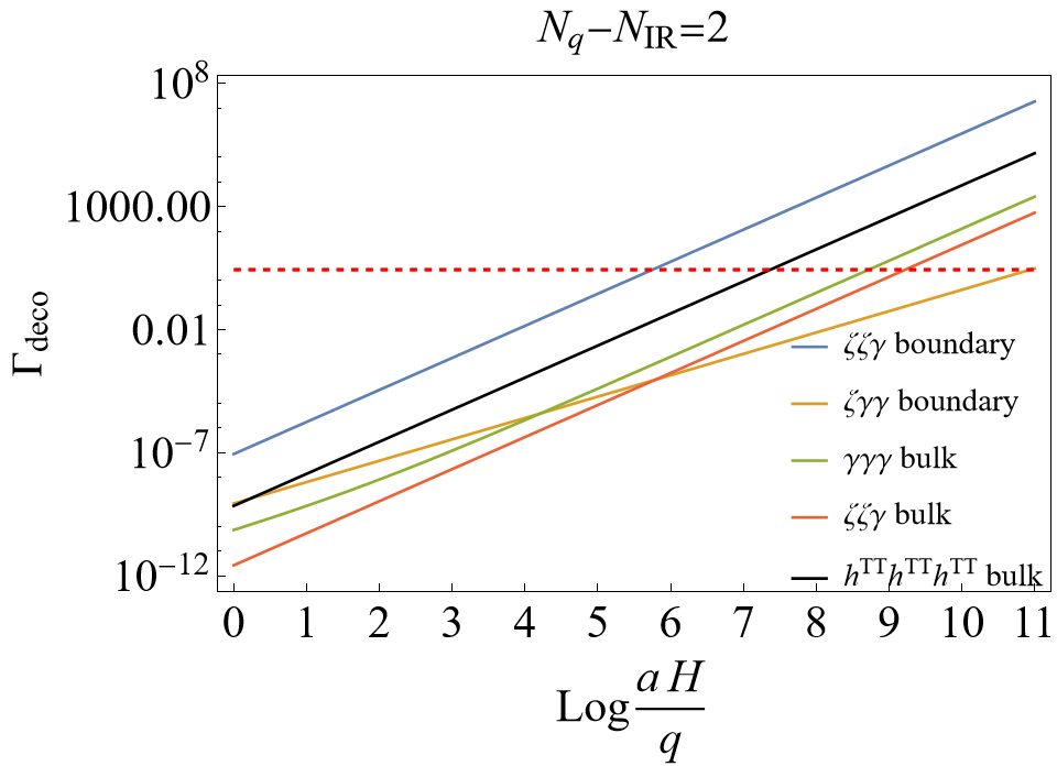
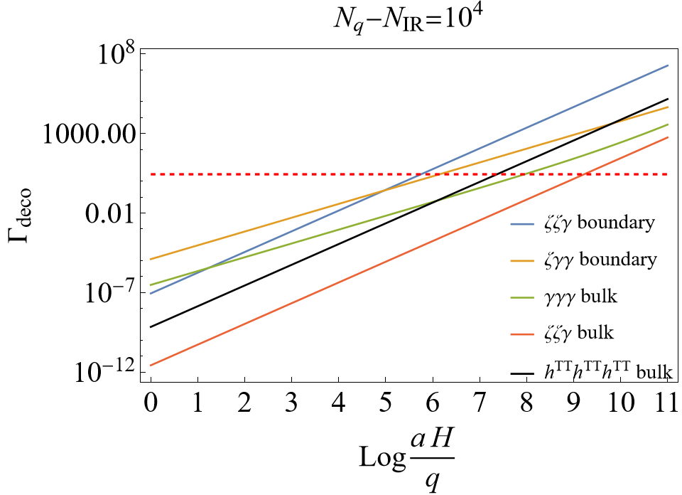
Figure 2: The comparison of $\Gamma(q,\tau)$ from different interactions (78), (87), (93), (98) and (100). The red-dashed line indicates $\Gamma(q,\tau)=1$, and the observed values $\Delta_{\zeta}^{2}\approx 2.5\times 10^{-9}$ and $\epsilon<0.006$ are used [83]. Two values of the IR cutoff are chosen: $\Delta N=2$ for the minimal inclusion of the IR environment, and $\Delta N=10^{4}$ as the value used in [36].

V Comments on the one-loop quantum correction

Previously, our treatment is limited to the tree-level analysis, and it remains to be seen how quantum fluctuation will influence the result. Since gravity can be viewed as a non-abelian gauge theory with diffeomorphism invariance, we need to also include ghost fields. In this section, we give an argument that the effect of one-loop correction is neglectable compared to the leading order contribution.

To begin with, following (7), the corresponding Euclidean action reads

$$I[g,\phi]=\int d^{4}x\ \mathcal{L}$$

$$=\int_{\mathcal{M}}d^{4}x\sqrt{g}\left[-\frac{M_{p}^{2}}{2}R-\frac{1}{2}g^{\mu\nu}\partial_{\mu}\phi\partial_{\nu}\phi+V(\phi)\right]-\int_{\partial\mathcal{M}}d^{3}xM_{p}^{2}\sqrt{h}K\ ,\quad\mu,\nu=1,2,3,4$$ (101)

and the wave functional can be expressed with the path integral

$$\Psi(h,\phi_{0})=\int_{g|_{\partial\mathcal{M}}=h,\ \phi|_{\partial\mathcal{M}}=\phi_{0}}\mathcal{D}g\mathcal{D}\phi\ e^{-I[g,\phi]}\ ,$$ (102)

where $h$ and $\phi_{0}$ simply denote the boundary values of the metric and inflation field. The metric and inflation field can be expanded as

$$g=g_{c}+\tilde{h}\ ,\quad\phi=\phi_{c}+\varphi\ ,$$ (103)

where $g_{c}$ and $\phi_{c}$ are the solutions to the classical equations of motion

$$\frac{\delta I[g,\phi]}{\delta g}=0\ ,\quad\frac{\delta I[g,\phi]}{\delta\phi}=0\ ,$$ (104)

and under the diffeomorphism $x_{\mu}\rightarrow x_{\mu}+\xi_{\mu}$ the perturbations transform as

$$\tilde{h}_{\mu\nu}\rightarrow\tilde{h}_{\mu\nu}+\nabla_{\mu}\xi_{\nu}+\nabla_{\nu}\xi_{\mu}\ ,\quad\varphi\rightarrow\varphi-\xi^{\mu}\nabla_{\mu}\varphi\ .$$ (105)

Following [85, 53], the boundary condition here is subtle. Here we mainly focus on metric field because it is the quantum gravity that cause the subtleties instead of scalar field. Usually there are two boundary conditions for metric field, one is the Dirichlet boundary condition, which fixes the metric at the boundary and requires $\tilde{h}|_{\partial\mathcal{M}}=0$, $\xi|_{\partial\mathcal{M}}=0$, so the transverse component of metric is unrestricted and needs gauge fixing. The other is called conformal boundary condition which admits the boundary metric up to a Weyl rescaling. In [85], the author points out that mathematically, the Dirichlet boundary condition will be problematic because this boundary condition breaks the elliptic properties of propagator, and therefore, may not lead to a well-defined perturbation theory of quantum gravity. The conformal boundary condition will satisfy the elliptic properties. However, the author also said that, a sufficient condition for the Dirichlet boundary continues to work is that the extrinsic curvature $K_{ij}$ is either positive or negative definite. For de Sitter it is not hard to prove that the metric satisfies this condition, and therefore both the Dirichlet and conformal boundary condition will work for the analysis.

Without loss of generality, we take the Dirichlet boundary condition, and we need to fix the transverse component of the metric. Following [84], the gauge condition reads:

$$C_{\alpha}={g_{c}}^{\frac{1}{4}}\left(\nabla_{\nu}\tilde{h}^{\nu}_{\mu}-\frac{1}{2}\nabla_{\mu}\tilde{h}-\varphi\nabla_{\mu}\phi_{c}\right)t^{\mu}_{\alpha}=0,\quad\alpha=1,2,3,4$$ (106)

where $t^{\mu}_{\alpha}t^{\alpha\nu}=g_{c}^{\mu\nu}$. It is worthy to note that some references [86, 87] also take the Landau gauge. For the on-shell effective action, different choices of $C_{\alpha}$ are equivalent, whereas for the off-shell effective action, the one-loop correction depends on the choice of gauge. However, we will show that in our case, higher loop corrections can be neglected, and therefore it is reasonable to only consider the on-shell effective action, in which the choice of gauge will not influence our conclusion.

By expanding (106) around an infinitesimal gauge transformation, following [84], the ghost Lagrangian density for one loop is given as:

$$\mathcal{L}_{\rm ghost}=\sqrt{g_{c}}\bar{c}^{\mu}\left(\nabla_{a}\nabla^{a}\delta_{\mu}^{\nu}-R_{\mu}^{\nu}-\nabla^{\nu}\phi_{c}\nabla_{\mu}\phi_{c}\right)c_{v}=\sqrt{g_{c}}\bar{c}^{\mu}J_{\mu}^{\nu}c_{\nu}\ ,$$ (107)

where $c$ and $\bar{c}$ are ghost and anti-ghost fields respectively, which obey the Dirichlet boundary condition and (106). Then we expand (101) to the second order of the metric and inflation field and adding the gauge-fixing term, following [84]

$$\mathcal{L}_{\rm gf}=\mathcal{L}-\frac{1}{2}C_{\mu}C^{\mu} =\sqrt{g_{c}}\Bigg{(}-\frac{1}{4}\tilde{h}^{\beta}_{\alpha,\nu}\tilde{h}^{\alpha,\nu}_{\beta}+\frac{1}{8}\tilde{h}^{\alpha}_{\alpha,\nu}\tilde{h}^{\beta,\nu}_{\beta}-\frac{1}{2}\nabla_{\mu}\varphi\nabla^{\mu}\varphi$$ (108)

$$+\frac{1}{2}\tilde{h}_{\beta}^{\alpha}X_{\alpha\nu}^{\beta\mu}\tilde{h}_{\mu}^{\nu}+\varphi Y_{\beta}^{\alpha}\tilde{h}_{\alpha}^{\beta}+\frac{1}{2}\varphi Z\varphi\Bigg{)}\ ,$$

where the definitions of $X,Y,Z$ are given in [84]:

$$X_{\alpha\nu}^{\beta\mu} =2\Bigg{\{}-\frac{1}{2}\delta_{\nu}^{\beta}\nabla^{\mu}\phi_{c}\nabla_{\alpha}\phi_{c}+\frac{1}{4}\delta_{\alpha}^{\beta}\nabla^{\mu}\phi_{c}\nabla_{\nu}\phi_{c}-\frac{1}{16}\delta_{\alpha}^{\beta}\delta_{\nu}^{\mu}\left[\nabla_{\gamma}\phi_{c}\nabla^{\gamma}\phi_{c}+2V(\phi_{c})\right]$$ (109)

$$+\frac{1}{8}\delta_{\nu}^{\beta}\delta_{\alpha}^{\mu}\left[\nabla_{\gamma}\phi_{c}\nabla^{\gamma}\phi_{c}+2V(\phi_{c})\right]-\frac{1}{8}\delta_{\alpha}^{\beta}\delta_{\nu}^{\mu}R+\frac{1}{4}\delta^{\beta}_{\nu}\delta_{\alpha}^{\mu}R$$

$$-\frac{1}{2}\delta_{\nu}^{\beta}R_{\alpha}^{\mu}+\frac{1}{2}\delta_{\alpha}^{\beta}R_{\nu}^{\mu}+\frac{1}{2}R^{\beta\mu}_{\quad\alpha\nu}\Bigg{\}},$$

$$Y_{\beta}^{\alpha} =\frac{1}{2}\delta_{\beta}^{\alpha}\nabla_{\nu}\nabla^{\nu}\phi_{c}-\nabla_{\beta}\nabla^{\alpha}\phi_{c}+\frac{1}{2}\frac{\delta V}{\delta\phi}\Big{|}_{\phi=\phi_{c}}\delta^{\alpha}_{\beta},$$

$$Z =-\nabla_{\mu}\phi_{c}\nabla^{\mu}\phi_{c}+\frac{1}{2}\frac{\partial^{2}V}{\partial\phi^{2}}\Big{|}_{\phi=\phi_{c}}\ ,$$

and we used the facts that:

$$\delta\sqrt{g}=\frac{1}{2}\sqrt{g_{c}}\tilde{h}_{\alpha}^{\alpha}+\frac{1}{4}\sqrt{g_{c}}\left[-\tilde{h}^{\alpha}_{\beta}\tilde{h}^{\beta}_{\alpha}+\frac{1}{2}(\tilde{h}^{\alpha}_{\alpha})^{2}\right]\ ,$$ (110)

and

$$\delta V(\phi)=\frac{\partial V}{\partial\phi}\Big{|}_{\phi=\phi_{c}}\varphi+\frac{1}{2}\frac{\partial^{2}V}{\partial\phi^{2}}\Big{|}_{\phi=\phi_{c}}\varphi^{2}\ .$$ (111)

Following [88, 65], the one-loop wave functional is then formally written as:

$$\Psi_{{\rm 1-loop}}=\frac{\text{det}{\bf J}}{(\text{det}{\bf G})^{\frac{1}{2}}}e^{-I[\phi_{c},g_{c}]}=e^{-I_{\rm eff}[\phi_{c},g_{c}]}\ ,$$ (112)

where ${\bf J}$ is defined in (107), and ${\bf G}$ is defined as:

$${\bf G}=\begin{pmatrix}\frac{\delta^{2}\mathcal{L}_{\rm gf}}{\delta^{2}\tilde{h}_{\alpha\beta}\tilde{h}_{\mu\nu}}&&\frac{\delta^{2}\mathcal{L}_{\rm gf}}{\delta\tilde{h}_{\mu\nu}\delta\varphi}\\ \frac{\delta^{2}\mathcal{L}_{\rm gf}}{\delta\tilde{h}_{\alpha\beta}\delta\varphi}&&\frac{\delta^{2}\mathcal{L}_{\rm gf}}{\delta\varphi^{2}}\end{pmatrix}\ ,$$ (113)

and the effective action is written as:

$$I_{\rm eff}[\phi_{c},g_{c}]=I[\phi_{c},g_{c}]-\text{Tr}\log{\bf J}[\phi_{c},g_{c}]+\frac{1}{2}\text{Tr}\log{\bf G}[\phi_{c},g_{c}]\ .$$ (114)

The explicit calculation of the determinants needs to use the zeta function regulator and is model dependent, because here we need to know the explicit form of inflaton potential $V(\phi)$. The results have been shown in various literature, for reference, see [69, 89, 90, 86, 87]. Here we take the example in [86]: the effective action for a pure gravity with de Sitter background has the form

$$I_{\rm eff}\sim\int d^{4}x\sqrt{g}\left[-\frac{M_{p}^{2}}{2}(R-2\Lambda)+R^{2}\log\left(\frac{R}{\mu^{2}}\right)\right]\ ,$$ (115)

where the first term is tree-level, and the second term is the one-loop correction with a energy scale $\mu$. For the de Sitter space with $R=4\Lambda=12H^{2}$, the ratio of the one-loop to tree-level contributions is:

$$\frac{I_{\rm 1-loop}}{I_{\rm tree}} \sim\frac{H^{2}}{M_{p}^{2}}\log\frac{R}{\mu^{2}}\sim\Delta^{2}_{\gamma}\lesssim\mathcal{O}\left(10^{-10}\right)\ ,$$ (116)

where the energy scale is chosen as $\mu\sim H$, and the Planck data [83] is used for the estimation. Similar form of the one-loop correction (115) is also derived in explicit inflation models such as [87], so the order estimation (116) should be generic. Such a small ratio implies that the one-loop and higher-order corrections to the phase of wave functional and the corresponding decoherence effect are neglectable.

Following [91, 92, 93, 94], it is worthy to mention that the symmetry also allows some other one-loop corrections, take the two-point function of scalar curvature perturbation as an example, there are two possible terms that allowed by symmetry. One is:

$$\langle\zeta_{p}^{2}\rangle_{\rm 1-loop}\sim p^{3}\langle\zeta_{p}^{2}\rangle_{\rm tree}^{2}\log(pL)\ ,$$ (117)

where $L$ being the comoving size, and the other is:

$$\langle\zeta_{p}^{2}\rangle_{\rm 1-loop}\sim p^{3}\langle\zeta_{p}^{2}\rangle_{\rm tree}^{2}\log(a(t))\ .$$ (118)

The first term might contribute large in the IR limit, however, [94] shows that this will not affect the observable quantities and is purely a projection effect. The second term is only logarithmic type with the suppression of $\Delta^{2}_{\zeta}$ that it will not influence the result significantly as well. Similarly, the one-loop correction of gravitons’ two-point function also includes a logarithmic term like [95]

$$\left\langle\left(h^{\rm TT}_{p}\right)^{2}\right\rangle_{\rm 1-loop}\sim p^{3}\left\langle\left(h^{\rm TT}_{p}\right)^{2}\right\rangle_{\rm tree}^{2}\log(a(t))\ ,$$ (119)

which also does not correct significantly to the result, following the reason of the scalar case.

VI Conclusion

Studying the decoherence of primordial gravitons is not only for explaining the quantum-to-classical transition of the primordial gravitational wave, but it is also useful to set constraints and identify potential obstacles for probing the non-classicality of squeezed gravitons. In this paper, we proceeded the discussion of the slow-roll unsuppressed boundary-term decoherence in [41] and calculated the case with primordial gravitons.

Starting from the standard procedure of splitting the bulk and boundary interaction terms with integration by parts, we confirmed that there exists unsuppressed scalar-tensor coupling boundary terms of $\zeta$ and $\gamma_{ij}$. Such boundary terms were shown to contribute a non-Gaussian phase to the wave functional of cosmological perturbations with either the interaction and Schrödinger picture approaches. As the phase grows with the scale factor $a(t)$, the corresponding quantum state is close to the WKB type, as expected in [34], but now we have showed that it is slow-roll unsuppressed.

To gain insight into the unsuppressed phase of the wave functional, we studied the Wheeler-DeWitt formalism of quantum gravity with the WKB approximation valid in the large $a(t)$ limit. The WKB phase evaluated on the hypersurface with the given $(h_{ij},\phi)$ was shown to include unsuppressed cubic terms, agreeing with those obtained from the boundary terms. This result suggests that the leading phase of the inflationary wave functional is independent to the bulk-boundary splitting of the action, but such a splitting is certainly helpful to identify the unsuppressed terms. The agreement of these approaches also suggests that full considerations of either the boundary terms of cosmological perturbations or the WKB limit of the WDW wave functional are needed to discuss the classicalization of the perturbations.

We thus calculated the environment-induced decoherence of primordial gravitons with the wave functional method presented in [34], addressing the influence by the unsuppressed non-Gaussian phase. The gravitons were shown to decohere around 5-6 e-folds after crossing the horizon, faster than the process by the bulk interactions which takes 7-9 e-folds. We have also estimated the size of the one-loop quantum correction to the wave functional including the Faddeev-Popov ghost determinant, showing that it is suppressed by a factor of graviton’s power spectrum $\frac{H^{2}}{M_{p}^{2}}$ compared to the three-level part, so the correction to our results should be negligible. During inflation, the squeezing of primordial gravitons happens after the horizon crossing with the parameter grows as $R_{q}\sim\log\left(\frac{aH}{q}\right)$ [3], so their purity should also be considered in the proposals testing their non-classicality. How exactly the cosmological decoherence affects the proposals deserves further studies.

Finally, we comment on the relationship between the physical hypersurface $\Sigma$ and decoherence. As demonstrated in [41] with the well-defined variational principle, the boundary terms on the two hypersurfaces naturally defined in the $\zeta$-gauge and $\delta\phi$-gauge respectively are different, whereas they become equal when the same $\Sigma$ is chosen even if the calculation is done with the fields defined in different gauges. It is noteworthy that similar results have been reported in [50] by constructing gauge-invariant quantities for all the scalar and tensor interactions, and boundary terms on different hypersurfaces do not match even the non-linear field redefinition is considered. Here we make another point of view by studying the phase of the WDW wave functional, and the leading WKB phase $W(h_{ij},\phi)$ is evaluated by choosing $\Sigma$. By the relationship between the phase of wave functional and boundary terms, it is easy to verify the facts in [50, 41]. This also implies the same conclusion in [41] that the quantities naturally defined on various $\Sigma$ have different decoherence rates, such as $\zeta$ and $\gamma_{ij}$ which conserve on super-horizon scales decohere faster. Better understanding the physical meanings of these conclusions is also worthy for further studies. Following [67, 96], it will also be interesting to understand the decoherence effect in this paper from the perspective of dS/CFT and AdS/CFT, and in the context of string cosmology [97]. We leave this for future work.

Appendix A The analytical expressions of $J_{\zeta\zeta\gamma}(Q)$ and $J_{\zeta\gamma\gamma}(Q)$

The expression of $J_{\zeta\zeta\gamma}$ in (78) is

$$J_{\zeta\zeta\gamma}(Q)=-\frac{1}{3840\pi^{2}Q^{5}}\Bigg{\{}8\left(15Q^{6}+90Q^{4}+80Q^{2}+48\right)\log\left(Q^{2}+1\right)$$

$$-8Q^{2}\left[15\pi Q^{5}-30Q^{4}-28\pi Q^{3}+56Q^{2}+\left(56Q^{3}-30Q^{5}\right)\tan^{-1}(Q)+48\right]$$

$$+15Q^{4}\left(Q^{2}+4\right)^{2}\Bigg{[}\text{Li}_{2}\left(\frac{Q(Q-i)}{Q^{2}-iQ+2}\right)+\text{Li}_{2}\left(\frac{Q(Q+i)}{Q^{2}+iQ+2}\right)-\text{Li}_{2}\left(\frac{Q^{2}+iQ+2}{Q^{2}+iQ}\right)$$

$$+2\text{Li}_{2}\left(\frac{2i}{Q}-1\right)-\text{Li}_{2}\left(\frac{Q}{Q-2i}\right)-\text{Li}_{2}\left(\frac{Q-2i}{Q}\right)-\text{Li}_{2}\left(\frac{(Q+i)(Q-2i)}{Q(Q-i)}\right)$$

$$-2\text{Li}_{2}\left(-\frac{Q}{Q+2i}\right)+\text{Li}_{2}\left(\frac{Q}{Q+2i}\right)+\text{Li}_{2}\left(\frac{Q+2i}{Q}\right)+2i\log\left(\frac{2}{Q^{2}-iQ+2}\right)\tan^{-1}(Q)$$

$$-2i\log\left(-\frac{2}{Q^{2}+iQ}\right)\tan^{-1}(Q)-2i\log\left(\frac{2}{Q^{2}+iQ+2}\right)\tan^{-1}(Q)+i\pi\log\left(-\frac{2i}{Q}\right)$$

$$-i\pi\log\left(\frac{2i}{Q}\right)-i\pi\log\left(-\frac{2i}{Q-2i}\right)+i\pi\log\left(\frac{2i}{Q+2i}\right)+2i\log\left(-\frac{2}{Q(Q-i)}\right)\tan^{-1}(Q)$$

$$+\mathcal{T}_{\zeta\zeta\gamma}^{+}(Q)\tanh^{-1}(1+iQ)+\mathcal{T}_{\zeta\zeta\gamma}^{-}(Q)\tanh^{-1}(1-iQ)\Bigg{]}\Bigg{\}}\ ,$$ (120)

where

$$\mathcal{T}_{\zeta\zeta\gamma}^{+}(Q) =-\log\left(4Q(Q-2i)\left(Q^{2}+1\right)\right)+2\log\left(-\frac{i}{\sqrt{Q(Q-2i)\left(Q^{2}+1\right)}}\right)+2\log(-1+iQ)$$

$$+2\log(2+iQ)+4\log(2+2iQ)+2\log(Q-i)+2\log\left(\frac{i}{2(Q-2i)}\right)$$

$$-4\log\left(\frac{Q-i}{\sqrt{Q(Q-2i)}}\right)-4i\pi\ ,$$

$$\mathcal{T}_{\zeta\zeta\gamma}^{-}(Q) =4\log(1-iQ)+2\log(Q+i)-2\log\left(\frac{2i}{Q+2i}\right)-4\log\left(\frac{Q+i}{\sqrt{Q+2i}}\right)$$

$$+2\log\left(\frac{i}{2\sqrt{Q+i}\sqrt{2+Q(Q+i)}}\right)+2\log\left(-\frac{4i}{\sqrt{Q+i}\sqrt{2+Q(Q+i)}}\right)$$

$$-4\tanh^{-1}\left(\frac{1}{3}-\frac{2iQ}{3}\right)-3i\pi\ .$$ (121)

On the other hand, $J_{\zeta\gamma\gamma}(Q)$ defined in (87) is

$$J_{\zeta\gamma\gamma}(Q)=-\frac{1}{1935360\pi^{2}Q^{6}\left(Q^{2}+1\right)}\Bigg{\{}$$

$$24\left(315Q^{12}-7875Q^{10}+13650Q^{8}-23835Q^{6}+82296Q^{4}-32491Q^{2}+818\right)\log\left(Q^{2}+1\right)$$

$$-16\Bigg{[}9984+43008Q^{2}+\Bigg{(}3\pi Q\left(315Q^{6}-10225Q^{4}+44756Q^{2}-25344\right)$$

$$-2\left(945Q^{6}-30675Q^{4}+135988Q^{2}+151096\right)\Bigg{)}Q^{4}\Bigg{]}Q^{2}$$

$$+\mathcal{T}_{\zeta\gamma\gamma}(Q)\log(1+iQ)+\mathcal{T}^{*}_{\zeta\gamma\gamma}(Q)\log(1-iQ)+945Q^{8}\left(Q^{6}-23Q^{4}-8Q^{2}+16\right)\Bigg{[}4\text{Li}_{2}\left(-\frac{i}{Q}\right)$$

$$+4\text{Li}_{2}\left(\frac{i}{Q}\right)-4\text{Li}_{2}\left(\frac{Q-i}{Q}\right)-4\text{Li}_{2}\left(\frac{Q+i}{Q}\right)-4\text{Li}_{2}\left(-\frac{i}{Q-2i}\right)+4\text{Li}_{2}\left(\frac{Q-i}{Q-2i}\right)$$

$$-4\text{Li}_{2}\left(\frac{i}{Q+2i}\right)+4\text{Li}_{2}\left(\frac{Q+i}{Q+2i}\right)+\log^{2}(-Q-2i)+\log^{2}(-Q+2i)-\log^{2}(Q-2i)$$

$$-\log^{2}(Q+2i)-i\pi\log(-Q-2i)+i\pi\log(-Q+2i)+i\pi\log(Q-2i)-i\pi\log(Q+2i)\Bigg{]}\Bigg{\}}\ ,$$ (122)

where

$$\mathcal{T}_{\zeta\gamma\gamma}(Q) =6\Bigg{[}-315i\pi Q^{14}-2520iQ^{13}+(1260+7245i\pi)Q^{12}+81800iQ^{11}$$

$$+(-31500+2520i\pi)Q^{10}-358048iQ^{9}+(54600-5040i\pi)Q^{8}+202752iQ^{7}$$

$$+471660Q^{6}+618912Q^{4}+257964Q^{2}+23352$$

$$+630\left(Q^{6}-23Q^{4}-8Q^{2}+16\right)Q^{8}\log(Q)$$

$$+630\left(Q^{6}-23Q^{4}-8Q^{2}+16\right)Q^{8}\log\left(-\frac{i}{Q-2i}\right)\Bigg{]}\ .$$ (123)

The two functions have real values on $0<Q=\frac{q}{aH}<1$, shown in Fig 3.

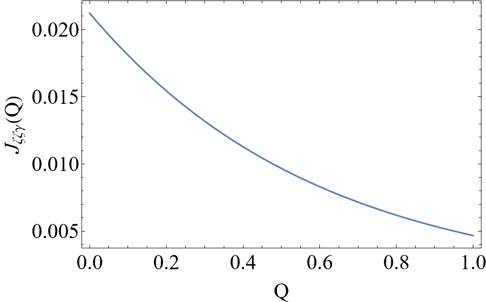
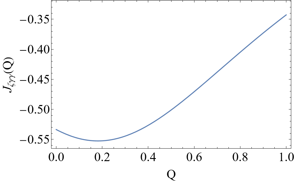
Figure 3: $J_{\zeta\zeta\gamma}\left(Q\right)$ and $J_{\zeta\gamma\gamma}\left(Q\right)$ defined in (78) and (87) respectively.

References

- [1] L. P. Grishchuk and Y. V. Sidorov, “On the Quantum State of Relic Gravitons,” Class. Quant. Grav. 6 (1989) L161–L165.
- [2] L. P. Grishchuk and Y. V. Sidorov, “Squeezed quantum states of relic gravitons and primordial density fluctuations,” Phys. Rev. D 42 (1990) 3413–3421.
- [3] A. Albrecht, P. Ferreira, M. Joyce, and T. Prokopec, “Inflation and squeezed quantum states,” Phys. Rev. D 50 (1994) 4807–4820, arXiv:astro-ph/9303001.
- [4] D. Polarski and A. A. Starobinsky, “Semiclassicality and decoherence of cosmological perturbations,” Class. Quant. Grav. 13 (1996) 377–392, arXiv:gr-qc/9504030.
- [5] M. Parikh, F. Wilczek, and G. Zahariade, “The Noise of Gravitons,” Int. J. Mod. Phys. D 29 no. 14, (2020) 2042001, arXiv:2005.07211 [hep-th].
- [6] M. Parikh, F. Wilczek, and G. Zahariade, “Signatures of the quantization of gravity at gravitational wave detectors,” Phys. Rev. D 104 no. 4, (2021) 046021, arXiv:2010.08208 [hep-th].
- [7] M. Parikh, F. Wilczek, and G. Zahariade, “Quantum Mechanics of Gravitational Waves,” Phys. Rev. Lett. 127 no. 8, (2021) 081602, arXiv:2010.08205 [hep-th].
- [8] S. Kanno, J. Soda, and J. Tokuda, “Noise and decoherence induced by gravitons,” Phys. Rev. D 103 no. 4, (2021) 044017, arXiv:2007.09838 [hep-th].
- [9] Z. Haba, “State-dependent graviton noise in the equation of geodesic deviation,” Eur. Phys. J. C 81 no. 1, (2021) 40, arXiv:2009.12306 [gr-qc].
- [10] H.-T. Cho and B.-L. Hu, “Quantum noise of gravitons and stochastic force on geodesic separation,” Phys. Rev. D 105 no. 8, (2022) 086004, arXiv:2112.08174 [gr-qc].
- [11] S.-E. Bak, M. Parikh, S. Sarkar, and F. Setti, “Quantum Gravity Fluctuations in the Timelike Raychaudhuri Equation,” arXiv:2212.14010 [gr-qc].
- [12] H.-T. Cho and B.-L. Hu, “Graviton noise on tidal forces and geodesic congruences,” Phys. Rev. D 107 no. 8, (2023) 084005, arXiv:2301.06325 [gr-qc].
- [13] E. Calzetta and B. L. Hu, “Noise and fluctuations in semiclassical gravity,” Phys. Rev. D 49 (1994) 6636–6655, arXiv:gr-qc/9312036.
- [14] B. L. Hu, “Stochastic gravity,” Int. J. Theor. Phys. 38 (1999) 2987–3037, arXiv:gr-qc/9902064.
- [15] B. L. Hu and E. Verdaguer, “Stochastic Gravity: Theory and Applications,” Living Rev. Rel. 11 (2008) 3, arXiv:0802.0658 [gr-qc].
- [16] M. P. Hertzberg and J. A. Litterer, “Bound on quantum fluctuations in gravitational waves from LIGO-Virgo,” JCAP 03 (2023) 009, arXiv:2112.12159 [gr-qc].
- [17] S. Kanno, J. Soda, and J. Tokuda, “Indirect detection of gravitons through quantum entanglement,” Phys. Rev. D 104 no. 8, (2021) 083516, arXiv:2103.17053 [gr-qc].
- [18] F. S. Arani, M. B. Harouni, B. Lamine, and A. Blanchard, “Sensing quantum nature of primordial gravitational waves using electromagnetic probes,” Phys. Scripta 98 no. 5, (2023) 055004, arXiv:2110.10962 [gr-qc].
- [19] M. Giovannini, “Hanbury Brown-Twiss interferometry and second-order correlations of inflaton quanta,” Phys. Rev. D 83 (2011) 023515, arXiv:1011.1673 [astro-ph.CO].
- [20] S. Kanno and J. Soda, “Detecting nonclassical primordial gravitational waves with Hanbury-Brown–Twiss interferometry,” Phys. Rev. D 99 no. 8, (2019) 084010, arXiv:1810.07604 [hep-th].
- [21] S. Kanno, “Nonclassical primordial gravitational waves from the initial entangled state,” Phys. Rev. D 100 no. 12, (2019) 123536, arXiv:1905.06800 [hep-th].
- [22] T. Guerreiro, “Quantum Effects in Gravity Waves,” Class. Quant. Grav. 37 no. 15, (2020) 155001, arXiv:1911.11593 [quant-ph].
- [23] T. Guerreiro, F. Coradeschi, A. M. Frassino, J. R. West, and E. Schioppa, Junior., “Quantum signatures in nonlinear gravitational waves,” Quantum 6 (2022) 879, arXiv:2111.01779 [gr-qc].
- [24] B. L. Hu, J. P. Paz, and Y. Zhang, “Quantum origin of noise and fluctuations in cosmology,” in The Origin of Structure in the Universe. 1992. arXiv:gr-qc/9512049.
- [25] E. Calzetta and B. L. Hu, “Quantum fluctuations, decoherence of the mean field, and structure formation in the early universe,” Phys. Rev. D 52 (1995) 6770–6788, arXiv:gr-qc/9505046.
- [26] F. C. Lombardo and D. Lopez Nacir, “Decoherence during inflation: The Generation of classical inhomogeneities,” Phys. Rev. D 72 (2005) 063506, arXiv:gr-qc/0506051.
- [27] C. Kiefer, I. Lohmar, D. Polarski, and A. A. Starobinsky, “Pointer states for primordial fluctuations in inflationary cosmology,” Class. Quant. Grav. 24 (2007) 1699–1718, arXiv:astro-ph/0610700.
- [28] C. Kiefer and D. Polarski, “Why do cosmological perturbations look classical to us?,” Adv. Sci. Lett. 2 (2009) 164–173, arXiv:0810.0087 [astro-ph].
- [29] C. P. Burgess, R. Holman, and D. Hoover, “Decoherence of inflationary primordial fluctuations,” Phys. Rev. D 77 (2008) 063534, arXiv:astro-ph/0601646.
- [30] P. Martineau, “On the decoherence of primordial fluctuations during inflation,” Class. Quant. Grav. 24 (2007) 5817–5834, arXiv:astro-ph/0601134.
- [31] T. Prokopec and G. I. Rigopoulos, “Decoherence from Isocurvature perturbations in Inflation,” JCAP 11 (2007) 029, arXiv:astro-ph/0612067.
- [32] C. P. Burgess, R. Holman, G. Tasinato, and M. Williams, “EFT Beyond the Horizon: Stochastic Inflation and How Primordial Quantum Fluctuations Go Classical,” JHEP 03 (2015) 090, arXiv:1408.5002 [hep-th].
- [33] D. Boyanovsky, “Effective field theory during inflation: Reduced density matrix and its quantum master equation,” Phys. Rev. D 92 no. 2, (2015) 023527, arXiv:1506.07395 [astro-ph.CO].
- [34] E. Nelson, “Quantum Decoherence During Inflation from Gravitational Nonlinearities,” JCAP 03 (2016) 022, arXiv:1601.03734 [gr-qc].
- [35] S. Shandera, N. Agarwal, and A. Kamal, “Open quantum cosmological system,” Phys. Rev. D 98 no. 8, (2018) 083535, arXiv:1708.00493 [hep-th].
- [36] J. Martin and V. Vennin, “Observational constraints on quantum decoherence during inflation,” JCAP 05 (2018) 063, arXiv:1801.09949 [astro-ph.CO].
- [37] J. Martin and V. Vennin, “Non Gaussianities from Quantum Decoherence during Inflation,” JCAP 06 (2018) 037, arXiv:1805.05609 [astro-ph.CO].
- [38] A. Daddi Hammou and N. Bartolo, “Cosmic decoherence: primordial power spectra and non-Gaussianities,” arXiv:2211.07598 [astro-ph.CO].
- [39] T. Colas, J. Grain, and V. Vennin, “Benchmarking the cosmological master equations,” Eur. Phys. J. C 82 no. 12, (2022) 1085, arXiv:2209.01929 [hep-th].
- [40] G. Ye and Y.-S. Piao, “Quantum decoherence of primordial perturbations through nonlinear scaler-tensor interaction,” arXiv:1806.07672 [gr-qc].
- [41] C. M. Sou, D. H. Tran, and Y. Wang, “Decoherence of cosmological perturbations from boundary terms and the non-classicality of gravity,” JHEP 04 (2023) 092, arXiv:2207.04435 [hep-th].
- [42] P. Friedrich and T. Prokopec, “Entropy production in inflation from spectator loops,” Phys. Rev. D 100 no. 8, (2019) 083505, arXiv:1907.13564 [astro-ph.CO].
- [43] S. Brahma, O. Alaryani, and R. Brandenberger, “Entanglement entropy of cosmological perturbations,” Phys. Rev. D 102 no. 4, (2020) 043529, arXiv:2005.09688 [hep-th].
- [44] J.-O. Gong and M.-S. Seo, “Quantum non-linear evolution of inflationary tensor perturbations,” JHEP 05 (2019) 021, arXiv:1903.12295 [hep-th].
- [45] C. P. Burgess, R. Holman, G. Kaplanek, J. Martin, and V. Vennin, “Minimal decoherence from inflation,” arXiv:2211.11046 [hep-th].
- [46] S. Kanno, J. Soda, and K. Ueda, “Conversion of squeezed gravitons into photons during inflation,” Phys. Rev. D 106 no. 8, (2022) 083508, arXiv:2207.05734 [hep-th].
- [47] S. Kanno, J. Soda, and K. Ueda, “Impact of quantum entanglement induced by magnetic fields on primordial gravitational waves,” arXiv:2211.05576 [hep-th].
- [48] F. Arroja and T. Tanaka, “A note on the role of the boundary terms for the non-Gaussianity in general k-inflation,” JCAP 05 (2011) 005, arXiv:1103.1102 [astro-ph.CO].
- [49] C. Burrage, R. H. Ribeiro, and D. Seery, “Large slow-roll corrections to the bispectrum of noncanonical inflation,” JCAP 07 (2011) 032, arXiv:1103.4126 [astro-ph.CO].
- [50] T. Prokopec and J. Weenink, “Frame independent cosmological perturbations,” JCAP 09 (2013) 027, arXiv:1304.6737 [gr-qc].
- [51] B. S. DeWitt, “Quantum Theory of Gravity. 1. The Canonical Theory,” Phys. Rev. 160 (1967) 1113–1148.
- [52] J. A. Wheeler, “SUPERSPACE AND THE NATURE OF QUANTUM GEOMETRODYNAMICS,” Adv. Ser. Astrophys. Cosmol. 3 (1987) 27–92.
- [53] E. Witten, “A Note On The Canonical Formalism for Gravity,” arXiv:2212.08270 [hep-th].
- [54] G. Araujo-Regado, R. Khan, and A. C. Wall, “Cauchy slice holography: a new AdS/CFT dictionary,” JHEP 03 (2023) 026, arXiv:2204.00591 [hep-th].
- [55] L. McGough, M. Mezei, and H. Verlinde, “Moving the CFT into the bulk with ,” JHEP 04 (2018) 010, arXiv:1611.03470 [hep-th].
- [56] T. Hartman, J. Kruthoff, E. Shaghoulian, and A. Tajdini, “Holography at finite cutoff with a deformation,” JHEP 03 (2019) 004, arXiv:1807.11401 [hep-th].
- [57] G. Araujo-Regado, “Holographic Cosmology on Closed Slices in 2+1 Dimensions,” arXiv:2212.03219 [hep-th].
- [58] F. Larsen and R. McNees, “Holography, diffeomorphisms, and scaling violations in the CMB,” JHEP 07 (2004) 062, arXiv:hep-th/0402050.
- [59] G. L. Pimentel, “Inflationary Consistency Conditions from a Wavefunctional Perspective,” JHEP 02 (2014) 124, arXiv:1309.1793 [hep-th].
- [60] E. Pajer, G. L. Pimentel, and J. V. S. Van Wijck, “The Conformal Limit of Inflation in the Era of CMB Polarimetry,” JCAP 06 (2017) 009, arXiv:1609.06993 [hep-th].
- [61] F. Larsen and R. McNees, “Inflation and de Sitter holography,” JHEP 07 (2003) 051, arXiv:hep-th/0307026.
- [62] J. Maldacena, G. J. Turiaci, and Z. Yang, “Two dimensional Nearly de Sitter gravity,” JHEP 01 (2021) 139, arXiv:1904.01911 [hep-th].
- [63] T. Chakraborty, J. Chakravarty, V. Godet, P. Paul, and S. Raju, “The Hilbert space of de Sitter quantum gravity,” arXiv:2303.16315 [hep-th].
- [64] T. Chakraborty, J. Chakravarty, V. Godet, P. Paul, and S. Raju, “Holography of information in de Sitter space,” arXiv:2303.16316 [hep-th].
- [65] L. Freidel, “Reconstructing AdS/CFT,” arXiv:0804.0632 [hep-th].
- [66] I. Papadimitriou, “Holographic renormalization as a canonical transformation,” JHEP 11 (2010) 014, arXiv:1007.4592 [hep-th].
- [67] J. M. Maldacena, “Non-Gaussian features of primordial fluctuations in single field inflationary models,” JHEP 05 (2003) 013, arXiv:astro-ph/0210603.
- [68] J. W. York, Jr., “Role of conformal three geometry in the dynamics of gravitation,” Phys. Rev. Lett. 28 (1972) 1082–1085.
- [69] G. W. Gibbons and S. W. Hawking, “Action Integrals and Partition Functions in Quantum Gravity,” Phys. Rev. D 15 (1977) 2752–2756.
- [70] J. York, “Boundary terms in the action principles of general relativity,” Found. Phys. 16 (1986) 249–257.
- [71] T. Prokopec and G. Rigopoulos, “Path Integral for Inflationary Perturbations,” Phys. Rev. D 82 (2010) 023529, arXiv:1004.0882 [gr-qc].
- [72] A. Ota, M. Sasaki, and Y. Wang, “One-loop tensor power spectrum from an excited scalar field during inflation,” arXiv:2211.12766 [astro-ph.CO].
- [73] J. M. Maldacena and G. L. Pimentel, “On graviton non-Gaussianities during inflation,” JHEP 09 (2011) 045, arXiv:1104.2846 [hep-th].
- [74] G. Rigopoulos, “Gauge invariance and non-Gaussianity in Inflation,” Phys. Rev. D 84 (2011) 021301, arXiv:1104.0292 [astro-ph.CO].
- [75] T. Prokopec and J. Weenink, “Uniqueness of the gauge invariant action for cosmological perturbations,” JCAP 12 (2012) 031, arXiv:1209.1701 [gr-qc].
- [76] S. Garcia-Saenz, L. Pinol, and S. Renaux-Petel, “Revisiting non-Gaussianity in multifield inflation with curved field space,” JHEP 01 (2020) 073, arXiv:1907.10403 [hep-th].
- [77] Y. Wang, “MathGR: a tensor and GR computation package to keep it simple,” arXiv:1306.1295 [cs.MS].
- [78] Y. Wang, “Inflation, Cosmic Perturbations and Non-Gaussianities,” Commun. Theor. Phys. 62 (2014) 109–166, arXiv:1303.1523 [hep-th].
- [79] D. S. Salopek and J. M. Stewart, “Hamilton-Jacobi theory for general relativity with matter fields,” Class. Quant. Grav. 9 (1992) 1943–1968.
- [80] J. Parry, D. S. Salopek, and J. M. Stewart, “Solving the Hamilton-Jacobi equation for general relativity,” Phys. Rev. D 49 (1994) 2872–2881, arXiv:gr-qc/9310020.
- [81] J. Liu, C.-M. Sou, and Y. Wang, “Cosmic Decoherence: Massive Fields,” JHEP 10 (2016) 072, arXiv:1608.07909 [hep-th].
- [82] A. O. Barvinsky, A. Y. Kamenshchik, C. Kiefer, and I. V. Mishakov, “Decoherence in quantum cosmology at the onset of inflation,” Nucl. Phys. B 551 (1999) 374–396, arXiv:gr-qc/9812043.
- [83] Planck Collaboration, Y. Akrami et al., “Planck 2018 results. X. Constraints on inflation,” Astron. Astrophys. 641 (2020) A10, arXiv:1807.06211 [astro-ph.CO].
- [84] G. ’t Hooft and M. J. G. Veltman, “One loop divergencies in the theory of gravitation,” Ann. Inst. H. Poincare Phys. Theor. A 20 (1974) 69–94.
- [85] E. Witten, “A note on boundary conditions in Euclidean gravity,” Rev. Math. Phys. 33 no. 10, (2021) 2140004, arXiv:1805.11559 [hep-th].
- [86] E. Fradkin and A. Tseytlin, “One-loop effective potential in gauged o(4) supergravity and the problem of the term,” Nuclear Physics B 234 no. 2, (1984) 472–508.
- [87] K. Bamba, G. Cognola, S. D. Odintsov, and S. Zerbini, “One-loop modified gravity in a de Sitter universe, quantum-corrected inflation, and its confrontation with the Planck result,” Phys. Rev. D 90 no. 2, (2014) 023525, arXiv:1404.4311 [gr-qc].
- [88] A. O. Barvinsky, “Quantum Effective Action in Spacetimes with Branes and Boundaries: Diffeomorphism Invariance,” Phys. Rev. D 74 (2006) 084033, arXiv:hep-th/0608004.
- [89] G. W. Gibbons, S. W. Hawking, and M. J. Perry, “Path Integrals and the Indefiniteness of the Gravitational Action,” Nucl. Phys. B 138 (1978) 141–150.
- [90] S. M. Christensen and M. J. Duff, “Quantizing Gravity with a Cosmological Constant,” Nucl. Phys. B 170 (1980) 480–506.
- [91] S. Weinberg, “Quantum contributions to cosmological correlations,” Phys. Rev. D 72 (2005) 043514, arXiv:hep-th/0506236.
- [92] L. Senatore and M. Zaldarriaga, “On Loops in Inflation,” JHEP 12 (2010) 008, arXiv:0912.2734 [hep-th].
- [93] G. L. Pimentel, L. Senatore, and M. Zaldarriaga, “On Loops in Inflation III: Time Independence of zeta in Single Clock Inflation,” JHEP 07 (2012) 166, arXiv:1203.6651 [hep-th].
- [94] L. Senatore and M. Zaldarriaga, “On Loops in Inflation II: IR Effects in Single Clock Inflation,” JHEP 01 (2013) 109, arXiv:1203.6354 [hep-th].
- [95] S. Brahma, A. Berera, and J. Calderón-Figueroa, “Quantum corrections to the primordial tensor spectrum: open EFTs & Markovian decoupling of UV modes,” JHEP 08 (2022) 225, arXiv:2206.05797 [hep-th].
- [96] A. Del Campo and T. Takayanagi, “Decoherence in Conformal Field Theory,” JHEP 02 (2020) 170, arXiv:1911.07861 [hep-th].
- [97] M. Cicoli, J. P. Conlon, A. Maharana, S. Parameswaran, F. Quevedo, and I. Zavala, “String Cosmology: from the Early Universe to Today,” arXiv:2303.04819 [hep-th].