Two is Better Than One: Digital Siblings to Improve Autonomous Driving Testing

Abstract

Simulation-based testing represents an important step to ensure the reliability of autonomous driving software. In practice, when companies rely on third-party general-purpose simulators, either for in-house or outsourced testing, the generalizability of testing results to real autonomous vehicles is at stake.

In this paper, we strengthen simulation-based testing by introducing the notion of digital siblings, a novel framework in which the AV is tested on multiple general-purpose simulators, built with different technologies. First, test cases are automatically generated for each individual simulator. Then, tests are migrated between simulators, using feature maps to characterize of the exercised driving conditions. Finally, the joint predicted failure probability is computed and a failure is reported only in cases of agreement among the siblings.

We implemented our framework using two open-source simulators and we empirically compared it against a digital twin of a physical scaled autonomous vehicle on a large set of test cases. Our study shows that the ensemble failure predictor by the digital siblings is superior to each individual simulator at predicting the failures of the digital twin. We discuss several ways in which our framework can help researchers interested in automated testing of autonomous driving software.

1 Introduction

The development of autonomous vehicles (AVs) has received great attention in the last decade. As of 2020, more than $150 billions have been invested in AVs, a sum that is expected to double in the near future ad-market .

AVs typically integrate multiple advanced driver-assistance systems (e.g., for adaptive cruise control, parking assistance, and lane-keeping) into a unified control unit, using a perception-plan-execution strategy yurtsever2020survey . Advanced driver-assistance systems based on Deep Neural Networks (DNNs) are trained on labeled input-output samples of real-world driving data provided by the vehicle sensory to learn human-like driving actions grigorescu2020survey .

Before deployment on public roads, AVs are thoroughly tested in the field, on private test tracks waymo ; borg ; comprehensive-sfc-test ; stocco-mind . While essential for fully assessing the dependability of AVs on the road, field testing has known limitations in terms of cost, safety and adequacy stocco-mind . To overcome these limitations, driving simulators are used to generate several real-life edge case scenarios that are unlikely to be experienced during field testing, or that are dangerous to reproduce for human operators borg ; challenges-av-testing . Simulation-based testing represents a consolidated testing practice, being more affordable than field testing, yet capable of exposing many bugs before deployment waymo ; borg ; comprehensive-sfc-test ; stocco-mind .

In this paper, we distinguish two main categories of driving simulators, namely digital twins (DT) and general-purpose simulators (GPS).

DT provide a software replica of specific real vehicles, that are digitally recreated in terms of appearance, aerodynamics, and physical interactions with the environment borg . In the context of mixed-reality testing approaches survey-lei-ma ; nhtsa , such as Hardware-in-the-Loop and Vehicle-in-the-Loop, the digital twin is connected to physical AV components to further increase the degree of fidelity. In this paper, we consider simulation-based testing where the digital twin is a software replica of a specific real vehicle. Developing a DT is prohibitively expensive siemens ; cagatay and can take up to five years wayve-infinity . Hence, it remains an exclusive prerogative of big companies such as Uber (Waabi World waabi-world ), Waymo (Simulation City simulation-city ) or Wayve (Infinity Simulator wayve-infinity ).

GPS are generally designed without the need to faithfully reproduce a specific vehicle or testing scenario, as they rather offer generic APIs to run one or more AVs on virtual road tracks. GPS such as Siemens PreScan prescan or ESI Pro-SiVIC pro-sivic offer a more affordable alternative to the expensive DT development, and are widely used for outsourcing testing tasks to third-party companies outsourcing-av-development , for which access to, or customizations of the original DT are not feasible for each individual vehicle.

Despite affordability, GPS can be affected by a fidelity and reality gap, when the simulated experience does not successfully transfer from the GPS to the reference DT and eventually to the real AV. These discrepancies can lead to a distrust in simulation-based testing, as reported by recent industrial surveys icst-survey-robotics ; fse-survey-robotics .

While comparative works of GPS exist in the literature DBLP:journals/corr/abs-2101-05337 ; s19030648 , cross-simulator testing for AVs is a relatively unexplored avenue for research. Only a recent study borg investigates the use of multiple GPS for testing a pedestrian vision detection system. The study compares a large set of test scenarios on both PreScan prescan and Pro-SiVIC pro-sivic and reports inconsistent results in terms of safety violations and behaviors across these simulators. Consequently, using a single-simulator approach for AV testing might be unreliable, as the testing results could be highly dependent on the chosen GPS.

In this paper, we target the fidelity gap between GPS and DT by proposing a multi-simulator approach for AV testing called digital siblings (DSS). Our framework leverages automated test generation and proposes a novel cross-simulator feature map analysis that combines the outcome of several simulator-specific test generators into a unified view. We use DSS as a surrogate model of the behavior of a DT. Our intuition is that agreement among multiple GPS will increase the confidence in observing the same behavior in the DT. On the other hand, in the presence of disagreements, DSS can mitigate or even eliminate the risk of choosing the worst GPS, which would give poor simulation testing results.

In detail, our multi-simulator approach consists in the generation of test cases (i.e., driving scenarios) with an automated test generation tool and in the usage of feature maps to group failures by similarity, to avoid reporting the same failures multiple times. To account for the specificities of each GPS, we execute test generation separately for each sibling. Then, we migrate the tests generated for one sibling to the other sibling. Finally, we merge failing and non failing executions based on similarity of features and estimate an overall joint failure probability.

In our study we use DSS to test a state-of-the-art DNN lane-keeping model—Nvidia DAVE-2 nvidia-dave2 . We consider as siblings two open-source simulators, namely Udacity udacity-sim and BeamNG beamng , widely used in previous studies to test lane-keeping software asfault ; 2021-Jahangirova-ICST ; deepjanus ; 2020-Stocco-ICSE ; deephyperion . As DT, we adopt an open-source framework donkey used in previous research stocco-mind ; 2021-01-0248 ; viitala ; 9412011 featuring a virtual replica of a 1:16 scale electric AV. We evaluate DSS with both offline and online testing briand-offline-emse , i.e., DAVE-2 is tested both w.r.t. the accuracy of its predictions on labeled individual inputs, and at the system-level for its capability to control the vehicle on several hundreds automatically-generated roads.

Our study shows that, at the model-level, the distribution of prediction errors of DSS is statistically indistinguishable from that of the DT. At the system-level, the failure probability of DSS highly correlates with the true failure probability of the DT. More notably, the quality of driving measured in the DSS can predict the true failure probability of the DT, which suggests that we can use the digital sibling framework to possibly anticipate the failures of the real-world AV more reliably than with a single GPS. A practical implication of our findings for software engineers is the usage of digital siblings when adopting AV testing techniques, to increase the level of fidelity of the observed behaviors and failures. The same recommendation holds for AV testing researchers.

Our paper makes the following contributions:

• Digital Siblings. A novel approach to AV testing that combines the outcome of general-purpose driving simulators to approximate a digital twin. This is the first solution that leverages a multi-simulator approach to overcome the simulation fidelity gap.

• Evaluation. An empirical study showing that the digital siblings are effective at predicting the failures of a digital twin for a physical scaled vehicle in the lane-keeping task.

2 Approach

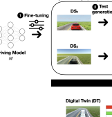
Figure 1: Overview of our approach and its usage.

The goal of our approach is to use digital siblings to test the driving component of an AV. The key intuition is that multiple GPS can better approximate the driving behavior of the AV run in a DT, as opposed to a single-simulator approach. Figure 1 (top) shows an overview of our approach in which two digital siblings, namely DS₁ and DS₂, are used to test the behavior of a driving model under test $M$ (e.g., an end-to-end DNN for lane-keeping).

In the first phase, $M$ is either trained or fine-tuned (step ❶) to run on both DS₁ and DS₂, as well as on the target platform (i.e., DT). A test generation phase (step ❷) is executed for each digital sibling, generating two feature maps $FM_{DS_{1}}$ and $FM_{DS_{2}}$. Feature maps group together test cases with similar feature combination values to reduce redundancy and summarize the AV behavior for unique feature combination deephyperion ; zohdinasabefficient . The value in a feature map cell (displayed in a colored heat scale) represents the average test case outcome, i.e., the behavioral information about the execution of $M$ in each test scenario (e.g., the failure probability). For each simulator, the test generation algorithm produces test scenarios that are executed by $M$ to assess its driving behavior under many different circumstances. Hence, the output of test generation is simulator and model dependent and the feature maps of DS₁ ($FM_{DS_{1}}$) and DS₂ ($FM_{DS_{2}}$) can be different.

The next step of our approach (step ❸) requires to migrate the test cases across simulators. In detail, the test cases in $FM_{DS_{1}}$ are executed on DS₂, resulting in the feature map $\overline{FM}_{DS_{1}}$. Similarly, the test cases in $FM_{DS_{2}}$ are executed on DS₁, resulting in the feature map $\overline{FM}_{DS_{2}}$. Then, for both DS₁ and DS₂, we compute the union of the two feature maps, obtaining $FM_{U_{1}}$ for DS₁ and $FM_{U_{2}}$ for DS₂. Both maps contain the same set of test cases, although executed on two different simulators. The final output of the digital siblings (step ❹) is obtained by merging $FM_{U_{1}}$ and $FM_{U_{2}}$ into the final feature map $FM_{DSS}$.

Step ❺ assesses the correlation of the $FM_{DSS}$ map with the $FM_{DT}$ map, to evaluate the predictive capability of the digital siblings framework. Figure 1 (bottom) shows an overview of the empirical evaluation of our approach (detailed later, in Section 3). All the test cases in the final feature map $FM_{DSS}$ are executed (i.e., migrated) on DT, to obtain the ground truth feature map $FM_{DT}$.

2.1 Test Scenarios

Figure 2: Example of test scenario for a lane-keeping autonomous driving system.

2.1.1 Representation

We adopted an abstract representation of the road in each driving simulator so that only a sequence of road control points is needed when creating a new road in the driving scene. We follow the representation given by Riccio and Tonella deepjanus who defined a two-lane road using a series of control points (displayed as red stars in Figure 2). The control points are interpolated using Catmull-Rom splines 10.1145/378456.378511 , giving the road its final shape (yellow solid line).

Figure 2 shows the visualization of a test scenario generated at step ❷. Specifically, the road is defined using nine control points whereas the Catmull-Rom spline only goes through seven of them. This is because a spline segment (e.g., $P_{2}-P_{3}$) is always defined by four control points (e.g., $P_{1}$, $P_{2}$, $P_{3}$, $P_{4}$). Since two of them are on either side of the endpoints of the spline segment (e.g., $P_{1}$ and $P_{4}$), the spline cannot traverse the extreme endpoints (e.g., $P_{1}$ and $P_{9}$). Hence, $P_{2}$ defines the start point of the road (depicted as a black triangle) whereas $P_{8}$ defines the end point (depicted as a black square).

2.1.2 Implementation

The default initial state of each test case involves positioning the vehicle in the first drivable control point (i.e., $P_{2}$ in Figure 2), at the center of the right lane following the road orientation.

We uniformed the 3D rendering of each simulator such that the driving scenarios have the same look and feel: a two-lane asphalt road, where the road is delimited by two solid white lines on each side and the two driving lanes are separated by a single solid yellow line. The road is placed on top of a green plane representing grass. Harmonization of the driving scenarios across simulators ensures that geometrical features are preserved for the collected driving images and that any color transformation applied to them during training preprocessing remains applicable nvidia-dave2 .

2.1.3 Validity and Oracle

After interpolation, a road is deemed valid if it respects the following constraints: (1) the start and end points are different; (2) the road is contained within a squared bounding box of a predefined size (specifically 250 $\times$ 250); and, (3) there are no intersections.

A test case is deemed successful when the vehicle drives within the right lane until the last road control point (e.g., $P_{8}$ in Figure 2). On the contrary, a test case failure occurs when the vehicle drives out of bound (OOB).

2.2 Creating/Fine-Tuning the Driving Model

For the creation or fine-tuning of a self-driving model (step ❶), a labeled dataset of driving scenes is needed.

2.2.1 Data Collection

We automate labeled data collection by resorting to autopilots that have global knowledge of the driving scenario such as the detailed road geometry and precise vehicle position. In particular, in each simulator, at each step of the simulation, the steering angle of the autopilot is computed by a Proportional-Integral-Differential (PID) controller farag2020complex . The PID controller computes the error between a reference value of a certain variable and its current measured value. Then, it adjusts the controlled system to reach the reference value using three terms, namely Proportional, Integral and Derivative. In the context of self-driving, and in particular in the context of lane-keeping, the error to minimize is the lateral position (LP) which measures the distance between the center of the vehicle and the center of the lane 2020-Stocco-GAUSS (in particular, the lateral position is zero when the vehicle drives at the center of the lane). Given the LP value, the PID controls the steering of the vehicle with the following formula:

$$\textit{steering}=K_{P}\cdot\textsc{LP}+K_{D}\cdot\textit{diff}_{\textsc{LP}}+K_{I}\cdot\textit{total}_{\textsc{LP}}$$ (1)

Equation 1 states that the proportional constant $K_{P}$ acts on the raw error while the derivative constant $K_{D}$ controls the difference between two consecutive errors and the integral constant $K_{I}$ considers the total sum of the errors during the whole simulation until the current timestep. Finally, the steering value is clipped in the interval $[-1,+1]$, where $-1$ means steering all the way to the left and $+1$ to the right ($0$ means the vehicle goes straight as no steering is applied). The steering values are normalized in order to account for the different simulators that we use in our approach.

The autopilot produces a steering angle label for each image which is used to train the driving model. We aligned the frame rates of the different simulators at 20 fps such that each simulator autopilot collects a comparable number of labeled images. The speed of the vehicle, both for the autopilot and $M$, is controlled by the throttle via a linear interpolation between the minimum speed and maximum speed so that the car decreases the speed when the steering angle increases (e.g., in a curve). The following formula computes the throttle based on the speed of the vehicle and the steering:

$$\textit{throttle}=1-\textit{steering}^{2}-\Big{(}\frac{\textit{speed}}{\textit{K}}\Big{)}^{2}$$ (2)

where $K$ is set to a predefined low value $L$ when the measured speed is greater than a given maximum speed threshold, to enforce strong deceleration; viceversa, $K$ is set to a high value $H$ when the measured speed is lower than or equal to the maximum speed threshold, to reduce the deceleration component. From Equation 2, we can see that the throttle is close to 1 (the highest possible value) when the vehicle does not steer ($\textit{steering}=0$) and the speed is substantially lower than the maximum allowed speed (in this case, $K=H$); when one of the two conditions is false the throttle decreases, because of either deceleration component. Similarly to the steering angle values, we clip the throttle value in the interval $[0,1]$.

2.2.2 Model Fine-Tuning via Hybrid Training

The next step involves training the model $M$ using all simulators and the data collected in step ❶. Alternatively, if an existing trained model $M$ is available for the target DT, our approach requires fine-tuning it for all digital siblings. In both scenarios, we use hybrid training based on gradient descent 10.5555/2981562.2981583 .

Hybrid training requires combining the datasets collected for different simulators/platforms into a unified dataset, making sure that each dataset is equally represented (i.e., the unified dataset contains the same number of samples from each simulator/platform specific dataset). Then, the unified dataset is split into training and validation sets (e.g., using the standard 80/20 ratio). The training pipeline is designed in such a way that each image, of dimensions 320$\times$160, is processed according to the simulator/platform it was taken from. For example, images may be cropped differently. Depending on the vehicle size, the front part of the car may, or may not be visible in the frame captured by the camera. Another example of simulator-specific adaptation is the cropping of the above-horizon portion of the image, unnecessary for the lane-keeping task. After cropping, each image is resized to the size required for training, i.e., 320$\times$160.

The training pipeline can be further configured to use plain synthetic virtual images from the driving simulators, or pseudo-real images resembling real-world driving images. The first configuration represents the standard practice in AV testing. In the second configuration, the reality gap due to low photo-realism is reduced by an image-to-image transformation that translates the driving images of each simulator into images similar to those captured by the real-world AV during on-road driving. This practice was proposed in the literature stocco-mind and in industry wayve-sim2real to increase the transferability of the driving model tested in simulation to the real world.

More specifically, this second configuration requires training a CycleGAN model for each driving simulator cyclegan . CycleGAN entails two generators, one that learns how to translate images from simulated to real world (sim2real) and the other that learns the opposite transformation (real2sim). During training of the model, we use the sim2real generator trained for the respective simulator to translate the corresponding training set images. During testing, the sim2real generator translates images on the fly, during the execution of the simulation. We refer to the translated images as pseudo-real, since they are the output of a generative process designed to resemble real images.

Figure 3 shows an example of image translation with a CycleGAN trained for each simulator. The corresponding networks translate an image of a road curve taken in the simulated domain (left) to an image belonging to the real domain (right)—the test track of a small scale physical AV. During training and testing of the driving model in a given simulator, we use the generator of the CycleGAN trained for such simulator.

In our evaluation (Section 3), we consider both configurations of our approach, i.e., training using either simulator or pseudo-real images. We refer to the model trained on simulator images as $M_{S}$, and the model trained on pseudo-real images as $M_{R}$.

Figure 3: Example of translation with the CycleGAN for the three simulators

2.3 Test Generation

While our approach is compatible with any test generation algorithm, in this paper we adopt the MapElites mapelites algorithm implemented in DeepHyperion deephyperion , because the output of DeepHyperion is projected to a feature map that characterizes each generated test scenario according to its features. In other words, test cases having equivalent features (e.g., 3 turns and maximum curvature of 0.2) are grouped into the same cell of the feature map.

Figure 4: Example of feature map generated by DeepHyperion. The two axes represent structural features of the roads.

Figure 4 shows an example of feature map generated by DeepHyperion. The roads (i.e., the test cases) in the map are characterized by two structural features, i.e., the number of turns in the road ($x$ axis) and the curvature of the road ($y$ axis), the latter defined as the minimum radius of the circles going through each sequence of three consecutive road points deephyperion . Such features have been used in previous work and have been shown to be effective at characterizing the search space of road generators deephyperion . Characterizing a test case based on its structural features, i.e., only based on the properties of the road, allows us to identify unique failure scenarios, i.e., failure scenarios with distinctive road properties.

During test generation, the test cases are distributed in the map according to their features. The value of each cell is influenced by the behavior of $M$ when driving on the roads pertaining to a cell. The minimum lateral distance recorded by the simulator is used by DeepHyperion as a fitness of the generated test case. The lateral distance is the opposite of the lateral position, i.e., it is maximum when the vehicle drives at the center of the lane and it decreases as the vehicle approaches the road side. In particular, it is negative when the model misbehaves (i.e., the vehicle goes out of bound). In Figure 4 the two dashed-encircled cells point out two failure cells for $M$ (i.e., cells containing roads with negative fitness).

1

2

3

Input :  $M$, DNN model under test;

  $S$, Simulator instance;

  $P_{s}$, Population size;

  $N$, Number of iterations.

Output :  $F_{m}$, feature map.

4

5$M$ $\leftarrow$ initFeatureMap()

6 $pop$ $\leftarrow$ $\emptyset$

7  /* Generate Initial Population */

8 while $i\leq P_{s}$ do

9       $t_{c}$ $\leftarrow$ generateIndividual()

10       $f$ $\leftarrow$ executeIndividual($t_{c}$, $M$, $S$)

11       placeIndividualMap($F_{m}$, $f$, $t_{c}$)

12       $pop$ $\leftarrow$ $pop$ $\cup$ $\{t_{c}\}$

13 end while

14

15  /* Evolve Individuals */

16 while $i\leq N$ do

17       $t_{c}$ $\leftarrow$ selectIndividual($pop$)

18       $\hat{t}_{c}$ $\leftarrow$ mutateIndividual($t_{c}$)

19       $f$ $\leftarrow$ executeIndividual($\hat{t}_{c}$, $M$, $S$)

20       placeIndividualMap($F_{m}$, $f$, $\hat{t}_{c}$)

21      

22 end while

23

24return $F_{m}$

Algorithm 1 DeepHyperion algorithm

Algorithm 1 shows the pseudocode of the DeepHyperion algorithm. It takes as input the driving model under test $M$, the simulator instance $S$ and two hyperparameters, i.e., the population size $P_{s}$ and the number of iterations $N$ the search is allowed to run, i.e., the budget of the algorithm. The algorithm starts by initializing an empty feature map and population (Lines 1–2). Then, the while loop at Lines 4–9 fills the initial population by randomly generating an individual (Line 5) and executing it to collect its fitness value $f$ (Line 6).

The assignment to the feature map (Line 7) is done by the procedure placeIndividualMap based on the feature values of the individual $t_{c}$ (to determine the coordinates of the target cell) and its fitness value. If the target cell is empty, the individual is placed in the cell. If the cell is non-empty (i.e., another test case was already generated for that cell), a local competition based on the value of the fitness takes place. If the fitness of the individual in the cell is greater than the fitness of the candidate individual, the individual in the cell gets replaced with the candidate individual. Otherwise, no replacement is carried out, which also holds if the individual in the cell already has a negative fitness. The selection function ensures that the search space of the features is explored at large, while the local competition on the individual cells keeps only the lowest performing individuals (i.e., potential misbheaviours) at the end of the generation in order to guide the search towards misbehaviors with unique feature values.

The while loop at Lines 11–16 evolves the initial population of individuals. First, an individual is selected (Line 12) and mutated (Line 13), i.e., the control points of the road are changed in order to form a new individual $\hat{t}_{c}$ with different features. Such individual is then executed (Line 14) and placed in the map (Line 15). The algorithm terminates after a number $N$ of iterations (Line 16).

Algorithm 1 returns a feature map with a single individual for each cell, i.e., the one with the lowest fitness (Line 17). In order to further explore the search space, we run DeepHyperion multiple times for each digital sibling to generate multiple feature maps. Then, we combine such maps by considering the bounds of each feature map axis in all the runs (i.e., minimum and maximum value) and placing each generated individual in the combined map, whose bounds are the lowest (resp. highest) bound values across maps. In this way, there are potentially multiple individuals in each cell and the value of a cell represents the metric of interest averaged over all individuals in that cell (see $FM_{DS_{1}}$ and $FM_{DS_{2}}$ in Figure 1). For instance, considering the failure probability, the value of a cell represents the number of times the model under test failed over the number of all individuals in the cell (a failure occurs when the fitness of an individual is negative).

2.4 Migration and Union

The test generation step produces two feature maps $FM_{DS_{1}}$ and $FM_{DS_{2}}$, for DS₁ and DS₂, respectively. The next step of our approach (i.e., step ❸, see Figure 1) consists of migrating the test cases in $FM_{DS_{1}}$ to DS₂ (producing $\overline{FM}_{DS_{1}}$) and viceversa (producing $\overline{FM}_{DS_{2}}$). Such operation consists of instantiating the abstract (control point based) road representation of the test case being migrated, such that it respects the dimensionality constraints of and it can be supplied as input to the target simulator.

After migration, for both DS₁ and DS₂, we consider the union of their maps. We consider the bounds of each feature in the two maps and we place the respective test cases in a new unified map according to their coordinates, producing the map $FM_{U_{1}}$ for DS₁ (i.e., $FM_{DS_{1}}+\overline{FM}_{DS_{2}}$) and the map $FM_{U_{2}}$ for DS₂ (i.e., $FM_{S_{2}}+\overline{FM}_{S_{1}}$). Hence, the two maps contain the same tests that fill the same cells at the same coordinates.

The value of each cell in the union maps $FM_{U_{1}}$, $FM_{U_{2}}$ is recomputed from the individuals assigned to them. For the failure probability, if a given cell in $FM_{DS_{1}}$ has $n_{1}/N_{1}$ failing individuals, while the corresponding cell in $\overline{FM}_{DS_{2}}$ has $n_{2}/N_{2}$ failing individuals, the failure probability value of the cell in the union map $FM_{U_{1}}$ will be $(n_{1}+n_{2})/(N_{1}+N_{2})$. When a quality of driving metric is computed, instead of a failure probability, the union map will contain the average of the respective quality of driving metrics: $qm=(qm_{1}+qm_{2})/2$, where $qm_{1}$, $qm_{2}$ are the quality of driving metrics found in the same cell in the two feature maps being united ($FM_{DS_{1}},\overline{FM}_{DS_{2}}$, or $FM_{S_{2}},\overline{FM}_{S_{1}}$), while $qm$ is the resulting quality of driving metric, in the union map ($FM_{U_{1}}$ or $FM_{U_{2}}$).

2.5 Merge

The final step of the approach (i.e., step ❹ in Figure 1) requires to merge the two union maps $FM_{U_{1}}$ and $FM_{U_{2}}$ into $FM_{DSS}$. The objective of the merge operation is to combine the testing output of the two digital siblings. Since we aim to use the digital siblings to approximate the behavior of $M$ on DT and predict its failures, the merge operator privileges agreements between the maps of the two digital siblings, i.e., only cells in the maps that have a hot color (e.g., a high failure probability) will produce a hot color in the merged cell. Indeed, such tests are likely to represent simulator-independent misbehaviors of the model under test, which are critical for the safety of the system. Specifically, if the failure probability of $FM_{U_{1}}$ is $fp_{1}=n_{1}/N_{1}$ and that of $FM_{U_{2}}$ is $fp_{2}=n_{2}/N_{2}$, in the merged map the failure probability will be the product, $fp=fp_{1}\times fp_{2}$. When a quality of driving (resp. lack of quality of driving) metric is computed, instead of a failure probability, the merged map will conservatively contain the maximum (resp. minimum) of the respective quality of driving metrics: $qm=\max\{qm_{1},qm_{2}\}$ (resp. $qm=\min\{qm_{1},qm_{2}\}$), where $qm_{1}$, $qm_{2}$ are the quality of driving metrics found in the same cell in $FM_{U_{1}}$, $FM_{U_{2}}$, respectively, while $qm$ is the resulting quality of driving metric, in the merged map. By giving priority to failures (resp. quality of driving degradations) that occur in both siblings and are hence very likely to be relevant for the target platform, this choice better accommodates the limited testing budget available for production/field testing waymo ; borg ; comprehensive-sfc-test ; outsourcing-av-development ; stocco-mind .

2.6 Evaluation Scenario

While our approach is useful when no DT is available, to evaluate whether the DSS can approximate the behavior of $M$ and predict its failures when executed on DT, we migrate all the tests in the digital siblings feature map (i.e., $FM_{DSS}$) to an actual DT, which is used to obtain the ground truth map $FM_{DT}$ (see “Evaluation Scenario” in Figure 1 (bottom)). The two maps being compared contain the same tests in the same cells, but the values of the cells might differ, depending on the behavior of $M$ in the different simulators. Thus, we analyze and compare the two feature maps $FM_{DSS}$ and $FM_{DT}$ to assess the capability of DSS at predicting the failures of the model when executed on the DT.

3 Empirical Study

The goal of the empirical study is to evaluate whether two digital siblings (DSS) can approximate the behavior of a driving model and predict its failures on a digital twin (DT) better than using only one general-purpose simulator (GPS). To this aim, we consider the following research questions:

RQ₁ (Offline Evaluation). How do the offline prediction errors by the DSS compare to those of the DT?

We first test our hypothesis at the model-level. For all simulators, we compute the errors between the model predictions and each autopilot ground truth labels on a stationary driving images dataset. We compare the error distributions of each individual simulator with the DT, as well as their combination as digital siblings.

With RQ₁ we aim to assess whether a correlation between the offline predictions exists at the model-level, which can be useful for developers to gain trust about their DNN model prediction accuracy, prior to running system-level tests.

RQ₂ (Failure Probability). How does the failure probability of the DSS compare to that of the DT?

In RQ₂ we test the model at the system-level, specifically the hypothesis that combining the failure probabilities of the two digital siblings provides a better predictor of the ground truth failure probability of the model executed on the DT. A positive answer to RQ₂ would support our digital siblings framework to predict, and possibly anticipate, the failures on the DT, which are expected to be accurate proxies of real-world failures.

RQ₃ (Quality of Driving). How does the quality of driving of the DSS compare to the failure probability of the DT?

By considering only the failure probability, we might overlook the correlation between real failures on the DT and near-failures on the DSS—test cases in which the model exhibits a degraded driving quality without necessarily going off road. Thus, with RQ₃, we also assess whether finer-grained driving quality metrics can predict the ground truth failure probability of the model on the DT.

3.1 Test Object and Simulators

3.1.1 Study Object

We test a popular DNN-based AV agent: Nvidia DAVE-2 nvidia-dave2 , a robust lane-keeping model used as an object of study in several DNN testing works 2021-Jahangirova-ICST ; 2022-Stocco-ASE ; stocco-mind ; 2020-Stocco-GAUSS ; 2021-Stocco-JSEP ; 2020-Stocco-ICSE ; deephyperion . Moreover, its open-source nature makes it adequate to be trained and evaluated on the simulators considered in this work. Architecturally, DAVE-2 consists of three convolutional layers, followed by five fully-connected layers nvidia-dave2 .

3.1.2 Digital Siblings (DSS)

We implemented and investigated the effectiveness of DSS using the simulators BeamNG beamng and Udacity udacity-simulator . We chose them as digital siblings because: (1) they support training and testing of a DNN that performs lane-keeping, including DAVE-2; (2) they are often used as simulator platforms for AV testing; (3) they are potentially complementary because they are developed with different technologies/game engines and they are characterized by different physics implementations (e.g., rigid vs soft-body dynamics); (4) they are publicly available under open-source or academic-oriented licenses, hence customizable.

BeamNG beamng is a framework specialized in autonomous driving developed by BeamNG GmbH. The framework is released under an academic-oriented license and it has been downloaded 5.5$k$ times as of January 2023. From a technical standpoint, BeamNG features a soft-body dynamics simulation based on a spring-mass model. Such a model is composed of nodes (mass points) that are connected by beams (springs), i.e., weightless elements that allow accurate vehicle deformation and other aerodynamic properties gambi-beamng .

Udacity udacity-simulator is developed with Unity 3D unity , a popular cross-platform game engine. The project has been publicly released in 2016 by the for-profit educational organization Udacity, to allow people from all over the world to access some of their technology and to contribute to an open-source self-driving car project. As of January 2023, the simulator has 3.7$k$ stars on GitHub. From a technical standpoint, Udacity is based on the Nvidia PhysX engine PhysX , featuring discrete and continuous collision detection, ray-casting, and rigid-body dynamics simulation.

3.1.3 Digital Twin (DT)

We use the Donkey Car^™ open-source framework donkeycar as digital twin for our study. This platform has been used for AV testing research with physical self-driving cars in physical environments stocco-mind ; viitala ; 9412011 . The framework includes open hardware to build 1:16 scale radio-controlled cars with self-driving capabilities, a Python framework for training and testing DNN models with lane-keeping functionalities using supervised or reinforcement learning, and a simulator in which the real-world Donkey Car is faithfully modeled. This was assessed by a recent work stocco-mind reporting that, for three lane-keeping models, the steering angle distribution of the AV model driving in the real-world environment is statistically indistinguishable from the steering angle distribution of the AV model driving in the digital twin.

In the rest of the section, we refer to BeamNG as DS₁, Udacity as DS₂, the combined digital siblings as DSS, and DonkeyCar as DT.

3.2 Procedure

3.2.1 CycleGAN Models

Data Collection. We collected 15k simulated images, 5k for DS₁ and DS₂ by running the autopilots on a set of randomly generated roads. Moreover, we collected 5k real-world images stocco-mind by manually driving the physical twin of the DT on a physical road track in our lab.

Training. We trained three CycleGAN models, one for each simulator, with the obtained training sets (5k virtual images and 5k real-world images). Each model was trained for 60 epochs using the default hyper-parameters of the original paper cyclegan . We saved a checkpoint model every 5 epochs and we ultimately chose the one that achieved the best neural translations (in terms of visual quality) using a test set of $\approx$8k simulated images for each simulator, representing a test road driven from beginning to the end stocco-mind . While a quantitative assessment of the output of CycleGAN is still a major challenge pros-and-cons-gans and out of the scope of this paper, the driving capability of the lane-keeping model, as the experimental evaluation shows, represents an implicit validation of the CycleGAN model’s ability to retain all essential features needed for an accurate steering angle prediction.

3.2.2 Driving Models

Data Collection. For all simulators (i.e., DS₁, DS₂ and DT), we collected a training set by running the autopilots on a set of randomly generated roads (this set is different from the one used to train the CycleGAN). To ensure having non-trivial driving scenarios and appropriate labels for challenging curves, the maximum angle of a curve was set to be less than or equal to $270^{\circ}$. In particular, for our training set, we generated 25 roads with 8 control points deephyperion . To collect a balanced dataset where left and right curves are equally represented, each road was driven by the autopilot in both directions, i.e., from the start point to the end point and from the end point to the start point. The autopilot drove successfully the totality of the roads on all simulators; our training set comprises $\approx$70k images, equally distributed across the simulators.

Training. We trained two DAVE-2 models, one by using the plain simulated images ($M_{S}$) and another one by translating the images of each simulator into pseudo-real images ($M_{R}$) using the respective CycleGAN generator. We followed the guidelines by Bojarski et al. nvidia-dave2 to train AV autopilots. For both $M_{S}$ and $M_{R}$ we trained the model for 50 epochs, with an early stopping patience of 10 epochs if no improvements of the validation loss were observed during fitting. We used the Adam optimizer kingma2014adam to minimize the mean squared error (MSE) between the predicted steering angles and the ground truth value. Moreover, we set a learning rate of $10^{-4}$ and a batch size of 128. The best MSE on the validation set for $M_{S}$ was 0.003, reached after 48 epochs, whereas the best MSE on the validation set for $M_{R}$ was 0.02, reached after 25 epochs.

3.2.3 Offline Evaluation

We collected a labeled dataset for offline evaluation by generating 20 roads (i.e., 10 roads driven in both directions) with the same parameters as the training set (i.e., 8 control points per road and a maximum angle of $270^{\circ}$). The images collected for the offline evaluation dataset amount to $\approx$26k, considering all simulators.

3.2.4 Test Generation

After training $M_{S}$ and $M_{R}$, we executed DeepHyperion twice to generate tests using the two digital siblings DS₁ and DS₂. We chose a population size of 20 individuals and a number of search iterations respectively equal to 150 for $M_{S}$ and 100 for $M_{R}$, as we observed from preliminary experiments that this choice of hyper-parameters allows an extensive coverage of the feature maps. For both $M_{S}$ and $M_{R}$ and each digital sibling, we repeated test generation five times to diversify the exploration of the search space and to collect multiple test cases for each cell in the feature maps. Overall, across all runs and driving models, DeepHyperion generated 1,455 tests for both siblings.

Concerning the simulations, for all simulators, we set the maximum speed for the vehicle to 30 km/h deephyperion . When testing $M_{R}$ in a given simulator, we engineered the testing pipeline to load the appropriate sim2real CycleGAN generator to translate the simulated image generated by BeamNG/Udacity into pseudo-real images in real-time during driving. For each executed test case, we collected the lateral position of the vehicle for each simulation step as well as its lateral distance. The former determines the quality of driving of the model 2021-Jahangirova-ICST , while the latter is the fitness of the test case.

3.2.5 Migration and Union

For the initial ($FM_{DS_{1}}$, $FM_{DS_{2}}$) and for the union ($FM_{U_{1}}$, $FM_{U_{2}}$) feature maps, we compute the failure probability as the number of tests with a negative fitness divided by the total number of tests in the respective cell. To evaluate the quality of driving, we adopted the maximum lateral position experienced during the test case execution. Previous work showed that such metric is effective at characterizing the degradation in the quality of autonomous driving 2021-Jahangirova-ICST since the lower the value of such metric, the higher is the quality of driving (thus, it actually measures lack of quality of driving). When considering the quality of driving, the value of each cell in a feature map represents the average of the maximum lateral positions of each test case in that cell. Furthermore, we normalized the maximum lateral position values in the interval $[0,1]$ before taking the union.

3.2.6 Merge

Merging the maps of the two digital siblings requires a different treatment for failure probability and quality of driving. Regarding the failure probability, the merge operator that ensures a conservative aggregation of two values is the product. Regarding the lack of quality of driving, the conservative merge operator is the minimum, since the quantities to merge are not probabilities. In fact, by taking the minimum we get a high lack of driving quality only when both simulators exhibit high values for such a metric.

3.3 Metrics

3.3.1 RQ₁ (Offline Evaluation)

We computed the prediction errors given by the difference between the predictions of the model ($M_{R}$) on images of the offline evaluation dataset (see Section 3.2) and the corresponding ground truth labels given by the autopilot. We binned the prediction errors of the model on each simulator and built the respective probability density (i.e., the number of errors in each bin is divided by the total number of prediction errors) such that different distributions could be compared.

Then, we computed the distance between each digital sibling distribution, as well as their combination, and the DT using the Wasserstein distance wgan (also known as the earth mover’s distance). Given two one-dimensional distributions $A$ and $B$, the Wasserstein distance $W(A,B)$ is defined by the following formula wasserstein :

$$W(A,B)=\int_{\mathbb{R}}|CDF_{A}(x)-CDF_{B}(x)|dx$$ (3)

where $CDF$ is the cumulative distribution function of a distribution. In other words, the Wasserstein distance between two distributions is defined as the difference between the area formed by their cumulative distribution functions.

We assess whether the difference between two distributions is statistically significant using the Wilcoxon test non-parametric-book applied to the density functions of the two error distributions to compute the $p$-value (with threshold $\alpha\leq 0.05$). We also perform power analysis (with statistical power $\beta\geq 0.8$) on the prediction errors to check whether a non-significant $p$-value is due to a low data sample size or to the difference being statistically insignificant.

3.3.2 RQ₂ (Failure Probability) and RQ₃ (Quality of Driving)

For RQ₂, we computed the pairwise Pearson correlation between maps along with the corresponding $p$-value. In particular, correlations are computed between each union feature map of each digital sibling ($FM_{U_{1}}$, $FM_{U_{2}}$) and the feature map of the DT ($FM_{DT}$), and between $FM_{DSS}$ and $FM_{DT}$. For RQ₃, the setting is equivalent to that of the failure probability but considering quality of driving maps, again comparing DS₁, DS₂ and DSS against the ground truth DT.

To evaluate the capabilities of the digital siblings (individually or jointly) to predict failures on the DT, we computed the area under the curve Precision-Recall (AUC-PRC) at increasing thresholds, for both RQ₂ and RQ₃. This requires the discretization of failure probabilities into binary values (failure vs non-failure) for the ground truth (i.e., DT): we consider a cell in the DT feature map to be a failure cell if the associated failure probability is $>0.0$. AUC-PRC is more informative than the AUC-ROC metric (i.e., the area under of the curve of the Receiver Operating Characteristics) when dealing with imbalanced prc-justification datasets, which is the case of our study (the number of failures in the feature maps is lower than the number of non-failures with an average 10 to 20% ratio).

[b]

Table 1: Results for RQ₁. Bold-faced values indicate the best approach.

	Offline Evaluation
	$M_{S}$		$M_{R}$
	distance	$p$-value	distance	$p$-value
DS1 vs DT	0.04669	0.101$\dagger$	0.03250	0.011
DS2 vs DT	0.02648	0.020	0.02187	0.078$\dagger$
DSS vs DT	0.03776	0.053$\dagger$	0.00951	0.088$\dagger$

• power $>$ 0.8

3.4 Results

3.4.1 Offline Evaluation (RQ₁)

Table 1 reports the results for our first research question. The first column shows the simulators being compared. Columns 2–5 report the Wasserstein distance between the prediction error densities of the corresponding simulators, and the $p$-value concerning the statistical significance of the differences between the two densities, for $M_{S}$ and $M_{R}$.

For $M_{S}$ (Columns 2–3), our results show that the distance between the steering angle errors obtained for the combined digital siblings DSS and the errors obtained for the DT is lower than the distance of DS₁ (0.03776 vs 0.046) and higher than the distance of DS₂ (0.02648). The distribution of the steering angle errors of DS₂ is statistically different from the errors of the DT (i.e., $p$-value 0.02 $<0.05$), while the distribution of the steering angle errors of DSS is statistically indistinguishable from the errors of the DT (i.e., $p$-value 0.053 $>0.05$ and power $>0.8$).

Regarding $M_{R}$ (Columns 4–5), our results show that the distance between the steering angle errors obtained for the combined digital siblings DSS and the errors obtained for the DT is 2.8 times lower than the distance of each simulator taken individually (as a percentage, the distance of DSS is respectively 70% and 56% smaller than the distance of the two individual siblings, DS₁, DS₂). The statistical test confirms that the error distributions of DSS and DT are statistically indistinguishable ($p$-value $>$ 0.05 and power $>$ 0.8), which is not the case for the error distributions of DS₁ ($p$-value $<$ 0.05).

Figure 5 offers a visual explanation of these scores. The subplots compare the steering angle error distributions, respectively, of DS₁, DS₂ and DSS (shown in light red) with that of DT (shown in light blue). The $x$-axis of each subplot represents the magnitude of the prediction errors of the model $M_{R}$ w.r.t. the predictions of the autopilot, while the $y$-axis indicates their percentage for each bin.

Figure 5: Distributions of prediction errors of $M_{R}$ in the two digital siblings, i.e., DS₁ and DS₂, their combination (DSS) and the DT. Best viewed in color.

From the plots we can see that, overall, at the model-level, $M_{R}$ makes prediction errors with small magnitudes on DS₁, DS₂ and DSS (i.e., most of the errors are between 0.0 and 0.3). On the digital sibling DS₁ (i.e., BeamNG), $M_{R}$ has a high agreement with the autopilot, as most errors have a low magnitude. It has a large number of small errors ($<0.2$), while it has only a negligible portion of the distribution being above 0.2. The agreement with the DT is low as $M_{R}$ under-approximates the true error distribution on the DT: $M_{R}$ on the DT has less errors with low magnitude and has a longer tail of errors greater than 0.2 (even greater than 0.3 in some cases). Differently, on the digital sibling DS₂ (i.e., Udacity), the error distribution has a longer tail than that on the DT. Indeed, $M_{R}$ executed on DS₂ over-approximates the errors it would have on the DT, as the errors observed on DS₂ have higher magnitude than those observed on the DT.

The error distribution of the model on DSS shows why it is appropriate to combine the outcome of two simulators. At the model-level, DSS better approximates the true error distribution of the model on the DT, by providing an intermediate error between DS₁ and DS₂ for both $M_{S}$ and $M_{R}$.

3.4.2 Failure Probability (RQ₂)

Table 2 shows the Pearson correlation (r), the $p$-value, and the AUC-PRC for the comparison between DS₁, DS₂, DSS and DT, respectively. The analysis is reported separately for $M_{S}$ (Columns 2–4) and $M_{R}$ (Columns 5–7).

Table 2: Results for RQ₂. Bold-faced values indicate the best approach.

	Failure Probability
	$M_{S}$			$M_{R}$
	r	$p$-value	AUC-PRC	r	$p$-value	AUC-PRC
DS1 vs DT	0.650	0.000	0.654	0.194	0.087	0.395
DS2 vs DT	0.583	0.000	0.512	0.077	0.499	0.328
DSS vs DT	0.710	0.000	0.684	0.193	0.088	0.400

Concerning $M_{S}$—i.e., the model driving with simulated driving scenes— the failure probabilities have a high positive correlation with the true failure probability of the DT (Column 2). All such correlations are statistically significant for our DSS framework, as well as for each individual sibling DS₁ and DS₂ ($p$-values $<$ 0.05, see Column 3).

Figure 6: Feature maps representing the failure probability of $M_{S}$ on the two digital siblings, DS₁ and DS₂, their combination (DSS) and on the DT. Solid line cells represent a true failure predicted by DSS while dashed line cells represent a false positive of DS₂. Best viewed in color.

However, the correlation of the DSS is 9% higher than the best individual correlation (i.e., DS₁) and 21% higher than the worst individual correlation (i.e., DS₂). In terms of failure prediction, the DSS have the highest AUC-PRC value, 4% higher than DS₁ and 33% higher than DS₂.

Figure 6 shows the feature maps related to $M_{S}$. The first three feature maps represent the failure probability of DS₁, DS₂ and DSS, respectively. The last feature map represents the ground truth failure probability of DT. The color of each cell ranges from green (i.e., non-failure, or failure probability = 0) to red (i.e., failure probability = 1). Let us analyze a false positive case. The test cases at coordinates (3, 0.25), whose corresponding cells are highlighted with a dashed line, represent road tracks having three curves and a maximum curvature of 0.25. In the DT, this cell is green, i.e., all test cases for $M_{S}$ driving on the DT succeed. On the other hand, $M_{S}$ has contrasting behaviors when the same test cases are executed on DS₁ or DS₂. These test cases did not exhibit any failure in DS₁, whereas they did trigger failures in DS₂. This disagreement is canceled out when combining the two digital siblings with the product operator and the cell is green in the DSS map. As such, digital siblings are conservative w.r.t. failures, as a failure is reported only when both digital siblings are in agreement. This can be noticed for test cases at coordinates (1, 0.23), which represent road tracks having one curve with a maximum curvature of 0.23—an instance of a true positive case (the corresponding cells in each map are highlighted with a solid line). Both DS₁ and DS₂ have a failure probability of 1 and, as a consequence, the DSS map also does. On the DT, $M_{S}$ has also a high failure probability (0.5), which confirms the high effectiveness of the DSS framework at approximating the true failure probability of DT.

Concerning the failure probability for $M_{R}$—i.e., the model driving with pseudo-real driving scenes, the correlation of the DSS is comparable with the best individual correlation (i.e., 0.193 for DSS vs 0.194 for DS₁). Similarly, the corresponding AUC-PRC values are equivalent (the AUC-PRC of DSS is 1% better than that of DS₁). All correlations are not statistically significant; especially the correlation of DS₂ with the DT is particularly low (i.e., 0.077), which is also reflected in the low AUC-PRC score (i.e., 0.328). In this case the usage of the DSS framework mitigates (actually, eliminates) the risk of choosing a poorly performing simulator such as DS₂, which exhibits low correlation of the failure probability with the ground truth one and low failure prediction power.

3.4.3 Quality of Driving (RQ₃)

Table 3 shows the Pearson correlation (r), the $p$-value, and the AUC-PRC for the comparison between DS₁, DS₂, DSS and DT, respectively. The comparison considers the correlation between the quality of driving metric experienced in DS₁, DS₂, DSS and the failure probability of the model on the DT, as well as the prediction of failures from the quality of driving metric. The analysis is reported separately for both $M_{S}$ (Columns 2–4) and $M_{R}$ (Columns 5–7) models.

For $M_{S}$, the correlation between DSS and DT is lower than the best individual correlation (0.553 of DSS vs 0.621 of DS₁). The DSS correlation is 22% higher than the worst individual correlation (0.553 of DSS vs 0.429 of DS₂). For AUC-PRC, DSS and DS₂ have the same predictive power (i.e., 0.659), while DSS is 25% better than DS₂ (i.e., 0.659 vs 0.496). Thus, using the DSS framework mitigates the risk of relying on the testing results of a low-quality GPS (i.e., DS₂).

Concerning $M_{R}$, we observed a similar correlation and a similar AUC-PRC as with $M_{S}$, the main difference being the slightly higher AUC-PRC for DSS (i.e., 0.500 vs 0.490) w.r.t. the best individual sibling (i.e., DS₁) and a more pronounced difference w.r.t. the worst individual sibling (i.e., DS₂, 0.659 vs 0.496 in $M_{S}$, a 33% increase, and 0.500 vs 0.336 in $M_{R}$, a 49% increase).

Figure 7 shows the four feature maps related to the quality of driving of the $M_{R}$ model on the two digital siblings and the failure probability of $M_{R}$ on the DT. We can observe that the feature map of DS₁ and the feature map of the DSS are similar. As a consequence, the two correlations are similar. On the other hand, the feature map of DS₂ is quite different from the failure probability map of the DT, which causes the correlation to be low. We can observe that a failure case of the DT at coordinates (1, 0.14) is not caught by the quality metric values of any sibling (neither DS₁, DS₂, nor DSS, see the corresponding cells highlighted with a solid line). On the other hand, all siblings are able to capture the failure of the DT at coordinates (3, 0.23) (see the corresponding cells highlighted with a dashed line).

Table 3: Results for RQ₃. Bold-faced values indicate the best approach.

	Quality of Driving
	$M_{S}$			$M_{R}$
	r	$p$-value	AUC-PRC	r	$p$-value	AUC-PRC
DS1 vs DT	0.621	0.000	0.659	0.211	0.062	0.490
DS2 vs DT	0.429	0.000	0.496	0.056	0.626	0.336
DSS vs DT	0.553	0.000	0.659	0.193	0.088	0.500

Figure 7: Feature maps representing the quality of driving of $M_{R}$ (i.e., the maximum lateral position) on the two digital siblings, DS₁ and DS₂, their combination (DSS) and the failure probability on the DT. Solid line cells represent a true failure missed by all siblings, while dashed line cells represent a true failure predicted by DSS. Best viewed in color.

4 Discussion

When combining the two siblings using our framework, the worst case occurs when the two siblings disagree and the over-approximating sibling (e.g., predicting a failure) is not compensated by the under-approximating sibling (see Figure 6). In practical cases, we empirically observed that by predicting a failure only when there is agreement, the digital siblings framework is equivalent to the best of the two siblings (see RQ₃).

We experimented with both simulated ($M_{S}$) and real-world models ($M_{R}$) as such setting is representative of the current industrial testing practices described by the NHTSA nhtsa . From the feature maps in Figure 6 and Figure 7, we can observe that the driving quality of $M_{S}$ is superior w.r.t. $M_{R}$, presumably because it is easier for a DNN to process plain artificial images from a simulator, rather than the images collected by a real-world camera during driving (i.e., sim2real gap). Our results show that, in both settings, using the digital siblings better approximates the behavior of the model on the DT, regardless of the different driving capabilities.

4.1 Threats to Validity

4.1.1 Internal validity

We compared all simulators under identical parameter settings. One threat to internal validity concerns our custom implementation of DeepHyperion within the simulators. We mitigated this threat by faithfully replicating the code available in the replication package of the paper deephyperion-tool . Another threat may be due to our own data collection phase and training of DAVE-2, which may exhibit a large number of misbehaviors if trained inadequately. We mitigated this threat by training and fine-tuning a model which was able to drive on the training set roads consistently on all simulators.

4.1.2 External validity

We considered only a limited number of DNN models and simulators, which poses a threat in terms of the generalizability of our results. We tried to mitigate this threat by choosing a popular real-world DNN model, which achieved competitive scores in the Udacity challenge. We considered two open-source GPS and we chose DonkeyCar as DT, as it was used as a proxy for full size self-driving cars also in previous studies stocco-mind ; 2021-01-0248 ; viitala ; 9412011 . Generalizability to other GPS or DT would require further studies.

5 Related Work

5.1 Digital Twins for AV Testing

Digital twins are used by researchers to reproduce real-world conditions within a simulation environment for testing purposes 10.1007/978-3-030-59155-7_39 ; 9369807 ; DBLP:journals/corr/abs-2012-05841 ; san2021digital ; 9392784 .

Yun et al. 9369807 test an object recognition system using the GTA videogame. Barosan et al. 10.1007/978-3-030-59155-7_39 describe a digital twin for testing an autonomous truck. No testing was performed using the digital twin to assess the faithfulness of the simulator at reproducing real-world failures.

Differently, in our paper we investigate testing transferability between digital siblings, i.e., a framework composed of multiple general-purpose simulators, and a digital twin, considering both simulated and pseudo-real images as input to the DNN.

5.2 Empirical Studies

Recent work has confirmed the need for real-world testing of cyber-physical systems, as simulation platforms are often decoupled from the real world complexities icst-survey-robotics . Our work is the first to propose the usage of a multi-simulator approach, called digital siblings, to mitigate the fidelity gap in the field of autonomous driving testing.

Concerning comparative studies across simulators, to the best of our knowledge, the only study that empirically compares the same AV on different simulation platforms is by Borg et al. borg . The authors investigate the use of multiple GPS for testing a pedestrian vision detection system. The study compares a large set of test scenarios on both PreScan prescan and Pro-SiVIC pro-sivic and reports low agreement between testing results across the two simulation platforms. No assessment is performed of their correlation with a digital twin or a physical vehicle. In our paper, we take a step ahead and we show how the (dis)agreements can be leveraged to mitigate the fidelity gap: by combining the predictions of two general-purpose simulators we successfully covered the gap with a digital twin for a scaled physical vehicle.

Other studies compare model-level vs system-level testing metrics within a simulation environment briand-offline-emse . In our empirical work, we focused on the difference between general-purpose and digital twin driving simulators. We use offline and online testing to measure the gap between single- and multi-simulator approaches at approximating a digital twin, a previously unexplored topic.

5.3 AV Testing Approaches

Most approaches use model-level testing (i.e., offline testing of single image predictions) to test DNN autopilots under corrupted images deeptest or GAN-generated driving scenarios deeproad , without however testing the self-driving software in its operational domain. In our work, we assess the effectiveness of our digital siblings with model-level testing in terms of prediction error distributions, but we also consider online testing at the system-level.

Concerning system-level testing for AVs, researchers proposed techniques to generate scenarios that cause AVs to misbehave 2020-Stocco-ICSE ; asfault ; 2021-Stocco-JSEP ; 2022-Stocco-ASE ; arxiv.2203.12026 ; deeproad . Among the existing test generators, in this work we adopted DeepHyperion by Zohdinasab et al. deephyperion , a tool that uses illumination search to extensively cover a map of structural input features, which allowed us to easily group identical or equivalent failure conditions occurring in the same feature map cell. Ul Haq et al. DBLP:conf/icse/Haq0B22 use ML regressors as surrogate models to mimic the simulator’s outcome.

These works only consider single-simulator approaches to testing. Their generalizability to a multi-simulator approach, such as the digital siblings proposed in this paper, or to cross-simulator testing, is overlooked in the existing literature.

6 Conclusions and Future Work

In this paper, we propose the digital siblings framework to improve the testing of autonomous driving software. In our approach, we test the autonomous driving software using two general-purpose simulators in order to better approximate the behavior of the driving model on a digital twin. We combine the testing outputs of the model on the two simulators in a conservative way, giving priority to the agreements on possible failures, where it is more likely to observe the same failing behavior on the digital twin.

At the model level, our results show that, by combining two general-purpose simulators, we can approximate the model predictions on the digital twin better than done by each individual simulator. At the system-level, the digital siblings are able to predict the failures of the model on the digital twin better than each single simulator.

In our future work we plan to extend our framework to more than two general-purpose simulators and to study different ways to combine them based on the characteristics of each simulator and those of the digital twin.

7 Declarations

7.1 Funding and/or Conflicts of interests/Competing interests

This work was partially supported by the H2020 project PRECRIME, funded under the ERC Advanced Grant 2017 Program (ERC Grant Agreement n. 787703). We thank BeamNG GmbH for providing us the license for the driving simulator. The authors declared that they have no conflict of interest.

7.2 Data Availability

The software artifacts and our results are publicly available tool .

References

- (1) Afzal, A., Katz, D.S., Le Goues, C., Timperley, C.S.: Simulation for robotics test automation: Developer perspectives. In: 2021 14th IEEE Conference on Software Testing, Verification and Validation (ICST), pp. 263–274. IEEE (2021)
- (2) Almeaibed, S., Al-Rubaye, S., Tsourdos, A., Avdelidis, N.P.: Digital twin analysis to promote safety and security in autonomous vehicles. IEEE Communications Standards Magazine 5(1), 40–46 (2021). DOI 10.1109/MCOMSTD.011.2100004
- (3) Arjovsky, M., Chintala, S., Bottou, L.: Wasserstein generative adversarial networks. In: International conference on machine learning, pp. 214–223. PMLR (2017)
- (4) Barosan, I., Basmenj, A.A., Chouhan, S.G.R., Manrique, D.: Development of a virtual simulation environment and a digital twin of an autonomous driving truck for a distribution center. In: Software Architecture, pp. 542–557. Springer, Cham (2020)
- (5) Barry, P.J., Goldman, R.N.: A recursive evaluation algorithm for a class of catmull-rom splines. SIGGRAPH Comput. Graph. (1988)
- (6) BeamNG.research: BeamNG GmbH. https://www.beamng.gmbh/research (2022)
- (7) Bewley, A., Rigley, J., Liu, Y., Hawke, J., Shen, R., Lam, V.D., Kendall, A.: Learning to drive from simulation without real world labels. In: 2019 International conference on robotics and automation (ICRA), pp. 4818–4824. IEEE (2019)
- (8) BGR Media, L.: Waymo’s self-driving cars hit 10 million miles. https://techcrunch.com/2018/10/10/waymos-self-driving-cars-hit-10-million-miles (2018)
- (9) Bojarski, M., Del Testa, D., Dworakowski, D., Firner, B., Flepp, B., Goyal, P., Jackel, L.D., Monfort, M., Muller, U., Zhang, J., Zhang, X., Zhao, J., Zieba, K.: End to end learning for self-driving cars. CoRR abs/1604.07316 (2016)
- (10) Borg, M., Abdessalem, R.B., Nejati, S., Jegeden, F.X., Shin, D.: Digital twins are not monozygotic–cross-replicating adas testing in two industry-grade automotive simulators. In: ICST ’21. IEEE (2021)
- (11) Borji, A.: Pros and cons of gan evaluation measures. Computer Vision and Image Understanding 179, 41–65 (2019)
- (12) Bottou, L., Bousquet, O.: The tradeoffs of large scale learning. In: Proceedings of NIPS ’07 (2007)
- (13) Boutan, E.: Autonomous driving market overview. https://medium.com/swlh/autonomous-driving-market-overview-b8c71d81c072 (2020)
- (14) Cerf, V.G.: A comprehensive self-driving car test. Communications of the ACM 61(2) (2018)
- (15) Conover, W.J.: Practical nonparametric statistics, vol. 350. john wiley & sons (1999)
- (16) DeepHyperion Replication package. https://github.com/testingautomated-usi/DeepHyperion (2022)
- (17) Donkey Car. https://www.donkeycar.com/ (2021)
- (18) Farag, W.: Complex trajectory tracking using pid control for autonomous driving. International Journal of Intelligent Transportation Systems Research 18(2), 356–366 (2020)
- (19) Gambi, A., Maul, P., Mueller, M., Stamatogiannakis, L., Fischer, T., Panichella, S.: Soft-body simulation and procedural generation for the development and testing of cyber-physical systems. Tech. rep., BeamNG (2019)
- (20) Gambi, A., Mueller, M., Fraser, G.: Automatically testing self-driving cars with search-based procedural content generation. In: Proceedings of ISSTA ’19 (2019)
- (21) García, S., Strüber, D., Brugali, D., Berger, T., Pelliccione, P.: Robotics software engineering: A perspective from the service robotics domain. In: Proceedings of ESEC/FSE ’20, pp. 593–604 (2020)
- (22) Grigorescu, S., Trasnea, B., Cocias, T., Macesanu, G.: A survey of deep learning techniques for autonomous driving. Journal of Field Robotics 37(3), 362–386 (2020)
- (23) Group, E.: Esi prosivic. https://myesi.esi-group.com/downloads/software-downloads/pro-sivic-2021.0 (2021)
- (24) Haq, F.U., Shin, D., Briand, L.C.: Efficient online testing for dnn-enabled systems using surrogate-assisted and many-objective optimization. In: 44th IEEE/ACM 44th International Conference on Software Engineering, ICSE 2022, USA, pp. 811–822. ACM (2022)
- (25) Haq, F.U., Shin, D., Nejati, S., Briand, L.: Can offline testing of deep neural networks replace their online testing? Empirical Software Engineering (2021)
- (26) Jahangirova, G., Stocco, A., Tonella, P.: Quality metrics and oracles for autonomous vehicles testing. In: Proceedings of 14th IEEE International Conference on Software Testing, Verification and Validation, ICST ’21. IEEE (2021)
- (27) Kapteyn, M.G., Pretorius, J.V.R., Willcox, K.E.: A probabilistic graphical model foundation for enabling predictive digital twins at scale. CoRR abs/2012.05841 (2020)
- (28) Kaur, P., Taghavi, S., Tian, Z., Shi, W.: A survey on simulators for testing self-driving cars. CoRR abs/2101.05337 (2021). URL https://arxiv.org/abs/2101.05337
- (29) Kingma, D.P., Ba, J.: Adam: A method for stochastic optimization. arXiv preprint arXiv:1412.6980 (2014)
- (30) Koopman, P., Wagner, M.: Challenges in autonomous vehicle testing and validation. SAE International Journal of Transportation Safety (2016)
- (31) Kothlow, C.: The power of a multi-purpose digital twin. https://blogs.sw.siemens.com/simcenter/the-power-of-a-multi-purpose-digital-twin/ (2021)
- (32) May, C.: Why automotive companies outsource software development services. https://medium.datadriveninvestor.com/why-automotive-companies-outsource-software-development-services-54a806458b4?gi=9d9b4f45e9ba (2019)
- (33) Moghadam, M.H., Borg, M., Saadatmand, M., Mousavirad, S.J., Bohlin, M., Lisper, B.: Machine learning testing in an adas case study using simulation-integrated bio-inspired search-based testing (2022)
- (34) Mouret, J.B., Clune, J.: Illuminating search spaces by mapping elites. arXiv preprint arXiv:1504.04909 (2015)
- (35) Nvidia PhysX. https://developer.nvidia.com/physx-sdk (2022)
- (36) Ramdas, A., García Trillos, N., Cuturi, M.: On wasserstein two-sample testing and related families of nonparametric tests. Entropy 19(2), 47 (2017)
- (37) Replication package. https://github.com/testingautomated-usi/maxitwo (2023)
- (38) Riccio, V., Tonella, P.: Model-based exploration of the frontier of behaviours for deep learning system testing. In: Proceedings of ESEC/FSE (2020)
- (39) Rosique, F., Navarro, P.J., Fernández, C., Padilla, A.: A systematic review of perception system and simulators for autonomous vehicles research. Sensors 19(3) (2019). DOI 10.3390/s19030648
- (40) Saito, T., Rehmsmeier, M.: The precision-recall plot is more informative than the roc plot when evaluating binary classifiers on imbalanced datasets. PloS one 10(3), e0118,432 (2015)
- (41) San, O.: The digital twin revolution. Nature Computational Science 1(5), 307–308 (2021)
- (42) Software, S.D.I.: Simcenter prescan. https://www.plm.automation.siemens.com/global/en/products/simcenter/prescan.html (2022)
- (43) Stocco, A., Nunes, P.J., d’Amorim, M., Tonella, P.: Thirdeye: Attention maps for safe autonomous driving systems. In: Proceedings of 37th IEEE/ACM International Conference on Automated Software Engineering, ASE ’22. IEEE/ACM (2022)
- (44) Stocco, A., Pulfer, B., Tonella, P.: Mind the Gap! A Study on the Transferability of Virtual vs Physical-world Testing of Autonomous Driving Systems. IEEE Transactions on Software Engineering (2022). URL https://ieeexplore.ieee.org/document/9869302
- (45) Stocco, A., Tonella, P.: Towards anomaly detectors that learn continuously. In: Proceedings of 31st International Symposium on Software Reliability Engineering Workshops, ISSREW 2020. IEEE (2020)
- (46) Stocco, A., Tonella, P.: Confidence-driven weighted retraining for predicting safety-critical failures in autonomous driving systems. Journal of Software: Evolution and Process (2021). DOI 10.1002/smr.2386
- (47) Stocco, A., Weiss, M., Calzana, M., Tonella, P.: Misbehaviour prediction for autonomous driving systems. In: Proceedings of 42nd International Conference on Software Engineering, ICSE ’20. ACM (2020)
- (48) Tang, S., Zhang, Z., Zhang, Y., Zhou, J., Guo, Y., Liu, S., Guo, S., Li, Y., Ma, L., Xue, Y., Liu, Y.: A survey on automated driving system testing: Landscapes and trends. CoRR abs/2206.05961 (2022). DOI 10.48550/arXiv.2206.05961. URL https://doi.org/10.48550/arXiv.2206.05961
- (49) Tawn Kramer, M.E., contributors: Donkeycar. https://www.donkeycar.com/ (2022)
- (50) Team, U.: Udacity’s self-driving car simulator. https://github.com/tsigalko18/self-driving-car-sim (2019)
- (51) Tian, Y., Pei, K., Jana, S., Ray, B.: Deeptest: Automated testing of deep-neural-network-driven autonomous cars. In: Proceedings of ICSE ’18. ACM (2018)
- (52) of Transportation, U.D.: A framework for automated driving system testable cases and scenarios. https://rosap.ntl.bts.gov/view/dot/38824/dot_38824_DS1.pdf (2018)
- (53) Udacity: A self-driving car simulator built with Unity. https://github.com/udacity/self-driving-car-sim (2017). Online; accessed 18 August 2019
- (54) Unity3d. https://unity.com (2021)
- (55) van Dinter, R., Tekinerdogan, B., Catal, C.: Predictive maintenance using digital twins: A systematic literature review. Information and Software Technology (2022)
- (56) Verma, A., Bagkar, S., Allam, N.V.S., Raman, A., Schmid, M., Krovi, V.N.: Implementation and Validation of Behavior Cloning Using Scaled Vehicles. In: SAE WCX Digital Summit. SAE International (2021). DOI https://doi.org/10.4271/2021-01-0248
- (57) Viitala, A., Boney, R., Kannala, J.: Learning to Drive Small Scale Cars from Scratch. CoRR abs/2008.00715 (2020). URL https://arxiv.org/abs/2008.00715
- (58) Waabi: Waabi world. https://waabi.ai/waabi-world/ (2022)
- (59) Waymo: Simulation city. https://blog.waymo.com/2021/06/SimulationCity.html/ (2022)
- (60) Wayve: Introducing wayve infinity simulator. https://wayve.ai/blog/introducing-wayve-infinity-simulator/ (2022)
- (61) Yun, H., Park, D.: Simulation of self-driving system by implementing digital twin with gta5. In: 2021 International Conference on Electronics, Information, and Communication (ICEIC), pp. 1–2 (2021). DOI 10.1109/ICEIC51217.2021.9369807
- (62) Yurtsever, E., Lambert, J., Carballo, A., Takeda, K.: A survey of autonomous driving: Common practices and emerging technologies. IEEE access 8, 58,443–58,469 (2020)
- (63) Zhang, M., Zhang, Y., Zhang, L., Liu, C., Khurshid, S.: Deeproad: Gan-based metamorphic testing and input validation framework for autonomous driving systems. In: Proceedings of ASE ’18 (2018)
- (64) Zhou, H., Chen, X., Zhang, G., Zhou, W.: Deep Reinforcement Learning for Autonomous Driving by Transferring Visual Features. In: 2020 25th International Conference on Pattern Recognition (ICPR) (2021). DOI 10.1109/ICPR48806.2021.9412011
- (65) Zhu, J.Y., Park, T., Isola, P., Efros, A.A.: Unpaired image-to-image translation using cycle-consistent adversarial networks. In: Computer Vision (ICCV), 2017 IEEE International Conference on (2017)
- (66) Zohdinasab, T., Riccio, V., Gambi, A., Tonella, P.: Efficient and effective feature space exploration for testing deep learning systems. ACM Transactions on Software Engineering and Methodology
- (67) Zohdinasab, T., Riccio, V., Gambi, A., Tonella, P.: Deephyperion: exploring the feature space of deep learning-based systems through illumination search. In: Proceedings of ISSTA ’21 (2021)