Quantum-Enhanced Metrology in Cavity Magnomechanics

Abstract

Magnons, as fundamental quasiparticles emerged in elementary spin excitations, hold a big promise for innovating quantum technologies in information coding and processing. By establishing the exact relation between Fisher information and entanglement in partially accessible metrological schemes, we rigorously prove that bipartite entanglement plays a crucial role during the dynamical encoding process. However, the presence of an entanglement during the measurement process unavoidably reduces the ultimate measurement precision. These findings are verified in an experimentally feasible cavity magnonic system engineered for detecting a weak magnetic field by performing precision measurements through the cavity field. Moreover, we further demonstrate that within a weak coupling region, measurement precision can reach the Heisenberg limit. Additionally, quantum criticality also enables us to enhance measurement precision in a strong coupling region.

Introduction.–In contrast to classical estimation theory, quantum metrology seeks a higher-precision estimation of some fundamental physical quantities by using various quantum resources, such as squeezed light Caves80 ; Caves81 , entanglement Giovannetti06 ; Pezze18 ; Hyllus12 ; Toth12 ; Li13 ; Ren21 ; Su20 , steering Yadin21 ; Frowis19 ; Gianani22 , nonlocality Niezgoda21 , and discord Girolami14 ; Girolami15 ; Sone19 , etc. In this scenario, quantum information science combined with condensed matter physics strikingly deepens our understanding of quantum features of quasiparticles and opens a new avenue of implementing quantum-enhanced metrology by virtue of quasiparticles Jurcevic14 ; Alvaredo18 ; Laflorencie16 ; Venema16 ; Wen17 ; Wen19 ; Chen10 ; Eisert15 ; Calabrese07 ; Scarani04 , for example, quantum metrology at quantum criticality Venuti07 ; Zanardi08 ; Gu08 ; Albuquerque10 ; Frerot18 ; Garbe20 ; Montenegro21 ; Chu21 ; Liu21 ; Gu10 ; Ilias22 ; Yang23 ; Candia23 and by dynamic structure factor Krammer09 ; Hauke16 .

Magnons, as the collective magnetic excitations of the magnetically ordered states in interacting spins, have received increasing attention due to their capability for carrying, transporting and processing quantum information Chumak15 ; Lenk2011 ; Yuan22 . Appealing features of magnons include their stability at room temperature, high spin density, no Ohmic losses, and fine tunability of spin orientations. Promising potential applications have stimulated recent research on cavity magnonics, especially on magnon-photon entanglement and magnon-magnon entanglement Rameshti22 ; Li20 ; Harder21 ; Li18 ; Zhang16 ; Yu20 ; Yuan20 ; Huebl13 ; Quirion20 ; Wolski20 ; Soykal10 ; Elyasi20 ; Zhang19 ; Azimi21 ; Yuan20-2 , and the role of entanglement in quantum batteries QB1 ; QB2 ; QB3 . For quantum metrology, entanglement is known to provide enhanced sensing precision in global parameter estimations requiring also global measurements Giovannetti06 ; Hyllus12 ; Toth12 . However, global accessibility is often limited in cavity magnonic systems Montenegro22 ; Montenegro20 . Natural questions arise: what is the role of bipartite entanglement in partially accessible metrological schemes? And whether quantum-enhanced metrology can be realized in such cavity magnonic systems?

In this Letter, we address the aforementioned questions by analyzing the influence of bipartite entanglement on the scaling of quantum and classical Fisher information (QFI and CFI), which quantify the measurement precision. We identify two important conditions for enhancing measurement precision: encoding the estimated parameter within the covariance matrix of the partially accessible quantum state and minimizing thermalization during the final measurement process as well. The former is ensured by the bipartite entanglement generated through quantum dynamics, whereas the latter is to avoid bipartite entanglement in the measurement process. Based on this finding, we verify optimal measurement precisions for different settings in the experimentally feasible cavity magnonic system Tabuchi14 ; soykal:PRB2010 ; Zhang14 ; Bourhill16 . We show that the Heisenberg limit (HL) can be achieved in the weak coupling case with an initial squeezed magnon, whereas criticality-enhanced metrology can be realized in the strong coupling case without a need for quantum squeezing.

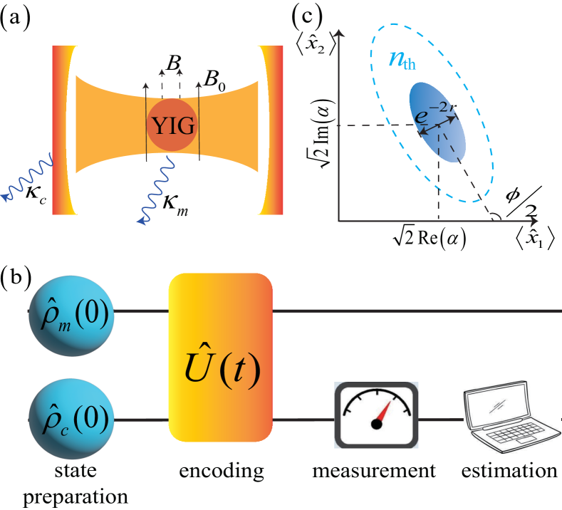
Figure 1: (a) Schematic illustration of the cavity magnonic system: A YIG sphere is placed in a cavity to sense the weak magnetic field $B$, with a bias magnetic field $B_{0}$ applied for magnon excitation. $\kappa_{c}$ and $\kappa_{m}$ represent the damping rates of the cavity and the magnon, respectively. (b) Metrological scheme for estimating the parameter $B$: Quantum dynamics encode the estimated parameter within the covariant matrix, while the measurement is performed on the cavity. (c) Illustration of the Wigner function of a single-mode Gaussian state in terms of displacement, squeezing, phase, and thermalization parameters $(\alpha,r,\phi,n_{\rm th})$.

Role of entanglement in partially accessible metrological schemes– Partially accessible metrological schemes aim to estimate a parameter $B$ from the subsystem $\hat{\rho}_{c}\equiv\mathrm{Tr}_{m}(\hat{\rho}_{cm})$ where $c$ and $m$ represent two distinct subsystems, such as cavity and magnon. Focusing on a pure state for the total system $\hat{\rho}_{cm}$ and assuming a Gaussian state for $\hat{\rho}_{c}$, we express $\hat{\rho}_{c}$ as $\hat{\rho}_{c}\!=\!\hat{D}(\alpha)\hat{S}(\zeta)\hat{\rho}_{\rm th}\hat{S}^{\dagger}(\zeta)\hat{D}^{\dagger}(\alpha)$ FN-Gaussian in terms of the parameters $(\alpha,r,\phi,n_{\rm th})$ Adam95 :

$$\alpha=\frac{1}{\sqrt{2}}(d_{1}^{c}+id_{2}^{c}),\quad r=\frac{1}{2}{\rm arcosh}\left(\frac{\mathrm{Tr}(\gamma^{c})}{2\sqrt{\det(\gamma^{c})}}\right),$$

$$n_{\rm th}=\frac{\sqrt{\det(\gamma^{c})}-1}{2},\quad\tan\phi=\left(\frac{2\gamma_{12}^{c}}{\gamma_{11}^{c}-\gamma_{22}^{c}}\right),$$ (1)

where $d^{c}_{j}\!=\!\langle\hat{x}_{j}\rangle$ is the displacement vector, $\gamma^{c}_{jk}\!=\!\langle\{\hat{x}_{j}\!-\!\langle\hat{x}_{j}\rangle,\hat{x}_{k}\!-\!\langle\hat{x}_{k}\rangle\}\rangle/2$ is the covariance matrix, $\hat{x}_{1}\!=\!(\hat{c}^{\dagger}\!+\!\hat{c})/\sqrt{2}$, $\hat{x}_{2}\!=\!i(\hat{c}^{\dagger}\!-\!\hat{c})/\sqrt{2}$, and $\langle\hat{A}\rangle\!=\!\mathrm{Tr}(\hat{\rho}_{c}\hat{A})$. The parameters $(\alpha,r,\phi,n_{\rm th})$ characterize the displacement, squeezing, phase, and thermalization for subsystem $\hat{\rho}_{c}$, respectively, see Fig. 1(c).

The estimation precision provided by $\hat{\rho}_{c}$ is the Cramér-Rao bound Rao45 ; Cramer46 ; Helstrom67 ; Liu20 , i.e. a lower bound $(\delta B)^{2}\!\geq\!1/F_{Q}(\hat{\rho}_{c})$. In terms of parameters $(\alpha,r,\phi,n_{\rm th})$ FN , we analytically derive the QFI, see Supplemental Material (SM) SM (see also references Paris09 ; Hall15 therein).

$$F_{Q}(\hat{\rho}_{c})\!=\!\frac{4}{2n_{\rm th}+1}\left[\alpha^{\prime}\bar{\alpha}^{\prime}\cosh(2r)\!+\!\text{Re}(\bar{\alpha}^{\prime 2}e^{i\phi})\sinh(2r)\right]$$

$$+\frac{n_{\rm th}^{\prime 2}}{n_{\rm th}(1\!+\!n_{\rm th})}\!+\!\frac{(1+2n_{\rm th})^{2}}{2(1\!+\!2n_{\rm th}\!+\!2n^{2}_{\rm th})}\!\left[\sinh^{2}(2r)\phi^{\prime 2}\!+\!4r^{\prime 2}\right]\!,$$ (2)

where $\bar{\alpha}$ is the complex conjugate of $\alpha$ and the prime denotes derivative with respect to $B$.

If $\hat{\rho}_{c}$ does not arise from critical dynamics, it is justifiable to assume finite values for $(\alpha,r,\phi,n_{\rm th})$ and their respective derivatives. Enhancing measurement precision primarily relies on particle number, i.e., $N_{c}\!\equiv\!|\alpha|^{2}\!+\!n_{\rm th}\!+\!(2n_{\rm th}\!+\!1)\sinh^{2}r$. We first consider the case where particle number is mainly sourced by the displacement, e.g., a coherent state, $N_{c}\!\sim\!|\alpha|^{2}$. Then, Eq. (S21) implies $F_{Q}\!\sim\!\alpha^{\prime}\bar{\alpha}^{\prime}$ leading to the shot noise limit (SNL), i.e., $F_{Q}\!\sim\!N_{c}$. Here it is reasonable to assume that the parameters and their derivatives are of the same order. In the second case, if the thermalized photons dominate, i.e., $N_{c}\!\sim\!n_{\rm th}$ then QFI (S21) does not increase with $N_{c}$ since $F_{Q}\!\sim\!\mathcal{O}(1)$.

Excluding the displacement and thermalized photons as metrological resources, quantum squeezing emerges as a vital resource for surpassing the shot noise limit, also see the study in  Dodonov02 ; Caves81 ; Hollenhorst79 ; Walls83 ; McKenzie02 ; McKenzie04 ; Vahlbruch05 ; Vahlbruch06 . In the third case, assuming that quantum squeezing is dominant then $N_{c}\!\sim\!\sinh^{2}r\!\sim\!e^{2r}$ and $F_{Q}\!\sim\!\sinh^{2}(2r)\!\sim\!e^{4r}$. Explicitly, it achieves HL, $F_{Q}\!\sim\!N_{c}^{2}$. To incorporate the influence of the inevitable thermalization in QFI, we assume the number of thermalized photons scales as $n_{\rm th}\!\sim\!e^{\nu r}$ FN-0 . Equation (S21) reveals that the thermalization does not really affect the scaling of QFI if $n_{\rm th}$ dominates. However, $N_{c}\!\sim\!e^{(2+\nu)r}$ can essentially depend on the thermalization. So QFI exhibits a scaling

$$F_{Q}\!\sim\!N_{c}^{4/(2+\nu)},$$ (3)

which can exceed the SNL if $\nu\!<\!2$.

Bipartite entanglement can be quantified by the entanglement entropy $S(t)\!=\!-\mathrm{Tr}[\hat{\rho}_{c}\log_{2}(\hat{\rho}_{c})]$ Vedral97 . For Gaussian states, it reduces to Agarwal71

$$S(t)=\log_{2}(n_{\rm th}+1)+n_{\rm th}\log_{2}\left(\frac{n_{\rm th}+1}{n_{\rm th}}\right),$$ (4)

showing that entanglement increases with the number of thermalized photons $n_{\rm th}$ grows. Combining Eqs. (3) and (4), we deduce that the existence of bipartite entanglement decreases the final measurement precision. Nevertheless, in order to achieve scaling law (3), the parameters are required to be encoded effectively in the covariance matrix of the subsystem $\hat{\rho}_{c}$. The emergent entanglement guarantees such an encoding from a product state, thus highlighting the significance of bipartite entanglement in the dynamical encoding process. This finding establishes fundamental laws governing the role of bipartite entanglement in partially accessible Gaussian metrology.

Quantum Measurements.– Now we discuss how to experimentally realize the measurement precision given by the Cramér-Rao bound. Based on the Gaussian measurements, the CFI is obtained as follows SM (see also reference Monras06 therein).

$$F_{C}(\hat{\rho}_{c}) =\frac{[n^{\prime}_{\rm th}-(2n_{\rm th}+1)r^{\prime}]^{2}}{2(n_{\rm th}+1)^{2}}+\frac{[n^{\prime}_{\rm th}+(2n_{\rm th}+1)r^{\prime}]^{2}}{2(n_{\rm th}+1)^{2}}$$

$$+\frac{(2n_{\rm th}+1)^{2}[\phi^{\prime}\sinh(2r)]^{2}}{4(n_{\rm th}+1)^{2}},$$ (5)

where we only considered quantum states with zero displacement. Equation (S30) reveals that the scaling of CFI matches that of QFI, demonstrating that Gaussian measurements are optimal. Experimentally, after acquiring probabilities through Gaussian measurements, we can utilize the maximum likelihood estimator to estimate the unknown parameter Rossi18 . Implementing Gaussian measurements involves two steps: applying a Gaussian unitary operation to the input system, which includes additional ancillary (vacuum) modes, and performing homodyne measurements on all output modes Weedbrook12 ; Giedke02 ; Eisert03 . Next, we will apply these general results to a cavity magnonic system, exploring distinct roles of entanglement in dynamic encoding and measurement processes.

Model.– We consider a system consisting of a Yttrium iron garnet (YIG) sphere placed inside a microwave cavity and subjected to a static magnetic field, $B_{0}$ Tabuchi14 ; Zhang14 see Fig. 1(a). The microwave field induces magnon excitations in the ferromagnetic YIG sphere. Additionally, we introduce a weak field $B$ for estimation. Using the Holstein-Primakoff approximation Holstein40 , the corresponding Hamiltonian is given by Zhang14 ; FN-2

$$\hat{H}=\omega_{c}\hat{c}^{\dagger}\hat{c}+\omega_{m}\hat{b}^{\dagger}\hat{b}+g(\hat{c}+\hat{c}^{\dagger})(\hat{b}+\hat{b}^{\dagger}),$$ (6)

where $\hat{c}^{\dagger}$ $(\hat{b}^{\dagger})$ and $\hat{c}$ $(\hat{b})$ are creation and annihilation operators for the cavity photon (magnon) at frequency $\omega_{c}$ [$\omega_{m}\!=\!\mu(B_{0}\!+\!B)]$, respectively. The gyromagnetic ratio $\mu$ is set to 1 and $g$ is the coupling strength. The Hamiltonian (6) applies to the ferromagnetic YIG sphere only when $g\!<\!g_{c}\!\equiv\!\sqrt{\omega_{c}\omega_{m}}/2$ Emary03 . Beyond the critical point $g_{c}$, the system remains in the super-radiant phase.

The metrological scheme is shown in Fig. 1(b), where the initial magnon-cavity state is prepared in a product state $\hat{\rho}_{cm}(0)\!=\!\hat{\rho}_{c}(0)\otimes\hat{\rho}_{m}(0)$. Over time, the information of the weak field $B$ becomes encoded in the state $\hat{\rho}_{cm}(t)\!=\!\exp(-iHt)\hat{\rho}_{cm}(0)\exp(iHt)$. At time $t_{*}$, we perform Gaussian measurements on the cavity state $\hat{\rho}_{c}(t_{*})\!=\!\mathrm{Tr}_{m}[\hat{\rho}_{cm}(t_{*})]$ and estimate the value of $B$ from the measurement results.

Far away from critical dynamics.– When $|\omega_{c}-\omega_{m}|\ll 1$ and $g\ll g_{c}$, we can employ the rotating wave approximation (6) to rewrite the Hamiltonian as

$$\hat{H}=\omega_{c}\hat{c}^{\dagger}\hat{c}+\omega_{m}\hat{b}^{\dagger}\hat{b}+g\left(\hat{c}^{\dagger}\hat{b}+\hat{c}\hat{b}^{\dagger}\right).$$ (7)

Its dissipative dynamics is described by the quantum Langevin equation

$$\partial_{t}\hat{c}(t)=-i\omega_{c}\hat{c}(t)-ig\hat{b}(t)-\frac{\kappa_{c}}{2}\hat{c}(t)+\sqrt{\kappa_{c}}\hat{c}_{\rm in}(t),$$

$$\partial_{t}\hat{b}(t)=-i\omega_{m}\hat{b}(t)-ig\hat{c}(t)-\frac{\kappa_{m}}{2}\hat{b}(t)+\sqrt{\kappa_{m}}\hat{b}_{\rm in}(t),$$ (8)

where $\kappa_{c}$ and $\kappa_{m}$ denote the damping rates of the cavity mode and the magnon mode, respectively. The input noises are described by the annihilation operators $\hat{c}_{\rm in}$ and $\hat{b}_{\rm in}$, satisfying $\langle\hat{c}^{\dagger}_{\rm in}(t_{1})\hat{c}_{\rm in}(t_{2})\rangle\!=\!n_{c}\delta(t_{1}\!-\!t_{2})$ and $\langle\hat{b}^{\dagger}_{\rm in}(t_{1})\hat{b}_{\rm in}(t_{2})\rangle\!=\!n_{m}\delta(t_{1}\!-\!t_{2})$. Here the values of $n_{c}$ and $n_{m}$ are subject to external environment thermal noise. For simplicity, we assume $\kappa_{m}\!=\!\kappa_{c}$ and $n_{m}\!=\!n_{c}$.

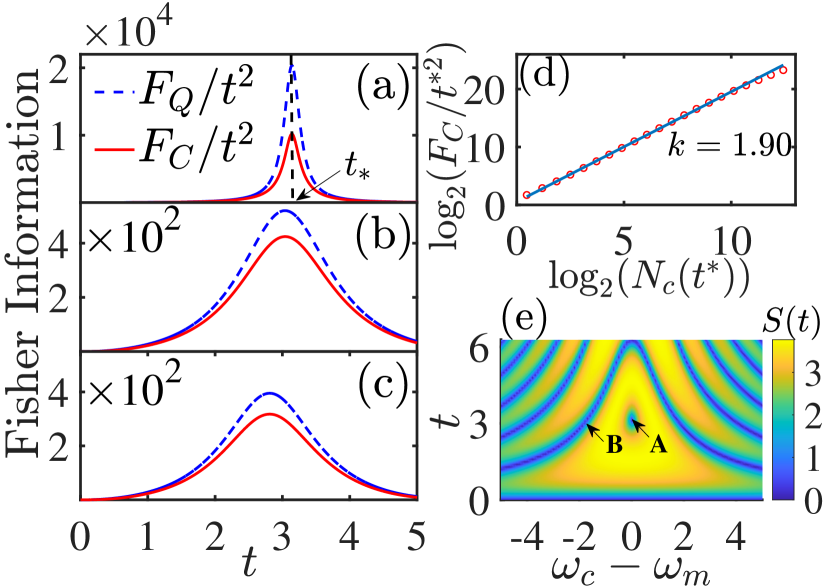
Figure 2: Time evolution of the time-rescaled QFI $F_{Q}/t^{2}$ (blue dotted line) and CFI $F_{C}/t^{2}$ (red line) in (a) resonance case $\omega_{c}\!=\!\omega_{m}\!=\!2,\kappa_{c}\!=\!n_{c}\!=\!0$, (b) dissipated case $\omega_{c}\!=\!\omega_{m}=2,\kappa_{c}\!=\!0.001,n_{c}\!=\!30$, and (c) off-resonance case $\omega_{c}\!=\!2,\omega_{m}\!=\!2.5$, $\kappa_{c}\!=\!n_{c}\!=\!0$. (d) Scaling law of the CFI ($F_{C}\!\sim\!N_{c}^{k}$ with $k\!=\!{1.90}$) for the parameter setting used in the experiment Bourhill16 : $\omega_{c}\!=\!\omega_{m}\!=\!15.506\times 2\pi$ GHZ, $g\!=\!7.11\!\times\!\pi$ GHZ, and $\kappa_{c}\!=\!\kappa_{m}\!=\!1.029\!\times\!\pi$ MHZ. $t_{*}$ denotes the time of the CFI peak and $N_{c}(t_{*})$ is the number of photons at that moment. (e) Time evolution of entanglement $S(t)$ versus the detuning $\omega_{c}\!-\!\omega_{m}$.

The initial state is chosen with the cavity in the vacuum state $|0\rangle$ and the magnon in a squeezed vacuum state $\hat{\rho}_{m}(0)\!=\!\hat{S}(r_{0})|0\rangle\langle 0|\hat{S}^{\dagger}(r_{0})$, which can be generated via parametric pumping Li19 ; Demokritov06 ; Zhang21 . The quantum Langevin equation (III.1) is analytically solved and the evolution of $\hat{\rho}_{c}(t)$ can be divided into two processes SM :

$$\hat{\rho}_{c}(0)\xrightarrow[\rm P1]{\rm no\,noise}\hat{\rho}_{\rm in}(t)\xrightarrow[\rm P2]{\rm noise}\hat{\rho}_{c}(t),$$ (9)

where $\hat{\rho}_{\rm in}(t)$ denotes the cavity state in noiseless case. During the evolution the displacement of $\hat{\rho}_{c}(t)$ is always zero. Focusing on the corresponding covariance matrices, we find SM

$${\rm P1}:\ \gamma_{\rm in}^{c}(t)=\xi(t)\gamma^{c}_{\rm sq}+[1-\xi(t)]\mathds{1}_{2},$$

$${\rm P2}:\ \gamma^{c}(t)=\eta(t)\gamma^{c}_{\rm in}(t)+[1-\eta(t)](2n_{c}+1)\mathds{1}_{2},$$ (10)

where $\gamma^{c}_{\rm sq}$ is the covariance matrix of the squeezed state $\hat{S}(-r_{0}e^{-i(\omega_{c}+\omega_{m})t})|0\rangle$, $r_{0}$ is the squeeing parameter of the initial magnon state, $\gamma_{\rm in}^{c}(t)$ and $\gamma^{c}(t)$ are the covariance matrices of $\hat{\rho}_{\rm in}(t)$ and $\hat{\rho}_{c}(t)$, respectively. Here $\eta(t)\!=\!\exp(-\kappa_{c}t)$, $\xi(t)\!=\!4g^{2}\sin^{2}(\Delta t/2)/\Delta^{2}$, and $\Delta\!=\!\sqrt{4g^{2}+(\omega_{c}-\omega_{m})^{2}}$.

In the dissipative process P2, equation (Quantum-Enhanced Metrology in Cavity Magnomechanics) implies that $\gamma^{c}(t)$ tends toward a thermal state $(2n_{c}+1)\mathds{1}_{2}$ since $\lim_{t\to\infty}\eta(t)=0$. This process indicates the gradual dissipation of information into the external environment, resulting in measurement precision described by the QFI (CFI) being smaller than the non-dissipative case, see Fig. 2(a,b).

Unlike process P2, process P1 describes the flow of the magnetic field information between the cavity and the magnon. At $t\!=\!0$, the cavity is only a vacuum state without any quantum resources and information. Then the appearance of the dynamics-induced bipartite entanglement essentially lead to the transmission of information from the squeezed magnon state into the cavity, see Fig. 2(e). From Eq. (Quantum-Enhanced Metrology in Cavity Magnomechanics), we observe that the cavity state finally becomes a squeezed state $\hat{S}(-r_{0}e^{-i(\omega_{c}+\omega_{m})t})|0\rangle$ Footnote at a time $t_{*}\!=\!\pi/(2g)$ satisfying $\xi(t_{*})\!=\!1$. This condition is satisfied only for the resonant case. It is crucial to emphasize that at this special time $t_{*}$, the whole system $\hat{\rho}_{cm}(t_{*})$ is in a non-entangled state, yet both the information $\omega_{m}$ and the initial squeezing resource $r_{0}$ have been completely transferred to the cavity part without thermalization. Thus, the HL-precision, ($F_{C}\!\sim\!N_{c}^{2}$), can be achieved in the absence of noise by Eq. (3). Using experimental parameters Bourhill16 , we show that the precision still remains near HL, specifically $F_{C}\!\sim\!N_{c}^{1.90}$ as shown in Fig. 2(d). Here, the Gilbert damping of magnons $\kappa_{m}/\omega_{m}$ is on the order of $10^{-3}$ Bourhill16 ; Wu21 .

If the estimated weak magnetic field $\vec{B}$ deviates from the bias field $\vec{B}_{0}$ along the $z$-axis, the Hamiltonian (S31) acquires an additional term $\!-\!(B_{x}\!-\!iB_{y})\hat{b}/2\!-\!(B_{x}\!+\!iB_{y})\hat{b}^{\dagger}/2$. In SM SM , we show that these nonparallel components contribute to the displacement of the evolved Gaussian state and their impact on QFI is limited to the SNL. Significantly, the nonvanishing parallel component effectively encodes information into the covariance matrix, leading to QFI following HL. Consequently, in our subsequent discussion, we can safely disregard the nonparallel components SM . Based on soykal:PRB2010 , crystalline anisotropy becomes notable in nanomagnets around 2nm radius. However, the YIG sphere considered here has a 360nm diameter Zhang14 . Thus, the effect of crystalline anisotropy can be disregarded.

The significance of dynamic entanglement in encoding information process becomes clearer through a contrasting example where the inputs are magnon and cavity squeezed coherent states with identical squeezing parameters. In this setup, no bipartite entanglement will be generated, indicating that information $B$ cannot be efficiently encoded into the phase parameter and is solely in the displacement parameter. Based on the analysis below Eq. (4), the precision cannot surpass the SNL, even in the presence of squeezing.

Returning to the initial scenario, however, entanglement during the measurement process will introduce thermalization, see Eq. (4). Consequently, the initial squeezing resource $r_{0}$ cannot be fully transferred to the cavity, disrupting the HL precision. Figure 2 (e) shows the entanglement evolution concerning the detuning parameter $\omega_{c}-\omega_{m}$. Vanishing entanglement in the curve B (blue) indicates the quantum state periodically returns to the initial state. A nontrivial situation occurs in the resonant region A where entanglement vanishes after encoding the information into the cavity’s covariance matrix, ensuring the realization of HL precision. Far away from region A, increasing detuning leads to strong entanglement between the cavity and the magnon, thus failing to suppress SNL, see Fig. 2 (a,c).

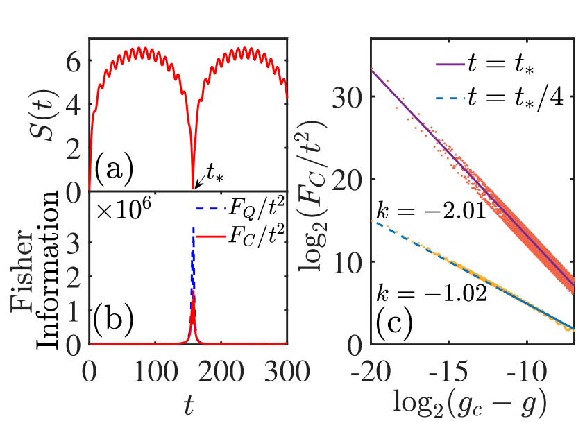
Figure 3: Time evolution of (a) entanglement $S(t)$, (b) time-rescaled QFI $F_{Q}/t^{2}$, and CFI $F_{C}/t^{2}$ for critical dynamics. (c) Scaling of CFI: $F_{C}\sim(g_{c}-g)^{k}$ with $k=-2.01$ for $t=t_{*}$ and $k=-1.02$ for $t=t_{*}/4$. Lines in (c) are the results of fitting the theoretical data. Other parameters are $\omega_{c}\!=\!\omega_{m}\!=\!2$, $g\!=\!0.9999g_{c}$, and $t_{*}\!=\!\pi/\epsilon_{-}$.

Critical dynamics.– In the strong coupling regime, Hamiltonian (6) is directly diagonalizable as $\hat{H}\!=\!\epsilon_{-}\hat{c}^{\dagger}_{1}\hat{c}_{1}\!+\!\epsilon_{+}\hat{c}^{\dagger}_{2}\hat{c}_{2}$ using the Bogoliubov transformation Emary03 . The normal-to-superradiant phase transition occurs at the critical point $g_{c}\!=\!\sqrt{\omega_{c}\omega_{m}}/2$. Near this point ($g\!\to\!g_{c}$), the excitation energy of the photon branch scales as $\epsilon_{-}\!\sim\!(g_{c}-g)^{1/2}$ and its derivative plays a crucial role in achieving criticality-enhanced metrology. Thus, in contrast to the weak coupling case, no specific resource state is required and we can choose the vacuum states as inputs.

Using Eqs. (S12, S21, S30), we derived the analytic expression of the covariance matrix $\gamma^{c}(t)$ in SM . There is a special time $t_{*}=n\pi/\epsilon_{-}$ $(n\in\mathbb{Z}_{>0})$ at which the covariance matrix $\gamma^{c}(t_{*})$ is finite otherwise it diverges. It then follows from Eq. (S12) that the divergence of $\gamma^{c}$ at $t\neq t_{*}$ implies the divergence of the number of thermalized particles $n_{\rm th}$, e.g., $n_{\rm th}(t_{*}/4)\!\sim\!(g_{c}-g)^{-1/2}$ SM . Therefore, by the relation (4) we find that the magnon-photon entanglement $S(t)$ becomes large at $t\neq t_{*}$ but almost disappears suddenly at $t=t_{*}$, see Fig. 3(a).

Figure 3(b) shows that the measurement precision has a maximum at the time $t_{*}$, meanwhile the entanglement almost disappears at $t=t_{*}$. In this sense, the vanishing entanglement in the measurement process enhances the measurement precision. More rigorously, we obtain critical scalings of the relevant parameters SM-2 and QFI:

$$F_{Q}(t_{*})\sim F_{C}(t_{*})\sim(g_{c}-g)^{-2}t_{*}^{2},$$

$$F_{Q}(t_{*}/4)\sim F_{C}(t_{*}/4)\sim(g_{c}-g)^{-1}t_{*}^{2},$$ (11)

which are further confirmed by numerical results shown in Fig. 3(c).

It is worth noting that, compared with the $t_{*}$ case, the divergent squeezing $[\cosh(2r)\!\sim\!(g_{c}-g)^{-1/2}]$ in $t_{*}/4$ case causes no further enhancement in measurement precision. This is mainly because such a divergence in the covariance matrix also leads to a strong entanglement that makes the cavity state more insensitive to the estimated parameter, see the scalings of $r^{\prime}$ and $\phi^{\prime}$ in SM-2 .

Conclusion.– The usable bipartite entanglement in accessible metrological schemes has been established by linking Fisher information to entanglement. We have elaborated on the significance of entanglement in the efficient encoding process for high-precision quantum estimation, particularly starting from the initial product state. While unveiling the adverse impact of entanglement on the final measurement process. These findings enable us to design quantum-enhanced estimations within an experimentally feasible cavity magnonics system. In particular, we have proposed an approach to realizing the precision of the HL in the weak coupling regime. Regarding strong coupling, we have demonstrated that the criticality-enhanced metrology should attribute to the criticality-induced parameter sensitivity rather than criticality-induced squeezing. Our protocols show a potential application of quantum metrology through current experimental cavity magnonic systems Wolski20 ; Silaev23 ; Rao23 ; Golovchanskiy21-1 ; Kockum19 ; Boventer18 ; Golovchanskiy21 ; Kostylev16 ; You23 , enabling quantum-enhanced metrology with or without a particular squeezed initial state.

Supplemental Material for “Quantum Metrology in Cavity Magnomechanics”

Qing-Kun Wan, Hai-Long Shi, and Xi-Wen Guan

I I. Hamiltonian of the Cavity magnomechanical system

In pursuit of self-consistency, we will first derive the Hamiltonian describing the cavity magnomechanical system by employing the standard Holstein-Primakoff transformation method Holstein40 , see also references Yuan22 and Yuan20 . The Hamiltonian of the cavity magnomechanical system takes the form $\hat{H}=\hat{H}_{\text{FM}}+\hat{H}_{\text{ph}}+\hat{H}_{\text{int}}$:

$$\hat{H}_{\text{FM}}=-J\sum_{\left\langle i,j\right\rangle}\vec{S_{i}}\cdot\vec{S}_{j}-\mu\sum_{i}(B_{0}\hat{S}_{i}^{z}+\vec{B}\cdot\vec{S}_{i}),$$

$$\hat{H}_{\rm ph}=\frac{1}{2}\int(\epsilon_{0}\vec{E}_{\rm ph}^{2}+\mu_{0}\vec{H}_{\rm ph}^{2})d\vec{r},\quad\hat{H}_{\text{int}}=-\sum_{i}\vec{S}_{i}\cdot\vec{H}_{\rm ph},$$ (S1)

where $\hat{H}_{\text{FM}}$, $\hat{H}_{\text{ph}}$, and $\hat{H}_{\text{int}}$ are the Hamiltonians for the ferromagnet material, the optical cavity, and their interaction, respectively. Here, $J>0$ is the exchange constant; $\left\langle i,j\right\rangle$ denotes the nearest neighbor spins; $\mu$ is gyromagnetic ratio; $B_{0}$ is a strong polarized magnetic field; $\vec{B}=(B_{x},B_{y},B_{z})$ is the estimated weak magnetic field; $\vec{E}_{p}$ and $\vec{H}_{p}$ are electric field and magnetic field of the electromagnetic wave; $\epsilon_{0}$ and $\mu_{0}$ are vacuum permittivity and susceptibility.

Using the Holstein-Primakoff transformation:

$$\hat{S}_{i}^{z}=S-\hat{b}^{\dagger}_{i}\hat{b}_{i},\quad\hat{S}_{i}^{x}=\sqrt{\frac{S}{2}}(\hat{b}_{i}+\hat{b}_{i}^{\dagger}),\quad\hat{S}_{i}^{y}=-i\sqrt{\frac{S}{2}}(\hat{b}_{i}-\hat{b}_{i}^{\dagger}),$$ (S2)

and the Fourier transformation:

$$\hat{b}_{i}=1/\sqrt{N}\sum_{k}\exp(i\vec{k}\cdot\vec{r}_{i})\hat{b}_{k},$$ (S3)

we can reformulate $\hat{H}_{\rm FM}$ in terms of the bosonic operators $\hat{b}$ and $\hat{b}^{\dagger}$ as follows

$$\hat{H}_{\text{FM}}=4JS\sum_{k}(1-\cos(kd))\hat{b}_{k}^{\dagger}\hat{b}_{k}+\mu(B_{0}+B_{z})\hat{b}_{k}^{\dagger}\hat{b}_{k}-\mu\sqrt{\frac{S}{2}}(B_{x}-iB_{y})\hat{b}_{k=0}-\mu\sqrt{\frac{S}{2}}(B_{x}+iB_{y})\hat{b}^{\dagger}_{k=0},$$ (S4)

where $d$ is lattice constant. To quantize electromagnetic field, we introduce the vector potential operator:

$$A(\vec{r},t)=\sum_{k}\sqrt{\frac{\hbar}{2\omega_{k}\epsilon_{0}}}(\hat{a}_{k}\vec{u}_{k}(r)e^{-i\omega_{k}t}-\text{h.c.}).$$ (S5)

Subsequently, utilizing the formulas $\vec{E}_{\rm ph}=-\frac{\partial}{\partial t}A(\vec{r},t)$ and $\vec{H}_{\rm ph}=\frac{1}{\mu_{0}}\nabla\times A$, we obtain

$$\hat{H}_{\text{ph}}=\sum_{k}\frac{\omega_{k}\hbar}{2}(\hat{c}_{k}^{\dagger}\hat{c}_{k}+\hat{c}_{k}\hat{c}_{k}^{\dagger}).$$ (S6)

By substituting Eqs. (S2), (S3) and (S5) into the Hamiltonian of the interaction, we have

$$\hat{H}_{\text{int}}=g\sum_{k}(\hat{b}_{k}\hat{c}_{k}^{\dagger}+\hat{b}_{k}^{\dagger}\hat{c}_{k}+\hat{b}_{k}\hat{c}_{-k}+\hat{b}_{k}^{\dagger}\hat{c}_{-k}^{\dagger}),$$ (S7)

where $g$ is the coupling constant. As the photon can only couple with the magnon around $k=0$, the total Hamiltonian simplifies to

$$\hat{H}=\omega_{c}\hat{c}^{\dagger}\hat{c}+\omega_{m}\hat{b}^{\dagger}\hat{b}+g(\hat{c}+\hat{c}^{\dagger})(\hat{b}+\hat{b}^{\dagger})-\mu\frac{B_{x}-iB_{y}}{2}\hat{b}-\mu\frac{B_{x}+iB_{y}}{2}\hat{b}^{\dagger},$$ (S8)

where $\omega_{m}=\mu(B_{0}+B_{z})$ and $B_{x},B_{y}$ are the magnetic anisotropy. We address the case of magnetic anisotropy only in Section III; otherwise, we assume $B_{x}=B_{y}=0$.

II II. Fisher Information for general single-mode Gaussian States

During the dynamical evolution, the cavity state $\hat{\rho}_{c}$ keeps in the Gaussian form and thus can be fully characterized by the displacement vector $\vec{d}^{c}=(\langle\hat{X}_{c}\rangle,\langle\hat{P}_{c}\rangle)$ and the covariance matrix

$$\gamma^{c}=\begin{pmatrix}2\langle\hat{X}_{c}^{2}\rangle-2\langle\hat{X}_{c}\rangle^{2}&\langle\{\hat{X}_{c},\hat{P}_{c}\}\rangle-2\langle\hat{X}_{c}\rangle\langle\hat{P}_{c}\rangle\\ \langle\{\hat{X}_{c},\hat{P}_{c}\}\rangle-2\langle\hat{X}_{c}\rangle\langle\hat{P}_{c}\rangle&2\langle\hat{P}_{c}^{2}\rangle-2\langle\hat{P}_{c}\rangle^{2}\end{pmatrix},$$ (S9)

where $\{\hat{A},\hat{B}\}:=\hat{A}\hat{B}+\hat{B}\hat{A}$, $\langle\hat{A}\rangle:=\mathrm{Tr}(\hat{\rho}_{c}\hat{A})$, $\hat{X}_{c}=(\hat{c}^{\dagger}+\hat{c})/\sqrt{2}$, and $\hat{P}_{c}=i(\hat{c}^{\dagger}-\hat{c})/\sqrt{2}$. Furthermore, arbitrary single-mode Gaussian state can be rewritten as a displaced squeezed thermal state Adam95 , i.e.,

$$\hat{\rho}_{c}=\hat{D}(\alpha)\hat{S}(\zeta)\hat{\rho}_{\rm th}\hat{S}^{\dagger}(\zeta)\hat{D}^{\dagger}(\alpha),$$ (S10)

where $\hat{D}(\alpha)=\exp(\alpha\hat{c}^{\dagger}-\bar{\alpha}\hat{c})$ is the displacement operator with $\alpha\in\mathbb{C}$, $\hat{S}(\zeta)=\exp(-\zeta\hat{c}^{\dagger 2}/2+\bar{\zeta}\hat{c}^{2}/2)$ is the squeezing operator with $\zeta=r\exp(i\phi)$ ($r\geq 0$), and $\hat{\rho}_{\rm th}=\sum_{n}P_{n}|n\rangle\langle n|$ is a thermal state with $P_{n}=n_{\rm th}^{n}/(1+n_{\rm th})^{1+n}$ and $|n\rangle$ being the Fock states. Substituting Eq. (S10) into Eq. (S9) we obtain

$$d_{1}^{c}=\sqrt{2}\text{Re}(\alpha),\quad d_{2}^{c}=\sqrt{2}\text{Im}(\alpha),$$

$$\gamma^{c}_{11}=(2n_{\rm th}+1)[\cosh(2r)-\sinh(2r)\cos(\phi)],$$

$$\gamma^{c}_{22}=(2n_{\rm th}+1)[\cosh(2r)+\sinh(2r)\cos(\phi)],$$

$$\gamma^{c}_{12}=\gamma^{c}_{21}=-(2n_{\rm th}+1)\sinh(2r)\sin(\phi),$$ (S11)

and then we can determine $(\alpha,r,\phi,n_{\rm th})$ in terms of the displacement vector $\vec{d}^{c}$ and the elements of the covariance matrix $\gamma^{c}$ as follows

$$\alpha=\frac{1}{\sqrt{2}}(d_{1}^{c}+id_{2}^{c}),\quad n_{\rm th}=\frac{\sqrt{\det(\gamma^{c})}-1}{2},\quad r=\frac{1}{2}{\rm arcosh}\left(\frac{\mathrm{Tr}(\gamma^{c})}{2\sqrt{\det(\gamma^{c})}}\right)\geq 0,\ {\rm and}\ \tan\phi=\left(\frac{2\gamma_{12}^{c}}{\gamma_{11}^{c}-\gamma_{22}^{c}}\right).$$ (S12)

Next, we will derive quantum Fisher information (QFI) and classical Fisher information (CFI) for single Gaussian states (S10) and express them in terms of parameters $(\alpha,r,\phi,n_{\rm th})$. The QFI is defined as

$$F_{Q}:=\mathrm{Tr}(\hat{\rho}_{c}\hat{L}^{2}),$$ (S13)

where $\hat{L}$ is symmetric logarithmic derivative (SLD) operator. By rewriting the cavity state as the standard form (S10) $\hat{\rho}_{c}=\sum_{n}P_{n}|\Psi_{n}\rangle\langle\Psi_{n}|$ with $|\Psi_{n}\rangle=\hat{D}(\alpha)\hat{S}(\zeta)|n\rangle$ and $P_{n}=n_{\rm th}^{n}/(1+n_{\rm th})^{1+n}$, the SLD operator is given by Paris09

$$\hat{L} = \sum_{n}\frac{\partial_{B}P_{n}}{P_{n}}|\Psi_{n}\rangle\langle\Psi_{n}|+2\sum_{n,m}\frac{P_{n}-P_{m}}{P_{n}+P_{m}}\langle\Psi_{m}|\partial_{B}\Psi_{n}\rangle|\Psi_{m}\rangle\langle\Psi_{n}|,$$ (S14)

where the parameter $B$ is to be estimated and $\partial_{B}:=\partial/\partial_{B}$. By using the following formula Hall15 :

$$\partial_{B}\left(e^{\hat{O}}\right) = \int_{0}^{1}e^{s\hat{O}}\left(\partial_{B}\hat{O}\right)e^{(1-s)\hat{O}}ds,$$ (S15)

we obtain

$$\partial_{B}\hat{D}(\alpha)=\left[\alpha^{\prime}\hat{c}^{\dagger}-\bar{\alpha}^{\prime}\hat{c}+\frac{1}{2}\alpha\bar{\alpha}^{\prime}-\frac{1}{2}\bar{\alpha}\alpha^{\prime}\right]\hat{D}(\alpha),$$

$$\partial_{B}\hat{S}(\xi)=\left[-\frac{\xi^{\prime}}{2}\left(\left[\frac{\sinh(2r)}{4r}+\frac{1}{2}\right]\hat{c}^{\dagger 2}+e^{-2i\phi}\left[\frac{\sinh(2r)}{4r}-\frac{1}{2}\right]\hat{c}^{2}+e^{-i\phi}\left[\frac{\cosh(2r)}{4r}-\frac{1}{4r}\right](\hat{c}^{\dagger}\hat{c}+\hat{c}\hat{c}^{\dagger})\right)-h.c.\right]\hat{S}(\xi),$$

where ^′ denotes $\partial_{B}$ and $\xi=r\exp(i\phi)$. Using Eq. (II) we obtain

$$\langle\Psi_{m}|\partial_{B}\Psi_{n}\rangle = \langle m|\hat{S}^{\dagger}(\xi)\hat{D}^{\dagger}(\alpha)([\partial_{B}\hat{D}(\alpha)]\hat{S}(\xi)+\hat{D}(\alpha)[\partial_{B}\hat{S}(\xi)])|n\rangle$$ (S17)

$$= A_{1}\delta_{n,m-1}-\bar{A}_{1}\delta_{n,m+1}+A_{2}\delta_{n,m-2}-\bar{A}_{2}\delta_{n,m+2},$$

where

$$A_{1} = \alpha^{\prime}\cosh(r)+\bar{\alpha}^{\prime}\exp(i\phi)\sinh(r),\quad A_{2}=-\frac{i\phi^{\prime}}{4}\exp(i\phi)\sinh(2r)-\frac{r^{\prime}}{2}\exp(i\phi).$$ (S18)

Substituting Eqs. (S17), (S18), and $P_{n}=n_{\rm th}^{n}/(1+n_{\rm th})^{1+n}$ into Eq. (S14), we obtain the following expression of the SLD operator

$$\hat{L} = \hat{D}(\alpha)\hat{S}(\xi)\left(\hat{L}_{0}+\hat{L}_{1}+\hat{L}_{2}\right)\hat{S}^{\dagger}(\xi)\hat{D}^{\dagger}(\alpha),$$ (S19)

where

$$\hat{L}_{0}=\frac{\hat{c}^{\dagger}\hat{c}-n_{\rm th}}{n_{\rm th}(1+n_{\rm th})}n_{\rm th}^{\prime},$$

$$\hat{L}_{1}=\frac{2}{1+2n_{\rm th}}\left([\alpha^{\prime}\cosh(r)+\bar{\alpha}^{\prime}e^{i\phi}\sinh(r)]\hat{c}^{\dagger}+[\bar{\alpha}^{\prime}\cosh(r)+\alpha^{\prime}e^{-i\phi}\sinh(r)]\hat{c}\right),$$

$$\hat{L}_{2}=\frac{2(1+2n_{\rm th})}{1+2n_{\rm th}+2n_{\rm th}^{2}}\left(\left[-\frac{i\phi^{\prime}}{4}e^{i\phi}\sinh(2r)-\frac{r^{\prime}}{2}e^{i\phi}\right]\hat{c}^{\dagger 2}+\left[\frac{i\phi^{\prime}}{4}e^{-i\phi}\sinh(2r)-\frac{r^{\prime}}{2}e^{-i\phi}\right]\hat{c}^{2}\right).$$ (S20)

Finally, by substituting Eq. (S19) into the definition of the QFI (S13) we obtain

$$F_{Q} = \frac{n_{\rm th}^{\prime 2}}{n_{\rm th}(1+n_{\rm th})}+\frac{4}{2n_{\rm th}+1}\left[\alpha^{\prime}\bar{\alpha}^{\prime}\cosh(2r)+\text{Re}(\bar{\alpha}^{\prime 2}e^{i\phi})\sinh(2r)\right]$$ (S21)

$$+\frac{(1+2n_{\rm th})^{2}}{2(1+2n_{\rm th}+2n^{2}_{\rm th})}\left[\sinh^{2}(2r)\phi^{\prime 2}+4r^{\prime 2}\right],$$

where the first term only depends on the thermalization parameter $n_{\rm th}$, the displacement parameter $\alpha$ only affects the second term, and the last term is closely related with the squeezing parameter $\xi=re^{i\phi}$.

For the metrology scheme based on the Gaussian measurements, we use CFI to evaluate its performance, which is defined as

$$F_{C}:=\int d^{2}\chi\frac{[\partial_{B}p(\chi|B)]^{2}}{p(\chi|B)},$$ (S22)

where $p(\chi|B)=\mathrm{Tr}[\hat{\rho}_{c}\hat{\Pi}(\chi)]$ is the probability of obtaining measurement outcome $\chi=(q,p)$ by performing the Gaussian measurements on the cavity state $\hat{\rho}_{c}$. A general Gaussian measurement is given by

$$\hat{\Pi}(\chi)=\frac{1}{2\pi}\hat{D}(\chi)\hat{\Pi}_{0}\hat{D}^{\dagger}(\chi),$$ (S23)

where $\hat{\Pi}_{0}$ is a density matrix of a single-mode Gaussian state and $\hat{D}(\chi)=\exp[i(p\hat{X}_{c}-q\hat{P}_{c})]$ is the displacement operator. Without losing generality, here we set $\vec{d}^{c}=0$. The the CFI (S22) can be rewritten as Monras06

$$F_{C}=\frac{1}{2}\mathrm{Tr}[M(M^{-1})^{\prime}M(M^{-1})^{\prime}],$$ (S24)

where the prime denotes the derivative of $M^{-1}=(\gamma^{c}+\gamma^{0})$ w.r.t the weak magnetic field $B$ and $\gamma^{0}$ denotes the covariance matrix of the Gaussian state $\hat{\Pi}_{0}$.

It follows from Eq. (II) that the covariance matrix of the cavity state can be rewritten as

$$\gamma^{c} = (2n_{\rm th}+1)R^{T}(\phi)T(r)R(\phi),$$ (S25)

where

$$R(\phi)=\begin{pmatrix}\cos(\phi/2)&\sin(\phi/2)\\ -\sin(\phi/2)&\cos(\phi/2)\end{pmatrix},\quad T(r)=\begin{pmatrix}e^{-2r}&0\\ 0&e^{2r}\end{pmatrix}.$$ (S26)

Notice that different choices of $\gamma^{0}$ determine different Gaussian measurements. We restrict $\hat{\Pi}_{0}$ to a squeezed vacuum state and parameterize its covariant matrix $\gamma^{0}$ in terms of $\psi$ and $s$, i.e., $\gamma^{0}=R^{T}(\psi)T(s)R(\psi)$. Substituting these conditions into Eq. (S24) we obtain

$$F_{C}=\frac{1}{2}\text{Tr}\left(M(M^{-1})^{\prime}M(M^{-1})^{\prime}\right)=\frac{1}{2}\text{Tr}\left(\Gamma^{-1}\Sigma\Gamma^{-1}\Sigma\right),$$ (S27)

where

$$\Gamma = R(\phi)(\gamma^{0}+\gamma^{c})R^{T}(\phi)$$

$$= R^{T}(\psi-\phi)T(s)R(\psi-\phi)+(2n_{\rm th}+1)T(r)$$

$$= [\sinh(2s)\sin(\phi-\psi)]\sigma_{x}-[(2n_{\rm th}+1)\sinh(2r)+\cos(\phi-\psi)\sinh(2s)]\sigma_{z}$$

$$+[(2n_{\rm th}+1)\cosh(2r)+\cosh(2s)]\mathds{1}_{2},$$

$$\Sigma = R(\phi)(\gamma^{0}+\gamma^{c})^{\prime}R^{T}(\phi)$$ (S28)

$$= 2n_{\rm th}^{\prime}T(r)-2(2n_{\rm th}+1)r^{\prime}\sigma_{z}T(r)+(2n_{\rm th}+1)\frac{\phi^{\prime}}{2}[R^{T}(\pi)T(r)+T(r)R(\pi)]$$

$$= -(2n_{th}+1)\phi^{\prime}\sinh(2r)\sigma_{x}-2[n^{\prime}_{\rm th}\sinh(2r)+(2n_{\rm th}+1)r^{\prime}\cosh(2r)]\sigma_{z}$$

$$+2[n^{\prime}_{\rm th}\cosh(2r)+(2n_{\rm th}+1)r^{\prime}\sinh(2r)]\mathds{1}_{2}.$$

Here, $\sigma_{i}$ $(i=x,y,z)$ are the standard Pauli matrices and $\mathds{1}_{2}$ is the 2$\times 2$ identity matrix. Denoting $\Gamma=\Gamma_{x}\sigma_{x}+\Gamma_{z}\sigma_{z}+\Gamma_{0}\mathds{1}_{2}$, $\Sigma=\Sigma_{x}\sigma_{x}+\Sigma_{z}\sigma_{z}+\Sigma_{0}\mathds{1}_{2}$ and substituting them into Eq. (S27) we have

$$F_{C} = \frac{1}{2}\text{Tr}\left(\Gamma^{-1}\Sigma\Gamma^{-1}\Sigma\right)$$ (S29)

$$= \frac{\left(\Gamma_{x}\Sigma_{x}+\Gamma_{z}\Sigma_{z}-\Gamma_{0}\Sigma_{0}\right)^{2}+\left(\Gamma_{x}\Sigma_{0}-\Gamma_{0}\Sigma_{x}\right)^{2}+\left(\Gamma_{z}\Sigma_{0}-\Gamma_{0}\Sigma_{z}\right)^{2}-\left(\Gamma_{z}\Sigma_{x}-\Gamma_{x}\Sigma_{z}\right)^{2}}{\left(\Gamma_{x}^{2}+\Gamma_{z}^{2}-\Gamma_{0}^{2}\right)^{2}}.$$

Choose $\psi=\phi$ and $s=r$ then the CFI (S29) reduces to

$$F_{C} = \frac{[n^{\prime}_{\rm th}-(2n_{\rm th}+1)r^{\prime}]^{2}}{2(n_{\rm th}+1)^{2}}+\frac{[n^{\prime}_{\rm th}+(2n_{\rm th}+1)r^{\prime}]^{2}}{2(n_{\rm th}+1)^{2}}+\frac{(2n_{\rm th}+1)^{2}[\phi^{\prime}\sinh(2r)]^{2}}{4(n_{\rm th}+1)^{2}}.$$ (S30)

III III. Quantum Dynamics under the Rotating-Wave Approximation

III.1 Parallel Magnetic Field: $B_{x}=B_{y}=0$

The Hamiltonian with a rotating-wave approximation (RWA) considered in the main text is given by

$$\hat{H}=\omega_{c}\hat{c}^{\dagger}\hat{c}+\omega_{m}\hat{b}^{\dagger}\hat{b}+g\left(\hat{c}^{\dagger}\hat{b}+\hat{c}\hat{b}^{\dagger}\right),$$ (S31)

where subscript $c$ and $m$ denote the cavity mode and the magnon mode, respectively. The estimated parameter $B$ only exists in the frequency $\omega_{m}$ of the magnon mode. The dissipative dynamics of the system is described by the following quantum Langevin equation

$$\partial_{t}\hat{c}(t)=-i\omega_{c}\hat{c}(t)-ig\hat{b}(t)-\frac{\kappa_{c}}{2}\hat{c}(t)+\sqrt{\kappa_{c}}\hat{c}_{\rm in}(t)$$

$$\partial_{t}\hat{b}(t)=-i\omega_{m}\hat{b}(t)-ig\hat{c}(t)-\frac{\kappa_{m}}{2}\hat{b}(t)+\sqrt{\kappa_{m}}\hat{b}_{\rm in}(t),$$ (S32)

where $\kappa_{c}$ and $\kappa_{m}$ represent the damping rate of the cavity mode and the magnon mode, respectively. The input noises are described by the annihilation operators $\hat{c}_{\rm in}$ and $\hat{b}_{\rm in}$, which have the relations $[\hat{c}_{\rm in}(t_{1}),\hat{c}^{\dagger}_{\rm in}(t_{2})]=\delta(t_{1}-t_{2})$, $[\hat{b}_{\rm in}(t_{1}),\hat{b}^{\dagger}_{\rm in}(t_{2})]=\delta(t_{1}-t_{2})$, $\langle\hat{c}^{\dagger}_{\rm in}(t_{1})\hat{c}_{\rm in}(t_{2})\rangle=n_{c}\delta(t_{1}-t_{2})$, and $\langle\hat{b}^{\dagger}_{\rm in}(t_{1})\hat{b}_{\rm in}(t_{2})\rangle=n_{m}\delta(t_{1}-t_{2})$. The thermal noise determine the values of $n_{c}$ and $n_{m}$, and for the low-temperature case we may choose $n_{b}=n_{c}\sim 0$.

We rewrite Eq. (III.1) as

$$\partial_{t}\begin{bmatrix}\hat{c}(t)\\ i\hat{b}(t)\end{bmatrix}=A\begin{bmatrix}\hat{c}(t)\\ i\hat{b}(t)\end{bmatrix}+\vec{V}(t),$$ (S33)

where

$$A=\begin{bmatrix}-i\omega_{c}-\frac{\kappa_{c}}{2}&-g\\ g&-i\omega_{m}-\frac{\kappa_{m}}{2}\end{bmatrix},\quad\vec{V}(t)=\begin{bmatrix}\sqrt{\kappa_{c}}\hat{c}_{\rm in}(t)\\ i\sqrt{\kappa_{m}}\hat{b}_{\rm in}(t)\end{bmatrix}.$$ (S34)

The solution of Eq. (S33) is thus given by

$$\begin{bmatrix}\hat{c}(t)\\ i\hat{b}(t)\end{bmatrix}=T(t)\begin{bmatrix}\hat{c}(0)\\ i\hat{b}(0)\end{bmatrix}+\int_{0}^{t}dsT(s)\vec{V}(t-s),$$ (S35)

where

$$T(t) = e^{At}$$

$$= \frac{1}{ig\Delta}\begin{bmatrix}g\left(\lambda_{+}+i\omega_{c}+\frac{\kappa_{c}}{2}\right)e^{\lambda_{-}t}-g\left(\lambda_{-}+i\omega_{c}+\frac{\kappa_{c}}{2}\right)e^{\lambda_{+}t}&g^{2}(e^{\lambda_{-}t}-e^{\lambda_{+}t})\\ \left(\lambda_{+}+i\omega_{c}+\frac{\kappa_{c}}{2}\right)\left(\lambda_{-}+i\omega_{c}+\frac{\kappa_{c}}{2}\right)(e^{\lambda_{+}t}-e^{\lambda_{-}t})&g\left(\lambda_{+}+i\omega_{c}+\frac{\kappa_{c}}{2}\right)e^{\lambda_{+}t}-g\left(\lambda_{-}+i\omega_{c}+\frac{\kappa_{c}}{2}\right)e^{\lambda_{-}t}\end{bmatrix},$$

and $\lambda_{\pm}=i(-\omega_{c}-\omega_{m}\pm\Delta)/2-(\kappa_{c}+\kappa_{m})/4$ are the eigenvalues of matrix $A$ with $\Delta=\sqrt{4g^{2}+[\omega_{c}-\omega_{m}-i(\kappa_{c}-\kappa_{m})/2]^{2}}$.

Substituting Eqs. (S35) and (III.1) into Eq. (S9), we obtain the covariance matrix for the cavity as follows

$$\gamma^{c}(t)=\eta(t)\gamma^{c}_{\rm in}(t)+[1-\eta(t)](2n_{c}+1)\mathds{1}_{2},$$ (S37)

where $\eta(t)=\exp(-\kappa_{c}t)$ and $\gamma_{\rm in}^{c}$ is the covariance matrix of the cavity state $\hat{\rho}_{c}(t)$ for $\kappa_{c}=\kappa_{m}=n_{c}=n_{m}=0$:

$$[\gamma_{\rm in}^{c}(t)]_{11} = 1+\left(e^{-2r_{0}}-1\right)\frac{4g^{2}\sin^{2}(\frac{\Delta}{2}t)}{\Delta^{2}}\sin^{2}\left(\frac{\omega_{c}+\omega_{m}}{2}t\right)+\left(e^{2r_{0}}-1\right)\frac{4g^{2}\sin^{2}(\frac{\Delta}{2}t)}{\Delta^{2}}\cos^{2}\left(\frac{\omega_{c}+\omega_{m}}{2}t\right),$$

$$\ [\gamma_{\rm in}^{c}(t)]_{22} = 1+\left(e^{2r_{0}}-1\right)\frac{4g^{2}\sin^{2}(\frac{\Delta}{2}t)}{\Delta^{2}}\sin^{2}\left(\frac{\omega_{c}+\omega_{m}}{2}t\right)+\left(e^{-2r_{0}}-1\right)\frac{4g^{2}\sin^{2}(\frac{\Delta}{2}t)}{\Delta^{2}}\cos^{2}\left(\frac{\omega_{c}+\omega_{m}}{2}t\right),$$

$$\ [\gamma_{\rm in}(t)]_{12} = -\sinh(2r_{0})\frac{4g^{2}\sin^{2}(\frac{\Delta}{2}t)}{\Delta^{2}}\sin\left[(\omega_{c}+\omega_{m})t\right].$$ (S38)

Here we assume $\kappa_{m}=\kappa_{c}$ and $n_{m}=n_{c}$. The initial state is chosen as the magnon being a squeezed vacuum state and the cavity being the vacuum state, i.e.,

$$\gamma(0)=\begin{bmatrix}\gamma^{c}(0)&0\\ 0&\gamma^{m}(0)\end{bmatrix},\quad\gamma^{c}(0)=\begin{bmatrix}1&0\\ 0&1\end{bmatrix},\quad\gamma^{m}(0)=\begin{bmatrix}e^{-2r_{0}}&0\\ 0&e^{2r_{0}}\end{bmatrix}.$$ (S39)

According to Eq. (S12), the parameters $(\alpha,r,\phi,n_{\rm th})$ of the state $\hat{\rho}_{c}(t)$ are given by

$$\alpha=0,$$

$$\phi=\pi-(\omega_{c}+\omega_{m})t,$$

$$r=\frac{1}{2}\ln\left(\frac{[1-\eta(t)](1+2n_{c})+\eta(t)(1+2n_{\rm in})e^{2r_{\rm in}}}{\sqrt{(\eta(t)(1+2n_{\rm in})+[1-\eta(t)](1+2n_{c}))^{2}+4\eta(t)[1-\eta(t)](1+2n_{\rm in})(1+2n_{c})\sinh^{2}(r_{\rm in})}}\right),$$

$$n_{\rm th}=\frac{1}{2}\sqrt{(\eta(t)(1+2n_{\rm in})+[1-\eta(t)](1+2n_{c}))^{2}+4\eta(t)[1-\eta(t)](1+2n_{\rm in})(1+2n_{c})\sinh^{2}(r_{\rm in})}-\frac{1}{2},$$ (S40)

where

$$r_{\rm in} = \frac{1}{2}\ln\left(\frac{1-\xi(t)+\xi(t)e^{2r_{0}}}{\sqrt{1+4\xi(t)[1-\xi(t)]\sinh^{2}(r_{0})}}\right),$$

$$n_{\rm in} = \frac{1}{2}\sqrt{1+4\xi(t)[1-\xi(t)]\sinh^{2}(r_{0})}-\frac{1}{2},$$ (S41)

and $\xi(t)=4g^{2}\sin^{2}(\Delta t/2)/\Delta^{2}$.

III.2 Nonparallel Magnetic Field: $B_{x}\neq 0$ and $B_{y}\neq 0$

In this subsection, we examine the scenario where the estimated weak magnetic field $\vec{B}$ is misaligned with the bias field $\vec{B}_{0}$. Under RWA, the Hamiltonian considered is as follows

$$\hat{H}=\omega_{c}\hat{c}^{\dagger}\hat{c}+\omega_{m}\hat{b}^{\dagger}\hat{b}+g\left(\hat{c}^{\dagger}\hat{b}+\hat{c}\hat{b}^{\dagger}\right)-\mu\frac{B_{x}-iB_{y}}{2}\hat{b}-\mu\frac{B_{x}+iB_{y}}{2}\hat{b}^{\dagger}.$$ (S42)

We observe that the presence of magnetic anisotropy $(B_{x},B_{y})$ introduces a new term $\vec{V}_{m}$ into the original dynamical equation (S33) :

$$\partial_{t}\begin{bmatrix}\hat{c}(t)\\ i\hat{b}(t)\end{bmatrix}=A\begin{bmatrix}\hat{c}(t)\\ i\hat{b}(t)\end{bmatrix}+\vec{V}(t)+\vec{V}_{m},$$ (S43)

where $\vec{V}_{m}=\begin{bmatrix}0\\ i\mu\frac{B_{x}+iB_{y}}{2}\end{bmatrix}$. Consequently, the solution (S35) acquires an additional term $\int_{0}^{t}dsT(s)\vec{V}_{m}$, given by

$$\int_{0}^{t}dsT(s)\vec{V}_{m}=\frac{\mu(B_{x}+iB_{y})}{2\Delta}\begin{bmatrix}g[\frac{\exp(\lambda_{-}t)-1}{\lambda}_{-}-\frac{\exp(\lambda_{+}t)-1}{\lambda_{+}}]\\ (\lambda_{+}+i\omega_{c}+\kappa_{c}/2)\frac{\exp(\lambda_{+}t)-1}{\lambda_{+}}-(\lambda_{-}+i\omega_{c}+\kappa_{c}/2)\frac{\exp(\lambda_{-}t)-1}{\lambda_{-}}\end{bmatrix}.$$ (S44)

Fortunately, this term originating from the magnetic anisotropy does not change the covariance matrix $\gamma^{c}$ of the cavity, but introduces a nonzero displacement, given by

$$\alpha=\frac{\mu g(B_{x}+iB_{y})}{2\Delta}(\frac{\exp(\lambda_{-}t)-1}{\lambda_{-}}-\frac{\exp(\lambda_{+}t)-1}{\lambda_{+}}).$$ (S45)

As discussed in the main text, the contribution of nonzero displacement to QFI is at most the SNL, i.e., $F_{Q}\sim N_{\alpha}^{1}$ where $N_{\alpha}$ represents the photon number generated by the displacement. Furthermore, we also observe from Eq. (S45) that the displacement $\alpha$ is independent of the initial squeezing $r_{0}$, which provides the primary photon number $N_{c}(t_{*})$. Thus, as depicted in Fig. (S1), we notice that the QFI remains nearly constant in the case of a vertical magnetic field $B_{z}=0$. In contrast, if the parallel competent exists, i.e., $B_{z}\neq 0$, then the covariance matrix of the evolved cavity state remains unchanged, with the only modification being the replacement of $\omega_{m}=\mu(|\vec{B}|+B_{0})$ with $\omega_{m}=\mu(B_{z}+B_{0})$ in Eq. (S37). This modification introduces an overall factor in the QFI but does not impact its scaling behavior, even in the presence of noise, as illustrated by the blue solid line and the red dashed line in Fig. (S1).

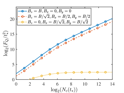
Figure S1: (Color online) The scaling relationships between the QFI and photon number $N_{c}$ are shown for different scenarios involving the estimated magnetic field $\vec{B}$: one where $\vec{B}$ is completely polarized in the $z$-axis direction (blue solid-line), another where it is partially polarized in the $z$-axis direction (red dashed-line), and and a third where it is perpendicular to the $z$-axis direction (yellow dotted-line). In these simulations, we use parameters consistent with those employed in the experiment by Bourhill16 : $\omega_{c}=\omega_{m}=15.506\times 2\pi$ GHZ, $g=7.11\times\pi$ GHZ, $\kappa_{c}=\kappa_{m}=1.029\times\pi$ MHZ. Additionally, the $t_{*}$ stands for the time corresponding to the point of maximum QFI and the thermal noise is given by $n_{c}=n_{m}=30$.

IV IV. QUantum Critical Dynamics (Beyond the RWA)

For the study of quantum critical dynamics, we consider the following Hamiltonian including the counter-rotating terms

$$\hat{H}=\omega_{c}\hat{c}^{\dagger}\hat{c}+\omega_{m}\hat{b}^{\dagger}\hat{b}+g(\hat{c}+\hat{c}^{\dagger})(\hat{b}+\hat{b}^{\dagger}).$$ (S46)

For $g<g_{c}=\sqrt{\omega_{m}\omega_{c}}/2$, the Hamiltonian (S46) can be rewritten in terms of two uncoupled bosonic modes Emary03 :

$$\hat{H}=\epsilon_{-}\hat{c}^{\dagger}_{1}\hat{c}_{1}+\epsilon_{+}\hat{c}^{\dagger}_{2}\hat{c}_{2},$$ (S47)

where $\epsilon_{\pm}^{2}=[\omega_{c}^{2}+\omega_{m}^{2}\pm\sqrt{(\omega_{c}^{2}-\omega_{m}^{2})^{2}+16g^{2}\omega_{c}\omega_{m}}]/2$ and the relations between bosons $\{\hat{c}_{1},\hat{c}_{2}\}$ and $\{\hat{c},\hat{b}\}$ are

$$\begin{bmatrix}\hat{c}\\ \hat{c}^{\dagger}\\ \hat{b}\\ \hat{b}^{\dagger}\end{bmatrix} = \frac{1}{2}\begin{bmatrix}\frac{\cos(\delta)}{\sqrt{\omega_{c}\epsilon_{-}}}(\omega_{c}+\epsilon_{-})&\frac{\cos(\delta)}{\sqrt{\omega_{c}\epsilon_{-}}}(\omega_{c}-\epsilon_{-})&\frac{\sin(\delta)}{\sqrt{\omega_{c}\epsilon_{+}}}(\omega_{c}+\epsilon_{+})&\frac{\sin(\delta)}{\sqrt{\omega_{c}\epsilon_{+}}}(\omega_{c}-\epsilon_{+})\\ \frac{\cos(\delta)}{\sqrt{\omega_{c}\epsilon_{-}}}(\omega_{c}-\epsilon_{-})&\frac{\cos(\delta)}{\sqrt{\omega_{c}\epsilon_{-}}}(\omega_{c}+\epsilon_{-})&\frac{\sin(\delta)}{\sqrt{\omega_{c}\epsilon_{+}}}(\omega_{c}-\epsilon_{+})&\frac{\sin(\delta)}{\sqrt{\omega_{c}\epsilon_{+}}}(\omega_{c}+\epsilon_{+})\\ \frac{-\sin(\delta)}{\sqrt{\omega_{0}\epsilon_{-}}}(\omega_{0}+\epsilon_{-})&\frac{-\sin(\delta)}{\sqrt{\omega_{0}\epsilon_{-}}}(\omega_{0}-\epsilon_{-})&\frac{\cos(\delta)}{\sqrt{\omega_{0}\epsilon_{+}}}(\omega_{0}+\epsilon_{+})&\frac{\cos(\delta)}{\sqrt{\omega_{0}\epsilon_{+}}}(\omega_{0}-\epsilon_{+})\\ \frac{-\sin(\delta)}{\sqrt{\omega_{0}\epsilon_{-}}}(\omega_{0}-\epsilon_{-})&\frac{-\sin(\delta)}{\sqrt{\omega_{0}\epsilon_{-}}}(\omega_{0}+\epsilon_{-})&\frac{\cos(\delta)}{\sqrt{\omega_{0}\epsilon_{+}}}(\omega_{0}-\epsilon_{+})&\frac{\cos(\delta)}{\sqrt{\omega_{0}\epsilon_{+}}}(\omega_{0}+\epsilon_{+})\\ \end{bmatrix}\begin{bmatrix}\hat{c}_{1}\\ \hat{c}_{1}^{\dagger}\\ \hat{c}_{2}\\ \hat{c}_{2}^{\dagger}\end{bmatrix}\equiv\hat{T}_{2}\begin{bmatrix}\hat{c}_{1}\\ \hat{c}_{1}^{\dagger}\\ \hat{c}_{2}\\ \hat{c}_{2}^{\dagger}\end{bmatrix}.$$ (S48)

Moreover, we define the operators $\hat{T}_{1}$, $\hat{T}_{3}(t)$ by

$$\begin{bmatrix}\hat{X}_{c}\\ \hat{P}_{c}\\ \hat{X}_{m}\\ \hat{P}_{m}\end{bmatrix} = \frac{1}{\sqrt{2}}\begin{bmatrix}1&1&0&0\\ -i&i&0&0\\ 0&0&1&1\\ 0&0&-i&i\\ \end{bmatrix}\begin{bmatrix}\hat{c}\\ \hat{c}^{\dagger}\\ \hat{b}\\ \hat{b}^{\dagger}\end{bmatrix}\equiv\hat{T}_{1}\begin{bmatrix}\hat{c}\\ \hat{c}^{\dagger}\\ \hat{b}\\ \hat{b}^{\dagger}\end{bmatrix},$$

$$\begin{bmatrix}\hat{c}_{1}(t)\\ \hat{c}_{1}^{\dagger}(t)\\ \hat{c}_{2}(t)\\ \hat{c}_{2}^{\dagger}(t)\end{bmatrix} = \begin{bmatrix}\exp(-i\epsilon_{-}t)&0&0&0\\ 0&\exp(i\epsilon_{-}t)&0&0\\ 0&0&\exp(-i\epsilon_{+}t)&0\\ 0&0&0&\exp(i\epsilon_{+}t)\\ \end{bmatrix}\equiv\hat{T}_{3}(t)\begin{bmatrix}\hat{c}_{1}(0)\\ \hat{c}_{1}^{\dagger}(0)\\ \hat{c}_{2}(0)\\ \hat{c}_{2}^{\dagger}(0)\end{bmatrix},$$ (S49)

where $\delta=\text{arctan}[4g\sqrt{\omega_{c}\omega_{m}}/(\omega_{m}^{2}-\omega_{c}^{2})]/2$. We consider the vacuum state as the initial state, i.e., $\gamma(0)=\mathds{1}_{4}$. By the formular $\gamma(t)=\hat{M}(t)\gamma(0)\hat{M}^{\dagger}(t)$ with $\hat{M}(t)=\hat{T}_{1}\hat{T}_{2}\hat{T}_{3}(t)\hat{T}_{2}^{-1}\hat{T}_{1}^{-1}$, we obtain the covariance matrix of the cavity state as follows

$$[\gamma^{c}(t)]_{11} = 1+\cos^{2}\delta(\cos^{2}\delta-1)(\omega_{c}-\omega_{m})\left(\frac{2}{\omega_{m}}[\cos(\epsilon_{+}t)\cos(\epsilon_{-}t)-1]-\frac{2\omega_{c}}{\epsilon_{+}\epsilon_{-}}\sin(\epsilon_{+}t)\sin(\epsilon_{-}t)\right)$$

$$-\frac{1}{2\epsilon_{+}^{2}\omega_{m}}(\cos^{2}\delta-1)\left[(\omega_{c}\omega_{m}+\epsilon_{+}^{2})(\omega_{c}-\omega_{m})\cos^{2}\delta+(\epsilon_{+}^{2}-\omega_{c}^{2})\omega_{m}\right]\left[\cos(2\epsilon_{+}t)-1\right]$$

$$-\frac{1}{2\epsilon_{-}^{2}\omega_{m}}\cos^{2}\delta\left[(\omega_{c}\omega_{m}+\epsilon_{-}^{2})(\omega_{c}-\omega_{m})\cos^{2}\delta+(\omega_{m}^{2}-\epsilon_{-}^{2})\omega_{c}\right]\left[\cos(2\epsilon_{-}t)-1\right],$$

$$\ [\gamma^{c}(t)]_{22} = 1-\cos^{2}\delta(\cos^{2}\delta-1)(\omega_{c}-\omega_{m})\left(\frac{2}{\omega_{c}}[\cos(\epsilon_{+}t)\cos(\epsilon_{-}t)-1]-\frac{2\epsilon_{+}\epsilon_{-}}{\omega_{c}^{2}\omega_{m}}\sin(\epsilon_{+}t)\sin(\epsilon_{-}t)\right)$$

$$+\frac{1}{2\omega_{c}^{2}\omega_{m}}(\cos^{2}\delta-1)\left[(\omega_{c}-\omega_{m})(\omega_{c}\omega_{m}+\epsilon_{+}^{2})\cos^{2}\delta+(\epsilon_{+}^{2}-\omega_{c}^{2})\omega_{m}\right]\left[\cos(2\epsilon_{+}t)-1\right]$$

$$+\frac{1}{2\omega_{c}^{2}\omega_{m}}\cos^{2}\delta\left[(\omega_{c}-\omega_{m})(\omega_{c}\omega_{m}+\epsilon_{-}^{2})\cos^{2}\delta-(\epsilon_{-}^{2}-\omega_{m}^{2})\omega_{c}\right]\left[\cos(2\epsilon_{-}t)-1\right],$$

$$\ [\gamma^{c}(t)]_{12} = -\cos^{2}\delta(\cos^{2}\delta-1)(\omega_{c}-\omega_{m})\left(\frac{\epsilon_{+}^{2}+\omega_{c}\omega_{m}}{\epsilon_{+}\omega_{c}\omega_{m}}\sin(\epsilon_{+}t)\cos(\epsilon_{-}t)+\frac{\epsilon_{-}^{2}+\omega_{c}\omega_{m}}{\epsilon_{-}\omega_{c}\omega_{m}}\cos(\epsilon_{+}t)\sin(\epsilon_{-}t)\right)$$ (S50)

$$+\frac{1}{2\epsilon_{+}\omega_{c}\omega_{m}}(\cos^{2}\delta-1)\left[\cos^{2}\delta(\omega_{c}-\omega_{m})(\epsilon_{+}^{2}+\omega_{c}\omega_{m})+(\epsilon_{+}^{2}-\omega_{c}^{2})\omega_{m}\right]\sin(2\epsilon_{+}t)$$

$$+\frac{1}{2\epsilon_{-}\omega_{c}\omega_{m}}\cos^{2}\delta\left[\cos^{2}\delta(\omega_{c}-\omega_{m})(\epsilon_{-}^{2}+\omega_{c}\omega_{m})-(\epsilon_{-}^{2}-\omega_{m}^{2})\omega_{c}\right]\sin(2\epsilon_{-}t).$$

Notice that $\cos^{2}\delta\neq 0,1$, $\epsilon_{-}=\sqrt{\frac{\omega_{c}^{2}+\omega_{m}^{2}}{2}\left(1-\sqrt{1+\frac{16\omega_{c}\omega_{m}}{(\omega_{c}^{2}+\omega_{m}^{2})^{2}}(g^{2}-g_{c}^{2})}\right)}\sim(g_{c}-g)^{1/2}\to 0$ as $g\to g_{c}$ but $\epsilon_{+}$ is finite. Thus from Eq. (IV) we see that the finiteness of the covariance matrix $\gamma^{c}(t)$ requires $\sin(\epsilon_{-}t)=0$. We denote such a time $t$ as $t_{*}:=n\pi/\epsilon_{-}$, $n\in\mathbb{Z}_{>0}$. For time $t_{*}$ we deduce from Eq. (IV) that the divergence of $[\gamma^{c}(t_{*})]^{\prime}$ behaves as follows

$$[\gamma^{c}(t_{*})]_{11}^{\prime}\sim\left.\left[\frac{\sin(\epsilon_{-}t)}{\epsilon_{-}}\right]^{\prime}\right|_{t=t_{*}}\sim\frac{\epsilon_{-}^{\prime}}{\epsilon}t_{*}\sim(g_{c}-g)^{-1}t_{*},$$

$$[\gamma^{c}(t_{*})]^{\prime}_{22}\sim(g_{c}-g)^{0}t_{*},$$

$$[\gamma^{c}(t_{*})]^{\prime}_{12}\sim\left.\left[\frac{\sin(\epsilon_{-}t)}{\epsilon_{-}}\right]^{\prime}\right|_{t=t_{*}}\sim\frac{\epsilon_{-}^{\prime}}{\epsilon}t_{*}\sim(g_{c}-g)^{-1}t_{*},$$ (S51)

when $g\to g_{c}$. Here we have used the result that $\epsilon^{\prime}_{-}\sim(g_{c}-g)^{-1/2}$ and $\epsilon_{-}\sim(g_{c}-g)^{1/2}$ as $g\to g_{c}$. Substituting Eq. (IV) into Eq. (S12) we obtain

$$n^{\prime}_{\rm th}=\frac{\det^{\prime}(\gamma^{c})}{4\sqrt{\det(\gamma^{c})}}\sim(g_{c}-g)^{-1}t_{*},$$

$$\phi^{\prime}=\frac{1}{\left(\frac{2\gamma^{c}_{12}}{\gamma^{c}_{11}-\gamma^{c}_{22}}\right)^{2}+1}\frac{2(\gamma^{c}_{12})^{\prime}(\gamma^{c}_{11}-\gamma^{c}_{22})-2\gamma^{c}_{12}[\gamma^{c}_{11}-\gamma^{c}_{22}]^{\prime}}{(\gamma^{c}_{11}-\gamma^{c}_{22})^{2}}\sim(g_{c}-g)^{-1}t_{*},$$

$$r^{\prime}=\frac{1}{2\sqrt{\left(\frac{\mathrm{Tr}(\gamma^{c})}{2\sqrt{\det(\gamma^{c})}}\right)^{2}-1}}\frac{2\sqrt{\det(\gamma^{c})}\mathrm{Tr}^{\prime}(\gamma^{c})-\det^{\prime}(\gamma^{c})\mathrm{Tr}(\gamma^{c})/\sqrt{\det(\gamma^{c})}}{4\det(\gamma^{c})}\sim(g_{c}-g)^{-1}t_{*}.$$ (S52)

Since the covariance matrix $\gamma^{c}(t_{*})$ is finite then the criticality contribution to QFI and CFI both comes from the divergence of $r^{\prime}$, $\phi^{\prime}$ and $n^{\prime}_{\rm th}$. By substituting Eq. (IV) into Eqs. (S21) and (S30) we obtain the scalings of QFI and CFI at time $t_{*}\sim(g_{c}-g)^{-1/2}$ as follows

$$F_{Q}(t_{*})\sim(g_{c}-g)^{-2}t_{*}^{2},$$

$$F_{C}(t_{*})\sim(g_{c}-g)^{-2}t_{*}^{2}.$$ (S53)

For $t\neq t_{*}$, the covariance matrix $\gamma^{c}$ is no longer finite but divergent as $g\to g_{c}$. According to Eq. (IV) we obtain

$$[\gamma^{c}(t)]_{11}\sim\frac{1}{\epsilon_{-}^{2}}\sim(g_{c}-g)^{-1}$$

$$[\gamma^{c}(t)]_{22}\sim(g_{c}-g)^{0}$$

$$[\gamma^{c}(t)]_{12}\sim\frac{1}{\epsilon_{-}}\sim(g_{c}-g)^{-1/2},$$ (S54)

where $t\neq t_{*}$. We further require that the time $t$ scales as $(g_{c}-g)^{-1/2}$ and makes $[\gamma^{c}(t)]^{\prime}$ achieving its maximum divergence. That is to say,

$$[\gamma^{c}(t)]_{11}^{\prime}\sim\left[\frac{\cos(2\epsilon_{-}t)}{\epsilon_{-}^{2}}\right]^{\prime}\sim(g_{c}-g)^{-3/2}t,$$

$$[\gamma^{c}(t)]_{22}^{\prime}\sim(g_{c}-g)^{0}t$$

$$[\gamma^{c}(t)]_{12}^{\prime}\sim\left[\frac{\sin(\epsilon_{-}t)}{\epsilon_{-}}\right]^{\prime}\sim(g_{c}-g)^{-1}t,$$ (S55)

which can be realized by choosing $t=t_{*}/4=\pi/(4\epsilon_{-})$. Substituting Eqs. (IV) and (IV) into Eq. (S12) we obtain

$$n_{\rm th}=\frac{\sqrt{\det(\gamma^{c})}-1}{2}\sim(g_{c}-g)^{-1/2},$$

$$\cosh(2r)=\frac{\mathrm{Tr}(\gamma^{c})}{2\sqrt{\det(\gamma^{c})}}\sim(g_{c}-g)^{-1/2},$$

$$n^{\prime}_{\rm th}=\frac{\det^{\prime}(\gamma^{c})}{4\sqrt{\det(\gamma^{c})}}\sim(g_{c}-g)^{-1}t_{*},$$

$$\phi^{\prime}=\frac{1}{\left(\frac{2\gamma^{c}_{12}}{\gamma^{c}_{11}-\gamma^{c}_{22}}\right)^{2}+1}\frac{2(\gamma^{c}_{12})^{\prime}(\gamma^{c}_{11}-\gamma^{c}_{22})-2\gamma^{c}_{12}[\gamma^{c}_{11}-\gamma^{c}_{22}]^{\prime}}{(\gamma^{c}_{11}-\gamma^{c}_{22})^{2}}\sim(g_{c}-g)^{0}t_{*},$$

$$r^{\prime}=\frac{1}{2\sqrt{\left(\frac{\mathrm{Tr}(\gamma^{c})}{2\sqrt{\det(\gamma^{c})}}\right)^{2}-1}}\frac{2\sqrt{\det(\gamma^{c})}\mathrm{Tr}^{\prime}(\gamma^{c})-\det^{\prime}(\gamma^{c})\mathrm{Tr}(\gamma^{c})/\sqrt{\det(\gamma^{c})}}{4\det(\gamma^{c})}\sim(g_{c}-g)^{-1/2}t_{*}.$$ (S56)

Thus, by Eqs. (S21) and (S30), we obtain the maximum scaling of QFI and CFI

$$F_{Q}(t_{*}/4)\sim(g_{c}-g)^{-1}t_{*}^{2},$$

$$F_{C}(t_{*}/4)\sim(g_{c}-g)^{-1}t_{*}^{2},$$ (S57)

when $t=t_{*}/4=\pi/(4\epsilon_{-})$.

References

(1)
C. M. Caves, K. S. Thorne, R. W. P. Drever, V. D. Sand- berg, and M. Zimmermann, On the measurement of a weak classical force coupled to a quantum-mechanical oscillator. I. Issues of principle,
Rev. Mod. Phys. 52, 341 (1980).
(3)
L. Pezzé, A. Smerzi, M. K. Oberthaler, R. Schmied, and P. Treutlein, Quantum metrology with nonclassical states of atomic ensembles,
Rev. Mod. Phys. 90, 035005 (2018).
(5)
P. Hyllus, W. Laskowski, R. Krischek, C. Schwemmer, W. Wieczorek, H. Weinfurter, L. Pezzé, and A. Smerzi, Fisher information and multiparticle entanglement,
Phys. Rev. A 85, 022321 (2012).
(8)
Z. Ren, W. Li, A. Smerzi, and M. Gessner,
Metrological Detection of Multipartite Entanglement from Young Diagrams,
Phys. Rev. Lett. 126, 080502 (2021).
(9)
Y. Su and X. Wang, Parametrized protocol achieving the Heisenberg limit in the optical domain via dispersive atom-light interactions,
Results Phys. 24, 104159 (2021).
(10)
B. Yadin, M. Fadel, and M. Gessner, Metrological com- plementarity reveals the EinsteinPodolsky-Rosen paradox,
Nat. Commun. 12, 2410 (2021); Author Correction: Metrological complementarity reveals the Einstein-Podolsky-Rosen paradox, Nat Commun 12, 6481 (2021).
(11)
F. Fröwis, M. Fadel, P. Treutlein, N. Gisin, and N. Brunner,Does large quantum Fisher information imply Bell correlations?
Phys. Rev. A 99, 040101(R) (2019).
(12)
I. Gianani, V. Berardi, and M. Barbieri, Witnessing quantum steering by means of the Fisher information,
Phys. Rev. A 105, 022421 (2022)
.
(13)
A. Niezgoda and J. Chwedenćzuk, Many-Body Nonlocality as a Resource for Quantum-Enhanced Metrology, Phys. Rev. Lett. 126, 210506 (2021).
(14)
D. Girolami, A. M. Souza, V. Giovannetti, T. Tufarelli, J. G. Filgueiras, R. S. Sarthour, D. O. Soares-Pinto, I. S. Oliveira, and G. Adesso,
Quantum Discord Determines the Interferometric Power of Quantum States,
Phys. Rev. Lett. 112, 210401 (2014).
(16)
A. Sone, Q. Zhuang, C. Li, Y.-X. Liu, and P. Cappellaro, Nonclassical correlations for quantum metrology in thermal equilibrium,
Phys. Rev. A 99, 052318 (2019).
(17)
P. Jurcevic, B. P. Lanyon, P. Hauke, C. Hempel, P. Zoller, R. Blatt, and C. F. Roos, Quasiparticle engineering and entanglement propagation in a quantum many-body system,
Nature 511, 202 (2014).
(18)
O. A. Castro-Alvaredo, C. De Fazio, B. Doyon, and I. M. Szécsényi, Entanglement Content of Quasiparticle Excitations, Phys. Rev. Lett. 121, 170602 (2018).
(19)
N. Laflorencie, Quantum entanglement in condensed matter systems, Phys. Rep. 646, 1 (2016).
(20)
L. Venema, B. Verberck, I. Georgescu, G. Prando, E. Couderc, S. Milana, M. Maragkou, L. Persechini, G. Pacchioni, and L. Fleet, The quasiparticle zoo, Nature Phys. 12, 1085 (2016).
(26)
V. Scarani04, N. Gisin, and S. Popescu, Proposal for Energy-Time Entanglement of Quasiparticles in a Solid-State Device, Phys. Rev. Lett. 92, 167901 (2004).
(33)
L. Garbe, M. Bina, A. Keller, M. G. A. Paris, and S. Felicetti, Critical Quantum Metrology with a Finite-Component Quantum Phase Transition, Phys. Rev. Lett. 124, 120504 (2020).
(34)
V. Montenegro, U. Mishra, and A. Bayat, Global Sensing and Its Impact for Quantum Many-Body Probes with Criticality, Phys. Rev. Lett. 126, 200501 (2021).
(36)
R. Liu, Y. Chen, M. Jiang, X. Yang, Z. Wu, Y. Li, H. Yuan, X. Peng, and J. Du, Experimental critical quantum metrology with the Heisenberg scaling, npj Quantum Inf. 7, 170 (2021).
(37)
T. Ilias, D. Yang, S. F. Huelga, and M. B. Plenio, Criticality-Enhanced Quantum Sensing via Continuous Measurement, PRX Quantum 3, 010354 (2022).
(38)
D. Yang, S. F. Huelga, and M. B. Plenio, Efficient Information Retrieval for Sensing via Continuous Measurement, Phys. Rev. X 13, 031012 (2023).
(39)
R. Di Candia, F. Minganti, K. V. Petrovnin, G. S. Paraoanu, and S. Felicetti, Critical parametric quantum sensing, npj Quantum Inf 9, 23 (2023).
(40)
P. Krammer, H. Kampermann, D. Bruß, R. A. Bertlmann, L. C. Kwek, and C. Macchiavello, Multipartite Entanglement Detection via Structure Factors,
Phys. Rev. Lett. 103, 100502 (2009).
(41)
P. Hauke, M. Heyl, L. Tagliacozzo, and P. Zoller, Measuring multipartite entanglement through dynamic susceptibilities,
Nature Phys. 12, 778 (2016).
(42)
A. V. Chumak, V. I. Vasyuchka, A. A. Serga, B. Hillebrands, Magnon spintronics, Nature Phys. 11, 453 (2015).
(43)
B. Lenk, H. Ulrichs, F. Garbs, and M. Münzenberg, The building blocks of magnonics, Phys. Rep. 507, 107 (2011).
(44)
H.Y. Yuan, Y. Cao, A. Kamra, R. A. Duine, and P. Yan, Quantum magnonics: When magnon spintronics meets quantum information science, Phys. Rep. 965, 1 (2022).
(45)
B. Z. Rameshti, S. V. Kusminskiy, J. A. Haigh, K. Usami,
D. Lachance-Quirion, Y. Nakamura, C.-M. Hu, H. X. Tang,
G. E. W. Bauer, and Y. M. Blanter, Cavity magnonics,
Phys.
Rep. 979, 1 (2022).
(46)
Y. Li, W. Zhang, V. Tyberkevych, W.-K. Kwok, A. Hoffmann, and V. Novosad, Hybrid magnonics: Physics, circuits, and applications for coherent information processing, J. Appl. Phys. 128, 130902 (2020).
(50)
M. Yu, H. Shen, and J. Li, Magnetostrictively Induced Stationary Entanglement between Two Microwave Fields, Phys. Rev. Lett. 124, 213604 (2020).
(51)
H. Y. Yuan, P. Yan, S. Zheng, Q. Y. He, K. Xia, and M.-H. Yung, Steady Bell State Generation via Magnon-Photon Coupling, Phys. Rev. Lett. 124, 053602 (2020).
(52)
H. Huebl, C. W. Zollitsch, J. Lotze, F. Hocke, M. Greifenstein, A. Marx, R. Gross, and S. T. B. Goennenwein, High Cooperativity in Coupled Microwave Resonator Ferrimagnetic Insulator Hybrids, Phys. Rev. Lett. 111, 127003 (2013).
(53)
D. Lachance-Quirion, S. P. Wolski, Y. Tabuchi, S. Kono, K.
Usami, and Y. Nakamura, Entanglement-based single-shot
detection of a single magnon with a superconducting qubit,
Science 367, 425 (2020).
(54)
S. P. Wolski, D. Lachance-Quirion, Y. Tabuchi, S. Kono, A. Noguchi, K. Usami, and Y. Nakamura, Dissipation-Based Quantum Sensing of Magnons with a Superconducting Qubit, Phys. Rev. Lett. 125, 117701 (2020).
(55)
Ö. O. Soykal and M. E. Flatté, Strong Field Interactions between a Nanomagnet and a Photonic Cavity, Phys. Rev. Lett. 104, 077202 (2010).
(56)
M. Elyasi, Y. M. Blanter, and G. E. W. Bauer, Resources of nonlinear cavity magnonics for quantum information, Phys. Rev. B 101, 054402 (2020).
(57)
Z. Zhang, M. O. Scully, and G. S. Agarwal, Quantum entanglement between two magnon modes via Kerr nonlinearity driven far from equilibrium, Phys. Rev. Research 1, 023021 (2019).
(58)
V. A. Mousolou, Y. Liu, A. Bergman, A. Delin, O. Eriksson, M. Pereiro, D. Thonig, and E. Sjöqvist, Magnon-magnon entanglement and its quantification via a microwave cavity, Phys. Rev. B 104, 224302 (2021).
(59)
H. Y. Yuan, S. Zheng, Z. Ficek, Q. Y. He, and M.-H. Yung, Enhancement of magnon-magnon entanglement inside a cavity, Phys. Rev. B 101, 014419 (2020).
(60)
G. M. Andolina, M. Keck, A. Mari, M. Campisi, V. Giovannetti, and M. Polini,
Extractable Work, the Role of Correlations, and Asymptotic Freedom in Quantum Batteries,
Phys. Rev. Lett. 122, 047702 (2019).
(61)
J.-X. Liu, H.-L. Shi, Y.-H. Shi, X.-H. Wang, and W.-L. Yang, Entanglement and work extraction in the central-spin quantum battery, Phys. Rev. B 104, 245418 (2021).
(62)
H.-L. Shi, S. Ding, Q.-K. Wan, X.-H. Wang, and W.-L. Yang, Entanglement, Coherence, and Extractable Work in Quantum Batteries, Phys. Rev. Lett. 129, 130602 (2022).
(63)
V. Montenegro, M. G. Genoni, A. Bayat, and M. G. A. Paris, Probing of nonlinear hybrid optomechanical systems via partial accessibility, Phys. Rev. Research 4, 033036 (2022).
(64)
V. Montenegro, M. G. Genoni, A. Bayat, and M. G. A. Paris, Mechanical oscillator thermometry in the nonlinear optomechanical regime, Phys. Rev. Research 2, 043338 (2020).
(65)
Y. Tabuchi, S. Ishino, T. Ishikawa, R. Yamazaki, K. Usami, and Y. Nakamura, Hybridizing Ferromagnetic Magnons and Microwave Photons in the Quantum Limit, Phys. Rev. Lett. 113, 083603 (2014).
(66)
X. Zhang, C.-L. Zou, L. Jiang, and H. X. Tang, Strongly Coupled Magnons and Cavity Microwave Photons, Phys. Rev. Lett. 113, 156401 (2014).
(67)
Ö. O. Soykal, and M. E. Flatté, Size dependence of strong coupling between nanomagnets and photonic cavities, Phys. Rev. B 82, 104413 (2010).
(68)
J. Bourhill, N. Kostylev, M. Goryachev, D. L. Creedon, and M. E. Tobar, Ultrahigh cooperativity interactions between magnons and resonant photons in a YIG sphere, Phys. Rev. B 93, 144420 (2016).
(69)
T. Holstein and H. Primakoff, Field Dependence of the Intrinsic Domain Magnetization of a Ferromagnet, Phys. Rev. 58, 1098 (1940).
(70)
This Hamiltonian is similar to the the one considered in
S. Kotler, A. Peterson, E. Shojaee, F. Lecocq, K. Cicak, A. Kwiatkowski, S. Geller, S. Glancy, E. Knill, R. W. Simmonds, J. Aumentado, and J. D. Teufel, Direct observation of deterministic macroscopic entanglement, Science 372, 622 (2021) and
L. Mercier de Lépinay, C. F. Ockeloen-Korppi, M. J. Woolley, and M. A. Sillanpää, Quantum mechanics-free subsystem with mechanical oscillators, Science 372, 625 (2021).
(71)
C. Emary and T. Brandes, Chaos and the quantum phase transition in the Dicke model, Phys. Rev. E 67, 066203 (2003).
(76)
Here, is the displacement operator,
is the squeezing operator with ,
and is a thermal state with and is the Fock state.
(77)
G. Adam, Density Matrix Elements and Moments for Generalized Gaussian State Fields, J. Mod. Opt. 42, 1311 (1995).
(78)
The expression of the quantum Fisher information for general Gaussian states has been obtain in terms of the covariance matrix and the displacement vector:
O. Pinel, P. Jian, N. Treps, C. Fabre, and D. Braun, Quantum parameter estimation using general single-mode Gaussian states, Phys. Rev. A 88, 040102(R) (2013)
;
A. Monras, Phase space formalism for quantum estimation of Gaussian states, arXiv:1303.3682.
(85)
K. McKenzie, D. A. Shaddock, D. E. McClelland, B. C.
Buchler, and P. K. Lam, Experimental Demonstration of a Squeezing-Enhanced Power-Recycled Michelson Interferometer for Gravitational Wave Detection, Phys. Rev. Lett. 88, 231102
(2002).
(86)
K. McKenzie, N. Grosse, W. P. Bowen, S. E. Whitcomb,
M. B. Gray, D. E. McClelland, and P. K. Lam, Squeezing in the Audio Gravitational-Wave Detection Band, Phys. Rev.
Lett. 93, 161105 (2004).
(87)
H. Vahlbruch, S. Chelkowski, B. Hage, A. Franzen,
K. Danzmann, and R. Schnabel, Demonstration of a Squeezed-Light-Enhanced Power- and Signal-Recycled Michelson Interferometer, Phys. Rev. Lett. 95,
211102 (2005).
(88)
H. Vahlbruch, S. Chelkowski, B. Hage, A. Franzen,
K. Danzmann, and R. Schnabel, Coherent Control of Vacuum Squeezing in the Gravitational-Wave Detection Band, Phys. Rev. Lett. 97,
011101 (2006).
(89)
The number of photons is given by .
The quantum squeezing-induced contribution to the number of photons is .
If we further consider the impact of thermalization, we can assume , analogous to the quantum squeezing-induced contribution.
The exact solution of the quantum dynamics governed by the Hamiltonian (S31) also confirmed this assumption, see Supplemental Material SM .
(91)
G. S. Agarwal, Entropy, the Wigner Distribution Function, and the Approach to Equilibrium of a System of Coupled Harmonic Oscillators, Phys. Rev. A 3, 828 (1971).
(93)
R. J. Rossi, Mathematical statistics: an introduction to likelihood based inference (John Wiley & Sons, New York, 2018).
(94)
C. Weedbrook, S. Pirandola, R. García-Patrón, N. J. Cerf, T. C. Ralph, J. H. Shapiro, and S. Lloyd, Gaussian quantum information, Rev. Mod. Phys. 84, 621 (2012).
(95)
G. Giedke and J. I. Cirac, Characterization of Gaussian operations and distillation of Gaussian states, Phys. Rev. A 66, 032316 (2002).
(96)
J. Eisert and M. B. Plenio, Introduction to the basics of entanglement theory in continuous-variable systems, Int. J. Quantum. Inform. 1, 479 (2003).
(97)
J. Li, S.-Y. Zhu, and G. S. Agarwal, Squeezed states of magnons and phonons in cavity magnomechanics, Phys. Rev. A 99, 021801(R) (2019).
(98)
S. O. Demokritov, V. E. Demidov, O. Dzyapko, G. A. Melkov, A. A. Serga, B. Hillebrands, and A. N. Slavin, Bose-Einstein condensation of quasi-equilibrium magnons at room temperature under pumping, Nature 443, 430-433 (2006).
(99)
W. Zhang, D.-Y. Wang, C.-H. Bai, T. Wang, S. Zhang, and H.-F. Wang, Generation and transfer of squeezed states in a cavity magnomechanical system by two-tone microwave fields, Opt. Express 29, 11773 (2021).
(101)
G. Wu, Y. Cheng, S. Guo, F. Yang, D. V. Pelekhov, and P. C. Hammel, Nanoscale imaging of Gilbert damping using signal amplitude mapping, Appl. Phys. Lett. 118, 042403 (2021).
(102) Here the scalings of the thermalization and squeezing parameters are explicitly given by
for and
for .
Details can be found in Supplemental Material.
Entanglement is positively related to .
(103)
M. Silaev, Ultrastrong magnon-photon coupling and entanglement in superconductor/ferromagnet nanostructures, arXiv:2211.00462.
(104)
J. W. Rao, B. Yao, C. Y. Wang, C. Zhang, T. Yu, and W. Lu, Unveiling a Pump-Induced Magnon Mode via Its Strong Interaction with Walker Modes, Phys. Rev. Lett. 130, 046705 (2023).
(105)
I. A. Golovchanskiy, N. N. Abramov, V. S. Stolyarov, A. A. Golubov, M. Yu. Kupriyanov, V.V. Ryazanov, and A.V. Ustinov, Approaching Deep-Strong On-Chip Photon-To-Magnon Coupling, Phys. Rev. Applied 16, 034029 2021).
(106)
A. F. Kockum, A. Miranowicz, S. De Liberato, S. Savasta, and F. Nori, Ultrastrong coupling between light and matter, Nat. Rev. Phys. 1, 19-40 (2019).
(107)
I. Boventer, M. Pfirrmann, J. Krause, Y. Schön, M. Kläui, and M. Weides, Complex temperature dependence of coupling and dissipation of cavity magnon polaritons from millikelvin to room temperature,
Phys. Rev. B 97, 184420 (2018).
(108)
I. A. Golovchanskiy, N. N. Abramov, V. S. Stolyarov, et al. Ultrastrong photon-to-magnon coupling in multilayered heterostructures involving superconducting coherence via ferromagnetic layers, Sci. Adv. 7, eabe8638 (2021).
(109)
N. Kostylev, M. Goryachev, M. E. Tobar, Superstrong coupling of a microwave cavity to yttrium iron garnet magnons, Appl. Phys. Lett. 108, 062402 (2016).
(110)
D. Xu, X.-K. Gu, H.-K. Li, Y.-C. Weng, Y.-P. Wang, J. Li, H. Wang, S.-Y. Zhu, and J. Q. You, Quantum Control of a Single Magnon in a Macroscopic Spin System, Phys. Rev. Lett. 130, 193603 (2023).