Provable Multi-instance Deep AUC Maximization with Stochastic Pooling

Abstract

This paper considers a novel application of deep AUC maximization (DAM) for multi-instance learning (MIL), in which a single class label is assigned to a bag of instances (e.g., multiple 2D slices of a CT scan for a patient). We address a neglected yet non-negligible computational challenge of MIL in the context of DAM, i.e., bag size is too large to be loaded into GPU memory for backpropagation, which is required by the standard pooling methods of MIL. To tackle this challenge, we propose variance-reduced stochastic pooling methods in the spirit of stochastic optimization by formulating the loss function over the pooled prediction as a multi-level compositional function. By synthesizing techniques from stochastic compositional optimization and non-convex min-max optimization, we propose a unified and provable muli-instance DAM (MIDAM) algorithm with stochastic smoothed-max pooling or stochastic attention-based pooling, which only samples a few instances for each bag to compute a stochastic gradient estimator and to update the model parameter. We establish a similar convergence rate of the proposed MIDAM algorithm as the state-of-the-art DAM algorithms. Our extensive experiments on conventional MIL datasets and medical datasets demonstrate the superiority of our MIDAM algorithm. The method is open-sourced at https://libauc.org/.

1 Introduction

Deep AUC maximization (DAM) has recently achieved great success for many AI applications due to its capability of handling imbalanced data (Yang & Ying, 2022). For example, it earned first place at Stanford CheXpert competition (Irvin et al., 2019), and state-of-the-art performance on other datasets (Yuan et al., 2021; Wang et al., 2021b). However, a novel application of DAM for multi-instance learning (MIL) has not been studied in the literature.

MIL refers to a setting where multiple instances are observed for an object of interest and only one label is given to describe that object. Many real-life applications can be formulated as MIL. For example, the medical imaging data for diagnosing a patient usually consists of a series of 2D high-resolution images (e.g., CT scan), and only a single label (containing a tumor or not) is assigned to the patient (Quellec et al., 2017). MIL has a long history in machine learning and various methods have been proposed for traditional learning with tabular data (Babenko, 2008; Carbonneau et al., 2016) and deep learning (DL) with unstructured data (Oquab et al., 2015; Charles et al., 2017; Ilse et al., 2018). The fundamental theorem of symmetric functions (Zaheer et al., 2017; Qi et al., 2016), inspires a general three-step approach for classifying a bag of instances: (i) a transformation of individual instances, (ii) a pooling of transformed instances using a symmetric (permutation-invariant) function, (iii) a transformation of pooled representation. A key in the implementation of the three steps is the symmetric function that takes the transformations of all instances as input and produces an output, which is also known as the pooling operation. In the literature, various pooling strategies have been explored, e.g., max pooling, average pooling, and smoothed-max (i.e., log-exp-sum) pooling of predictions (Ramon et al., 2000), attention-based pooling of feature representations (Ilse et al., 2018).

However, to the best of our knowledge, none of the existing works have tackled the computational challenge of MIL in the context of DL when a bag is large due to the existence of multiple instances in the bag. The limitation of computing resources (e.g., the memory size of GPU) might prevent loading all instances of a bag at once, creating a severe computational bottleneck for training. For example, an MRI scan of the brain may produce up to hundreds of 2D slices of high resolution (Calabrese et al., 2022). It is hard to process all slices of a patient at each iteration for DL. Even if the size of an image can be reduced to fit into the memory, the convergence performance will be compromised due to a small batch size (i.e., few patients can be processed due to many slices per patient). A naive approach to deal with this challenge is to use mini-batch stochastic pooling, i.e., only sampling a few instances from a bag for computing the pooled prediction and conducting the update. However, this naive approach does not ensure optimization of the objective that is defined using the pooling of all instances for each bag due to the error of mini-batch stochastic pooling.

We tackle this challenge of multi-instance DAM in a spirit of stochastic optimization by (i) formulating the pooled prediction as a compositional function whose inner functions are expected functions over instances of that bag, and (ii) proposing efficient and provable stochastic algorithms for solving the non-convex min-max optimization with a multi-level compositional objective function. A key feature of the proposed algorithms is replacing the deterministic pooling over all instances of a bag by a variance-reduced stochastic pooling (VRSP), whose computation only requires sampling a few instances from the bag. To ensure the optimization of the original objective, the VRSP is constructed following the principle of stochastic compositional optimization such that the variance of stochastic pooling estimators is reduced in the long term. In particular, the inner functions of the pooled prediction are tracked and estimated by moving average estimators separately for each bag. Based on VRSP, stochastic gradient estimators are computed for updating the model parameter, which can be efficiently implemented by backpropagation.

Our contributions are summarized in the following:

• We propose variance-reduced stochastic pooling estimators for both smoothed-max pooling and attention-based pooling. Building on these stochastic pooling estimators, we develop unified efficient algorithms of multi-instance DAM (MIDAM) based on a min-max objective for the two pooling operations.

• We develop novel convergence analysis of the proposed MIDAM algorithms by (i) proving the averaged error of variance-reduced stochastic pooling estimators over all iterations will converge to zero, and (ii) establishing a convergence rate showing our algorithms can successfully find an $\epsilon$-stationary solution of the min-max objective of DAM.

• We conduct extensive experiments of proposed MIDAM algorithms on conventional MIL benchmark datasets and emerging medical imaging datasets with high-resolution medical images, demonstrating the better performance of our algorithms.

2 Related Works

In this section, we introduce previous works on AUC maximization, multi-instance learning, and medical image classification, and then discuss how they are related to our work.

Deep AUC maximization (DAM). Maximizing the area under the receiver operating characteristic curve (AUC), as an effective method for dealing with imbalanced datasets, has been vigorously studied for the last two decades (Yang & Ying, 2022). Earlier studies focus on learning traditional models, e.g., SVM, decision tree (Cortes & Mohri, 2003; Joachims, 2005b; Ferri et al., 2002). Inspired by the Wilcoxon-Man-Whitney statistic, a variety of pairwise losses and optimization algorithms have been studied for AUC optimization (Gao et al., 2013; Zhao et al., 2011a; Kotlowski et al., 2011; Gao & Zhou, 2015; Calders & Jaroszewicz, 2007; Charoenphakdee et al., 2019). Inspired by the min-max objective corresponding to the pairwise square loss function (Ying et al., 2016), stochastic algorithms have been developed for DAM (Liu et al., 2020; Yuan et al., 2021). In this work, we propose efficient and scalable methods for DAM under the multi-instance learning (MIL) scenario with real big-data applications.

Multi-instance learning. Multi-instance learning (MIL) has been extensively studied and adopted for real applications since decades ago (Ramon & De Raedt, 2000; Andrews et al., 2002; Oquab et al., 2015; Kraus et al., 2016). Usually, a simple MIL pooling strategy, that is, max-pooling over a data bag has been widely utilized. This idea has been incorporated with support vector machine (SVM) and neural networks (Andrews et al., 2002; Oquab et al., 2015; Wang, 2018). Other pooling strategies have also been proposed, e.g., mean, smoothed-max (aka. log-sum-exponential), generalized mean, noisy-or, noisy-and (Wang, 2018; Ramon & De Raedt, 2000; Keeler et al., 1990; Kraus et al., 2016). Recently, attention-based pooling was proposed for deep MIL (Ilse et al., 2018). It is worth noting that almost all the pooling strategies (except max-pooling) require loading all the data from a bag to do the computation, specifically backpropagation. However, there is still no existing method that considers mitigating the computational issue when the data size is too large even for a single data bag.

Medical image classification. In MRI/CT scans, multiple slices of images are acquired at different locations of the patient?s body, which not only improves the diagnostic capabilities but also lowers doses of radiation. Hence, a patient can be represented by a series of 2D slices. A traditional approach is to concatenate these 2D slices into a 3D image and then learn a 3D convolutional neural network (CNN) (Singh et al., 2020). However, this approach suffers from several drawbacks. First, it demands more computational and memory resources as processing high-resolution 3D images is more costly than processing 2D images. As a consequence, the mini-batch size for back-propagation in training is compromised or the resolution is reduced, which can harm the learning capability. Third, it is more difficult to interpret the prediction of a DL model based on 3D images as radiologists still use 2D slices to make diagnostic decision (Brunyé et al., 2020). To avoid these issues, we will investigate MIL and make it practical for medical image classification.

3 Preliminaries

Notations. Let $\mathcal{X}_{i}=\{\mathbf{x}_{i}^{1},\ldots,\mathbf{x}_{i}^{n_{i}}\}$ denote a bag of data instances (e.g., 2D image slices of an MRI/CT scan). Let $\mathcal{D}=\{(\mathcal{X}_{i},y_{i}),i=1,\ldots,n\}$ denote the set of labeled data, where $y_{i}\in\{0,1\}$ denotes the label associated with the bag $i$. Let $\mathcal{D}_{+}\subset\mathcal{D}$ only contain $D_{+}$ positive bags with $y_{i}=1$ and $\mathcal{D}_{-}\subset\mathcal{D}$ only contain $D_{-}$ negative bags with $y_{i}=0$. Without loss of generality, let $\mathbf{w}\in\mathbb{R}^{d}$ denote all weights to be learned, which includes the weights of the feature encoder network, the weights of the instance-level classifier, and the parameters in the attention-based pooling. Let $e(\mathbf{w}_{e};\mathbf{x})\in\mathbb{R}^{d_{o}}$ be the instance-level representation encoded by a neural network $\mathbf{w}_{e}$, $\phi(\mathbf{w};\mathbf{x})\in[0,1]$ be the instance-level prediction score (after some activation function), and $h(\mathbf{w};\mathcal{X}_{i})\in[0,1]$ be the pooled prediction score of the bag $i$ over all its instances. Besides, $\sigma(\cdot)$ denotes the sigmoid activation.

Multi-instance Learning (MIL). We work under the standard MIL assumption that (i) an instance can be associated with a label and (ii) a bag is labeled positive if at least one of its instances has a positive label, and negative if all of its instances have negative labels (Dietterich et al., 1997b). The assumption implies that a MIL model must be permutation-invariant for the prediction function $h(\mathcal{X})$. To achieve permutation invariant property, fundamental theorems of symmetric functions have been developed (Zaheer et al., 2017; Qi et al., 2016). In particular, Zaheer et al. (2017) show that a scoring function for a set of instances $\mathcal{X}$, $h(\mathcal{X})\in\mathbb{R}$, is a symmetric function if and only if it can be decomposed as $h(\mathcal{X})=g(\sum_{\mathbf{x}\in\mathcal{X}}\psi(\mathbf{x}))$, where $g$ and $\psi$ are suitable transformations. Qi et al. (2016) prove that for any $\epsilon>0$, a Hausdorff continuous symmetric function $h(\mathcal{X})\in\mathbb{R}$ can be arbitrarily approximated by a function in the form $g(\max_{\mathbf{x}\in\mathcal{X}}\psi(\mathbf{x}))$, where max is the element-wise vector maximum operator and $\psi$ and $g$ are continuous functions. These theories provide support for several widely used pooling operators used for MIL.

Max and smoothed-max pooling of predictions. The simplest approach is to take the maximum of predictions of all instances in the bag, i.e., $h(\mathbf{w};\mathcal{X})=\max_{\mathbf{x}\in\mathcal{X}}\phi(\mathbf{w};\mathbf{x})$. However, the max operation is non-smooth, which usually causes difficulty in optimization. In practice, a smoothed-max (aka. log-sum-exp) pooling operator is used instead:

$$h(\mathbf{w};\mathcal{X})=\tau\log\left(\frac{1}{|\mathcal{X}|}\sum_{\mathbf{x}\in\mathcal{X}}\exp(\phi(\mathbf{w};\mathbf{x})/\tau)\right),$$ (1)

where $\tau>0$ is a hyperparameter and $\phi(\mathbf{w};\mathbf{x})$ is the prediction score for instance $\mathbf{x}$.

Mean pooling of predictions. The mean pooling operator just takes the average of predictions of individual instances, i.e., $h(\mathbf{w};\mathcal{X})=\frac{1}{|\mathcal{X}|}\sum_{\mathbf{x}\in\mathcal{X}}\phi(\mathbf{w};\mathbf{x})$. Indeed, smoothed-max pooling interpolates between the max pooling (with $\tau=0$) and the mean pooling (with $\tau=\infty$).

Attention-based Pooling. Attention-based pooling was recently introduced for deep MIL (Ilse et al., 2018), which aggregates the feature representations using attention, i.e.,

$$E(\mathbf{w};\mathcal{X})=\sum_{\mathbf{x}\in\mathcal{X}}\frac{\exp(g(\mathbf{w};\mathbf{x}))}{\sum_{\mathbf{x}^{\prime}\in\mathcal{X}}\exp(g(\mathbf{w};\mathbf{x}^{\prime}))}e(\mathbf{w}_{e};\mathbf{x})$$ (2)

where $g(\mathbf{w};\mathbf{x})$ is a parametric function, e.g., $g(\mathbf{w};\mathbf{x})=\mathbf{w}_{a}^{\top}\text{tanh}(Ve(\mathbf{w}_{e};\mathbf{x}))$, where $V\in\mathbb{R}^{m\times d_{o}}$ and $\mathbf{w}_{a}\in\mathbb{R}^{m}$. Based on the aggregated feature representation, the bag level prediction can be computed by

$$h(\mathbf{w};\mathcal{X}) =\sigma(\mathbf{w}_{c}^{\top}E(\mathbf{w};\mathcal{X}))$$ (3)

$$=\sigma\left(\sum_{\mathbf{x}\in\mathcal{X}}\frac{\exp(g(\mathbf{w};\mathbf{x}))\delta(\mathbf{w};\mathbf{x})}{\sum_{\mathbf{x}^{\prime}\in\mathcal{X}}\exp(g(\mathbf{w};\mathbf{x}^{\prime}))}\right),$$

where $\delta(\mathbf{w};\mathbf{x})=\mathbf{w}_{c}^{\top}e(\mathbf{w}_{e};\mathbf{x})$. In this paper, we will focus on smoothed-max pooling and attention-based pooling due to their generality and the challenge of handling them.

Deep AUC Maximization (DAM). AUC score can be interpreted as the probability of a positive sample ranking higher than a negative sample (Hanley & McNeil, 1982), i.e., $\text{AUC}(h)={\mathbb{E}}_{\mathcal{X},\mathcal{X}^{\prime}}\bigl{[}\mathbb{I}(h(\mathbf{w};\mathcal{X})-h(\mathbf{w};\mathcal{X}^{\prime})\geq 0)\big{|}y=1,y^{\prime}=0\bigr{]}$. In practice, one often replaces the indicator function in the above definition of AUC by a convex surrogate loss $\ell:\mathbb{R}\to\mathbb{R}^{+}$ which satisfies $\mathbb{I}(h(\mathbf{w};\mathcal{X}^{\prime})-h(\mathbf{w};\mathcal{X})>0)\leq\ell(h(\mathbf{w};\mathcal{X}^{\prime})-h(\mathbf{w};\mathcal{X}))$ (Joachims, 2005a; Herschtal & Raskutti, 2004; Zhang et al., 2012; Kar et al., 2013; Wang et al., 2012; Zhao et al., 2011b; Ying et al., 2016; Liu et al., 2018; Natole et al., 2018). Hence, empirical AUC maximization can be formulated as $\min_{\mathbf{w}\in\mathbb{R}^{d}}\hat{\mathbb{E}}\bigl{[}\ell(h(\mathbf{w};\mathcal{X}^{\prime})-h(\mathbf{w};\mathcal{X}))|y=1,y^{\prime}=0\bigr{]}$, where $\hat{\mathbb{E}}$ is the empirical average over data in the training set $\mathcal{D}$.

Since optimizing the pairwise formulation is not suitable in some learning scenarios (e.g., online learning, federated learning) (Ying et al., 2016; Guo et al., 2020), recent works of DAM have followed the line of min-max optimization (Yuan et al., 2021; Liu et al., 2020). Denote $c$ as a margin parameter and $\hat{\mathbb{E}}_{i\in\mathcal{D}}$ as the empirical average over $i\in\mathcal{D}$. The objective is:

$$\min_{\mathbf{w}\in\mathbb{R}^{d},(a,b)\in\mathbb{R}^{2}}\max_{\alpha\in\Omega}F\left(\mathbf{w},a,b,\alpha\right):=$$ (4)

$$\underbrace{\hat{\mathbb{E}}_{i\in\mathcal{D}_{+}}\left[(h(\mathbf{w};\mathcal{X}_{i})-a)^{2}\right]}_{F_{1}(\mathbf{w},a)}+\underbrace{\hat{\mathbb{E}}_{i\in\mathcal{D}_{-}}\left[(h(\mathbf{w};\mathcal{X}_{i})-b)^{2}\right]}_{F_{2}(\mathbf{w},b)}$$

$$+\underbrace{\alpha(c+\hat{\mathbb{E}}_{i\in\mathcal{D}_{-}}h(\mathbf{w};\mathcal{X}_{i})-\hat{\mathbb{E}}_{i\in\mathcal{D}_{+}}h(\mathbf{w};\mathcal{X}_{i}))-\frac{\alpha^{2}}{2}}_{F_{3}(\mathbf{w},\alpha)},$$

where the first term is the variance of prediction scores of positive data, the second term is the variance of prediction scores of negative data. The maximization over $\alpha\in\Omega$ yields a term that aims to push the mean score of positive data to be far away from the mean score of negative data. When $\Omega=\mathbb{R}$, the above min-max objective was shown to be equivalent to the pairwise square loss formulation (Ying et al., 2016), and when $\Omega=\mathbb{R}^{+}$, the above objective is the min-max margin objective proposed in (Yuan et al., 2021). It is notable that we use conditional expectation given positive or negative labels instead of joint expectation over $(\mathcal{X}_{i},y_{i})$ as in (Ying et al., 2016; Yuan et al., 2021; Liu et al., 2020). The reason is that we consider the batch learning setting and it was found in (Zhu et al., 2022) sampling positive and negative data separately at each iteration is helpful for improving the performance.

4 Multi-instance DAM

Although efficient stochastic algorithms have been developed for DAM, a unique challenge exists in multi-instance DAM due to the computing of the pooled prediction $h(\mathbf{w};\mathcal{X})$. For example, in smoothed-max pooling computing $h(\mathbf{w};\mathcal{X}_{i})=\tau\log(\frac{1}{|\mathcal{X}_{i}|}\sum_{\mathbf{x}\in\mathcal{X}_{i}}\exp(\phi(\mathbf{w};\mathbf{x})/\tau))$ requires processing all instances in the bag $\mathcal{X}_{i}$ to calculate their prediction scores $\phi(\mathbf{w};\mathbf{x}),\forall\mathbf{x}\in\mathcal{X}_{i}$. Hence, one may need to load all instances of a bag into the GPU memory for forward propagation and backpropagation. This is prohibited if the size of each bag (i.e., the total sizes of all instances in each bag) is large.

A naive approach to address this challenge is to replace the pooling over all instances with mini-batch pooling over randomly sampled instances of a bag. The mini-batch smoothed-max pooling can be computed as $h(\mathbf{w};\mathcal{B}_{i})=\tau\log(\frac{1}{|\mathcal{B}_{i}|}\sum_{\mathbf{x}\in\mathcal{B}_{i}}\exp(\phi(\mathbf{w};\mathbf{x})/\tau))$, where $\mathcal{B}_{i}\subset\mathcal{X}_{i}$ only contains a few sampled instances from the bag of all instances. However, this approach does not work since $h(\mathbf{w};\mathcal{B}_{i})$ is not an unbiased estimator, i.e., ${\mathbb{E}}_{\mathcal{B}_{i}}h(\mathbf{w};\mathcal{B}_{i})\neq h(\mathbf{w};\mathcal{X}_{i})$. As a result, the mini-batch pooled prediction would incur a large estimation error that depends on the number of sampled instances, i.e., ${\mathbb{E}}_{\mathcal{B}_{i}}[(h(\mathbf{w};\mathcal{B}_{i})-h(\mathbf{w};\mathcal{X}_{i}))^{2}]\leq O(\frac{1}{|\mathcal{B}_{i}|})$, which would lead to non-negligible optimization error (Hu et al., 2020).

We propose a solid approach to deal with this challenge. Below, we first describe the high-level idea. Then, we present more details of variance-reduced stochastic pooling estimators and the corresponding stochastic gradient estimators of the min-max objective. Finally, we present a unified algorithm for using both stochastic pooling methods.

We regard the pooled prediction as two-level compositional functions $h(\mathbf{w};\mathcal{X}_{i})=f_{2}(f_{1}(\mathbf{w};\mathcal{X}_{i}))$, where $f_{2}$ is a simple function that will be exhibited shortly for the two pooling operations, and $f_{1}(\mathbf{w};\mathcal{X}_{i})={\mathbb{E}}_{\mathbf{x}\sim\mathcal{X}_{i}}[f_{1}(\mathbf{w};\mathbf{x})]$ involves average over the set of instances $\mathbf{x}\in\mathcal{X}_{i}$. As a result, we cast the terms of objective into three-level compositional functions $f(f_{2}(f_{1}(\mathbf{w})))$, where $f$ is a stochastic function. In particular, the first term in the min-max objective can be cast as $\frac{1}{|\mathcal{D}_{+}|}\sum_{i\in\mathcal{D}_{+}}f(f_{2}(f_{1}(\mathbf{w};\mathcal{X}_{i})),a)$, where $f(\cdot,a)=(\cdot-a)^{2}$. The second term can be cast as $\frac{1}{|\mathcal{D}_{-}|}\sum_{i\in\mathcal{D}_{-}}f(f_{2}(f_{1}(\mathbf{w};\mathcal{X}_{i})),b)$. As a result, the three terms of the objective can be written as

$$F_{1}(\mathbf{w},a) =\frac{1}{|\mathcal{D}_{+}|}\sum_{y_{i}=1}f(f_{2}(f_{1}(\mathbf{w};\mathcal{X}_{i})),a)$$

$$F_{2}(\mathbf{w},b) =\frac{1}{|\mathcal{D}_{-}|}\sum_{y_{i}=0}f(f_{2}(f_{1}(\mathbf{w};\mathcal{X}_{i})),b)$$

$$F_{3}(\mathbf{w},\alpha) =\alpha\bigg{(}c+\frac{1}{|\mathcal{D}_{+}|}\sum_{y_{i}=1}f_{2}(f_{1}(\mathbf{w};\mathcal{X}_{i}))$$

$$\hskip 36.135pt-\frac{1}{|\mathcal{D}_{-}|}\sum_{y_{i}=0}f_{2}(f_{1}(\mathbf{w};\mathcal{X}_{i})\bigg{)}-\frac{\alpha^{2}}{2}.$$

To optimize the above objective, we need to compute a stochastic gradient estimator. Let us consider the gradient of the first term in terms of $\mathbf{w}$, i.e.,

$$\nabla_{\mathbf{w}}F_{1}(\mathbf{w},a)=\frac{1}{|\mathcal{D}_{+}|}\cdot$$ (5)

$$\sum_{y_{i}=1}\nabla f_{1}(\mathbf{w};\mathcal{X}_{i})\nabla f_{2}(f_{1}(\mathbf{w};\mathcal{X}_{i}))\nabla_{1}f(f_{2}(f_{1}(\mathbf{w};\mathcal{X}_{i})),a),$$

where $\nabla_{1}$ denotes the partial gradient in terms of the first argument. The key challenge lies in computing the innermost function $f_{1}(\mathbf{w};\mathcal{X}_{i})$ and its gradient $\nabla f_{1}(\mathbf{w};\mathcal{X}_{i})$. Due to that the functional value $f_{1}(\mathbf{w};\mathcal{X}_{i})$ is inside non-linear functions $f_{2},f$, one needs to compute an estimator of $f_{1}(\mathbf{w};\mathcal{X}_{i})$ to ensure the convergence for solving the min-max problem. To this end, we will follow stochastic compositional optimization techniques to track and estimate $f_{1}(\mathbf{w};\mathcal{X}_{i})$ for each bag $\mathcal{X}_{i}$ separately such that their variance is reduced in the long term (Wang & Yang, 2022).

4.1 Variance-reduced Stochastic Pooling (VRSP) Estimators and Stochastic Gradient Estimators

We write the smoothed-max pooling in (1) as $h(\mathbf{w};\mathcal{X}_{i})=f_{2}(f_{1}(\mathbf{w};\mathcal{X}_{i}))$, where $f_{1},f_{2}$ are defined as:

$$f_{1}(\mathbf{w};\mathcal{X}_{i})=\frac{1}{|\mathcal{X}_{i}|}\sum_{\mathbf{x}_{i}^{j}\in\mathcal{X}_{i}}\exp(\phi(\mathbf{w};\mathbf{x}_{i}^{j})/\tau),$$

$$f_{2}(s_{i})=\tau\log(s_{i}).$$

We express the attention-based pooling in (3) as $h(\mathbf{w};\mathcal{X}_{i})=f_{2}(f_{1}(\mathbf{w};\mathcal{X}_{i}))$, where $f_{1}$, $f_{2}$ are defined as:

$$f_{1}(\mathbf{w};\mathcal{X}_{i})=\begin{bmatrix}\frac{1}{|\mathcal{X}_{i}|}\sum_{\mathbf{x}_{i}^{j}\in\mathcal{X}_{i}}\exp(g(\mathbf{w};\mathbf{x}_{i}^{j}))\mathbf{w}_{c}^{\top}e(\mathbf{w}_{e};\mathbf{x}_{i}^{j})\\ \frac{1}{|\mathcal{X}_{i}|}\sum_{\mathbf{x}_{i}^{j}\in\mathcal{X}_{i}}\exp(g(\mathbf{w};\mathbf{x}_{i}^{j}))\end{bmatrix},$$

$$f_{2}(s_{i})=\sigma\left(\frac{s_{i1}}{s_{i2}}\right).$$

One difference between the two pooling operators is that the inner function $f_{1}$ for attention-based pooling is a vector-valued function with two components. For both pooling operators, the costs lie at the calculation of $f_{1}(\mathbf{w};\mathcal{X}_{i})$. To estimate $f_{1}(\mathbf{w};\mathcal{X}_{i})$, we maintain a dynamic estimator denoted by $s_{i}$. At the $t$-th iteration, we sample some positive bags $\mathcal{S}_{+}^{t}\subset\mathcal{D}_{+}$ and some negative bags $\mathcal{S}_{-}^{t}\subset\mathcal{D}_{-}$. For those sampled bags $i\in\mathcal{S}_{+}^{t}\cup\mathcal{S}_{-}^{t}$, we update $s_{i}^{t}$ by:

$$s_{i}^{t}=(1-\gamma_{0})s_{i}^{t-1}+\gamma_{0}f_{1}(\mathbf{w}^{t};\mathcal{B}_{i}^{t}),i\in\mathcal{S}_{+}^{t}\cup\mathcal{S}_{-}^{t},$$ (6)

where $\mathcal{B}_{i}^{t}\subset\mathcal{X}_{i}$ refers to a mini-batch of instances sampled from $\mathcal{X}_{i}$ and $\gamma_{0}\in[0,1]$ is a hyperparameter. For smoothed-max pooling, $s_{i}^{t}$ is computed by

$$s_{i}^{t}=(1-\gamma_{0})s_{i}^{t-1}+\frac{\gamma_{0}}{|\mathcal{B}^{t}_{i}|}\sum_{\mathbf{x}_{i}^{j}\in\mathcal{B}^{t}_{i}}\exp(\phi(\mathbf{w}^{t};\mathbf{x}_{i}^{j})/\tau),$$ (7)

and for attention-based pooling, $s_{i}^{t}$ is computed by

$$s^{t}_{i} =(1-\gamma_{0})s^{t-1}_{i}+\gamma_{0}\cdot$$ (8)

$$\begin{bmatrix}\frac{1}{|\mathcal{B}^{t}_{i}|}\sum_{\mathbf{x}_{i}^{j}\in\mathcal{B}^{t}_{i}}\exp(g(\mathbf{w}^{t};\mathbf{x}_{i}^{j}))\delta(\mathbf{w}^{t};\mathbf{x}_{i}^{j})\\ \frac{1}{|\mathcal{B}^{t}_{i}|}\sum_{\mathbf{x}_{i}^{j}\in\mathcal{B}^{t}_{i}}\exp(g(\mathbf{w}^{t};\mathbf{x}_{i}^{j}))\end{bmatrix}.$$

With $s_{i}^{t}$, we refer to $f_{2}(s_{i}^{t})$ as the variance-reduced stochastic pooling (VRSP) estimator. We will prove in the next section that the moving average estimators $s_{i}^{t}$ will ensure the averaged estimation error $\frac{1}{T}\sum_{t=0}^{T-1}\|s_{i}^{t}-f_{1}(\mathbf{w}^{t};\mathcal{X}_{i})\|^{2}$ for all bags across all iterations will converge to zero as $T\rightarrow\infty$ by properly updating the model parameter and setting the hyper-parameters. As a result, the following lemma will guarantee that the stochastic pooling estimator $f_{2}(s_{i}^{t})$ will have a diminishing error in the long term.

Lemma 1.

If $f_{2}$ is continuously differentiable on a compact domain and there exists $c>0$ such that $f_{2}$ is $c$-Lipschitz continuous on that domain, then $(f_{2}(s_{i}^{t})-f_{2}(f_{1}(\mathbf{w}^{t};\mathcal{X}_{i}))^{2}\leq c^{2}\|s_{i}^{t}-f_{1}(\mathbf{w}^{t};\mathcal{X}_{i})\|^{2}$ for $s_{i}^{t},f_{1}(\mathbf{w}^{t};\mathcal{X}_{i})\in\mathrm{dom}f_{2}$.

Building on the VRSP estimators, a stochastic gradient estimator of the objective can be easily computed. In particular, The gradient of $f(f_{2}(f_{1}(\mathbf{w};\mathcal{X}_{i})))$ in terms of $\mathbf{w}^{t}$ can be estimated by $\nabla f_{1}(\mathbf{w}^{t};\mathcal{B}_{i}^{t})\nabla f_{2}(s_{i}^{t-1})\nabla_{1}f(f_{2}(s_{i}^{t-1}),a^{t})$, and a stochastic gradient estimator of $f_{2}(f_{1}(\mathbf{w}^{t};\mathcal{X}_{i}))$ can be computed by $\nabla f_{1}(\mathbf{w}^{t};\mathcal{B}_{i}^{t})\nabla f_{2}(s_{i}^{t-1})$. As a result, the stochastic gradient estimators in terms of $\mathbf{w},a,b,\alpha$ of the three terms $F_{1}(\mathbf{w},a)$, $F_{2}(\mathbf{w},b)$ and $F_{3}(\mathbf{w},\alpha)$ of the objective are computed as following, respectively:

$$G^{t}_{1,\mathbf{w}}=\hat{\mathbb{E}}_{i\in\mathcal{S}_{+}^{t}}\nabla f_{1}(\mathbf{w}^{t};\mathcal{B}_{i}^{t})\nabla f_{2}(s^{t-1}_{i})\nabla_{1}f(f_{2}(s^{t-1}_{i}),a^{t}),$$

$$G^{t}_{2,\mathbf{w}}=\hat{\mathbb{E}}_{i\in\mathcal{S}_{-}^{t}}\nabla f_{1}(\mathbf{w}^{t};\mathcal{B}_{i}^{t})\nabla f_{2}(s^{t-1}_{i})\nabla_{1}f(f_{2}(s^{t-1}_{i}),b^{t}),$$

$$G^{t}_{3,\mathbf{w}}=\alpha^{t}\cdot\left(\hat{\mathbb{E}}_{i\in\mathcal{S}_{-}^{t}}\nabla f_{1}(\mathbf{w}^{t};\mathcal{B}_{i}^{t})\nabla f_{2}(s^{t-1}_{i})\right.$$

$$\hskip 72.26999pt\left.-\hat{\mathbb{E}}_{i\in\mathcal{S}_{+}^{t}}\nabla f_{1}(\mathbf{w}^{t};\mathcal{B}_{i}^{t})\nabla f_{2}(s^{t-1}_{i})\right),$$

$$G^{t}_{1,a}=\hat{\mathbb{E}}_{i\in\mathcal{S}_{+}^{t}}\nabla_{2}f(f_{2}(s^{t-1}_{i}),a^{t}),$$

$$G^{t}_{2,b}=\hat{\mathbb{E}}_{i\in\mathcal{S}_{-}^{t}}\nabla_{2}f(f_{2}(s^{t-1}_{i}),b^{t})$$

$$G^{t}_{3,\alpha}=c+\hat{\mathbb{E}}_{i\in\mathcal{S}_{-}^{t}}f_{2}(s^{t-1}_{i})-\hat{\mathbb{E}}_{i\in\mathcal{S}_{+}^{t}}f_{2}(s^{t-1}_{i}),$$

where $\nabla f_{1}(\mathbf{w}^{t};\mathcal{B}_{i}^{t})$ denotes the transposed Jacobian matrix of $f_{1}$ in terms of $\mathbf{w}$. By plugging the explicit expression of (partial) gradients of $f_{2}$, $f$, we can compute these gradient estimators by backpropagation. With these stochastic gradient estimators, we will update the model parameter following the momentum update or the Adam update, which is presented in next subsection.

Algorithm 1 The Unified MIDAM Algorithm

1:  Initialize $\mathbf{w}^{0}$,$s^{0}$,$\mathbf{v}^{0}$, $\eta,\eta^{\prime}$, $\beta_{1}$, $\gamma_{0}$

2:  for $t=1,\ldots,T$ do

3:     Sample a batch of positive bags $\mathcal{S}_{+}^{t}\subset\mathcal{D}_{+}$ and a batch of negative bags $\mathcal{S}_{-}^{t}\subset\mathcal{D}_{-}$

4:     for each $i\in\mathcal{S}^{t}=\mathcal{S}_{+}^{t}\cup\mathcal{S}_{-}^{t}$ do

5:        Sample a mini-batch of instances $\mathcal{B}^{t}_{i}\subset\mathcal{X}_{i}$ and update $s^{t}_{i}=(1-\gamma_{0})s^{t-1}_{i}+\gamma_{0}f_{1}(\mathbf{w}^{t};\mathcal{B}_{i}^{t})$

6:     end for

7:     Update stochastic gradient estimator of $(\mathbf{w},a,b)$:

$$\mathbf{v}_{1}^{t} =\beta_{1}\mathbf{v}_{1}^{t-1}+(1-\beta_{1})(G^{t}_{1,\mathbf{w}}+G^{t}_{2,\mathbf{w}}+G^{t}_{3,\mathbf{w}})$$

$$\mathbf{v}_{2}^{t} =\beta_{1}\mathbf{v}_{2}^{t-1}+(1-\beta_{1})G^{t}_{1,a}$$

$$\mathbf{v}_{3}^{t} =\beta_{1}\mathbf{v}_{3}^{t-1}+(1-\beta_{1})G^{t}_{2,b}$$

8:     Update $(\mathbf{w}^{t+1},a^{t+1},b^{t+1})=(\mathbf{w}^{t},a^{t},b^{t})-\eta\mathbf{v}^{t}$ (or the Adam-style update)

9:     Update $\alpha^{t+1}=\Pi_{\Omega}[\alpha^{t}+\eta^{\prime}(G^{t}_{3,\alpha}-\alpha^{t})]$

10:  end for

4.2 The Unified Algorithm

Finally, we present the unified algorithm of MIDAM for using the two stochastic pooling estimators shown in Algorithm 1. The algorithm design is inspired by momentum-based methods for non-convex-strongly-concave min-max optimization (Guo et al., 2021). With stochastic gradient estimators in terms of the primal variable $(\mathbf{w}^{t},a^{t},b^{t})$, we compute a moving average of their gradient estimators denoted by $\mathbf{v}^{t+1}$ in Step 7. Then we update the primal variable following the negative direction of $\mathbf{v}^{t+1}=(\mathbf{v}_{1}^{t+1},\mathbf{v}_{2}^{t+1},\mathbf{v}_{3}^{t+1})$, which is equivalent to a momentum update. The step size $\eta$ can be also replaced by the adaptive step size of Adam. For updating the dual variable $\alpha$, the algorithm simply uses the stochastic gradient ascent update followed by a projection onto a feasible domain.

Computational Costs: Before ending this section, we discuss the per-iteration computational costs of the proposed MIDAM algorithm. The sampled instances include $\mathcal{B}^{t}=\bigcup_{i\in\mathcal{S}^{t}}\{\mathcal{B}_{i}^{t}\}$, where $\mathcal{S}^{t}=\mathcal{S}^{t}_{+}\cup\mathcal{S}^{t}_{-}$ denotes the sampled bags, and $\mathcal{B}_{i}^{t}$ denotes the sampled instances for the sampled bag $\mathcal{X}_{i}$. For updating the estimators $s_{i}^{t+1},i\in\mathcal{S}^{t}$, we need to conduct the forward propagations on these sampled instances for computing their prediction scores $\phi(\mathbf{w}^{t};\mathbf{x}_{i}^{j})$ (in smoothed-max pooling and attention-based pooling) and for computing their attentional factor $\exp(\phi_{a}(\mathbf{w}^{t};\mathbf{x}_{i}^{j}))$. For computing the gradient estimators, the main cost lies at the backpropagation for computing $\nabla f_{1}(\mathbf{w}^{t};\mathcal{B}^{t}_{i})$ of $i\in\mathcal{S}^{t}$, which are required in computing $G^{t}_{1,\mathbf{w}},G^{t}_{2,\mathbf{w}},G^{t}_{3,\mathbf{w}}$. Hence, with $S_{+}=|\mathcal{S}^{t}_{+}|$ and $S_{-}=|\mathcal{S}^{t}_{-}|$ and $B=|\mathcal{B}_{i}^{t}|$, the total costs of forward propogations and backpropogations are $O((S_{+}+S_{-})Bd)$, where $(S_{+}+S_{-})B$ is the number of instances of each mini-batch. Hence this cost is independent of the total size of each bag $N_{i}=|\mathcal{X}_{i}|$.

5 Convergence Analysis

Approach of Analysis. We first would like to point out the considered non-convex min-max multi-level compositional optimization problem is a new problem that has not been studied in the literature. To the best of our knowledge, the two related works are (Yuan et al., 2022; Gao et al., 2022). However, these two works only involve one inner functions to be estimated. In contrast, our problem involves many inner functions $f_{1}(\mathbf{w};\mathcal{X}_{i})$ to be estimated, while only a few of them are sampled for estimating their stochastic values. To tackle this challenge, we borrow a technique from (Wang & Yang, 2022) which was developed for a minimization problem with two-level compositional functions and multiple inner functions. We leverage their error bound analysis for two-level stochastic pooling estimators and combine with that of momentum-based methods for min-max optimization (Guo et al., 2021) to derive our final convergence.

Since the objective $F(\mathbf{w},a,b,\alpha)$ in (4) is 1-strongly concave w.r.t. $\alpha$, $\max_{\alpha\in\Omega}F(\mathbf{w},a,b,\alpha)$ has unique solution and $\nabla\Phi(\mathbf{w},a,b)$ is Lipschitz continuous if $\nabla F$ is Lipschitz continuous. Following (Lin et al., 2019; Rafique et al., 2020), we define $\Phi(\mathbf{w},a,b)\coloneqq\max_{\alpha\in\Omega}F(\mathbf{w},a,b,\alpha)$ and use $\left\|\nabla\Phi(\mathbf{w},a,b)\right\|_{2}$ as an optimality measure.

Definition 1.

$(\mathbf{w},a,b)$ is called an $\epsilon$-stationary point ($\epsilon\geq 0$) of a differentiable function $\Phi$ if $\left\|\nabla\Phi(\mathbf{w},a,b)\right\|_{2}\leq\epsilon$.

Our theory is established based on the following assumption.

Assumption 1.

(Smoothed-max Pooling) We assume that $\phi(\mathbf{w};\mathbf{x})$ is bounded, Lipschitz continuous, and has Lipschitz continuous gradient, i.e. there exist $B_{\phi},C_{\phi},L_{\phi}\geq 0$ such that $\left\|\phi(\mathbf{w};\mathbf{x})\right\|_{2}\leq B_{\phi}$, $\left\|\nabla\phi(\mathbf{w};\mathbf{x})\right\|_{2}\leq C_{\phi}$, $\left\|\nabla^{2}\phi(\mathbf{w};\mathbf{x})\right\|_{2}\leq L_{\phi}$ for each $\mathbf{x}$.

(Attention-based Pooling) We assume that $g(\mathbf{w};\mathbf{x})$ is bounded, Lipschitz continuous, and has Lipschitz continuous gradient and $\delta(\mathbf{w};\mathbf{x})$ is bounded, Lipschitz continuous, and has Lipschitz continuous gradient, i.e., there exist $B_{g},C_{g},L_{g},B_{\delta},C_{\delta},L_{\delta}\geq 0$ such that $\left\|g(\mathbf{w};\mathbf{x})\right\|_{2}\leq B_{g}$, $\left\|\nabla g(\mathbf{w};\mathbf{x})\right\|_{2}\leq C_{g}$, $\left\|\nabla^{2}g(\mathbf{w};\mathbf{x})\right\|_{2}\leq L_{g}$, $\left\|\delta(\mathbf{w};\mathbf{x})\right\|_{2}\leq B_{g}$, $\left\|\nabla\delta(\mathbf{w};\mathbf{x})\right\|_{2}\leq C_{g}$, $\left\|\nabla^{2}\delta(\mathbf{w};\mathbf{x})\right\|_{2}\leq L_{g}$.

We provide some examples in which the assumption above holds: First, objective (4) with smoothed-max pooling, $\phi(\mathbf{w};\mathbf{x})=\sigma(\mathbf{w}^{\top}e(\mathbf{w}_{e};\mathbf{x}))$, and pre-trained, fixed $\mathbf{w}_{e}$; Second, objective (4) with bounded weight norms (e.g. $\left\|\mathbf{w}_{e}\right\|,\left\|\mathbf{w}_{a}\right\|$, $\left\|V\right\|$) during the training process. Some prior works indicate that the weight norm may be bounded when weight decay regularization is used (HaoChen & Ma, 2022).

Theorem 1.

Algorithm 1 with stepsizes $\beta_{1}=\mathcal{O}(\epsilon^{2})$, $\gamma_{0}=\mathcal{O}(\epsilon^{2})$, $\eta=\mathcal{O}\left(\min\left\{\frac{S_{+}}{D_{+}},\frac{S_{-}}{D_{-}}\right\}\epsilon^{2}\right)$, $\eta^{\prime}=\mathcal{O}(\epsilon^{2})$ can find an $\epsilon$-stationary point in $T=\mathcal{O}\left(\max\left\{\frac{D_{+}}{S_{+}},\frac{D_{-}}{S_{-}}\right\}\frac{\epsilon^{-4}}{B}\right)$ iterations, where $S_{+}=|\mathcal{S}^{t}_{+}|$ and $S_{-}=|\mathcal{S}^{t}_{-}|$ and $B=|\mathcal{B}_{i}^{t}|$. Besides, the average estimation error $\frac{1}{T}\sum_{t=0}^{T-1}{\mathbb{E}}\left[\left\|s_{i}^{t}-f_{1}(\mathbf{w}^{t};\mathcal{X}_{i})\right\|^{2}\right]\leq\mathcal{O}(\epsilon^{2}),\forall i$.

Remark: This theorem states that more bags and larger bag sizes lead to faster convergence of our algorithm, at the cost of more computational resources. The order of complexity $O(1/\epsilon^{4})$ is the same as that of non-convex min-max optimization in (Guo et al., 2021). Proofs are in appendix.

6 Experiments

In this section, we present some experimental results. We choose datasets from three categories, namely traditional tabular datasets, histopathological image datasets, and MRI/CT datasets. Statistics of these datasets are described in Tabel 1. Details of these datasets will be presented later.

Table 1: Data statistics for the benchmark datasets

Data Format	Dataset	$D_{+}$	$D_{-}$	average bag size	#features
	MUSK1	47	45	5.17	166
	MUSK2	39	63	64.69	166
Tabular	Elephant	100	100	6.1	230
	Fox	100	100	6.6	230
	Tiger	100	100	6.96	230
Histopathological	Breast Cancer	26	32	672	32x32x3
Image	Colon Ade.	100	1000	256	32x32x3
MRI/CT Scans	PDGM	403	55	155	240x240x1
	OCT	747	1935	31	256x256x1

Baselines. We mainly compare with two categories of approaches for MIL with different pooling operators. The first category is optimizing the CE loss by Adam optimizer with mean, smoothed-max (smx), max, attention-based (att) poolings, denoted by CE (XX), where XX is the name of a pooling. The second category is optimizing the min-max margin AUC loss (Yuan et al., 2021) with the same set of poolings, denoted as DAM (XX). We note that for large-resolution medical image datasets, deterministic pooling is unrealistic due to limits of GPU memory. For example, the CE (att) method could consume about 22 Giga-Bytes GPU memory for PDGM dataset even with a single bag of data. Medical researchers also have raised concern for the GPU constraint of large size histopathologica images (Tizhoosh & Pantanowitz, 2018). Hence, we implement the naive mini-batch based stochastic poolings for baselines, which are denoted by CE (MB-XX) and DAM (MB-XX) with XX being the name of a pooling. For medical image datasets, we also compare with two traditional baselines that treat multiple instances as 3D data in their given order and learn a 3D network by optimizing the CE loss and the min-max margin AUC loss, which are denoted as CE (3D) and DAM (3D). Our methods are denoted as MIDAM (smx) and MIDAM (att) for using two stochastic pooling operations, respectively. We fix the margin parameter as $0.1$ for DAM and MIDAM. For attention-based pooling, we use the one defined in (2) with an attentional factor $\exp(\mathbf{w}_{a}^{\top}\text{tanh}(Ve(\mathbf{w}_{e};\mathbf{x})))$ according to (Ilse et al., 2018).

6.1 Results on Tabular Benchmarks

Five benchmark datasets, namely, MUSK1, MUSK2, Fox, Tiger, Elephant (Dietterich et al., 1997a; Andrews et al., 2002), are commonly used for evaluating MIL methods. For the MUSK1 and MUSK2 datasets, they contain drug molecules that will (or not) bind strongly to a target protein. Each molecule (a bag) may adopt a wide range of shapes or conformations (instances). A positive molecule has at least one shape that can bind well (although it is not known which one) and a negative molecule does not have any shapes that can make the molecule bind well (Dietterich et al., 1997a). For Fox, Tiger, and Elephant datasets, each object contains features extracted from an image. Each positive bag is a bag that contains the animal of interest (Andrews et al., 2002).

We adopt a simple 2-layer feed-forward neural network (FFNN) as the backbone model, whose neuron number equals data dimension. We apply tanh as the activation function for the middle layer and sigmoid as a normalization function for prediction score for computing AUC loss function. We uniformly randomly split the data with 0.9/0.1 train/test ratio and run 5-fold-cross-validation experiments with 3 different random seeds (totally 15 different trials). The initial learning rate is tuned in {1e-1,1e-2,1e-3}, and is decreased by 10 fold at the end of the 50-th epoch and 75-th epoch over the 100-epoch-training period. For all experiments in this work, the weight decay is fixed as $1e-4$, and we fix $\eta^{\prime}=1,(1-\beta_{1})=0.9$ in our proposed algorithm decreasing by 2 fold at the same time with learning rate. We report the testing AUC based on a model with the largest validation AUC value. For each iteration, we sample 8 positive bags and 8 negative bags ($S_{+}=S_{-}=8$), and for each bag sample at most 4 instances for our methods but use all instances for baselines, given that the dataset is small and bag size is not identical across all bags. The mean and standard deviation of testing AUC are presented in Table 3 .

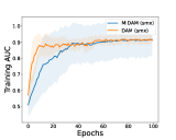
(a) smx, training, MUSK1

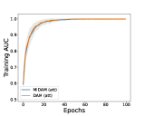
(b) att, training, MUSK1

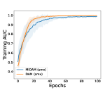
(c) smx, training, MUSK2

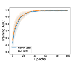
(d) att, training, MUSK2

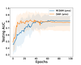
(e) smx, testing, MUSK1

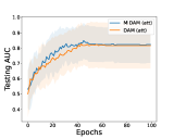
(f) att, testing, MUSK1

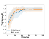
(g) smx, testing, MUSK2

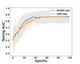
(h) att, testing, MUSK2

Figure 4: Training and testing convergence of MIDAM (XX) vs DAM (XX). The top is for training AUC, and the bottom is for testing AUC.

From the results, we observe that MIDAM (att) or MIDAM (smx) method achieves the best performance on these classical tabular benchmark datasets. This might sound surprising given that the DAM baselines use all instances for each bag for computing the pooling. To understand this, we plot the training and testing convergence curves (shown in Figure 4 in Appendix C due to limit of space). We find that the better testing peformance of our MIDAM methods is probably due to that the stochastic sampling over instances prevents overfitting (since training performance is worse) and hence improves the generalization (testing performance is better). In addition, DAM is better than CE except for DAM (att).

Table 2: The testing AUC on benchmark datasets.

Methods	MUSK1	MUSK2	Fox	Tiger	Elephant
CE (mean)	0.803(0.14)	0.805(0.113)	0.701(0.116)	0.822(0.093)	0.877(0.065)
DAM (mean)	0.832(0.147)	0.818(0.079)	0.647(0.111)	0.842(0.085)	0.897(0.053)
CE (max)	0.678(0.121)	0.84(0.106)	0.657(0.147)	0.855(0.094)	0.885(0.044)
DAM (max)	0.739(0.126)	0.859(0.09)	0.595(0.159)	0.858(0.06)	0.902(0.073)
CE (smx)	0.769(0.121)	0.851(0.111)	0.668(0.117)	0.865(0.078)	0.902(0.068)
DAM (smx)	0.806(0.118)	0.854(0.108)	0.66(0.138)	0.867(0.07)	0.902(0.052)
CE (att)	0.808(0.112)	0.76(0.122)	0.705(0.13)	0.834(0.09)	0.883(0.092)
DAM (att)	0.768(0.139)	0.757(0.154)	0.69(0.123)	0.848(0.067)	0.872(0.074)
MIDAM (smx)	0.834(0.12)	0.905(0.068)	0.622(0.188)	0.861(0.071)	0.873(0.104)
MIDAM (att)	0.826(0.107)	0.843(0.107)	0.733(0.097)	0.867(0.066)	0.906(0.069)

Table 3: The testing AUC on medical image datasets.

	Histopathological Image		MRI/OCT 3D-Image
Methods	Breast Cancer	Colon Ade.	PDGM	OCT
CE (3D)	0.925(0.061)	0.724(0.165)	0.582(0.118)	0.789(0.032)
DAM (3D)	0.725(0.2)	0.846(0.075)	0.545(0.122)	0.807(0.027)
CE (MB-mean)	0.85(0.242)	0.883(0.042)	0.616(0.023)	0.799(0.019)
DAM (MB-mean)	0.875(0.137)	0.877(0.017)	0.635(0.113)	0.839(0.029)
CE (MB-max)	0.325(0.232)	0.856(0.032)	0.462(0.108)	0.793(0.047)
DAM (MB-max)	0.475(0.215)	0.825(0.044)	0.624(0.112)	0.841(0.01)
CE (MB-smx)	0.575(0.127)	0.863(0.031)	0.491(0.111)	0.826(0.018)
DAM (MB-smx)	0.725(0.184)	0.905(0.01)	0.659(0.058)	0.829(0.008)
CE (MB-att)	0.9(0.146)	0.9(0.042)	0.564(0.072)	0.823(0.017)
DAM (MB-att)	0.875(0.112)	0.882(0.029)	0.624(0.112)	0.842(0.013)
MIDAM-smx	0.875(0.137)	0.91(0.02)	0.669(0.032)	0.848(0.01)
MIDAM-att	0.95(0.1)	0.893(0.08)	0.635(0.052)	0.843(0.012)

(a) att, Breast Cancer

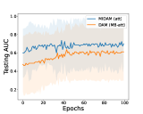
(b) att, Breast Cancer

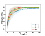
(c) MIDAM (smx), MUSK2

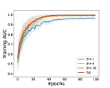
(d) MIDAM (att), MUSK2

(e) MIDAM (att), Colon Ade.

(f) MIDAM (att), Colon Ade.

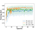
(g) MIDAM (smx), Colon Ade.

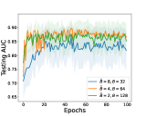
(h) MIDAM (smx), Colon Ade.

Figure 1: (a, b): Convergence of training AUC for MIDAM (att) and DAM (MB-att) on Breast Cancer data with margin $c=0.1$ and learning rate tuned in {1e-1,1e-2,1e-3}; (c, d): Convergence of training AUC with different instance-batch size by fixing bag-batch size $S_{+}=S_{-}=8$ on MUSK2 data; (e,f,g,h): Convergence of training and testing AUC with different bag-batch sizes $S_{+}=S_{-}=\frac{\hat{B}}{2}$ and instance-batch sizes ($B$) on Colon Ade. data.

(a) Positive image

(b) Prediction scores

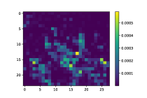
(c) Attention weights

Figure 2: Demonstration for positive example for Breast Cancer dataset. Left: original image. Middle: prediction scores for each patch. Right: attention weights for each patch.

6.2 Experiments on Medical Image datasets

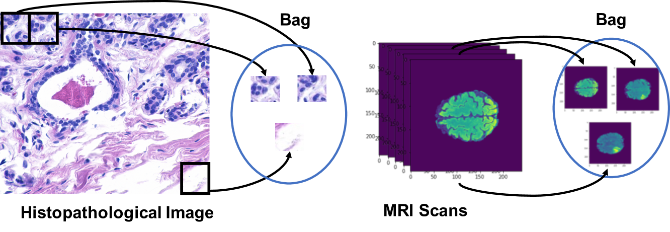
Figure 3: Illustration of MIL for medical data (Breast Cancer on the left and PDGM on the right).

We choose two histopathological image datasets, namely Breast Cancer and Colon Adenocarcinoma (Gelasca et al., 2008; Borkowski et al., 2019a). These have been used in previous deep MIL works (Ilse et al., 2018) for evaluation. Histopathological images are microscopic images of the tissue for disease examination, which are prevalent for cancer diagnosis (Borkowski et al., 2019b). Since histopathological images have a high resolution, it is difficulty to process the whole image. Hence MIL approaches are appealing that treat each image as a bag of local small batches. For Breast Cancer, there are 58 weakly labeled $896\times 768$ hematoxylin and eosin (H&E) stained whole-slide images. An image is labeled malignant if it contains breast cancer cells, otherwise it is benign (examples shown in Figure 3). We divide every image into $32\times 32$ patches. This results in 672 patches per bag. For Colon Adenocarcinoma dataset, there are originally 5000 (H&E) images for benign colon tissue and 5000 for Colon Adenocarcinoma. We uniformly randomly sample 1000 benign images and 100 Adenocarcinoma images to form the new Colon Ade. dataset for our study. We divide every $512\times 512$ image into $32\times 32$ patches and get 256 patches for each image. We also use two real-world MRI/OCT image datasets. The first data set is from the University of California San Francisco Preoperative Diffuse Glioma MRI (UCSF-PDGM) (Calabrese et al., 2022), short as PDGM in this work. The problem is to predict patients with grade II or grade IV diffuse gliomas. The second dataset contains multiple OCT images for a large number of patients (Xie et al., 2022). The goal is to predict hypertension from OCT images, which is useful for physicians to understand the relationship between eye-diseases and Hypertension. Exemplar images of two datasets are shown in Figure 3 in the Appendix C.

For all the medical images, we adopt ResNet20 as the backbone model. For AUC loss function, we apply sigmoid as normalization for the output. The weight decay is fixed as 1e-4. For all the experiments, we run 100 epochs for each trial and decrease learning rate by 10 fold at the end of the 50-th epoch and 75-th epoch. For the Breast Cancer dataset, we generate data train/test (0.9/0.1) splitting 2 times with different random seeds and conduct five-fold cross validation (10 trials). For the other datasets, we do single random train/test (0.9/0.1) splitting and conduct five-fold cross validation (5 trials). The margin parameter is tuned in {0.1,0.5,1.0} for AUC loss function. The initial learning rate is tuned in {1e-1,1e-2,1e-3} for histopathological image datasets, and is fixed as 1e-2 for PDGM, 1e-1 for OCT.

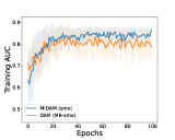
(a) smx, Breast Cancer

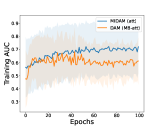
(b) att, Breast Cancer

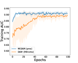
(c) smx, Colon Ade.

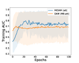
(d) att, Colon Ade.

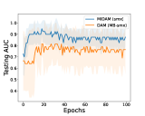
(e) smx, testing, Breast Cancer

(f) att, testing, Breast Cancer

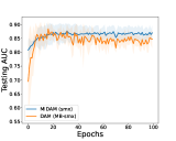
(g) smx, testing, Colon Ade.

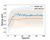
(h) att, testing, Colon Ade.

Figure 5: Training and testing convergence of MIDAM (XX) vs DAM (MB-XX). The margin $c=0.1$ and learning rate is tuned in {1e-1,1e-2,1e-3}. The top is for training AUC, and the bottom is for testing AUC.

The results are shown in Table 3. From these results, we make the following observations. (1) Our MIDAM still performs the best. Although CE (3D) on Breast Cancer, and CE (MB-att) on the two histopathological image datasets are competitive, most of the CE based approaches are less competitive with DAM based approaches. (2) By comparing MIDAM (att) with DAM (MB-att) and MIDAM (smx) with DAM (MB-smx), our methods perform consistently better. This confirms the importance of using variance-reduced stochastic pooling operations instead of the naive mini-batch based stochastic poolings. This can be also verified by comparing their training/testing convergence in Figure 1(a,b) and Figure 5 in the Appendix. (3) For Breast Cancer data, our method MIDAM (att) performs better than all baseline methods. It is notable that CE (3D) and CE (MB-att) are competitive approaches but still have worse performance than MIDAM (att). On Colon Ade. dataset, our method MIDAM (smx) performs the best and CE (MB-att) is still competitive. Finally, we see that there is no clear winner between MIDAM (att) and MIDAM (smx). (4) In general, MIL pooling based methods can achieve better performance than the traditional baseline using 3D data input. Hence, our MIDAM algorithms are a good fit for 3D medical images.

6.3 Ablation Studies

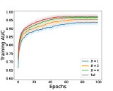
(b) MIDAM-smx, Fox

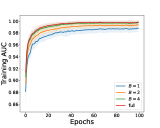
(c) MIDAM-smx, Tiger

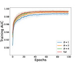
(d) MIDAM-smx, Elephant

(e) MIDAM-att, MUSK2

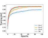
(f) MIDAM-att, Fox

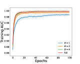
(g) MIDAM-att, Tiger

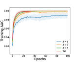
(h) MIDAM-att, Elephant

Figure 6: Training with different instance-batch sizes

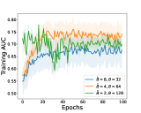
(a) smx, training, Breast Cancer

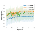
(b) att, training, Breast Cancer

(c) smx, training, Colon Ade.

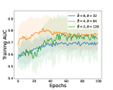
(d) att, training, Colon Ade.

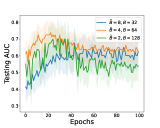
(e) smx, testing, Breast Cancer

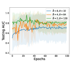
(f) att, testing, Breast Cancer

(g) smx, testing, Colon Ade.

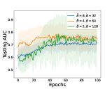
(h) att, testing, Colon Ade.

Figure 7: Ablation study for fixing the total budget per-iteration by varying bag-batch size $S_{+}=S_{-}=\hat{B}$ and instance-batch size $B$ for the proposed MIDAM approaches

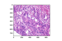
(a) Positive image

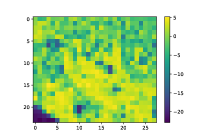
(b) Prediction scores

(c) Attention weights

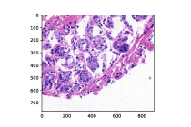
(d) Negative image

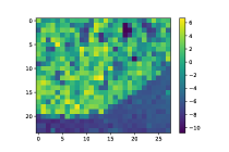
(e) Prediction scores

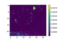
(f) Attention weights

Figure 8: Demonstrations for positive and negative examples for Breast Cancer dataset. Left: original image. Middle: prediction scores for each patch. Right: attention weights for each patch.

First, we conduct an experiment to study the influence for different instance-batch sizes ($B$) on four tabular datasets. The results on MUSK2 are shown in Figure 1 (c,d) with more plotted in Figure 6, which demonstrate our methods converge faster with a larger $B$ with fixed bag-batch size $S_{+}$ and $S_{-}$. In addition, we observe that with $B=4$ MIDAM converges to almost same level as using all instances in 100 epochs, even for the MUSK2 dataset with average bag size as 64.69. Second, we show an ablation study on the two histopathological image datasets that fixes the total budget for bag-batch-size$\times$instance-batch-size. Exemplar results are plotted in Figure 1 (e,f,g,h) with more results plotted in Figure 7. We can see that due to sampling of instances per-bag, we have more flexibility to choose the bag-batch size $S_{+}=S_{-}=\hat{B}/2$ and instance-batch size $B$ to have faster training, e.g., with $\hat{B}=4,B=64$ MIDAM converges the fastest, which demonstrates the superiority of our design. Third, we demonstrate the effectiveness of stochastic attention pooling based MIDAM on a Breast Cancer example by attention weights and prediction scores for each instance (image patch). The results are presented in Figure 2, where we can observe the lesion parts for the histopathology tissue have larger prediction scores and attention weights (the brighter patches). More demonstration on a negative examples are included in Figure 8 in Appendix C, where the attention module focus on a blank patch to generate low overall prediction score.

7 Conclusions

We have proposed efficient algorithms for multi-instance deep AUC maximization. Our algorithms are based on variance-reduced stochastic poolings in a spirit of compositional optimization to enjoy a provable convergence. We have demonstrated the effectiveness and superiority of our algorithms on benchmark datasets and real-world high-resolution medical image datasets.

8 Acknowledgement

This work is partially supported by NSF Career Award 2246753, NSF Grant 2246757 and NSF Grant 2246756.

Appendix A Technical Lemmas

Lemma 2.

Based on Assumption 1, we have that $h(\mathbf{w};\mathcal{X})$ is bounded, Lipschitz continuous, and has Lipschitz continuous gradient, i.e., there exists $B_{h},C_{h},L_{h}\geq 0$ such that $|h(\mathbf{w};\mathcal{X})|\leq B_{h}$, $\left\|\nabla h(\mathbf{w};\mathcal{X})\right\|_{2}\leq C_{h}$, and $\nabla^{2}h(\mathbf{w};\mathcal{X})\preceq L_{h}I$.

Proof.

Smoothed-max pooling: Property of the LogSumExp (LSE) function implies that

$$|h(\mathbf{w};\mathcal{X})|\leq\tau\max_{\mathbf{x}\in\mathcal{X}}\frac{|\phi_{\mathbf{w}}(\mathbf{x})|}{\tau}+(1-\tau)\log|\mathcal{X}|.$$

The norm of $\nabla h(\mathbf{w};\mathcal{X})$ can be bounded as

$$\left\|\nabla h(\mathbf{w};\mathcal{X})\right\|_{2}=\left\|\sum_{\mathbf{x}\in\mathcal{X}}\frac{\exp(\phi(\mathbf{w};\mathbf{x})/\tau)}{\sum_{\mathbf{x}\in\mathcal{X}}\exp(\phi(\mathbf{w};\mathbf{x})/\tau)}\nabla\phi(\mathbf{w};\mathbf{x})\right\|_{2}\leq C_{\phi}.$$

The norm of $\nabla^{2}h(\mathbf{w};\mathbf{x})$ can be bounded as

$$\left\|\nabla^{2}h(\mathbf{w};\mathbf{x})\right\|_{2}\leq\left\|\sum_{\mathbf{x}\in\mathcal{X}}\frac{\exp(\phi(\mathbf{w};\mathbf{x})/\tau)}{\sum_{\mathbf{x}\in\mathcal{X}}\exp(\phi(\mathbf{w};\mathbf{x})/\tau)}\left(\nabla\phi(\mathbf{w};\mathbf{x})[\nabla\phi(\mathbf{w};\mathbf{x})]^{\top}/\tau+\nabla^{2}\phi(\mathbf{w};\mathbf{x})\right)\right\|_{2}$$

$$\quad\quad+\left\|\left(\sum_{\mathbf{x}\in\mathcal{X}}\frac{\exp(\phi(\mathbf{w};\mathbf{x})/\tau)}{\sum_{x\in\mathcal{X}}\exp(\phi(\mathbf{w};\mathbf{x})/\tau)}\nabla\phi(\mathbf{w};\mathbf{x})\right)\left(\sum_{\mathbf{x}\in\mathcal{X}}\frac{\exp(\phi(\mathbf{w};\mathbf{x})/\tau)}{\sum_{x\in\mathcal{X}}\exp(\phi(\mathbf{w};\mathbf{x})/\tau)}[\nabla\phi(\mathbf{w};\mathbf{x})]^{\top}/\tau\right)\right\|_{2}\leq 2C_{\phi}^{2}/\tau+L_{\phi}.$$

Attention-based pooling: According to (3), it is clear that $|h(\mathbf{w};\mathcal{X})|\leq 1$. The norm of $\nabla h(\mathbf{w};\mathcal{X})$ can be bounded as

$$\left\|\nabla h(\mathbf{w};\mathcal{X})\right\|_{2} \leq 0.25\left\|\sum_{x\in\mathcal{X}}\frac{\exp(g(\mathbf{w};\mathbf{x}))\delta(\mathbf{w};\mathbf{x})}{\sum_{\mathbf{x}^{\prime}\in\mathcal{X}}\exp(g(\mathbf{w};\mathbf{x}^{\prime}))}\nabla g(\mathbf{w};\mathbf{x})\right\|_{2}+0.25\left\|\sum_{\mathbf{x}\in\mathcal{X}}\frac{\exp(g(\mathbf{w};\mathbf{x}))}{\sum_{\mathbf{x}^{\prime}\in\mathcal{X}}\exp(g(\mathbf{w};\mathbf{x}^{\prime}))}\nabla\delta(\mathbf{w};\mathbf{x})\right\|_{2}$$

$$\quad\quad+0.25\left|\sum_{\mathbf{x}\in\mathcal{X}}\frac{\exp(g(\mathbf{w};\mathbf{x}))\delta(\mathbf{w};\mathbf{x})}{\sum_{\mathbf{x}^{\prime}\in\mathcal{X}}\exp(g(\mathbf{w};\mathbf{x}^{\prime}))}\right|\left\|\sum_{\mathbf{x}\in\mathcal{X}}\frac{\exp(g(\mathbf{w};\mathbf{x}))}{\sum_{\mathbf{x}^{\prime}\in\mathcal{X}}\exp(g(\mathbf{w};\mathbf{x}^{\prime}))}\nabla g(\mathbf{w};\mathbf{x})\right\|_{2}\leq 0.5C_{g}B_{\delta}+0.25C_{\delta}.$$

For brevity, we denote the softmax function $s(\mathbf{w};\mathbf{x})\coloneqq\frac{\exp(g(\mathbf{w};\mathbf{x}))}{\sum_{x^{\prime}\in\mathcal{X}}\exp(g(\mathbf{w};\mathbf{x}^{\prime}))}$. The norm of $\nabla^{2}h(\mathbf{w};\mathbf{x})$ can be bounded as

$$\left\|\nabla^{2}h(\mathbf{w};\mathbf{x})\right\|_{2}$$

$$\leq 0.1\left\|\nabla h(\mathbf{w};\mathcal{X})[\nabla h(\mathbf{w};\mathcal{X})]^{\top}\right\|_{2}+0.25\left\|\sum_{\mathbf{x}\in\mathcal{X}}s(\mathbf{w};\mathbf{x})(\delta(\mathbf{w};\mathbf{x})\nabla g(\mathbf{w};\mathbf{x})+\nabla\delta(\mathbf{w};\mathbf{x}))[\nabla g(\mathbf{w};\mathbf{x})]^{\top}\right\|_{2}$$

$$+0.25\left\|\sum_{\mathbf{x}\in\mathcal{X}}s(\mathbf{w};\mathbf{x})\left(\nabla g(\mathbf{w};\mathbf{x})[\nabla\delta(\mathbf{w};\mathbf{x})]^{\top}+\delta(\mathbf{w};\mathbf{x})\nabla^{2}g(\mathbf{w};\mathbf{x})+\nabla^{2}\delta(\mathbf{w};\mathbf{x})\right)\right\|_{2}$$

$$+0.25\left\|\left(\sum_{\mathbf{x}\in\mathcal{X}}s(\mathbf{w};\mathbf{x})(\delta(\mathbf{w};\mathbf{x})\nabla g(\mathbf{w};\mathbf{x})+\nabla\delta(\mathbf{w};\mathbf{x}))\right)\left(\sum_{\mathbf{x}\in\mathcal{X}}s(\mathbf{w};\mathbf{x})(\delta(\mathbf{w};\mathbf{x})\nabla g(\mathbf{w};\mathbf{x})+\nabla\delta(\mathbf{w};\mathbf{x}))[\nabla g(\mathbf{w};\mathbf{x})]^{\top}\right)\right\|_{2}$$

$$+0.25\left\|\left(\sum_{\mathbf{x}\in\mathcal{X}}s(\mathbf{w};\mathbf{x})\nabla g(\mathbf{w};\mathbf{x})\right)\left(\sum_{\mathbf{x}\in\mathcal{X}}s(\mathbf{w};\mathbf{x})(\delta(\mathbf{w};\mathbf{x})\nabla g(\mathbf{w};\mathbf{x})+\nabla\delta(\mathbf{w};\mathbf{x}))\right)^{\top}\right\|_{2}$$

$$+0.25\left\|\left(\sum_{\mathbf{x}\in\mathcal{X}}s(\mathbf{w};\mathbf{x})\nabla g(\mathbf{w};\mathbf{x})\right)\left(\sum_{\mathbf{x}\in\mathcal{X}}s(\mathbf{w};\mathbf{x})\delta(\mathbf{w};\mathbf{x})\right)\left(\sum_{\mathbf{x}\in\mathcal{X}}s(\mathbf{w};\mathbf{x})\nabla g(\mathbf{w};\mathbf{x})\right)^{\top}\right\|_{2}$$

$$+0.25\left\|\left(\sum_{\mathbf{x}\in\mathcal{X}}s(\mathbf{w};\mathbf{x})\delta(\mathbf{w};\mathbf{x})\right)\left(\sum_{x\in\mathcal{X}}s(\mathbf{w};\mathbf{x})(\nabla g(\mathbf{w};\mathbf{x})[\nabla g(\mathbf{w};\mathbf{x})]^{\top}+\nabla^{2}g(\mathbf{w};\mathbf{x}))\right)\right\|_{2}$$

$$+0.25\left\|\left(\sum_{\mathbf{x}\in\mathcal{X}}s(\mathbf{w};\mathbf{x})\nabla g(\mathbf{w};\mathbf{x})\right)\left(\sum_{\mathbf{x}\in\mathcal{X}}s(\mathbf{w};\mathbf{x})\nabla g(\mathbf{w};\mathbf{x})\right)^{\top}\right\|_{2}$$

$$\leq 0.1C_{h}^{2}+0.5(B_{\delta}C_{g}+C_{\delta})C_{g}+0.25(C_{g}C_{\delta}+B_{\delta}L_{g}+L_{\delta})$$

$$\quad\quad+0.25(B_{\delta}C_{g}+C_{\delta})^{2}C_{g}+0.25C_{g}^{2}(B_{\delta}+1)+0.25B_{\delta}(C_{g}^{2}+L_{g}).$$

∎

Lemma 3.

Under Assumption 1, MIDAM with $\gamma\in(0,1)$, $s_{i}^{0}=0$, we have $|s_{i}^{t}|\leq B_{s}$ for all $t>0$.

Proof.

This lemma follows from Assumption 1 and the facts that $f_{1}$ is continuously differentiable on its domain and the update formula of $s_{i}$ is a convex combination. ∎

Lemma 4.

If $\eta\in(0,0.5)$ and $a^{0}=0$, $b^{0}=0$, there exist $B_{a},B_{b}>0$ $|a^{t}|\leq B_{a}$, $|b^{t}|<B_{b}$ for all $t>0$.

Proof.

Note that $G_{1,a}^{t}=-\frac{2}{|\mathcal{S}_{+}^{t}|}\sum_{i\in\mathcal{S}_{+}^{t}}(f_{2}(s_{i}^{t})-a^{t})$ and $G_{2,b}^{t}=-\frac{2}{|\mathcal{S}_{-}^{t}|}\sum_{i\in\mathcal{S}_{-}^{t}}(f_{2}(s_{i}^{t})-b^{t})$. Thus, the update formulae of $a$ and $b$ can be re-rewritten as

$$a^{t+1}=a^{t}-\eta G_{1,a}^{t}=(1-2\eta)a^{t}+2\eta\frac{1}{|\mathcal{S}_{+}^{t}|}\sum_{i\in\mathcal{S}_{+}^{t}}f_{2}(s_{i}^{t}),$$

$$b^{t+1}=b^{t}-\eta G_{2,b}^{t}=(1-2\eta)b^{t}+2\eta\frac{1}{|\mathcal{S}_{-}^{t}|}\sum_{i\in\mathcal{S}_{-}^{t}}f_{2}(s_{i}^{t}).$$

Due to Lemma 3 and the fact that $f_{2}$ is continuously differentiable on its domain, $a^{t}$ and $b^{t}$ are bounded in all iterations as long as $\eta\in(0,0.5)$ such that the update formulae of $a^{t}$ and $b^{t}$ are convex combinations. ∎

Lemma 5.

Under Assumption 1, there exists $L_{F}>0$ such that $\nabla F$ is $L_{F}$-Lipschitz continuous.

Proof.

Note that $h(\mathbf{w};\mathcal{X}_{i})=f_{2}(f_{1}(\mathbf{w};\mathcal{X}_{i}))$, $\nabla h(\mathbf{w};\mathcal{X}_{i})=\nabla f_{1}(\mathbf{w};\mathcal{X}_{i})\nabla f_{2}(f_{1}(\mathbf{w};\mathcal{X}_{i}))$. For distinct $(\mathbf{w},a,b,\alpha)$ and $(\mathbf{w}^{\prime},a^{\prime},b^{\prime},\alpha^{\prime})$, we have

$$\left\|\nabla_{(\mathbf{w},a,b)}F(\mathbf{w},a,b,\alpha)-\nabla_{(\mathbf{w},a,b)}F(\mathbf{w}^{\prime},a^{\prime},b^{\prime},\alpha^{\prime})\right\|_{2}+|\nabla_{\alpha}F(\mathbf{w},a,b,\alpha)-\nabla_{\alpha}F(\mathbf{w}^{\prime},a^{\prime},b^{\prime},\alpha^{\prime})|$$

$$\leq\left\|\frac{2}{|\mathcal{D}_{+}|}\sum_{i\in\mathcal{D}_{+}}\left(\nabla h(\mathbf{w};\mathcal{X}_{i})(h(\mathbf{w};\mathcal{X}_{i})-a)-\nabla h(\mathbf{w}^{\prime};\mathcal{X}_{i})(h(\mathbf{w}^{\prime};\mathcal{X}_{i})-a^{\prime})\right)\right\|_{2}$$

$$+\left\|\frac{2}{|\mathcal{D}_{-}|}\sum_{i\in\mathcal{D}_{-}}\left(\nabla h(\mathbf{w};\mathcal{X}_{i})(h(\mathbf{w};\mathcal{X}_{i})-b)-\nabla h(\mathbf{w}^{\prime};\mathcal{X}_{i})(h(\mathbf{w}^{\prime};\mathcal{X}_{i})-b^{\prime})\right)\right\|_{2}$$

$$+\left\|\alpha\frac{1}{|\mathcal{D}_{-}|}\sum_{i\in\mathcal{D}_{-}}\nabla h(\mathbf{w};\mathcal{X}_{i})-\alpha^{\prime}\frac{1}{|\mathcal{D}_{-}|}\sum_{i\in\mathcal{D}_{-}}\nabla h(\mathbf{w}^{\prime};\mathcal{X}_{i})\right\|_{2}+\left\|\alpha\frac{1}{|\mathcal{D}_{+}|}\sum_{i\in\mathcal{D}_{+}}\nabla h(\mathbf{w};\mathcal{X}_{i})-\alpha^{\prime}\frac{1}{|\mathcal{D}_{+}|}\sum_{i\in\mathcal{D}_{+}}\nabla h(\mathbf{w}^{\prime};\mathcal{X}_{i})\right\|_{2}$$

$$+\left\|\frac{2}{|\mathcal{D}_{+}|}\sum_{i\in\mathcal{D}_{+}}(h(\mathbf{w};\mathcal{X}_{i})-a)-\frac{2}{|\mathcal{D}_{+}|}\sum_{i\in\mathcal{D}_{+}}(h(\mathbf{w}^{\prime};\mathcal{X}_{i})-a^{\prime})\right\|_{2}$$

$$+\left\|\frac{2}{|\mathcal{D}_{+}|}\sum_{i\in\mathcal{D}_{+}}(h(\mathbf{w};\mathcal{X}_{i})-b)-\frac{2}{|\mathcal{D}_{+}|}\sum_{i\in\mathcal{D}_{+}}(h(\mathbf{w}^{\prime};\mathcal{X}_{i})-b^{\prime})\right\|_{2}$$

$$+|\alpha-\alpha^{\prime}|+\left\|\frac{1}{|\mathcal{D}_{-}|}\sum_{i\in\mathcal{D}_{-}}h(\mathbf{w};\mathcal{X}_{i})-\frac{1}{|\mathcal{D}_{-}|}\sum_{i\in\mathcal{D}_{-}}h(\mathbf{w}^{\prime};\mathcal{X}_{i})\right\|_{2}+\left\|\frac{1}{|\mathcal{D}_{+}|}\sum_{i\in\mathcal{D}_{+}}h(\mathbf{w};\mathcal{X}_{i})-\frac{1}{|\mathcal{D}_{+}|}\sum_{i\in\mathcal{D}_{+}}h(\mathbf{w}^{\prime};\mathcal{X}_{i})\right\|_{2}$$

$$\leq 2(2L_{h}B_{h}+2C_{h}^{2}+(B_{a}+B_{b})L_{h}+B_{\Omega}L_{h}+3C_{h})\left\|\mathbf{w}-\mathbf{w}^{\prime}\right\|_{2}$$

$$\quad\quad+2(C_{h}+1)|a-a^{\prime}|+2(C_{h}+1)|b-b^{\prime}|+2(C_{h}+1)|\alpha-\alpha^{\prime}|.$$

∎

Lemma 6 (Lemma 4.3 in Lin et al. (2019)).

For an $F$ defined in (4) that has Lipschitz continuous gradient and $\Phi(\mathbf{w},a,b)\coloneqq\max_{\alpha\in\Omega}F(\mathbf{w},a,b,\alpha)$ with a convex and bounded $\Omega$, we have that $\Phi(\mathbf{w},a,b)$ is $L_{\Phi}$-smooth and $\nabla\Phi(\mathbf{w},a,b)=\nabla_{(\mathbf{w},a,b)}F(\mathbf{w},a,b,\alpha^{*}(\mathbf{w},a,b))$. Besides, $\alpha^{*}(\mathbf{w},a,b)$ is $1$-Lipschitz continuous.

We define $\mathbf{v}\coloneqq\begin{bmatrix}\mathbf{v}_{1}\\ \mathbf{v}_{2}\\ \mathbf{v}_{3}\end{bmatrix}$, $W\coloneqq\begin{bmatrix}\mathbf{w}\\ a\\ b\end{bmatrix}$, and $G_{W}^{t}=\begin{bmatrix}G_{1,\mathbf{w}}^{t}+G_{2,\mathbf{w}}^{t}+G_{3,\mathbf{w}}^{t}\\ G_{1,a}^{t}\\ G_{2,b}^{t}\end{bmatrix}$, $\bar{G}_{W}^{t}=\begin{bmatrix}\bar{G}_{1,\mathbf{w}}^{t}+\bar{G}_{2,\mathbf{w}}^{t}+\bar{G}_{3,\mathbf{w}}^{t}\\ \bar{G}_{1,a}^{t}\\ \bar{G}_{2,b}^{t}\end{bmatrix}$, where

$$\bar{G}^{t}_{1,\mathbf{w}}=\hat{\mathbb{E}}_{i\in\mathcal{S}_{+}^{t}}\nabla f_{1}(\mathbf{w}^{t};\mathcal{B}_{i}^{t})\nabla f_{2}(f_{1}(\mathbf{w}^{t};\mathcal{X}_{i}))\nabla_{1}f(f_{2}(f_{1}(\mathbf{w}^{t};\mathcal{X}_{i})),a^{t}),$$

$$\bar{G}^{t}_{2,\mathbf{w}}=\hat{\mathbb{E}}_{i\in\mathcal{S}_{-}^{t}}\nabla f_{1}(\mathbf{w}^{t};\mathcal{B}_{i}^{t})\nabla f_{2}(f_{1}(\mathbf{w}^{t};\mathcal{X}_{i}))\nabla_{1}f(f_{2}(f_{1}(\mathbf{w}^{t};\mathcal{X}_{i})),b^{t}),$$

$$\bar{G}^{t}_{3,\mathbf{w}}=\alpha^{t}\cdot\left(\hat{\mathbb{E}}_{i\in\mathcal{S}_{-}^{t}}\nabla f_{1}(\mathbf{w}^{t};\mathcal{B}_{i}^{t})\nabla f_{2}(f_{1}(\mathbf{w}^{t};\mathcal{X}_{i}))-\hat{\mathbb{E}}_{i\in\mathcal{S}_{+}^{t}}\nabla f_{1}(\mathbf{w}^{t};\mathcal{B}_{i}^{t})\nabla f_{2}(f_{1}(\mathbf{w}^{t};\mathcal{X}_{i}))\right),$$

$$\bar{G}^{t}_{1,a}=\hat{\mathbb{E}}_{i\in\mathcal{S}_{+}^{t}}\nabla_{2}f(f_{2}(f_{1}(\mathbf{w}^{t};\mathcal{X}_{i})),a^{t}),$$

$$\bar{G}^{t}_{2,b}=\hat{\mathbb{E}}_{i\in\mathcal{S}_{-}^{t}}\nabla_{2}f(f_{2}(f_{1}(\mathbf{w}^{t};\mathcal{X}_{i})),b^{t}).$$

Lemma 7 (Lemma 11 in Wang et al. (2021a)).

Suppose that $X=\frac{1}{n}\sum_{i=1}^{n}X_{i}$. If we sample a size-$B$ minibatch $\mathcal{B}$ from $\{1,\ldots,n\}$ uniformly at random, we have $\mathbb{E}\left[\frac{1}{B}\sum_{i\in\mathcal{B}}(X_{i}-X)\right]=0$ and

$$\mathbb{E}\left[\left\|\frac{1}{B}\sum_{i\in\mathcal{B}}(X_{i}-X)\right\|^{2}\right]\leq\frac{n-B}{B(n-1)}\frac{1}{n}\sum_{i=1}^{n}\left\|X_{i}-X\right\|^{2}\leq\frac{n-B}{B(n-1)}\frac{1}{n}\sum_{i=1}^{n}\left\|X_{i}\right\|^{2}.$$

Lemma 8.

Under Assumption 1, there exists $C_{G},C_{\Upsilon}>0$ for MIDAM such that

$$\sum_{t=0}^{T-1}\mathbb{E}\left[\Delta^{t}\right] \leq\frac{\Delta^{0}}{\beta_{1}}+2T\beta_{1}C_{G}+5L_{F}^{2}\sum_{t=0}^{T-1}\mathbb{E}\left[\Psi^{t+1}\right]+\frac{3\eta^{2}L_{\Phi}^{2}}{\beta_{1}^{2}}\sum_{t=0}^{T-1}\mathbb{E}\left[\left\|\mathbf{v}^{t}\right\|_{2}^{2}\right]+5C_{\Upsilon}\sum_{t=0}^{T-1}\mathbb{E}\left[\Upsilon_{+}^{t+1}\right]+5C_{\Upsilon}\sum_{t=0}^{T-1}\mathbb{E}\left[\Upsilon_{-}^{t+1}\right]$$

$$\quad\quad+5C_{\Upsilon}\sum_{t=0}^{T-1}\frac{1}{D_{+}}\mathbb{E}\left[\sum_{i\in\mathcal{S}_{+}^{t}}\left\|s_{i}^{t+1}-s_{i}^{t}\right\|_{2}^{2}\right]+5C_{\Upsilon}\sum_{t=0}^{T-1}\frac{1}{D_{-}}\mathbb{E}\left[\sum_{i\in\mathcal{S}_{-}^{t}}\left\|s_{i}^{t+1}-s_{i}^{t}\right\|_{2}^{2}\right].$$

where $\Delta^{t}\coloneqq\left\|\mathbf{v}^{t}-\nabla\Phi(W^{t})\right\|_{2}^{2}$, $\Upsilon_{+}^{t}\coloneqq\frac{1}{D_{+}}\sum_{i\in\mathcal{D}_{+}}\left\|s_{i}^{t}-f_{1}(\mathbf{w}^{t};\mathcal{X}_{i})\right\|_{2}^{2}$, $\Upsilon_{-}^{t}\coloneqq\frac{1}{D_{-}}\sum_{i\in\mathcal{D}_{+}}\left\|s_{i}^{t}-f_{1}(\mathbf{w}^{t};\mathcal{X}_{i})\right\|_{2}^{2}$, $\Psi^{t}\coloneqq\left\|\alpha^{t}-\alpha^{*}(W^{t})\right\|_{2}^{2}$.

Proof.

Based on the update rule of $\mathbf{v}^{t}$, we have

$$\mathbb{E}_{t+1}\left[\Delta^{t+1}\right]=\mathbb{E}_{t}\left[\left\|\mathbf{v}^{t+1}-\nabla\Phi(W^{t+1})\right\|_{2}^{2}\right]=\mathbb{E}_{t}\left[\left\|\mathbf{v}^{t+1}-\nabla_{W}F(W^{t+1},\alpha^{*}(W^{t+1}))\right\|_{2}^{2}\right]$$

$$=\mathbb{E}_{t+1}\left[\left\|(1-\beta_{1})\mathbf{v}^{t}+\beta_{1}G_{W}^{t+1}-\nabla_{W}F(W^{t+1},\alpha^{*}(W^{t+1}))\right\|_{2}^{2}\right]$$

$$=\mathbb{E}_{t+1}\left[\left\|(1-\beta_{1})\underbrace{(\mathbf{v}^{t}-\nabla\Phi(W^{t}))}_{\clubsuit}+(1-\beta_{1})\underbrace{(\nabla\Phi(W^{t})-\nabla\Phi(W^{t+1}))}_{\heartsuit}+\beta_{1}(G_{W}^{t+1}-\bar{G}_{W}^{t+1})\right.\right.$$

$$\quad\quad\quad\quad\left.\left.+\beta_{1}\underbrace{(\bar{G}_{W}^{t+1}-\nabla_{W}F(W^{t+1},\alpha^{t+1}))}_{\diamondsuit}+\beta_{1}\underbrace{(\nabla_{W}F(W^{t+1},\alpha^{t+1})-\nabla\Phi(W^{t+1}))}_{\spadesuit}\right\|_{2}^{2}\right].$$

Note that $\mathbb{E}_{t+1}[\clubsuit\cdot\diamondsuit]=0$, $\mathbb{E}_{t+1}[\heartsuit\cdot\diamondsuit]=0$, $\mathbb{E}_{t+1}[\spadesuit\cdot\diamondsuit]=0$. Then,

$$\mathbb{E}_{t+1}\left[\Delta^{t+1}\right]$$

$$=(1-\beta_{1})^{2}\Delta^{t}+(1-\beta_{1})^{2}\left\|\nabla\Phi(W^{t})-\nabla\Phi(W^{t+1})\right\|_{2}^{2}+\beta_{1}^{2}\mathbb{E}_{t+1}[\left\|G_{W}^{t+1}-\bar{G}_{W}^{t+1}\right\|_{2}^{2}]$$

$$\quad\quad+\beta_{1}^{2}\mathbb{E}_{t+1}[\left\|\bar{G}_{W}^{t+1}-\nabla_{W}F(W^{t+1},\alpha^{t+1})\right\|_{2}^{2}]+\beta_{1}^{2}\left\|\nabla_{W}F(W^{t+1},\alpha^{t+1})-\nabla\Phi(W^{t+1})\right\|_{2}^{2}$$

$$\quad\quad+2(1-\beta_{1})^{2}\left\langle\mathbf{v}^{t}-\nabla\Phi(W^{t}),\,\nabla\Phi(W^{t})-\nabla\Phi(W^{t+1})\right\rangle+2\beta_{1}(1-\beta_{1})\mathbb{E}_{t+1}[\left\langle\mathbf{v}^{t}-\nabla\Phi(W^{t}),\,G_{W}^{t+1}-\bar{G}_{W}^{t+1}\right\rangle]$$

$$\quad\quad+2\beta_{1}(1-\beta_{1})\mathbb{E}_{t+1}[\left\langle\mathbf{v}^{t}-\nabla\Phi(W^{t}),\,\nabla_{W}F(W^{t+1},\alpha^{t+1})-\nabla\Phi(W^{t+1})\right\rangle]$$

$$\quad\quad+2\beta_{1}(1-\beta_{1})\mathbb{E}_{t+1}[\left\langle\nabla\Phi(W^{t})-\nabla\Phi(W^{t+1}),\,G_{W}^{t+1}-\bar{G}_{W}^{t+1}\right\rangle]$$

$$\quad\quad+2\beta_{1}(1-\beta_{1})\mathbb{E}_{t+1}[\left\langle\nabla\Phi(W^{t})-\nabla\Phi(W^{t+1}),\,\nabla_{W}F(W^{t+1},\alpha^{t+1})-\nabla\Phi(W^{t+1})\right\rangle]$$

$$\quad\quad+2\beta_{1}^{2}\mathbb{E}_{t+1}[\left\langle G_{W}^{t+1}-\bar{G}_{W}^{t+1},\,\bar{G}_{W}^{t+1}-\nabla_{W}F(W^{t+1},\alpha^{t+1})\right\rangle]$$

$$\quad\quad+2\beta_{1}^{2}\mathbb{E}_{t+1}[\left\langle G_{W}^{t+1}-\bar{G}_{W}^{t+1},\,\nabla_{W}F(W^{t+1},\alpha^{t+1})-\nabla\Phi(W^{t+1})\right\rangle].$$

Use Young’s inequality for products.

$$\mathbb{E}_{t+1}\left[\Delta^{t+1}\right]$$

$$\leq(1-\beta_{1})^{2}(1+\beta_{1})\Delta^{t}+\frac{3(1-\beta_{1})^{2}(1+\beta_{1})}{\beta_{1}}\left\|\nabla\Phi(W^{t})-\nabla\Phi(W^{t+1})\right\|_{2}^{2}+2\beta_{1}^{2}\mathbb{E}_{t+1}[\left\|\bar{G}_{W}^{t+1}-\nabla_{W}F(W^{t+1},\alpha^{t+1})\right\|_{2}^{2}]$$

$$\quad\quad+(3\beta_{1}+5\beta_{1}^{2}/3)\left\|G_{W}^{t+1}-\bar{G}_{W}^{t+1}\right\|_{2}^{2}+(3\beta_{1}+5\beta_{1}^{2}/3)\mathbb{E}_{t+1}[\left\|\nabla_{W}F(W^{t+1},\alpha^{t+1})-\nabla\Phi(W^{t+1})\right\|_{2}^{2}]$$

$$\leq(1-\beta_{1})\Delta^{t}+\frac{3L_{\Phi}^{2}\eta^{2}}{\beta_{1}}\left\|\mathbf{v}^{t}\right\|_{2}^{2}+2\beta_{1}^{2}\mathbb{E}_{t+1}[\left\|\bar{G}_{W}^{t+1}-\nabla_{W}F(W^{t+1},\alpha^{t+1})\right\|_{2}^{2}]$$

$$\quad\quad+5\beta_{1}\underbrace{\mathbb{E}_{t+1}[\left\|G_{W}^{t+1}-\bar{G}_{W}^{t+1}\right\|_{2}^{2}]}_{\triangle}+5\beta_{1}\left\|\nabla_{W}F(W^{t+1},\alpha^{t+1})-\nabla\Phi(W^{t+1})\right\|_{2}^{2}.$$

Note that $s_{i}^{t}$, $a^{t}$, $b^{t}$, $\alpha^{t}$ are bounded due to Lemma 3, Lemma 4 and the projection step of updating $\alpha$. Besides, there exist $B_{f_{1}},C_{f_{1}},B_{f_{2}},C_{f_{2}},L_{f_{2}}>0$ such that $\left\|f_{1}\right\|_{2}\leq B_{f_{1}},\left\|\nabla f_{1}\right\|_{2}\leq C_{f_{1}}$, $\left\|f_{2}\right\|_{2}\leq B_{f_{2}},\left\|\nabla f_{2}\right\|_{2}\leq C_{f_{2}},\left\|\nabla^{2}f_{2}\right\|_{2}\leq L_{f_{2}}$ due to Assumption 1. Then, the definition of $\bar{G}_{1,\mathbf{w}}^{t+1}$, $\bar{G}_{2,\mathbf{w}}^{t+1}$, $\bar{G}_{3,\mathbf{w}}^{t+1}$, $\bar{G}_{1,a}^{t+1}$, $\bar{G}_{2,b}^{t+1}$ leads to

$$\mathbb{E}_{t+1}[\left\|\bar{G}_{W}^{t+1}-\nabla_{W}F(W^{t+1},\alpha^{t+1})\right\|_{2}^{2}]$$

$$=\mathbb{E}_{t+1}[\left\|\bar{G}_{1,\mathbf{w}}^{t+1}+\bar{G}_{2,\mathbf{w}}^{t+1}+\bar{G}_{3,\mathbf{w}}^{t+1}-\nabla_{\mathbf{w}}F_{1}(\mathbf{w}^{t+1},a^{t+1})-\nabla_{\mathbf{w}}F_{2}(\mathbf{w}^{t+1},b^{t+1})-\nabla_{\mathbf{w}}F_{3}(\mathbf{w}^{t+1},\alpha^{t+1})\right\|_{2}^{2}]$$

$$\quad\quad+\mathbb{E}_{t+1}[\left\|\bar{G}_{1,a}^{t+1}-\nabla_{a}F_{1}(\mathbf{w}^{t+1},a^{t+1})\right\|_{2}^{2}]+\mathbb{E}_{t+1}[\left\|\bar{G}_{2,b}^{t+1}-\nabla_{a}F_{2}(\mathbf{w}^{t+1},b^{t+1})\right\|_{2}^{2}]$$

$$\leq 3\mathbb{E}_{t+1}[\left\|\bar{G}_{1,\mathbf{w}}^{t+1}-\nabla_{\mathbf{w}}F_{1}(\mathbf{w}^{t+1},a^{t+1})\right\|_{2}^{2}]+3\mathbb{E}_{t+1}[\left\|\bar{G}_{2,\mathbf{w}}^{t+1}-\nabla_{\mathbf{w}}F_{2}(\mathbf{w}^{t+1},b^{t+1})\right\|_{2}^{2}]$$

$$\quad\quad+3\mathbb{E}_{t+1}[\left\|\bar{G}_{3,\mathbf{w}}^{t+1}-\nabla_{\mathbf{w}}F_{3}(\mathbf{w}^{t+1},\alpha^{t+1})\right\|_{2}^{2}]$$

$$\quad\quad+\mathbb{E}_{t+1}[\left\|\bar{G}_{1,a}^{t+1}-\nabla_{a}F_{1}(\mathbf{w}^{t+1},a^{t+1})\right\|_{2}^{2}]+\mathbb{E}_{t+1}[\left\|\bar{G}_{2,b}^{t+1}-\nabla_{a}F_{2}(\mathbf{w}^{t+1},b^{t+1})\right\|_{2}^{2}]$$

$$\leq 12C_{f_{1}}^{2}C_{f_{2}}^{2}(2B_{f_{2}}^{2}+B_{a}^{2}+B_{b}^{2})+6B_{\Omega}^{2}C_{f_{1}}^{2}C_{f_{2}}^{2}+4(2B_{f_{2}}^{2}+B_{a}^{2}+B_{b}^{2}).$$

We define $C_{G}\coloneqq 12C_{f_{1}}^{2}C_{f_{2}}^{2}(2B_{f_{2}}^{2}+B_{a}^{2}+B_{b}^{2})+6B_{\Omega}^{2}C_{f_{1}}^{2}C_{f_{2}}^{2}+4(2B_{f_{2}}^{2}+B_{a}^{2}+B_{b}^{2})$. Besides,

$$\left\|\nabla_{W}F(W^{t+1},\alpha^{t+1})-\nabla\Phi(W^{t+1})\right\|_{2}^{2} =\left\|\nabla_{W}F(W^{t+1},\alpha^{t+1})-\nabla_{W}F(W^{t+1},\alpha^{*}(W^{t+1}))\right\|_{2}^{2}$$

$$\leq L_{F}^{2}\left\|\alpha^{t+1}-\alpha^{*}(W^{t+1})\right\|_{2}^{2}.$$

Next, we turn to bound the $\triangle$ term.

$$\mathbb{E}_{t+1}[\left\|G_{W}^{t+1}-\bar{G}_{W}^{t+1}\right\|_{2}^{2}]$$

$$\leq 3\mathbb{E}_{t+1}\left[\left\|\frac{2}{|\mathcal{S}_{+}^{t+1}|}\sum_{i\in\mathcal{S}_{+}^{t+1}}\nabla f_{1}(\mathbf{w}^{t+1};\mathcal{B}_{i}^{t+1})\left(\nabla f_{2}(s_{i}^{t})f_{2}(s_{i}^{t})-\nabla f_{2}(f_{1}(\mathbf{w}^{t+1};\mathcal{X}_{i}))f_{2}(f_{1}(\mathbf{w}^{t+1};\mathcal{X}_{i}))\right)\right\|_{2}^{2}\right]$$

$$\quad\quad+3\mathbb{E}_{t+1}\left[\left\|\frac{2}{|\mathcal{S}_{-}^{t+1}|}\sum_{i\in\mathcal{S}_{-}^{t+1}}\nabla f_{1}(\mathbf{w}^{t+1};\mathcal{B}_{i}^{t+1})\left(\nabla f_{2}(s_{i}^{t})f_{2}(s_{i}^{t})-\nabla f_{2}(f_{1}(\mathbf{w}^{t+1};\mathcal{X}_{i}))f_{2}(f_{1}(\mathbf{w}^{t+1};\mathcal{X}_{i}))\right)\right\|_{2}^{2}\right]$$

$$\quad\quad+6\mathbb{E}_{t+1}\left[\left\|\alpha^{t+1}\left(\frac{1}{|\mathcal{S}_{-}^{t+1}|}\sum_{i\in\mathcal{S}_{-}^{t+1}}\nabla f_{1}(\mathbf{w}^{t};\mathcal{B}_{i}^{t})\left(\nabla f_{2}(s_{i}^{t})-\nabla f_{2}(f_{1}(\mathbf{w}^{t+1};\mathcal{X}_{i}))\right)\right)\right\|_{2}^{2}\right]$$

$$\quad\quad+6\mathbb{E}_{t+1}\left[\left\|\alpha^{t+1}\left(\frac{1}{|\mathcal{S}_{+}^{t+1}|}\sum_{i\in\mathcal{S}_{+}^{t+1}}\nabla f_{1}(\mathbf{w}^{t};\mathcal{B}_{i}^{t})\left(\nabla f_{2}(s_{i}^{t})-\nabla f_{2}(f_{1}(\mathbf{w}^{t+1};\mathcal{X}_{i}))\right)\right)\right\|_{2}^{2}\right]$$

$$\quad\quad+\mathbb{E}_{t+1}\left[\left\|\frac{2}{|\mathcal{S}_{+}^{t+1}|}\sum_{i\in\mathcal{S}_{+}^{t+1}}(f_{2}(s_{i}^{t})-f_{2}(f_{1}(\mathbf{w}^{t+1};\mathcal{X}_{i})))\right\|_{2}^{2}\right]+\mathbb{E}_{t+1}\left[\left\|\frac{2}{|\mathcal{S}_{-}^{t+1}|}\sum_{i\in\mathcal{S}_{-}^{t+1}}(f_{2}(s_{i}^{t})-f_{2}(f_{1}(\mathbf{w}^{t+1};\mathcal{X}_{i})))\right\|_{2}^{2}\right].$$

Note that $s_{i}^{t}$ and $\mathbf{w}^{t+1}$ are independent of $\mathcal{S}_{+}^{t+1}$ and $\mathcal{S}_{-}^{t+1}$.

$$\mathbb{E}_{t+1}[\left\|G_{W}^{t+1}-\bar{G}_{W}^{t+1}\right\|_{2}^{2}]$$

$$\leq 12C_{f_{1}}^{2}\frac{1}{D_{+}}\sum_{i\in\mathcal{D}_{+}}\left\|\nabla f_{2}(s_{i}^{t})f_{2}(s_{i}^{t})-\nabla f_{2}(f_{1}(\mathbf{w}^{t+1};\mathcal{X}_{i}))f_{2}(f_{1}(\mathbf{w}^{t+1};\mathcal{X}_{i}))\right\|_{2}^{2}$$

$$\quad\quad+12C_{f_{1}}^{2}\frac{1}{D_{-}}\sum_{i\in\mathcal{D}_{-}}\left\|\nabla f_{2}(s_{i}^{t})f_{2}(s_{i}^{t})-\nabla f_{2}(f_{1}(\mathbf{w}^{t+1};\mathcal{X}_{i}))f_{2}(f_{1}(\mathbf{w}^{t+1};\mathcal{X}_{i}))\right\|_{2}^{2}$$

$$\quad\quad+6B_{\Omega}^{2}C_{f_{1}}^{2}L_{f_{2}}^{2}\frac{1}{D_{+}}\sum_{i\in\mathcal{D}_{+}}\left\|s_{i}^{t}-f_{1}(\mathbf{w}^{t+1};\mathcal{X}_{i})\right\|_{2}^{2}+6B_{\Omega}^{2}C_{f_{1}}^{2}L_{f_{2}}^{2}\frac{1}{D_{-}}\sum_{i\in\mathcal{D}_{-}}\left\|s_{i}^{t}-f_{1}(\mathbf{w}^{t+1};\mathcal{X}_{i})\right\|_{2}^{2}$$

$$\quad\quad+4C_{f_{2}}^{2}\frac{1}{D_{+}}\sum_{i\in\mathcal{D}_{+}}\left\|s_{i}^{t}-f_{1}(\mathbf{w}^{t+1};\mathcal{X}_{i})\right\|_{2}^{2}+4C_{f_{2}}^{2}\frac{1}{D_{-}}\sum_{i\in\mathcal{D}_{-}}\left\|s_{i}^{t}-f_{1}(\mathbf{w}^{t+1};\mathcal{X}_{i})\right\|_{2}^{2}$$

$$\leq C_{\Upsilon}\left(\frac{1}{D_{+}}\mathbb{E}_{t+1}\left[\sum_{i\in\mathcal{D}_{+}}\left\|s_{i}^{t+1}-f_{1}(\mathbf{w}^{t+1};\mathcal{X}_{i})\right\|_{2}^{2}\right]+\frac{1}{D_{-}}\mathbb{E}_{t+1}\left[\sum_{i\in\mathcal{D}_{-}}\left\|s_{i}^{t+1}-f_{1}(\mathbf{w}^{t+1};\mathcal{X}_{i})\right\|_{2}^{2}\right]\right)$$

$$\quad\quad+C_{\Upsilon}\left(\frac{1}{D_{+}}\mathbb{E}_{t+1}\left[\sum_{i\in\mathcal{D}_{+}}\left\|s_{i}^{t+1}-s_{i}^{t}\right\|_{2}^{2}\right]+\frac{1}{D_{-}}\mathbb{E}_{t+1}\left[\sum_{i\in\mathcal{D}_{-}}\left\|s_{i}^{t+1}-s_{i}^{t}\right\|_{2}^{2}\right]\right),$$

where we define $C_{\Upsilon}\coloneqq 48C_{f_{1}}^{2}(C_{f_{2}}^{4}+B_{f_{2}}^{2}L_{f_{2}}^{2})+12C_{f_{1}}^{2}B_{\Omega}^{2}L_{f_{2}}^{2}+8C_{f_{2}}^{2}$. Note that $s_{i}^{t+1}=s_{i}^{t}$ for those $i\not\in\mathcal{S}_{+}^{t}\cup\mathcal{S}_{-}^{t}$. Then,

$$\sum_{i\in\mathcal{D}_{+}}\left\|s_{i}^{t+1}-s_{i}^{t}\right\|_{2}^{2}=\sum_{i\in\mathcal{S}_{+}^{t}}\left\|s_{i}^{t+1}-s_{i}^{t}\right\|_{2}^{2},\quad\sum_{i\in\mathcal{D}_{-}}\left\|s_{i}^{t+1}-s_{i}^{t}\right\|_{2}^{2}=\sum_{i\in\mathcal{S}_{-}^{t}}\left\|s_{i}^{t+1}-s_{i}^{t}\right\|_{2}^{2}$$

We define

$$\Upsilon_{+}^{t}\coloneqq\frac{1}{D_{+}}\sum_{i\in\mathcal{D}_{+}}\left\|s_{i}^{t}-f_{1}(\mathbf{w}^{t};\mathcal{X}_{i})\right\|_{2}^{2},\quad\Upsilon_{-}^{t}\coloneqq\frac{1}{D_{-}}\sum_{i\in\mathcal{D}_{+}}\left\|s_{i}^{t}-f_{1}(\mathbf{w}^{t};\mathcal{X}_{i})\right\|_{2}^{2},\quad\Psi^{t}=\left\|\alpha^{t}-\alpha^{*}(W^{t})\right\|_{2}^{2},$$

such that

$$\mathbb{E}_{t+1}[\Delta^{t+1}] \leq(1-\beta_{1})\Delta^{t}+\frac{3L_{\Phi}^{2}\eta^{2}}{\beta_{1}}\left\|\mathbf{v}^{t}\right\|_{2}^{2}+2\beta_{1}^{2}C_{G}+5\beta_{1}C_{\Upsilon}\left(\mathbb{E}_{t+1}[\Upsilon_{+}^{t+1}]+\mathbb{E}_{t+1}[\Upsilon_{-}^{t+1}]\right)+5\beta_{1}L_{F}^{2}\Psi^{t+1}$$

$$\quad\quad+5\beta_{1}C_{\Upsilon}\left(\frac{1}{D_{+}}\mathbb{E}_{t+1}\left[\sum_{i\in\mathcal{S}_{+}^{t}}\left\|s_{i}^{t+1}-s_{i}^{t}\right\|_{2}^{2}\right]+\frac{1}{D_{-}}\mathbb{E}_{t+1}\left[\sum_{i\in\mathcal{S}_{-}^{t}}\left\|s_{i}^{t+1}-s_{i}^{t}\right\|_{2}^{2}\right]\right).$$

Sum over $t=0,\dotsc,T-1$.

$$\sum_{t=0}^{T-1}\mathbb{E}\left[\Delta^{t}\right] \leq\frac{\Delta^{0}}{\beta_{1}}+2T\beta_{1}C_{G}+5L_{F}^{2}\sum_{t=0}^{T-1}\mathbb{E}\left[\Psi^{t+1}\right]+\frac{3\eta^{2}L_{\Phi}^{2}}{\beta_{1}^{2}}\sum_{t=0}^{T-1}\mathbb{E}\left[\left\|\mathbf{v}^{t}\right\|_{2}^{2}\right]+5C_{\Upsilon}\sum_{t=0}^{T-1}\mathbb{E}\left[\Upsilon_{+}^{t+1}\right]+5C_{\Upsilon}\sum_{t=0}^{T-1}\mathbb{E}\left[\Upsilon_{-}^{t+1}\right]$$

$$\quad\quad+5C_{\Upsilon}\sum_{t=0}^{T-1}\frac{1}{D_{+}}\mathbb{E}\left[\sum_{i\in\mathcal{S}_{+}^{t}}\left\|s_{i}^{t+1}-s_{i}^{t}\right\|_{2}^{2}\right]+5C_{\Upsilon}\sum_{t=0}^{T-1}\frac{1}{D_{-}}\mathbb{E}\left[\sum_{i\in\mathcal{S}_{-}^{t}}\left\|s_{i}^{t+1}-s_{i}^{t}\right\|_{2}^{2}\right].$$

∎

Lemma 9 (Lemma 1 in Wang & Yang (2022)).

Suppose that $|\mathcal{S}_{+}^{t}|\equiv S_{+}$, $|\mathcal{S}_{-}^{t}|\equiv S_{-}$ and we define $D_{+}=|\mathcal{D}_{+}|$, $D_{-}=|\mathcal{D}_{-}|$. Under Assumption 1, MIDAM satisfies that

$$\sum_{t=0}^{T-1}\mathbb{E}\left[\Upsilon_{+}^{t}\right] \leq\frac{4D_{+}\Upsilon_{+}^{0}}{\gamma_{0}S_{+}}+\frac{8T\gamma_{0}B_{f_{1}}^{2}(N-B)}{B(N-1)}+\frac{20D_{+}^{2}\eta^{2}C_{f_{1}}^{2}}{\gamma_{0}^{2}S_{+}^{2}}\sum_{t=0}^{T-1}\mathbb{E}\left[\left\|\mathbf{v}^{t}\right\|_{2}^{2}\right]-\frac{1}{\gamma_{0}S_{+}}\sum_{t=0}^{T-1}\mathbb{E}\left[\sum_{i\in\mathcal{S}_{+}^{t}}\left\|s_{i}^{t+1}-s_{i}^{t}\right\|_{2}^{2}\right],$$

$$\sum_{t=0}^{T-1}\mathbb{E}\left[\Upsilon_{-}^{t}\right] \leq\frac{4D_{-}\Upsilon_{-}^{0}}{\gamma_{0}S_{-}}+\frac{8T\gamma_{0}B_{f_{1}}^{2}(N-B)}{B(N-1)}+\frac{20D_{-}^{2}\eta^{2}C_{f_{1}}^{2}}{\gamma_{0}^{2}S_{-}^{2}}\sum_{t=0}^{T-1}\mathbb{E}\left[\left\|\mathbf{v}^{t}\right\|_{2}^{2}\right]-\frac{1}{\gamma_{0}S_{-}}\sum_{t=0}^{T-1}\mathbb{E}\left[\sum_{i\in\mathcal{S}_{-}^{t}}\left\|s_{i}^{t+1}-s_{i}^{t}\right\|_{2}^{2}\right].$$

Lemma 10.

Under Assumption 1, MIDAM satisfies that

$$\sum_{t=0}^{T-1}\mathbb{E}\left[\Psi^{t}\right] \leq\frac{4\Psi^{0}}{\eta^{\prime}}+64\eta^{\prime}T(B_{f_{2}}^{2}+B_{h}^{2})+32\sum_{t=0}^{T-1}\mathbb{E}\left[\Upsilon_{+}^{t}\right]+32\sum_{t=0}^{T-1}\mathbb{E}\left[\Upsilon_{-}^{t}\right]+\frac{20\eta^{2}}{(\eta^{\prime})^{2}}\sum_{t=0}^{T-1}\mathbb{E}\left[\left\|\mathbf{v}^{t}\right\|_{2}^{2}\right]$$

$$\quad\quad+\frac{32}{D_{+}}\sum_{t=0}^{T-1}\mathbb{E}\left[\sum_{i\in\mathcal{S}_{+}^{t-1}}\left\|s_{i}^{t}-s_{i}^{t-1}\right\|_{2}^{2}\right]+\frac{32}{D_{-}}\mathbb{E}\left[\sum_{i\in\mathcal{S}_{-}^{t-1}}\left\|s_{i}^{t}-s_{i}^{t-1}\right\|_{2}^{2}\right],$$

where $\Psi^{t}\coloneqq\left\|\alpha^{t}-\alpha^{*}(\mathbf{v}^{t})\right\|_{2}^{2}$.

Proof.

We define $G_{\alpha}^{t}\coloneqq G_{3,\alpha}^{t}-\alpha^{t}$ and $\bar{G}_{\alpha}^{t}\coloneqq c+\frac{1}{D_{-}}\sum_{i\in\mathcal{D}_{-}}f(s_{i}^{t-1})-\frac{1}{D_{+}}\sum_{i\in\mathcal{D}_{+}}f(s_{i}^{t-1})-\alpha^{t}$. The update formula of $\alpha$ and the 1-strong convexity of $F(W,\cdot)$ implies that

$$\mathbb{E}_{t}\left[\left\|\alpha^{t+1}-\alpha^{*}(W^{t})\right\|_{2}^{2}\right]$$

$$=\mathbb{E}_{t}\left[\left\|\Pi_{\Omega}[\alpha^{t}+\eta^{\prime}G_{\alpha}^{t}]-\Pi_{\Omega}[\alpha^{*}(W^{t})+\eta^{\prime}\nabla_{\alpha}F(W^{t},\alpha^{t})]\right\|_{2}^{2}\right]$$

$$\leq\mathbb{E}_{t}\left[\left\|\alpha^{t}+\eta^{\prime}G_{\alpha}^{t}-\alpha^{*}(W^{t})-\eta^{\prime}\nabla_{\alpha}F(W^{t},\alpha^{t})\right\|_{2}^{2}\right]$$

$$=\left\|\alpha^{t}+\eta^{\prime}\nabla_{\alpha}F(W^{t},\alpha^{t})-\alpha^{*}(W^{t})-\eta^{\prime}\nabla_{\alpha}F(W^{t},\alpha^{*}(W^{t}))\right\|_{2}^{2}+(\eta^{\prime})^{2}\mathbb{E}_{t}\left[\left\|G_{\alpha}^{t}-\nabla_{\alpha}F(W^{t},\alpha^{t})\right\|^{2}\right]$$

$$\quad\quad+2\eta^{\prime}\mathbb{E}_{t}\left[\left\langle\alpha^{t}+\eta^{\prime}\nabla_{\alpha}F(W^{t},\alpha^{t})-\alpha^{*}(W^{t})-\eta^{\prime}\nabla_{\alpha}F(W^{t},\alpha^{*}(W^{t})),\,G_{\alpha}^{t}-\nabla_{\alpha}F(W^{t},\alpha^{t})\right\rangle\right]$$

$$=\left\|\alpha^{t}+\eta^{\prime}\nabla_{\alpha}F(W^{t},\alpha^{t})-\alpha^{*}(W^{t})-\eta^{\prime}\nabla_{\alpha}F(W^{t},\alpha^{*}(W^{t}))\right\|_{2}^{2}+(\eta^{\prime})^{2}\mathbb{E}_{t}\left[\left\|G_{\alpha}^{t}-\nabla_{\alpha}F(W^{t},\alpha^{t})\right\|^{2}\right]$$

$$\quad\quad+2\eta^{\prime}\mathbb{E}_{t}\left[\left\langle\alpha^{t}+\eta^{\prime}\nabla_{\alpha}F(W^{t},\alpha^{t})-\alpha^{*}(W^{t})-\eta^{\prime}\nabla_{\alpha}F(W^{t},\alpha^{*}(\mathbf{v}^{t})),\,\bar{G}_{\alpha}^{t}-\nabla_{\alpha}F(W^{t},\alpha^{t})\right\rangle\right]$$

$$\leq(1+\eta^{\prime}/2)\left\|\alpha^{t}+\eta_{\alpha}\nabla_{\alpha}F(W^{t},\alpha^{t})-\alpha^{*}(W^{t})-\eta^{\prime}\nabla_{\alpha}F(W^{t},\alpha^{*}(W^{t}))\right\|_{2}^{2}+(\eta^{\prime})^{2}\mathbb{E}_{t}\left[\left\|G_{\alpha}^{t}-\nabla_{\alpha}F(W^{t},\alpha^{t})\right\|^{2}\right]$$

$$\quad\quad+\eta^{\prime}\left\|\bar{G}_{\alpha}^{t}-\nabla_{\alpha}F(W^{t},\alpha^{t})\right\|^{2}.$$

We have

$$\left\|\bar{G}_{\alpha}^{t}-\nabla_{\alpha}F(W^{t},\alpha^{t})\right\|_{2}^{2}$$

$$=\left\|\frac{1}{D_{-}}\sum_{i\in\mathcal{D}_{-}}f_{2}(s_{i}^{t-1})-\frac{1}{D_{+}}\sum_{i\in\mathcal{D}_{+}}f_{2}(s_{+,i}^{t})-\frac{1}{D_{-}}\sum_{i\in\mathcal{D}_{-}}f_{2}(f_{1}(\mathbf{w}^{t};\mathcal{X}_{i}))+\frac{1}{D_{+}}\sum_{i\in\mathcal{D}_{+}}f_{2}(f_{1}(\mathbf{w}^{t};\mathcal{X}_{i}))\right\|_{2}^{2}$$

$$\leq\frac{2}{D_{+}}\sum_{i\in\mathcal{D}_{+}}\left\|s_{i}^{t-1}-f_{1}(\mathbf{w}^{t};\mathcal{X}_{i})\right\|_{2}^{2}+\frac{2}{D_{-}}\sum_{i\in\mathcal{D}_{-}}\left\|s_{i}^{t-1}-f_{1}(\mathbf{w}^{t};\mathcal{X}_{i})\right\|_{2}^{2}$$

$$\leq\frac{4}{D_{+}}\sum_{i\in\mathcal{D}_{+}}\left\|s_{i}^{t}-f_{1}(\mathbf{w}^{t};\mathcal{X}_{i})\right\|_{2}^{2}+\frac{4}{D_{-}}\sum_{i\in\mathcal{D}_{-}}\left\|s_{i}^{t}-f_{1}(\mathbf{w}^{t};\mathcal{X}_{i})\right\|_{2}^{2}+\frac{4}{D_{+}}\sum_{i\in\mathcal{D}_{+}}\left\|s_{i}^{t}-s_{i}^{t-1}\right\|_{2}^{2}+\frac{4}{D_{-}}\sum_{i\in\mathcal{D}_{-}}\left\|s_{i}^{t}-s_{i}^{t-1}\right\|_{2}^{2}$$

$$=\frac{4}{D_{+}}\sum_{i\in\mathcal{D}_{+}}\left\|s_{i}^{t}-f_{1}(\mathbf{w}^{t};\mathcal{X}_{i})\right\|_{2}^{2}+\frac{4}{D_{-}}\sum_{i\in\mathcal{D}_{-}}\left\|s_{i}^{t}-f_{1}(\mathbf{w}^{t};\mathcal{X}_{i})\right\|_{2}^{2}$$

$$\quad\quad+\frac{4}{D_{+}}\sum_{i\in\mathcal{S}_{+}^{t-1}}\left\|s_{i}^{t}-s_{i}^{t-1}\right\|_{2}^{2}+\frac{4}{D_{-}}\sum_{i\in\mathcal{S}_{-}^{t-1}}\left\|s_{i}^{t}-s_{i}^{t-1}\right\|_{2}^{2},$$

where the last step is due to $s_{i}^{t}=s_{i}^{t-1}$ for those $i\not\in\mathcal{S}_{+}^{t-1}\cup\mathcal{S}_{-}^{t-1}$. Besides, we have

$$\left\|G_{\alpha}^{t}-\nabla_{\alpha}F(W^{t},\alpha^{t})\right\|_{2}^{2}$$

$$=\left\|\frac{1}{S_{-}^{t}}\sum_{i\in\mathcal{S}_{-}^{t}}f_{2}(s_{i}^{t-1})-\frac{1}{S_{+}}\sum_{i\in\mathcal{S}_{+}^{t}}f_{2}(s_{i}^{t-1})-\frac{1}{D_{-}}\sum_{i\in\mathcal{D}_{-}}h(\mathbf{w}^{t};\mathcal{X}_{i})-\frac{1}{D_{+}}\sum_{i\in\mathcal{D}_{+}}h(\mathbf{w};\mathcal{X}_{i})\right\|_{2}^{2}\leq 8(B_{f_{2}}^{2}+B_{h}^{2}).$$

Due to the 1-strong convexity of $F(W,\cdot)$, we have

$$\mathbb{E}\left[\left\|\alpha^{t}+\eta^{\prime}\nabla_{\alpha}F(W^{t},\alpha^{t})-\alpha^{*}(W^{t})-\eta^{\prime}\nabla_{\alpha}F(W^{t},\alpha^{*}(W^{t}))\right\|_{2}^{2}\right]\leq(1-\eta^{\prime})\mathbb{E}\left[\left\|\alpha^{t}-\alpha^{*}(W^{t})\right\|_{2}^{2}\right].$$

Note that $\alpha^{*}(\cdot)$ is 1-Lipschitz (Lemma 6) such that

$$\mathbb{E}\left[\left\|\alpha^{t+1}-\alpha^{*}(W^{t+1})\right\|_{2}^{2}\right]$$

$$\leq(1+\eta^{\prime}/4)\mathbb{E}\left[\left\|\alpha^{t+1}-\alpha^{*}(W^{t})\right\|_{2}^{2}\right]+(1+4/\eta^{\prime})\mathbb{E}\left[\left\|\alpha^{*}(W^{t})-\alpha^{*}(W^{t+1})\right\|_{2}^{2}\right]$$

$$\leq(1-\eta^{\prime}/4)\mathbb{E}\left[\left\|\alpha^{t}-\alpha^{*}(W^{t})\right\|_{2}^{2}\right]+16(\eta^{\prime})^{2}(B_{f_{2}}^{2}+B_{h}^{2})+8\eta^{\prime}(\mathbb{E}[\Upsilon_{+}^{t}]+\mathbb{E}[\Upsilon_{-}^{t}])+\frac{5\eta^{2}}{\eta^{\prime}}\mathbb{E}\left[\left\|\mathbf{v}^{t}\right\|_{2}^{2}\right]$$

$$\quad\quad+\frac{8\eta^{\prime}}{D_{+}}\mathbb{E}\left[\sum_{i\in\mathcal{S}_{+}^{t-1}}\left\|s_{i}^{t}-s_{i}^{t-1}\right\|_{2}^{2}\right]+\frac{8\eta^{\prime}}{D_{-}}\mathbb{E}\left[\sum_{i\in\mathcal{S}_{-}^{t-1}}\left\|s_{i}^{t}-s_{i}^{t-1}\right\|_{2}^{2}\right].$$

Define $\Psi^{t}\coloneqq\left\|\alpha^{t}-\alpha^{*}(\mathbf{v}^{t})\right\|_{2}^{2}$. Then, we have

$$\sum_{t=0}^{T-1}\mathbb{E}\left[\Psi^{t}\right] \leq\frac{4\Psi^{0}}{\eta^{\prime}}+64\eta^{\prime}T(B_{f_{2}}^{2}+B_{h}^{2})+32\sum_{t=0}^{T-1}\mathbb{E}\left[\Upsilon_{+}^{t}\right]+32\sum_{t=0}^{T-1}\mathbb{E}\left[\Upsilon_{-}^{t}\right]+\frac{20\eta^{2}}{(\eta^{\prime})^{2}}\sum_{t=0}^{T-1}\mathbb{E}\left[\left\|\mathbf{v}^{t}\right\|_{2}^{2}\right]$$

$$\quad\quad+\frac{32}{D_{+}}\sum_{t=0}^{T-1}\mathbb{E}\left[\sum_{i\in\mathcal{S}_{+}^{t-1}}\left\|s_{i}^{t}-s_{i}^{t-1}\right\|_{2}^{2}\right]+\frac{32}{D_{-}}\mathbb{E}\left[\sum_{i\in\mathcal{S}_{-}^{t-1}}\left\|s_{i}^{t}-s_{i}^{t-1}\right\|_{2}^{2}\right].$$

∎

Appendix B Proof of Theorem 1

According to Lemma 6, we have

$$\Phi(W^{t+1})-\Phi(W^{t}) =\left\langle\nabla\Phi(W^{t}),\,W^{t+1}-W^{t}\right\rangle+\frac{L_{\Phi}}{2}\left\|W^{t+1}-W^{t}\right\|_{2}^{2}=-\left\langle\nabla\Phi(W^{t}),\,\eta\mathbf{v}^{t}\right\rangle+\frac{L_{\Phi}}{2}\left\|\eta\mathbf{v}^{t}\right\|_{2}^{2}$$

$$\leq\frac{\eta}{2}\left\|\mathbf{v}^{t}-\nabla\Phi(W^{t})\right\|_{2}^{2}-\frac{\eta}{2}\left\|\nabla\Phi(W^{t})\right\|_{2}^{2}-\frac{\eta(1-\eta L_{\Phi})}{2}\left\|\mathbf{v}^{t}\right\|_{2}^{2}.$$

If $\eta_{v}\leq\frac{1}{2L_{\Phi}}$, Lemma 8 implies that

$$\sum_{t=0}^{T-1}\mathbb{E}\left[\left\|\nabla\Phi(W^{t})\right\|_{2}^{2}\right]\leq\frac{2(\Phi(W^{0})-\inf\Phi)}{\eta}+\sum_{t=0}^{T-1}\mathbb{E}\left[\Delta^{t}\right]-\frac{1}{2}\sum_{t=0}^{T-1}\mathbb{E}\left[\left\|\mathbf{v}^{t}\right\|_{2}^{2}\right]$$

$$\leq\frac{2(\Phi(W^{0})-\inf\Phi)}{\eta}+\frac{\Delta^{0}}{\beta_{1}}+2T\beta_{1}C_{G}+5L_{F}^{2}\sum_{t=0}^{T-1}\mathbb{E}\left[\Psi^{t+1}\right]+5C_{\Upsilon}\sum_{t=0}^{T-1}\mathbb{E}\left[\Upsilon_{+}^{t+1}\right]+5C_{\Upsilon}\sum_{t=0}^{T-1}\mathbb{E}\left[\Upsilon_{-}^{t+1}\right]$$

$$\quad\quad-\left(\frac{1}{2}-\frac{3\eta^{2}L_{\Phi}^{2}}{\beta_{1}^{2}}\right)\sum_{t=0}^{T-1}\mathbb{E}\left[\left\|\mathbf{v}^{t}\right\|_{2}^{2}\right]+5C_{\Upsilon}\sum_{t=0}^{T-1}\frac{1}{D_{+}}\mathbb{E}\left[\sum_{i\in\mathcal{S}_{+}^{t}}\left\|s_{i}^{t+1}-s_{i}^{t}\right\|_{2}^{2}\right]+5C_{\Upsilon}\sum_{t=0}^{T-1}\frac{1}{D_{-}}\mathbb{E}\left[\sum_{i\in\mathcal{S}_{-}^{t}}\left\|s_{i}^{t+1}-s_{i}^{t}\right\|_{2}^{2}\right].$$

Apply Lemma 9 and Lemma 10.

$$\sum_{t=0}^{T-1}\mathbb{E}\left[\left\|\nabla\Phi(W^{t})\right\|_{2}^{2}\right]$$

$$\leq\frac{2(\Phi(W^{0})-\inf\Phi)}{\eta}+\frac{\Delta^{0}}{\beta_{1}}+\frac{20L_{F}^{2}\mathbb{E}\left[\Psi^{1}\right]}{\eta^{\prime}}+\frac{20(C_{\Upsilon}+32L_{F}^{2})D_{+}\mathbb{E}\left[\Upsilon_{+}^{1}\right]}{\gamma_{0}S_{+}}+\frac{20(C_{\Upsilon}+32L_{F}^{2})D_{+}\mathbb{E}\left[\Upsilon_{-}^{1}\right]}{\gamma_{0}S_{-}}$$

$$\quad\quad+2T\beta_{1}C_{G}+320L_{F}^{2}\eta^{\prime}T(B_{f_{2}}^{2}+B_{h}^{2})+\frac{80T\gamma_{0}(C_{\Upsilon}+32L_{F}^{2})B_{f_{1}}^{2}(N-B)}{B(N-B)}$$

$$\quad\quad+\frac{5(C_{\Upsilon}+32L_{F}^{2})}{D_{+}}\mathbb{E}\left[\sum_{i\in\mathcal{S}_{+}^{t}}\left\|s_{i}^{1}-s_{i}^{0}\right\|_{2}^{2}\right]+\frac{5(C_{\Upsilon}+32L_{F}^{2})\left(1-\frac{D_{+}}{\gamma_{0}S_{+}}\right)}{D_{+}}\sum_{t=1}^{T-1}\mathbb{E}\left[\sum_{i\in\mathcal{S}_{+}^{t}}\left\|s_{i}^{t+1}-s_{i}^{t}\right\|_{2}^{2}\right]$$

$$\quad\quad+\frac{5(C_{\Upsilon}+32L_{F}^{2})}{D_{-}}\mathbb{E}\left[\sum_{i\in\mathcal{S}_{-}^{t}}\left\|s_{i}^{1}-s_{i}^{0}\right\|_{2}^{2}\right]+\frac{5(C_{\Upsilon}+32L_{F}^{2})\left(1-\frac{D_{-}}{\gamma_{0}S_{-}}\right)}{D_{-}}\sum_{t=1}^{T-1}\mathbb{E}\left[\sum_{i\in\mathcal{S}_{-}^{t}}\left\|s_{i}^{t+1}-s_{i}^{t}\right\|_{2}^{2}\right]$$

$$\quad\quad-\left(\frac{1}{2}-\frac{3\eta^{2}L_{\Phi}^{2}}{\beta_{1}^{2}}-\frac{100L_{F}^{2}\eta^{2}}{(\eta^{\prime})^{2}}-\frac{100\eta^{2}(C_{\Upsilon}+32L_{F}^{2})C_{f_{1}}^{2}D_{+}^{2}}{\gamma_{0}^{2}S_{+}^{2}}-\frac{100\eta^{2}(C_{\Upsilon}+32L_{F}^{2})C_{f_{1}}^{2}D_{-}^{2}}{\gamma_{0}^{2}S_{-}^{2}}\right)\sum_{t=0}^{T-1}\mathbb{E}\left[\left\|\mathbf{v}^{t}\right\|_{2}^{2}\right]$$

$$\quad\quad+\left(\frac{100L_{F}^{2}\eta^{2}}{(\eta^{\prime})^{2}}+\frac{100\eta^{2}(C_{\Upsilon}+32L_{F}^{2})C_{f_{1}}^{2}D_{+}^{2}}{\gamma_{0}^{2}S_{+}^{2}}+\frac{100\eta^{2}(C_{\Upsilon}+32L_{F}^{2})C_{f_{1}}^{2}D_{-}^{2}}{\gamma_{0}^{2}S_{-}^{2}}\right)\mathbb{E}\left[\left\|\mathbf{v}^{T}\right\|_{2}^{2}\right].$$

Due to the update formula of $\mathbf{v}^{t}$, we have $\left\|\mathbf{v}^{t}\right\|_{2}\leq C_{\mathbf{v}}$ for all $t\geq 0$, $C_{\mathbf{v}}\coloneqq 2C_{f_{1}}C_{f_{2}}(2B_{f_{2}}+B_{a}+B_{b})+2B_{\Omega}C_{f_{1}}C_{f_{2}}+2(2B_{f_{2}}+B_{a}+B_{b})$. We choose $s_{i}^{0}=0$ for all $i\in\mathcal{D}_{+}\cup\mathcal{D}_{-}$ and the step sizes as follows

$$\beta_{1}\leq\frac{\epsilon^{2}}{22C_{G}},\quad\eta^{\prime}\leq\frac{\epsilon^{2}}{3520L_{F}^{2}(B_{f_{2}}^{2}+B_{h}^{2})},\quad\gamma_{0}\leq\frac{\epsilon^{2}B(N-1)}{880(C_{\Upsilon}+32L_{F}^{2})B_{f_{1}}^{2}(N-B)},$$

$$\eta\leq\min\left\{\frac{\beta_{1}}{4\sqrt{3}L_{\Phi}},\frac{\eta^{\prime}}{40L_{F}},\frac{\gamma_{0}S_{+}}{40\sqrt{C_{\Upsilon}+32L_{F}^{2}}C_{f_{1}}D_{+}},\frac{\gamma_{0}S_{-}}{40\sqrt{C_{\Upsilon}+32L_{F}^{2}}C_{f_{1}}D_{-}}\right\}.$$

After $T=\max\left\{\frac{22(\Phi(W^{0})-\inf\Phi)}{\eta\epsilon^{2}},\frac{11\Delta^{0}}{\beta_{1}\epsilon^{2}},\frac{220L_{F}^{2}\mathbb{E}\left[\Upsilon^{1}\right]}{\eta^{\prime}\epsilon^{2}},\frac{220(C_{\Upsilon}+32L_{F}^{2})D_{+}\mathbb{E}[\Upsilon_{+}^{1}]}{\gamma_{0}S_{+}\epsilon^{2}},\frac{220(C_{\Upsilon}+32L_{F}^{2})D_{-}\mathbb{E}[\Upsilon_{-}^{1}]}{\gamma_{0}S_{-}\epsilon^{2}}\right\}$ iterations, we have

$$\frac{1}{T}\sum_{t=0}^{T-1}\mathbb{E}\left[\left\|\Phi(W^{t})\right\|_{2}^{2}\right]+\frac{1}{4T}\sum_{t=0}^{T-1}\mathbb{E}\left[\left\|\mathbf{v}^{t}\right\|_{2}^{2}\right]\leq\epsilon^{2}.$$

According to Lemma 9, we have $\frac{1}{T}\sum_{t=0}^{T-1}\mathbb{E}\left[\Upsilon_{+}^{t}\right]=\mathcal{O}(\epsilon^{2})$, $\frac{1}{T}\sum_{t=0}^{T-1}\mathbb{E}\left[\Upsilon_{-}^{t}\right]=\mathcal{O}(\epsilon^{2})$ with $\gamma_{0}=\mathcal{O}(\epsilon^{2})$, $T=\mathcal{O}(\max\{\frac{D_{+}}{S_{+}},\frac{D_{-}}{S_{-}}\}\frac{\epsilon^{-4}}{B})$.

Appendix C More Figures

(a) MIDAM-smx, MUSK2

References

- Andrews et al. (2002) Andrews, S., Tsochantaridis, I., and Hofmann, T. Support vector machines for multiple-instance learning. Advances in neural information processing systems, 15, 2002.
- Babenko (2008) Babenko, B. Multiple instance learning: Algorithms and applications. 2008.
- Borkowski et al. (2019a) Borkowski, A. A., Bui, M. M., Thomas, L. B., Wilson, C. P., DeLand, L. A., and Mastorides, S. M. Lung and colon cancer histopathological image dataset (lc25000). arXiv preprint arXiv:1912.12142, 2019a.
- Borkowski et al. (2019b) Borkowski, A. A., Wilson, C. P., Borkowski, S. A., Thomas, L. B., Deland, L. A., Grewe, S. J., and Mastorides, S. M. Comparing artificial intelligence platforms for histopathologic cancer diagnosis. Federal Practitioner, 36(10):456, 2019b.
- Brunyé et al. (2020) Brunyé, T. T., Drew, T., Kerr, K. F., Shucard, H., Weaver, D. L., and Elmore, J. G. Eye tracking reveals expertise-related differences in the time-course of medical image inspection and diagnosis. Journal of Medical Imaging, 7(5):051203, 2020. doi: 10.1117/1.JMI.7.5.051203. URL https://doi.org/10.1117/1.JMI.7.5.051203.
- Calabrese et al. (2022) Calabrese, E., Villanueva-Meyer, J. E., Rudie, J. D., Rauschecker, A. M., Baid, U., Bakas, S., Cha, S., Mongan, J. T., and Hess, C. P. The university of california san francisco preoperative diffuse glioma mri dataset. Radiology: Artificial Intelligence, 4(6):e220058, 2022.
- Calders & Jaroszewicz (2007) Calders, T. and Jaroszewicz, S. Efficient auc optimization for classification. In European Conference on Principles of Data Mining and Knowledge Discovery, pp. 42–53. Springer, 2007.
- Carbonneau et al. (2016) Carbonneau, M., Cheplygina, V., Granger, E., and Gagnon, G. Multiple instance learning: A survey of problem characteristics and applications. CoRR, abs/1612.03365, 2016. URL http://arxiv.org/abs/1612.03365.
- Charles et al. (2017) Charles, R. Q., Su, H., Kaichun, M., and Guibas, L. J. Pointnet: Deep learning on point sets for 3d classification and segmentation. In 2017 IEEE Conference on Computer Vision and Pattern Recognition (CVPR), pp. 77–85, 2017. doi: 10.1109/CVPR.2017.16.
- Charoenphakdee et al. (2019) Charoenphakdee, N., Lee, J., and Sugiyama, M. On symmetric losses for learning from corrupted labels. In International Conference on Machine Learning, pp. 961–970. PMLR, 2019.
- Cortes & Mohri (2003) Cortes, C. and Mohri, M. Auc optimization vs. error rate minimization. Advances in neural information processing systems, 16:313–320, 2003.
- Dietterich et al. (1997a) Dietterich, T. G., Lathrop, R. H., and Lozano-Pérez, T. Solving the multiple instance problem with axis-parallel rectangles. Artificial intelligence, 89(1-2):31–71, 1997a.
- Dietterich et al. (1997b) Dietterich, T. G., Lathrop, R. H., and Lozano-Pérez, T. Solving the multiple instance problem with axis-parallel rectangles. Artificial Intelligence, 89(1):31–71, 1997b. ISSN 0004-3702. doi: https://doi.org/10.1016/S0004-3702(96)00034-3. URL https://www.sciencedirect.com/science/article/pii/S0004370296000343.
- Ferri et al. (2002) Ferri, C., Flach, P., and Hernández-Orallo, J. Learning decision trees using the area under the roc curve. In ICML, volume 2, pp. 139–146, 2002.
- Gao et al. (2022) Gao, H., Li, J., and Huang, H. On the convergence of local stochastic compositional gradient descent with momentum. In Chaudhuri, K., Jegelka, S., Song, L., Szepesvari, C., Niu, G., and Sabato, S. (eds.), Proceedings of the 39th International Conference on Machine Learning, volume 162 of Proceedings of Machine Learning Research, pp. 7017–7035. PMLR, 17–23 Jul 2022. URL https://proceedings.mlr.press/v162/gao22c.html.
- Gao & Zhou (2015) Gao, W. and Zhou, Z.-H. On the consistency of auc pairwise optimization. In Twenty-Fourth International Joint Conference on Artificial Intelligence, 2015.
- Gao et al. (2013) Gao, W., Jin, R., Zhu, S., and Zhou, Z.-H. One-pass auc optimization. In International conference on machine learning, pp. 906–914. PMLR, 2013.
- Gelasca et al. (2008) Gelasca, E. D., Byun, J., Obara, B., and Manjunath, B. Evaluation and benchmark for biological image segmentation. In 2008 15th IEEE International Conference on Image Processing, pp. 1816–1819. IEEE, 2008.
- Guo et al. (2020) Guo, Z., Liu, M., Yuan, Z., Shen, L., Liu, W., and Yang, T. Communication-efficient distributed stochastic auc maximization with deep neural networks. In Proceedings of the 37th International Conference on Machine Learning (ICML), pp. 3864–3874, 2020.
- Guo et al. (2021) Guo, Z., Xu, Y., Yin, W., Jin, R., and Yang, T. On stochastic moving-average estimators for non-convex optimization, 2021.
- Hanley & McNeil (1982) Hanley, J. A. and McNeil, B. J. The meaning and use of the area under a receiver operating characteristic (roc) curve. Radiology, 143(1):29–36, 1982.
- HaoChen & Ma (2022) HaoChen, J. Z. and Ma, T. A theoretical study of inductive biases in contrastive learning. arXiv preprint arXiv:2211.14699, 2022.
- Herschtal & Raskutti (2004) Herschtal, A. and Raskutti, B. Optimising area under the ROC curve using gradient descent. In Proceedings of the 21st International Conference on Machine Learning (ICML), pp. 49, 2004.
- Hu et al. (2020) Hu, Y., Zhang, S., Chen, X., and He, N. Biased stochastic first-order methods for conditional stochastic optimization and applications in meta learning. In Advances in Neural Information Processing Systems, 2020.
- Ilse et al. (2018) Ilse, M., Tomczak, J., and Welling, M. Attention-based deep multiple instance learning. In Dy, J. and Krause, A. (eds.), Proceedings of the 35th International Conference on Machine Learning, volume 80 of Proceedings of Machine Learning Research, pp. 2127–2136. PMLR, 10–15 Jul 2018. URL https://proceedings.mlr.press/v80/ilse18a.html.
- Irvin et al. (2019) Irvin, J., Rajpurkar, P., Ko, M., Yu, Y., Ciurea-Ilcus, S., Chute, C., Marklund, H., Haghgoo, B., Ball, R., Shpanskaya, K., et al. Chexpert: A large chest radiograph dataset with uncertainty labels and expert comparison. In Proceedings of the AAAI conference on artificial intelligence, volume 33, pp. 590–597, 2019.
- Joachims (2005a) Joachims, T. A support vector method for multivariate performance measures. In Proceedings of the 22nd International Conference on Machine Learning, ICML ’05, pp. 377–384, New York, NY, USA, 2005a. Association for Computing Machinery. ISBN 1595931805. doi: 10.1145/1102351.1102399.
- Joachims (2005b) Joachims, T. A support vector method for multivariate performance measures. In Proceedings of the 22nd international conference on Machine learning, pp. 377–384, 2005b.
- Kar et al. (2013) Kar, P., Sriperumbudur, B., Jain, P., and Karnick, H. On the generalization ability of online learning algorithms for pairwise loss functions. In Proceedings of the 30th International Conference on Machine Learning, 2013.
- Keeler et al. (1990) Keeler, J., Rumelhart, D., and Leow, W. Integrated segmentation and recognition of hand-printed numerals. Advances in neural information processing systems, 3, 1990.
- Kotlowski et al. (2011) Kotlowski, W., Dembczynski, K., and Huellermeier, E. Bipartite ranking through minimization of univariate loss. In ICML, 2011.
- Kraus et al. (2016) Kraus, O. Z., Ba, J. L., and Frey, B. J. Classifying and segmenting microscopy images with deep multiple instance learning. Bioinformatics, 32(12):i52–i59, 2016.
- Lin et al. (2019) Lin, T., Jin, C., and Jordan, M. I. On gradient descent ascent for nonconvex-concave minimax problems. arXiv preprint arXiv:1906.00331, 2019.
- Liu et al. (2018) Liu, M., Zhang, X., Chen, Z., Wang, X., and Yang, T. Fast stochastic auc maximization with O(1/n)-convergence rate. In Proceedings of the 35th International Conference on Machine Learning (ICML), 2018.
- Liu et al. (2020) Liu, M., Yuan, Z., Ying, Y., and Yang, T. Stochastic AUC maximization with deep neural networks. In 8th International Conference on Learning Representations (ICLR), 2020.
- Natole et al. (2018) Natole, M., Ying, Y., and Lyu, S. Stochastic proximal algorithms for auc maximization. In Proceedings of the 35th International Conference on Machine Learning (ICML), pp. 3707–3716, 2018.
- Oquab et al. (2015) Oquab, M., Bottou, L., Laptev, I., and Sivic, J. Is object localization for free? – weakly-supervised learning with convolutional neural networks. In Proceedings of the IEEE Conference on Computer Vision and Pattern Recognition, 2015.
- Qi et al. (2016) Qi, C. R., Su, H., Mo, K., and Guibas, L. J. Pointnet: Deep learning on point sets for 3d classification and segmentation. CoRR, abs/1612.00593, 2016. URL http://arxiv.org/abs/1612.00593.
- Quellec et al. (2017) Quellec, G., Cazuguel, G., Cochener, B., and Lamard, M. Multiple-instance learning for medical image and video analysis. IEEE Reviews in Biomedical Engineering, 10:213–234, 2017. doi: 10.1109/RBME.2017.2651164.
- Rafique et al. (2020) Rafique, H., Liu, M., Lin, Q., and Yang, T. Non-convex min-max optimization: Provable algorithms and applications in machine learning. Optimization Methods and Software, 2020.
- Ramon & De Raedt (2000) Ramon, J. and De Raedt, L. Multi instance neural networks. In Proceedings of the ICML-2000 workshop on attribute-value and relational learning, pp. 53–60, 2000.
- Ramon et al. (2000) Ramon, J., De Raedt, L., De Raedt, L., and Kramer, S. Multi instance neural networks, 2000.
- Singh et al. (2020) Singh, S. P., Wang, L., Gupta, S., Goli, H., Padmanabhan, P., and Gulyás, B. 3d deep learning on medical images: A review. Sensors, 20(18), 2020. ISSN 1424-8220. doi: 10.3390/s20185097. URL https://www.mdpi.com/1424-8220/20/18/5097.
- Tizhoosh & Pantanowitz (2018) Tizhoosh, H. R. and Pantanowitz, L. Artificial intelligence and digital pathology: challenges and opportunities. Journal of pathology informatics, 9(1):38, 2018.
- Wang & Yang (2022) Wang, B. and Yang, T. Finite-sum coupled compositional stochastic optimization: Theory and applications. In International Conference on Machine Learning, pp. 23292–23317. PMLR, 2022.
- Wang et al. (2021a) Wang, B., Yuan, Z., Ying, Y., and Yang, T. Memory-based optimization methods for model-agnostic meta-learning. arXiv preprint arXiv:2106.04911, 2021a.
- Wang (2018) Wang, T. Multi-value rule sets for interpretable classification with feature-efficient representations. In Advances in Neural Information Processing Systems, pp. 10835–10845, 2018.
- Wang et al. (2012) Wang, Y., Khardon, R., Pechyony, D., and Jones, R. Generalization bounds for online learning algorithms with pairwise loss functions. In Conference on Learning Theory (COLT), pp. 13–1, 2012.
- Wang et al. (2021b) Wang, Z., Liu, M., Luo, Y., Xu, Z., Xie, Y., Wang, L., Cai, L., Qi, Q., Yuan, Z., Yang, T., and Ji, S. Advanced graph and sequence neural networks for molecular property prediction and drug discovery, 2021b.
- Xie et al. (2022) Xie, H., Pan, Z., Xue, C. C., Chen, D., Jonas, J. B., Wu, X., and Wang, Y. X. Arterial hypertension and retinal layer thickness: the beijing eye study. British journal of ophthalmology, 2022.
- Yang & Ying (2022) Yang, T. and Ying, Y. Auc maximization in the era of big data and ai: A survey. ACM Comput. Surv., aug 2022. ISSN 0360-0300. doi: 10.1145/3554729. URL https://doi.org/10.1145/3554729. Just Accepted.
- Ying et al. (2016) Ying, Y., Wen, L., and Lyu, S. Stochastic online auc maximization. Advances in neural information processing systems, 29:451–459, 2016.
- Yuan et al. (2021) Yuan, Z., Yan, Y., Sonka, M., and Yang, T. Large-scale robust deep auc maximization: A new surrogate loss and empirical studies on medical image classification. In Proceedings of the IEEE/CVF International Conference on Computer Vision, pp. 3040–3049, 2021.
- Yuan et al. (2022) Yuan, Z., Guo, Z., Chawla, N., and Yang, T. Compositional training for end-to-end deep AUC maximization. In International Conference on Learning Representations, 2022.
- Zaheer et al. (2017) Zaheer, M., Kottur, S., Ravanbakhsh, S., Poczos, B., Salakhutdinov, R. R., and Smola, A. J. Deep sets. In Guyon, I., Luxburg, U. V., Bengio, S., Wallach, H., Fergus, R., Vishwanathan, S., and Garnett, R. (eds.), Advances in Neural Information Processing Systems, volume 30. Curran Associates, Inc., 2017. URL https://proceedings.neurips.cc/paper/2017/file/f22e4747da1aa27e363d86d40ff442fe-Paper.pdf.
- Zhang et al. (2012) Zhang, X., Saha, A., and Vishwanathan, S. Smoothing multivariate performance measures. Journal of Machine Learning Research, 13:3623–3680, 2012.
- Zhao et al. (2011a) Zhao, P., Hoi, S. C., Jin, R., and Yang, T. Online auc maximization. 2011a.
- Zhao et al. (2011b) Zhao, P., Hoi, S. C. H., Jin, R., and Yang, T. Online auc maximization. In Proceedings of the 28th International Conference on Machine Learning (ICML), pp. 233–240, 2011b.
- Zhu et al. (2022) Zhu, D., Wu, X., and Yang, T. Benchmarking deep auroc optimization: Loss functions and algorithmic choices. arXiv preprint, 2022.