Small-data Reduced Order Modeling of Chaotic Dynamics through SyCo-AE: Synthetically Constrained Autoencoders

Abstract

Data-driven reduced order modeling of chaotic dynamics can result in systems that either dissipate or diverge catastrophically. Leveraging non-linear dimensionality reduction of autoencoders and the freedom of non-linear operator inference with neural-networks, we aim to solve this problem by imposing a synthetic constraint in the reduced order space. The synthetic constraint allows our reduced order model both the freedom to remain fully non-linear and highly unstable while preventing divergence. We illustrate the methodology with the classical 40-variable Lorenz ’96 equations, showing that our methodology is capable of producing medium-to-long range forecasts with lower error using less data.

1 Introduction

The use of machine learning methods in many scientific disciplines is hampered by the availability of data [23], resulting in the small-data problem. Knowledge-guided [21] machine learning [1, 11] aims to, in part, solve this problem by augmenting data driven methods with a priori knowledge about the true system behavior. This prior knowledge can act as a regularizer, which, for instance, can restricting neural network outputs to remain physically consistent.

Chaotic systems—commonplace in numerical weather prediction and data assimilation applications [19, 33, 2]—have the peculiar property of both magnifying small perturbations and damping them at the same time [38, 12]. Because of this, the dynamics of chaotic systems are hard to predict, being linearly unstable on average, while the limit set of the dynamics, the attractor, remains compact [8], resulting in quasi-periodic behavior. In practice all the points of the attractor cannot be known: it is possible that there is very limited data about the attractor both temporally and spatially. These attractors often possess complicated topological properties [32] and are difficult to work with for high dimensional systems,.

Reduced order modeling (ROM) [4] combines the ideas of dimensionality reduction and the idea of operator inference [5] in order to build efficient models of dynamical systems. In the world on machine learning dimensionality reduction is frequently performed through the use of autoencoders [41, 30, 11], which are the focus of this work.

In this work, we make the simple assumption that we can construct an autoencoder and reduced order dynamics such that the chaotic attractor can be embedded into a simple-to-define set in reduced order space. This can be achieved by imposing a synthetic constraint on both the autoencoder and the reduced order dynamics. If the synthetic constraint defines a compact set, we can guarantee that the reduced order dynamics stay bounded while simultaneously having all the non-linear freedom that generalized function approximators allow. The synthetic constraint therefore becomes a simple and known transformation of some unknown constraint of the full model, and, acts as a proxy for our knowledge about the behavior of chaotic systems.

This work aims to build reduced order models of chaotic systems by combining autoencoders, fully non-linear operator inference, and synthetic constraints. We call this framework synthetically constrained autoencoders, shortened to SyCo-AE. We provide a theoretical justification for the derivation of the SyCo-AE through the construction of the strong and weak preservation properties. We show how an ideal reduced order model satisfies the strong preservation property, and how the SyCo-AE is built explicitly to preserve the weak preservation property. We additionally provide a novel numerical method for training this reduced order model, by embedding the solution of a constrained differential equation into the cost function.

We apply the SyCo-AE framework to the Lorenz ’96 equations [27], which is a common medium-scale highly-chaotic test problem. Our results show, both qualitatively and quantitatively, that the SyCo-AE framework is capable of producing a reduced order model that can produce reliable medium-range forecasts of chaotic dynamics.

2 Background

Reduced order modeling combines two concepts: dimensionality reduction, and operator inference. The former primarily deals with preserving spatial features of the dynamical system through a compressed representation while the latter focuses on preserving the temporal features of the dynamical system.

We now describe dimensionality reduction from the point of view of autoencoders. The autoencoder,

$$u =\theta(x),$$ (1)

$$x \approx\widetilde{x}=\phi(u),$$

aims to take information given by the high-dimensional state $x$, and distill it down to some useful lower-dimensional representation $u$, then back out again into a reconstruction $\widetilde{x}$. More formally, assume that $x$ is an element of the full order space $\mathbb{X}$ which is a subset of $n$-dimensional Euclidean space $\mathbb{X}\subset\mathbb{R}^{n}$. The encoder is a function $\theta:\mathbb{R}^{n}\xrightarrow[]{}\mathbb{R}^{r}$, with the reduced order space defined by the image of the full order space under the encoder, $\theta(\mathbb{X})=\mathbb{U}$, which itself is a subset of $r$-dimensional Euclidean space, $\mathbb{U}\subset\mathbb{R}^{r}$. The decoder is a function $\phi:\mathbb{R}^{r}\xrightarrow[]{}\mathbb{R}^{n}$, with the reconstruction space defined by the image of the reduced order space under the decoder $\phi(\mathbb{U})=\widetilde{\mathbb{X}}$.

The encoder and decoder in eq. 1 are functions that are required to have additional properties for dimensionality reduction to be valid. A necessary, but not sufficient condition for valid dimensionality reduction on the encoder-decoder pair is that of right-invertibility [30],

$$\theta(\phi(\theta(x)))=\theta(x),\quad\forall x\in\mathbb{X},$$ (2)

over all the data. This property makes sure that there is no loss of information from the reduced order representation $u$ in the reconstruction $\widetilde{x}$, as it would encode into the exact same $u$.

The true state that we are trying to model is assumed to come from some continuous dynamical system defined by the differential equation,

$$\begin{gathered}\frac{\mathrm{d}x}{\mathrm{d}t}=F(x),\end{gathered}$$ (3)

with $F$ representing the (possibly highly non-linear) dynamics. The goal of reduced order modeling is to find a way to approximate the full order model eq. 3 in the reduced space defined by the autoencoder eq. 1.

In intrusive reduced order modeling, the full order model eq. 3 is known explicitly and is used in order to take advantage of all available information. However when eq. 3 is not known, or when our knowledge about it is severely deficient, intrusive methods cannot be relied upon. In this work we focus on non-intrusive methods that do not have access to the full order model, and must rely only on data.

Given the state of the dynamics at time index $i$ in the reduced space, denoted by $u_{i}$, the goal is to find the state of the dynamics at time index $i+1$, denoted by $u_{i+1}$. Conceptually $u_{i+1}$ can be approximated in two major ways. The first is that of flow maps [31], where a simple function that maps one to the other is learned,

$$u_{i+1}\approx\mathcal{F}(u_{i}).$$ (4)

While conceptually simple, this approach does not lend well to continuous dynamical systems, as the attractors for discrete and continuous dynamics do not behave in the same manner [12]. The alternate approach, which we utilize in this paper is that of operator inference, whereby the action of the continuous time dynamics in the reduced space is learned explicitly,

$$\frac{\mathrm{d}u}{\mathrm{d}t}=f(u),\quad u(t_{i})=u_{i},\quad t\in[t_{i},t_{i+1}],$$ (5)

where $f$ is some (potentially highly non-linear) function defining the dynamics in the reduced space, $t$ is the time of the full order dynamics, and $u_{i}$ is the initial condition. The solution of the initial value problem eq. 5 can be performed with a wide array of algorithms [14].

The most straight-forward autoencoder-based approach to reduced order modeling of continuous dynamics take a fully non-linear autoencoder-based dimensionality reduction method coupled to a fully neural-network-based operator inference step,

$$\begin{gathered}u=\theta(x),\quad\widetilde{x}=\phi(u),\\ \frac{\mathrm{d}u}{\mathrm{d}t}=f(u),\end{gathered}$$ (6)

where $\theta$ and $\phi$ are the autoencoder eq. 1, and $f$ is a full non-linear approximation of the $f$ found in eq. 5. In this work we augment the approach in eq. 6.

2.1 Other non-intrusive methods

We now discuss some previous non-intrusive methods, that this work compares against.

One method for performing non-intrusive reduced order modeling is dynamic mode decomposition (DMD) [5, 26]. Given a set of data points, $\{(x_{i},x_{i+1})\}_{i}$, DMD finds the best rank-$r$ linear operator $\mathbf{A}$ that transports the data from time index $i$ to time index $i+1$, given by $x_{i+1}\approx\mathbf{A}x_{i}$. Taking the eigendecomposition of $\mathbf{A}$, given by $\boldsymbol{\mathbf{A}}\boldsymbol{\mathbf{\Phi}}=\boldsymbol{\mathbf{\Phi}}\boldsymbol{\mathbf{\Lambda}}$, we can define the reduced order model in the following way,

$$\begin{gathered}u=\theta(x)=\boldsymbol{\mathbf{\Phi}}^{\dagger}x,\quad\widetilde{x}=\phi(u)=\boldsymbol{\mathbf{\Phi}}u,\\ \frac{\mathrm{d}u}{\mathrm{d}t}=\boldsymbol{\mathbf{\Omega}}u,\quad\boldsymbol{\mathbf{\Omega}}=\frac{1}{\Delta t}\log\boldsymbol{\mathbf{\Lambda}},\end{gathered}$$ (7)

where $\boldsymbol{\mathbf{\Phi}}$ is our linear decoder, its pseudo-inverse, $\boldsymbol{\mathbf{\Phi}}^{\dagger}$ is the encoder, and $\boldsymbol{\mathbf{\Omega}}$ is the linear operator defining the time dynamics. The initial value problem eq. 7 has a linear analytic solution, which is used in this work.

The advantage of linear methods is that they require few data to converge to a useful solution. In general, the amount of data required to use a linear method is on the order of the reduced dimension $r$ and significantly less than the dimension of the full order model $n$.

However linear methods fail to produce useful results for highly non-linear systems and are incapable of modeling chaotic dynamics. As such, non-linear reduced order modeling methods are required.

Moving away from linear methods, a recent more-than-linear approach is that of quadratic manifolds [10], which requires $\mathcal{O}(r^{2})$ data points to construct,

$$\begin{gathered}u=\theta(x)=\boldsymbol{\mathbf{\Phi}}^{\mathsf{T}}(x-\bar{x}),\quad\widetilde{x}=\phi(u)=\bar{x}+\boldsymbol{\mathbf{\Phi}}u+u^{\mathsf{T}}\,\overline{\boldsymbol{\mathbf{\Phi}}}u,\\ \frac{\mathrm{d}u}{\mathrm{d}t}=a+\boldsymbol{\mathbf{B}}u+u^{\mathsf{T}}\mathcal{C}u,\end{gathered}$$ (8)

where $\bar{x}$ can be taken to be the mean-field of the data, $\boldsymbol{\mathbf{\Phi}}$ is a matrix constructed by proper orthogonal decomposition, and $\overline{\boldsymbol{\mathbf{\Phi}}}$ is a 3-tensor defining the quadratic correction term. The terms $a$, $\boldsymbol{\mathbf{B}}$ and $\mathcal{C}$ represent the quadratic approximation of the reduced order model. The quadratic manifolds approach first constructs the dimensionality reduction, and then constructs the dynamics from the data approximating the time derivative of $u$ through finite difference. Sparsity in the linear operators and 3-tensors can be enforced in a way similar to the sparse identification of non-linear dynamics (SINDy) method [6], though this type of regularization is not explored in this work.

In both the classic approaches above, the encoder is an affine transformation, meaning that the image of $\mathbb{R}^{n}$ under the encoder is $\theta(\mathbb{R}^{n})=\mathbb{R}^{r}$, and not a compact superset of the reduced order space $\mathbb{U}$. Thus, the encoder is not restricted to producing results in $\mathbb{U}$. This means that they can produce results that are not meaningful to the problem at hand.

3 Synthetically Constrained Autoencoder

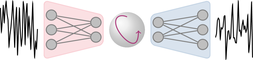
Figure 1: A visual representation of the SyCo-AE framework. From left to right: full order model eq. 3 data is encoded into the reduced order space, the reduced order model eq. 5 is evolved on the sphere $S^{r-1}$, and then decoded out by the decoder, into the reconstruction. Both left and right curves in this figure are real data from the Lorenz ’96 model described in section 4.

If we know that the system that we wish to model is chaotic, then, given an encoder that preserves compactness, the reduced order dynamics have to always remain on some compact set. If they do not then our constructed reduced order model did not take advantage of all our available knowledge, which is a violation of our current best understanding of scientific reasoning [18]. This type of violation is often done deliberately for lack of a better solution. Our task, therefore, is to somehow include this knowledge into our reduced order model construction.

A straightforward consequence of this reasoning is that the construction of the autoencoder eq. 1 cannot be performed independently of the construction of the reduced order dynamics eq. 5. We have to not only ensure that the reduced order dynamics produce outputs that are in accordance with the reduced order space induced by the encoder, but also ensure the complement: that the encoder produces outputs that are in accordance to the outputs produced by the reduced order dynamics.

We now formalize the discussion above by defining a few properties, and their straightforward consequences.

Definition 3.1.

Ideally the dynamics in eq. 5 evolve in a way such that the final state is always in the reduced order space $u_{i+1}\in\mathbb{U}$, which we term this the strong preservation condition.

We now outline how the strong preservation condition in definition 3.1 could be satisfied when the attractor is known.

Theorem 3.1.

When all the possible data points of the attractor $\mathbb{X}$ are fully known, and $\theta$, $\phi$ and $f$ in the standard autoencoder reduced order model eq. 6 are allowed to have an arbitrary amount of degrees of freedom, then the strong preservation condition in definition 3.1 is preservable.

Proof.

With arbitrary many degrees of freedom, the discrepancy of the propagation $u_{i+1}$ and the dimensionality reduced representation of the truth, $\theta(x_{i+1})$, can be zero almost surely for all $x\in\mathbb{X}$, assuming that the autoencoder eq. 1 and reduced order dynamics eq. 5 found simultaneously. ∎

In practice the attractor, $\mathbb{X}$, is not fully known, and in the small-data problem, the known points might be a biased representation thereof. Therefore, the encoder must practically accept all points in $\mathbb{R}^{n}$ as its input. The set defined by the image of $\mathbb{R}^{n}$ under the encoder, $\theta(\mathbb{R}^{n})=\widehat{\mathbb{U}}$ we call the total reduced order space, as it fully covers all possible inputs to the encoder.

Definition 3.2.

If the reduced order dynamics eq. 5 evolve in a way such that the final state is always in this total reduced order space $u_{i+1}\in\widehat{\mathbb{U}}$, we term this the weak preservation condition.

We now motivate our subsequent discussion with the following trivial result.

Theorem 3.2.

A shallow neural network with one hidden layer,

$$\nu(x)=\boldsymbol{\mathbf{A}}_{2}\,\sigma\!\left(\boldsymbol{\mathbf{A}}_{1}x+\boldsymbol{\mathbf{b}}_{1}\right)+\boldsymbol{\mathbf{b}}_{2},$$ (9)

with continuous activation function $\sigma$, maps compact sets to compact sets.

Proof.

Compactness is preserved by continuous functions, thus the composition of an affine, continuous, and another affine function is itself continuous. ∎

We can attempt to learn $\widehat{\mathbb{U}}$ for a given encoder, and force that the dynamics lie on this set. This is inadequate for one simple reason: there is no guarantee that $\widehat{\mathbb{U}}$ is compact, thus being a poorly positioned solution to the problem of modeling chaotic dynamics.

In this work we aim to solve this problem by turning it on its head: instead of learning $\widehat{\mathbb{U}}$ we instead synthetically assign $\widehat{\mathbb{U}}$ to be some compact lower-dimensional manifold embedded in $\mathbb{R}^{r}$. We can then restrict both the encoder eq. 1 and dynamics eq. 5 to map onto and evolve on this manifold. This type of restriction can be performed through a simple algebraic constraint. We first take the autoencoder reduced order model eq. 6, and augment it,

$$\framebox{$\begin{gathered}u=\theta(x),\quad\widetilde{x}=\phi(u),\\ \frac{\mathrm{d}u}{\mathrm{d}t}=f(u),\quad 0=g(u),\end{gathered}$}$$ (10)

where the addition of the synthetic constraint function $g:\mathbb{R}^{r}\to\mathbb{R}^{s}$ with $s\leq r$ has an effect on both the encoder $\theta$ and on the dynamics $f$. The resulting dynamics define a constrained ordinary differential equation [3]. This synthetically constrained autoencoder (SyCo-AE) is described visually by fig. 1.

The hope is that synthetically constraining the dynamics to a known low dimensional set would act as a source of additional knowledge. This knowledge should guide the neural networks to be a good approximation of the underlying dynamics with significantly fewer data. We can also alternatively think about implicitly defining a constraint in the full space. We conjecture:

Conjecture 3.3.

We approximate a complex, not-yet-known, constraint on the full space, $0=G(x)\approx G(\phi(u))$ for all reduced order states $u$ that satisfy our synthetic constraint $0=g(u)$.

In other words, by introducing a known and simple constraint on the reduced order dynamics, we learn some unknown and complex constraint of the full order dynamics. Note that the range of $G$ and $g$ might not have the same dimension, meaning that the optimal choice of $g$ should somehow be informed by the dimension of the range of the unknown $G$.

One simple way to solve enforce the constraint $g$ in eq. 10 for both the encoded and dynamics is through projection. Given the constraint $g$, we can pose the projection operator as minimizing a cost,

$$\Pi(u)=\operatorname*{arg\,min}_{\widehat{u}}\left\lVert\widehat{u}-u\right\rVert_{2}^{2},\qquad\text{such that}\quad 0=g(\widehat{u}),$$ (11)

which for certain choices of $g$ can have a closed form solution. Given an arbitrary encoder $\widehat{\theta}$, the projected autoencoder is given by,

$$\theta(x)=\Pi\left(\widehat{\theta}(x)\right).$$ (12)

In this work for the solution of all continuous dynamical systems, in the interest of speed, we utilize the projected adaptive time-step explicit trapezoidal rule,

$$\begin{gathered}k_{1}=h_{j}\,f(u_{j}),\quad k_{2}=h_{j}\,f(u_{j}+k_{1}),\\ u_{j+1}=\Pi\left[u_{j}+\frac{1}{2}(k_{1}+k_{2})\right],\quad\widetilde{u}_{j+1}=\Pi\left[u_{j}+k1\right],\end{gathered}$$ (13)

where $h_{j}$ is the internal time-step of the solver, $u_{j+1}$ is the next state at time $t_{j}+h$, $\widetilde{u}_{j+1}$ is the solution of the ‘embedded’ method used to adaptively determine $h_{j}$ through the canonical method described in [14], and the function $\Pi$ from eq. 11 projects the solutions onto the manifold defined by $g$ in eq. 10 or is the identity function for all other methods. The ideas for this method are a simple combination of ideas found in [14, 15, 13, 3].

We now turn our attention to the choice of $\widehat{\mathbb{U}}$, implicitly defined by the constraint $g$ in eq. 10. We list a few properties that are nice to have: (i) $\widehat{\mathbb{U}}$ is a compact (and connected) subset of $\mathbb{R}^{r}$, (ii) its topological dimension [16] is as close to $r$ as possible, and (iii) the projection $\Pi$ in eq. 11 has a closed form solution. One simple candidate for such a set is the sphere $S^{r-1}$, with corresponding constraint and projection of,

$$g(u)=\left\lVert u\right\rVert_{2}-1,\quad\Pi(u)=\frac{u}{\left\lVert u\right\rVert_{2}},$$ (14)

that has topological dimension of $r-1$. We make use of the spherical constraint eq. 14 for the remainder of this work, and table the discussion of other possible constraints for future work.

We organize the data into trajectories, with each trajectory, $\{X_{k}\}_{k=0}^{K}$, consisting of data at times $\{t_{k}\}_{k=0}^{K}$. In order to effectively learn the dynamics we explicitly roll out [39] eq. 10, by explicitly solving the constrained initial value problem during training. The degree to which roll out is performed is determined by the length of the trajectory $K$, thus we term $K$ the roll out parameter. We write $\mathcal{M}_{t_{k}\to t_{k+1}}(u_{k})$ for the solution of the constrained initial value problem eq. 10 with an algorithm such as eq. 13. Note that each trajectory can be of variable length and with variable inter-trajectory time-step, however this idea is not explored in this work.

The cost function, therefore has to take into account four distinct parts: (i) the autoencoder error eq. 1, (ii) the right-invertability condition eq. 2, (iii) the error of the dynamics eq. 10 in the full space (through the decoder), (iv) the error of the dynamics eq. 10 in the reduced order space, required by theorem 3.1. The resulting cost function,

$$\begin{aligned} \left.\ell_{i}(\{t_{k}\},\{X_{k}\})\right|_{W}=&\phantom{+\,\,\omega}\sum_{k=0}^{K}\underbrace{\left\lVert X_{k}-\phi(\theta(X_{k}))\right\rVert^{2}_{2}}_{\text{Autoencoder error}}\,\,+\,\,\omega\sum_{k=0}^{K}\underbrace{\left\lVert\theta(X_{k})-\theta(\phi(\theta(X_{k})))\right\rVert^{2}_{2}}_{\text{Right-inverse error}}\\ &+\phantom{\omega}\sum_{k=1}^{K}e^{-2\lambda(t_{k}-t_{0})}\underbrace{\left\lVert X_{k}-\phi(\mathcal{M}_{t_{0}\to t_{k}}(\theta(X_{0})))\right\rVert^{2}_{2}}_{\text{Full space dynamics error}}\\ &+\upsilon\sum_{k=1}^{K}e^{-2\lambda(t_{k}-t_{0})}\underbrace{\left\lVert\theta(X_{k})-\mathcal{M}_{t_{0}\to t_{k}}(\theta(X_{0}))\right\rVert^{2}_{2}}_{\text{Reduced space dynamics error}}\end{aligned},$$ (15)

is implicitly defined in terms of the neural network weights $W$. The constant $\omega$ manipulated the the right inverse error enabling the autoencoder to be weakly right-invertible eq. 2. A large choice, $\omega=10^{2}$, has been shown [29] to significantly improve the performance of autoencoder-based reduced order models. This value of $\omega$ is used in this work. For chaotic systems, the dominant error of the system grows exponentially on average, thus the errors at different times forward into the model have to be scaled accordingly. This accumulation of the error is regulated by $\lambda$ which can be thought of as the approximation of the largest Lyapunov exponent (LLE) [28] for the given dynamics. For a system that is not chaotic, and which can be exactly reconstructed by a reduced order model of dimension $r$, the LLE can be set to $\lambda=0$, meaning that we assume there is no accumulation of error forward in time, which might not strictly be the case. For chaotic systems, $\lambda$ is either known, or can be tuned as a hyperparameter. Finally, $\upsilon$ is a parameter that scales the loss in the reduced order space with respect to the autoencoder loss.

Taking a collection of $I$ trajectories, $\{\{X_{k}\}_{i}\}_{i=1}^{I}$, the full cost function is the expected value with respect to all the trajectories,

$$\!L(W)=\mathbb{E}\left[\left.\ell_{i}(\{t_{k}\}_{i},\{X_{k}\}_{i})\right\rvert_{W}\right].$$ (16)

4 Numerical Experiments

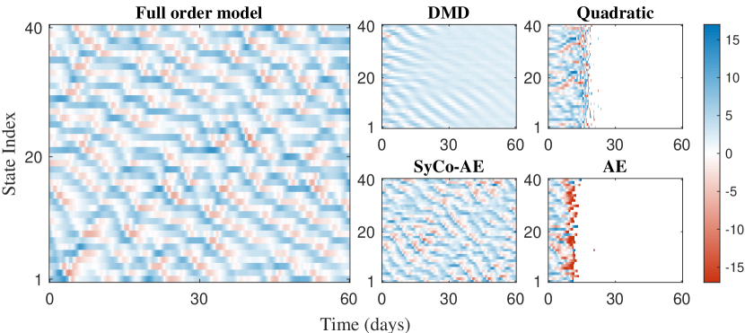
Figure 2: Qualitative representation of the forecasting accuracy of the various ROM methods as compared to the full order Lorenz ’96 model. The same initial condition is taken for all models and propagated for 60 days. The $x$-axis is the time in days, and the $y$-axis is the state-space index of each variable.

(a) $N=100$ data points

(b) $N=500$ data points

(c) $N=1000$ data points

(d) $N=5000$ data points

Figure 3: Medium-range forecasting experiment for the Lorenz ’96 equations and the corresponding ROMs of dimension $r=28$ for various amounts of training data. For each subfigure, the $x$-axis represents the forecasting time in days, ranging from one to 10, and the $y$-axis represents the KL-divergence eq. 18 of the forecasted data points from the truth. Subfigure (a) has results for models trained on $N=100$ data points, (b) on $N=500$ data, (c) on $N=1000$ data, and (d) on $N=5000$ data.

3(a)

For our numerical test case we take the Lorenz ’96 equations [27],

$$\frac{\mathrm{d}x_{j}}{\mathrm{d}t}=-x_{j-1}\left(x_{j-2}-x_{j+1}\right)-x_{j}+F,\quad j\in[1,\dots,40],$$ (17)

with cyclic boundary conditions in $j$, and external force $F=8$. The implementation of the Lorenz ’96 equations used in this work is taken from the ODE Test Problems [34] package.

The Lorenz ’96 equations are a foundational test-bed for algorithms related to numerical weather prediction and data assimilation [33, 2]. They aim to represent a quantity of interest such as pressure along a slice of fixed latitude on the earth. We aim to test the reduced order models’ ability to perform both medium-range (five to 10 days) and long range ($>10$ days) forecasting [19].

While the Lorenz ’96 equations are widely used, it is extremely important to note that it has recently been shown that the equations do not represent a discretization of some partial differential equation model [40].

The Lorenz ’96 model has a known Kaplan-Yorke dimension of $27.1$ and largest Lyapunov exponent of approximately $\lambda\approx 1.6852$, which were independently computed using a method found in [7]. The value of $r$ is generally chosen based on computational limitations, and is thus not treated as a hyperparameter. For these reasons, we focus on the interesting case of $r=28$ for the size of the reduced order model, though preliminary experiments were performed on other values of $r$.

We compare the SyCo-AE method eq. 10 proposed in this work with the standard autoencoder reduced order model eq. 6, with the linear DMD method eq. 7, and with the non-linear Quadratic manifolds eq. 8 method. Both the autoencoder-based methods are trained to minimize the full cost function eq. 16 (made up of eq. 15) using the ADAM [22] method with parameters $\beta_{1}=0.9$ and $\beta_{2}=0.95$, for 1000 epochs, with no minibatching, and a cyclic learning rate scheduler [37] in order to eliminate learning rate as a hyperparameter.

The data collected are trajectories of points collected six hours apart, with each trajectory starting 30 days from the start of the previous, with 0.2 time units corresponding to one day in the model. Not all data points and trajectories are utilized in order to test the methods in the small-data regime.

We train our models on various amounts of data points $N$. We take $N=100$, $N=500$, $N=1000$ and $N=5000$ data points, attempting to range from extremely small, to reasonably large. We take two different values of the roll out factor, $K$ in eq. 15, namely $K=1$ and $K=9$. Note that $N$ does not represent the amount of trajectories that we take, but instead represents the total amount of data points. For example, for $N=100$, a roll out of $K=1$ would correspond to 50 trajectories consisting of two data points each, while a roll out of $K=9$ corresponds to 10 trajectories of 10 points each. In our testing the roll-out factor $K$ did not play a significant role, thus all results are presented with the roll out factor $K=1$, though data for $K=9$ are available.

For both the autoencoder-based methods, we use a fully connected shallow neural network architecture as described in theorem 3.2, for the encoder $\theta$, the decoder $\phi$, and the reduced order dynamics $f$ in eq. 6 and eq. 10. For the hidden layer size we take $H=2000$, though models with $H=500$ were also constructed with slightly worse performance. The encoder for the SyCo-AE method is additionally projected as in eq. 12. As theorem 3.2 requires a continuous activation function, we take the GELU function [17] as our nonlinearity.

All computation was performed on a MacBook M2 Pro laptop, restricting the number of models that could be trained, thus not all hyperparameters could be optimized for.

For the first experiment we look at the qualitative features of all the methods, as compared to the true full order model for a long range forecast of 60 days. We take all models trained on $N=5000$ data point with $K=1$, and $H=2000$ where applicable and forecast a single state outside of the training set.

The results, shown in fig. 2, reveal that the full order model exhibits quasi-periodic behavior, typical of chaotic systems. DMD eq. 7 exhibits decaying behavior, confirmed by the eigenvalues of $\boldsymbol{\mathbf{\Omega}}$ all having negative real part. Quadratic manifold eq. 8 appears to exhibit the correct behavior for approximately 15 days, then appears to catastrophically diverge, which is a known problem in quadratic approximations to dynamical systems [20]. The standard autoencoder approach also appears to have the correct behavior for about five days, but also appears to catastrophically diverge. Only the SyCo-AE method appears to have the same quasi-periodic behavior as the full order model for the full 60 days of the long-range forecast.

In our final experiment we look at the quantitative difference in medium-range forecasting by the reduced order models. There is evidence to suggest that the Lorenz ’96 system is ergodic [9], roughly meaning that any spatial uncertainty is equivalent to temporal uncertainty. We make use of the approximate KL divergence [25, 35] of the data distribution $p$ to the true distribution $q$ in the following numerically stable way,

$$\operatorname{D_{\text{KL}}}\!\left(p\,\middle\|\,q\right)\approx\frac{1}{M}\sum_{x_{i}\sim p,i=1}^{M}\frac{1}{2}\left(\log q(x)-\log p(x)\right)^{2},$$ (18)

with $M$ representing the number of samples taken, and the distributions approximated by Gaussian mixture models computed through kernel density estimation [36].

We propagate $M=10000$ states of the full order and reduced order models forward in time from one to 10 days, and calculate the KL-divergence over time for various data sizes. The results in fig. 3(d) show a clear distinction between the four different methods.

All methods perform poorly for $N=100$ data points, with SyCo-AE eq. 10 being the most stable, though not by much. For $N=500$ and $N=1000$ data points, both DMD eq. 7 and SyCo-AE eq. 10 reach a steady state error, with SyCo-AE having a KL-divergence of an order of magnitude less. The standard autoencoder method is able to produce useful two day forecasts, but then diverges. For $N=5000$ data points the quadratic manifolds method and the standard autoencoder are finally able to produce useful forecasts of about five to six days, but still catastrophically diverge afterwards.

5 Conclusions and Limitations

We provided a new framework for reduced order modeling of chaotic systems with neural networks, synthetically constrained autoencoders (SyCo-AE) eq. 10 that augments a standard autoencoder-based ROM eq. 6 with a synthetic constraint. This simple synthetic constraint in the reduced space stands in as a proxy for an unknown constraint of the system in the full space. Thus, by learning the autoencoder and reduced order dynamics restricted to the simple manifold determined by the synthetic constraint, we implicitly learn the manifold of the full order system.

We test our method on the Lorenz ’96 equations. Results show that the SyCo-AE approach can create stable reduced order models capable of medium-range forecasting that are more accurate than methods that do not enforce a compact constraint on the total reduced order space. Additionally, results show that the amount of data needed to train useful reduced order models is significantly less than other non-linear methods, and seems to be the same as required to train a linear method.

Some of the limitations of this work are as follows. Alternative choices of the the synthetic constraint $g$ are not explored, and a robust justification of the choice of the sphere is absent. A more robust exploration of the tunable hyperparameters and neural network architecture is required. The method in this work was only tested on a simple 40-variable problem, do to computational constraints. A larger exploration of more models, including more geophysically realistic models would strengthen the arguments for or against the current work.

Future work would more formally explore the connection between a spherical synthetic constraint $g$ and spherical embedding [24].

References

- [1] Charu C Aggarwal et al. Neural networks and deep learning. Springer, 10(978):3, 2018.
- [2] Mark Asch, Marc Bocquet, and Maëlle Nodet. Data assimilation: methods, algorithms, and applications. SIAM, 2016.
- [3] Uri M Ascher and Linda R Petzold. Computer methods for ordinary differential equations and differential-algebraic equations, volume 61. Siam, 1998.
- [4] Peter Benner, Mario Ohlberger, Albert Cohen, and Karen Willcox. Model reduction and approximation: theory and algorithms. SIAM, 2017.
- [5] Steven L Brunton and J Nathan Kutz. Data-driven science and engineering: Machine learning, dynamical systems, and control. Cambridge University Press, 2022.
- [6] Steven L Brunton, Joshua L Proctor, and J Nathan Kutz. Discovering governing equations from data by sparse identification of nonlinear dynamical systems. Proceedings of the national academy of sciences, 113(15):3932–3937, 2016.
- [7] Luca Dieci, Michael S Jolly, and Erik S Van Vleck. Numerical techniques for approximating lyapunov exponents and their implementation. Journal of Computational and Nonlinear Dynamics, 6(1), 2011.
- [8] J Doyne Farmer, Edward Ott, and James A Yorke. The dimension of chaotic attractors. Physica D: Nonlinear Phenomena, 7(1-3):153–180, 1983.
- [9] Ibrahim Fatkullin and Eric Vanden-Eijnden. A computational strategy for multiscale systems with applications to Lorenz 96 model. Journal of Computational Physics, 200(2):605–638, 2004.
- [10] Rudy Geelen, Stephen Wright, and Karen Willcox. Operator inference for non-intrusive model reduction with quadratic manifolds. Computer Methods in Applied Mechanics and Engineering, 403:115717, 2023.
- [11] Ian Goodfellow, Yoshua Bengio, and Aaron Courville. Deep learning. MIT press, 2016.
- [12] John Guckenheimer and Philip Holmes. Nonlinear oscillations, dynamical systems, and bifurcations of vector fields, volume 42. Springer Science & Business Media, 2013.
- [13] Ernst Hairer, Marlis Hochbruck, Arieh Iserles, and Christian Lubich. Geometric numerical integration. Oberwolfach Reports, 3(1):805–882, 2006.
- [14] Ernst Hairer, Syvert P Nørsett, and Gerhard Wanner. Solving ordinary differential equations. I, Nonstiff problems. Springer-Vlg, 1991.
- [15] Ernst Hairer and Gerhard Wanner. Solving Ordinary Differential Equations II. Stiff and Differential-Algebraic Problems, volume 14. Springer-Vlg, 01 1996.
- [16] Juha Heinonen et al. Lectures on analysis on metric spaces. Springer Science & Business Media, 2001.
- [17] Dan Hendrycks and Kevin Gimpel. Gaussian error linear units (gelus). arXiv preprint arXiv:1606.08415, 2016.
- [18] Edwin T Jaynes. Probability theory: The logic of science. Cambridge university press, 2003.
- [19] Eugenia Kalnay. Atmospheric modeling, data assimilation and predictability. Cambridge university press, 2003.
- [20] Alan A Kaptanoglu, Jared L Callaham, Aleksandr Aravkin, Christopher J Hansen, and Steven L Brunton. Promoting global stability in data-driven models of quadratic nonlinear dynamics. Physical Review Fluids, 6(9):094401, 2021.
- [21] Anuj Karpatne, Ramakrishnan Kannan, and Vipin Kumar. Knowledge Guided Machine Learning: Accelerating Discovery Using Scientific Knowledge and Data. CRC Press, 2022.
- [22] Diederik P Kingma and Jimmy Ba. Adam: A method for stochastic optimization. arXiv preprint arXiv:1412.6980, 2014.
- [23] Rob Kitchin and Tracey P Lauriault. Small data in the era of big data. GeoJournal, 80:463–475, 2015.
- [24] Antoni A Kosinski. Differential manifolds. Courier Corporation, 2013.
- [25] Solomon Kullback and Richard A Leibler. On information and sufficiency. The annals of mathematical statistics, 22(1):79–86, 1951.
- [26] J Nathan Kutz, Steven L Brunton, Bingni W Brunton, and Joshua L Proctor. Dynamic mode decomposition: data-driven modeling of complex systems. SIAM, 2016.
- [27] Edward N Lorenz. Predictability: A problem partly solved. In Proc. Seminar on predictability, volume 1, 1996.
- [28] Thomas S Parker and Leon Chua. Practical numerical algorithms for chaotic systems. Springer Science & Business Media, 2012.
- [29] Andrey A Popov and Adrian Sandu. Multifidelity ensemble Kalman filtering using surrogate models defined by theory-guided autoencoders. Data-driven modeling and optimization in fluid dynamics: From physics-based to machine learning approaches, 16648714:41, 2023.
- [30] Andrey A Popov, Arash Sarshar, Austin Chennault, and Adrian Sandu. A meta-learning formulation of the autoencoder problem. arXiv preprint arXiv:2207.06676, 2022.
- [31] Tong Qin, Kailiang Wu, and Dongbin Xiu. Data driven governing equations approximation using deep neural networks. Journal of Computational Physics, 395:620–635, 2019.
- [32] David Rand. The topological classification of lorenz attractors. In Mathematical Proceedings of the Cambridge Philosophical Society, volume 83, pages 451–460. Cambridge University Press, 1978.
- [33] Sebastian Reich and Colin Cotter. Probabilistic forecasting and Bayesian data assimilation. Cambridge University Press, 2015.
- [34] Steven Roberts, Andrey A Popov, and Adrian Sandu. ODE test problems: a MATLAB suite of initial value problems. arXiv preprint arXiv:1901.04098, 2019.
- [35] John Schulman. Approximating KL divergence, 2020.
- [36] Bernard W Silverman. Density estimation for statistics and data analysis, volume 26. CRC press, 1986.
- [37] Leslie N Smith. Cyclical learning rates for training neural networks. In 2017 IEEE winter conference on applications of computer vision (WACV), pages 464–472. IEEE, 2017.
- [38] Steven H Strogatz. Nonlinear dynamics and chaos with student solutions manual: With applications to physics, biology, chemistry, and engineering. CRC press, 2018.
- [39] Wayne Isaac Tan Uy, Dirk Hartmann, and Benjamin Peherstorfer. Operator inference with roll outs for learning reduced models from scarce and low-quality data. arXiv preprint arXiv:2212.01418, 2022.
- [40] Dirk Leendert van Kekem. Dynamics of the Lorenz-96 model. PhD thesis, University of Groningen, 2018.
- [41] Lilian Weng. From autoencoder to beta-VAE. lilianweng.github.io, 2018.