The two Higgs doublet type-II seesaw model: Naturalness and $\bar{B}\to X_{s}\gamma$ versus heavy Higgs masses

Abstract

We extend the work Ouazghour:2018mld to a more general and detailed analysis through studying the naturalness problem and $B$ physics constraints within the context of two higgs doublets model augmented with a complex scalar triplet field ($2HDMcT$). We first derive the modified Vetman conditions and show that naturalness problem might be evaded at the electroweak scale. Then, we evaluate the branching ratio of $\bar{B}\to X_{s}\gamma$ radiative decay at the Next to leading order. Besides unitarity, boundedness from below constraints and the present collider data from Higgs signal rate measurements, the parameter space of $2HDMcT$ is then revisited to see how the modified Veltman conditions and $\bar{B}\to X_{s}\gamma$ experimental bounds induce significant delimitations. Our analysis shows that the naturalness affects drastically the masses of heavy Higgs $h_{3}$, $A_{2}$, $H_{2}^{\pm}$ and $H^{\pm\pm}$. More specifically, we considered three benchmak scenarios corresponding to $\mu_{2}>20,40,70$ GeV. For $\mu_{2}>40$, we find stringent upper limits on $m_{h_{2}}$, $m_{A_{1}}$ and $m_{H_{1}^{\pm}}$ at $880$, $920$ and $918$ GeV respectively. If, in addition, the measurements of $\bar{B}\to X_{s}\gamma$ decay rate are also considered, the lower masses limits of nonstandard Higgs bosons ($h_{2}$, $h_{3}$, $A_{1}$, $A_{2}$, $H_{1}^{\pm}$, $H_{2}^{\pm}$, $H^{\pm\pm}$) are pushed up to higher values located between $490$ and $750$ GeV. Besides, we also demonstrate that the $\bar{B}\to X_{s}\gamma$ experimental limits can only be accommodated within $2HDMcT$ if two conditions are fullfilled : $\alpha_{1}$ parameter positive and the Higgs mass hierarchy $m_{h_{3}}>m_{H_{2}^{\pm}}>m_{H^{\pm\pm}}$.

I Introduction

Since the discovery by the ATLAS and CMS experiments at the LHC ATLAS:2012yve ; aad2013atlas ; CMS:2012qbp ; chatrchyan2013observation of a particle with properties that are remarkably consistent with the Higgs boson of the Standard Model ($\mathcal{SM}\;$) gunion2018higgs with a mass about $125$ GeV ATLAS:2015yey , ongoing experimental tests of the $\mathcal{SM}\;$theory and its limitations have provided stringent constraints on new physics beyond the Standard Model ($\mathcal{BSM}\;$). Indeed, despite its brilliant success to describe fundamental particle and their interactions, many questions still remain unexplained and/or controversial., e.g. the dark matter existence in the universe, neutrino oscillations and mass hierarchy. Amidst all of that, the naturalness problem Pivovarov:2007dj is also far from being resolved.

It is then legitimate to propose other theoretical perspectives which could confirm the pattern expected from the Brout-Englert-Higgs mechanism and provide a convincing interpretation of new phenomena $\mathcal{BSM}\;$. For the electroweak hierarchy problem, given the absence of supersymmetry at $TeV$ scale, a plethora of novel altenatives have been considered so far, more particularly with an extended Higgs sector. It is known that one has to call upon new physics where the new degrees of freedom in a particular $\mathcal{BSM}\;$model conspire with those of the Standard Model to get rid of the quadratic divergencies modifying the Veltman condition $(VC)$. As examples of such $\mathcal{BSM}\;$approaches, we can cite the $\mathcal{SM}\;$extended with singlet or triplet scalar fields Chabab:2015nel ; Chabab:2018ert ; Grzadkowski:2009bp ; Karahan:2014ola ; Das:2023tna , the two Higgs doublet Darvishi:2017bhf , and the recent analysis within $2HDM$ augmented with a real triplet scalar Ait-Ouazghour:2020slc .

Due to the similarity in the mass generation mechanism between type-II seesaw and the Brout-Englert-Higgs mechanism, the two Higgs double model extension to the type-II seesaw model ($2HDcT$) and its collider phenomenology are quite appealing, displaying some phenomenological characteristics especially different from those emerging in $2HDM$ scalar sector. Apart its broader spectrum than $2HDM$’s one, the doubly charged Higgs the $H^{++}$ is the smoking gun of $2HDcT$. The search for $H^{++}$ is intensively undergoing by ATLAS and CMS, via the decay channels to $4$ leptons. Searches for $H^{++}H^{--}$ and $H_{i}^{+}H_{i}^{-}$, with $i=1,2$, decaying to the same sign di-lepton, are among the most promising discovery channels of this model. Another prospective signal is $pp\to Z/\gamma\to H_{2}^{+}H_{2}^{-}\to H^{++}W^{-}H^{--}W^{+}\to l^{+}l^{+}l^{-}l^{-}+4j$. This process does not show up neither in $2HDM$ nor in the Higgs triplet model ($HTM$). To shed light on the $2HDMcT$ model’s significance with respect to both the $2HDM$ and $HTM$, we have conducted in Ouazghour:2018mld a first study of the production and decays of several Higgs processes. Our calculations of the cross sections and branching ratios, along with the comprehensive analyses of various decay channels have carried out in-depth exploration of the intricate decay modes of $h_{2,3}$ and $A_{1,2}$, with a specific emphasis on the final states $\gamma\gamma$ and $\tau\tau$. The results from the diphoton decay channels of the pseudoscalar Higgs ($A_{1},A_{2}$), revealed significant suppressions in the products of effective cross sections and branching ratios compared to experimental limits. Furtheremore, we have also investigated scenarios involving the production of Higgs pairs, with a focus on the cases where the observed Higgs boson corresponds either to the lighter scalar ($h_{1}$) or to the second lightest scalar ($h_{2}$). On the other hand, besides Higgs phenomenology, interactions between doublet and triplet fields may also induce a strong first order electroweak phase transtion, thus providing conditions for the baryon asymmetry generation via electroweak baryongenesis (see Ramsey-Musolf:2019lsf for more details).

In this paper, we aim to investigate both the naturalness problem and $\bar{B}\to X_{s}\gamma$ decay rate in the context of a two Higgs doublet type-II seesaw model, dubbed $2HDMcT$. Besides explaining neutrino oscillations, this model has also been examined either to deal with the dark matter issue Chen:2014lla , or to perform phenomenological analyses Ouazghour:2018mld ; Chen:2014xva . More precisely, we will first derive the Veltman conditions ($VC$), study how to soften their divergencies to gain insight into $2HDMcT$ parameter space as on the allowed masses of the heavy scalars in the Higgs sector. Next, we will evaluate the $\bar{B}\to X_{s}\gamma$ decay rate at the next to leading order $(NLO)$ and see whether constraints from the $\bar{B}\to X_{s}\gamma$ measurements affect the $2HDMcT$ spectra. Still, it remains to check that the implementation for$mVC$ and $\bar{B}\to X_{s}\gamma$ constraints are consistent with theoretical requirements and experimental data and how they reshape the Higgs spectrum of our model, in comparison with the previous phenomenological analysis reported in Ouazghour:2018mld

This work is organized as follows: In Sec. II, we briefly review the main features of two Higgs Doublet Type-II Seesaw model. In Sec. III, we briefly present the theoretical and experimental constraints. Section IV is devoted to the derivation of the modified Veltman condition ($VC$) in the $2HDMcT$. In Sec. V, we discuss the constraints on the parameter space from $\bar{B}\to X_{s}\gamma$. The analysis and discussion of the results are performed in Sec. VI, with emphasis on the effects of the modified Veltman conditions as well as the constraints from the $\bar{B}\to X_{s}\gamma$ on the heavy Higgs spectrum, essentially on the charged Higgs sector. A summary of our results will be drawn in Sec. VII.

II TYPE II SEESAW MODEL: BRIEF REVIEW

The $2HDMcT$ contains two Higgs doublets $H_{i}$ (i = 1,2) and one colorless scalar field $\Delta$ transforming as a triplet under the $SU(2)_{L}$ gauge group with hypercharge $Y_{\Delta}=2$. In this case, the most general gauge-invariant Lagrangian of $2HDMcT$ is given by,

$$\begin{matrix}\mathcal{L}=\sum_{i=1}^{2}(D_{\mu}{H_{i}})^{\dagger}(D^{\mu}{H_{i}})+Tr(D_{\mu}{\Delta})^{\dagger}(D^{\mu}{\Delta})\vspace*{0.12cm}\\ -V(H_{i},\Delta)+\mathcal{L}_{\rm Yukawa}\end{matrix}$$ (1)

where the covariant derivatives are defined as,

$$D_{\mu}{H_{i}}=\partial_{\mu}{H_{i}}+igT^{a}{W}^{a}_{\mu}{H_{i}}+i\frac{g^{\prime}}{2}B_{\mu}{H_{i}}$$ (2)

$$D_{\mu}{\Delta}=\partial_{\mu}{\Delta}+ig[T^{a}{W}^{a}_{\mu},\Delta]+ig^{\prime}\frac{Y_{\Delta}}{2}B_{\mu}{\Delta}$$ (3)

(${W}^{a}_{\mu}$, $g$), and ($B_{\mu}$, $g^{\prime}$) denoting respectively the $SU(2)_{L}$ and $U(1)_{Y}$ gauge fields and couplings and $T^{a}\equiv\sigma^{a}/2$, with $\sigma^{a}$ ($a=1,2,3$) the Pauli matrices. In terms of the two $SU(2)_{L}$ Higgs doublets $H_{i}$ and the triplet field $\Delta$, the $2HDMcT$ scalar potential is given by Ouazghour:2018mld ; Chen:2014xva :

$$\begin{matrix}V(H_{i},\Delta)&=&m^{2}_{1}\,H_{1}^{\dagger}H_{1}+m^{2}_{2}\,H_{2}^{\dagger}H_{2}-m_{3}^{2}\,H_{1}^{\dagger}H_{2}-m_{12}^{2}\,H_{2}^{\dagger}H_{1}+\frac{\lambda_{1}}{2}(H_{1}^{\dagger}H_{1})^{2}+\frac{\lambda_{2}}{2}(H_{2}^{\dagger}H_{2})^{2}+\lambda_{3}\,H_{1}^{\dagger}H_{1}\,H_{2}^{\dagger}H_{2}\\ &&+\lambda_{4}\,H_{1}^{\dagger}H_{2}\,H_{2}^{\dagger}H_{1}+\frac{\lambda_{5}}{2}*\left[(H_{1}^{\dagger}H_{2})^{2}+(H_{2}^{\dagger}H_{1})^{2}\right]+\lambda_{6}\,H_{1}^{\dagger}H_{1}Tr\Delta^{\dagger}{\Delta}+\lambda_{7}\,H_{2}^{\dagger}H_{2}Tr\Delta^{\dagger}{\Delta}\hskip 34.14322pt\\ &&+[\mu_{1}H_{1}^{T}{i}\sigma^{2}\Delta^{\dagger}H_{1}+\mu_{2}H_{2}^{T}{i}\sigma^{2}\Delta^{\dagger}H_{2}+\mu_{3}H_{1}^{T}{i}\sigma^{2}\Delta^{\dagger}H_{2}+{\rm h.c.}]+\lambda_{8}\,H_{1}^{\dagger}{\Delta}\Delta^{\dagger}H_{1}\hskip 71.13188pt\\ &&+\lambda_{9}\,H_{2}^{\dagger}{\Delta}\Delta^{\dagger}H_{2}+m^{2}_{\Delta}\,Tr(\Delta^{\dagger}{\Delta})+\bar{\lambda}_{8}(Tr\Delta^{\dagger}{\Delta})^{2}+\bar{\lambda}_{9}Tr(\Delta^{\dagger}{\Delta})^{2}\hskip 130.88284pt\end{matrix}$$

where $Tr$ denotes the trace over 2x2 matrices. The triplet $\Delta$ and doublet Higgs H are represented by,

$$\Delta = \left(\begin{array}[]{cc}\delta^{+}/\sqrt{2}&\delta^{++}\\ (v_{t}+\delta^{0}+i\eta_{0})/\sqrt{2}&-\delta^{+}/\sqrt{2}\\ \end{array}\right)$$ (6)

$$H_{1} = \left(\begin{array}[]{c}\phi_{1}^{+}\\ \phi^{0}_{1}\\ \end{array}\right){,}~{}~{}~{}H_{2}=\left(\begin{array}[]{c}\phi_{2}^{+}\\ \phi^{0}_{2}\\ \end{array}\right)$$ (11)

with $\phi^{0}_{1}=(v_{1}+\rho_{1}+i\eta_{1})/\sqrt{2}$ and $\phi^{0}_{2}=(v_{2}+\rho_{2}+i\eta_{2})/\sqrt{2}$. After the spontaneous electroweak symmetry breaking, the Higgs doublets and triplet fields acquire their vacuum expectation values, respectively dubbed $v_{1}$, $v_{2}$ and $v_{t}$, and eleven physical Higgs states appear, namely: three CP-even neutral Higgs bosons $(H_{1},H_{2},H_{3})$, four simply charged Higgs bosons $(H_{1}^{\pm},H_{2}^{\pm})$, two CP odd Higgs $(A_{1},A_{2})$, and finally two doubly charged Higgs bosons $H^{\pm\pm}$. For detail see Ouazghour:2018mld .

III THEORETICAL AND EXPERIMENTAL CONSTRAINTS

The allowed $2HDMcT$ parameter space must generally obey to many theoretical and experimental constraints. These constraints include vacuum stability, unitarity and perturbativity, in addition to experimental constraints and exclusion limits especially originating from the measurements of Higgs boson properties, flavor-changing neutral currents and electroweak precision observables. These are smoking guns to probe imprints of new physics within the model. Hereafter, we provide a brief description of all constraints invoked to delimit the model parameter space and used in our subsequent analysis Ouazghour:2018mld :

• Unitarity: The scattering processes have to be unitary.

• Perturbativity: The quartic couplings of scalar potential must obey the following conditions:$|\lambda_{i}|<8\pi$ for each $i=1,..,9$ and $|\bar{\lambda}_{i}|<8\pi$ for $i=8,9$.

• Vacuum stability : Positivity in any direction of fields $\Phi_{i}$, $\Delta$ and boundedness from below $BFB$.

• Experimental Higgs boson exclusion limits: Existing exclusion limits at the 95% confidence level from Higgs searches at LEP, LHC, and Tevatron have been enforced via HiggsBounds-5.10.1 bechtle2010higgsbounds ; bechtle2011higgsbounds ; bechtle2014higgsbounds ; bechtle2020higgsbounds ; bahl2022testing .

• SM-like Higgs boson discovery: Compatibility with the measurements of the Higgs signal rate from various searches at the $95\%$ confidence level, essentially from the LHC Run 2. Here we used HiggsSignals-2.6.1 bechtle2014higgssignals ; bechtle2021higgssignals .

• The electroweak precision observables $(EWPO)$: Generally, the additional scalars in a model introduce extra correctionsto the gauge boson self energy diagrams, which affect electroweak precision observables $(EWPO)$, as the oblique parameters $S$, $T$ and $U$. Accordingly the new charged, doubly charged and neutral bosons in $2HDMcT$ yield corrections to the analytic formulas of $S$ and $T$. To estimate the oblique parameters in the present model, we use the prescription adopted in Lavoura:1993nq where for simplicity the general expressions of $S$, $T$ and $U$ where established by assuming that the complex scalar multiplet with a small vacuum expectaion value and no coupling to the other scalars of the theory. This translates in $2HDMcT$ to $v_{t}\leq 1$ GeV with the following rotation matrix elements: $\alpha_{2}$ and $\alpha_{3}$ almost vanishing, while $C_{33}$ (charged) and $O_{33}$ tend to $\approx 1$. In this context, the doublets and triplet fields decouple. This means that major contributions to the physical fields $h_{3}$, $A_{2}$, $H^{\pm}_{2}$ and $H^{\pm\pm}$ originate from triplet fields while the dominat contributions to $h_{1}$, $h_{2}$, $A_{1}$ and $H_{1}^{\pm}$ are from doublet fields. Using the general expressions presented in Grimus:2007if ; Grimus:2008nb ; Lavoura:1993nq , we readily calculate the new contribution to the $S$ and $T$ parameters from the new scalars in $2HDMcT$ as,

  $$T = \frac{1}{16\pi m_{W}^{2}s_{W}^{2}}(F(m_{H^{\pm\pm}}^{2},m_{H^{\pm}_{2}}^{2})+F(m_{H^{\pm}_{2}}^{2},m_{h_{3}}^{2})+{\cal R}_{21}^{2}F(m_{H_{1}^{\pm}}^{2},m_{h_{1}}^{2})$$ (12)

  $$+ {\cal R}_{22}^{2}F(m_{H_{1}^{\pm}}^{2},m_{h_{2}}^{2})+F(m_{H_{1}^{\pm}}^{2},m_{A_{1}}^{2})-{\cal R}_{21}^{2}F(m_{h_{1}}^{2},m_{A_{1}}^{2})-{\cal R}_{22}^{2}F(m_{h_{2}}^{2},m_{A_{1}}^{2})$$

  $$+ 3({\cal R}_{11}^{2}(F(m_{Z}^{2},m_{h_{1}}^{2})-F(m_{W}^{2},m_{h_{1}}^{2}))+{\cal R}_{12}^{2}(F(m_{Z}^{2},m_{h_{2}}^{2})-F(m_{W}^{2},m_{h_{2}}^{2})))$$

  $$- 3(F(m_{Z}^{2},m_{h_{ref}}^{2})-F(m_{W}^{2},m_{h_{ref}}^{2})))$$

  and

  $$S= \frac{1}{24\pi}[(2s_{W}^{2}-1)^{2}G(m_{H_{1}^{+}}^{2},m_{H_{1}^{+}}^{2},m_{Z}^{2})+{\cal R}_{21}^{2}G(m_{h_{1}}^{2},m_{A_{1}}^{2},m_{Z}^{2})$$

  $$+({\cal R}_{11}^{2}+{\cal R}_{21}^{2})\ln(m_{h_{1}}^{2})+({\cal R}_{12}^{2}+{\cal R}_{22}^{2})\ln(m_{h_{2}}^{2})+\ln(m_{A_{1}}^{2}))$$

  $$+{\cal R}_{22}^{2}G(m_{h_{2}}^{2},m_{A_{1}}^{2},m_{Z}^{2})-2\ln(m_{H_{1}^{\pm}}^{2})-\ln(m_{h_{ref}}^{2})$$

  $$+{\cal R}_{11}^{2}\hat{G}(m_{h_{1}^{2}},m_{Z}^{2})+{\cal R}_{12}^{2}\hat{G}(m_{h_{2}}^{2},m_{Z}^{2})-\hat{G}(m_{h_{ref}}^{2},m_{Z}^{2})]+$$ (13)

  $$\frac{1}{3\pi}\bigg{[}-\ln\left(\frac{m_{H^{\pm\pm}}^{2}}{m_{h_{3}}^{2}}\right)+\frac{1}{2}\xi\left(\frac{m_{h_{3}}^{2}}{m_{Z}^{2}}\right)+\frac{(1-2s^{2}_{w})^{2}}{2}\xi\left(\frac{m_{H^{\pm\pm}}^{2}}{m_{Z}^{2}}\right)$$

  $$+\frac{s^{4}_{w}}{2}\xi\left(\frac{m_{H_{2}^{\pm}}^{2}}{m_{Z}^{2}}\right)\bigg{]}$$ (14)

  with

  $${\cal R}_{11}=C_{11}R_{11}+C_{12}R_{12}$$ (15)

  $${\cal R}_{22}=C_{21}R_{21}+C_{22}R_{22}$$ (16)

  $${\cal R}_{12}=C_{11}R_{21}+C_{12}R_{22}$$ (17)

  $${\cal R}_{21}=C_{21}R_{11}+C_{22}R_{12}$$ (18)

  and $m_{h_{ref}}$ is the reference mass of the neutral SM Higgs and $s_{w}=sin(\theta_{w})$ where $\theta_{w}$ is the Weinberg angle. The explicit forms of these functions, $F\left(x,y\right)$, $G\left(I,J,Q\right)$, $\hat{G}\left(I,Q\right)$ and $\xi(x)$ are given in grimus801oblique ; Lavoura:1993nq .

  $$F\left(x,y\right)\equiv\left\{\begin{array}[]{ll}{\displaystyle\frac{x+y}{2}-\frac{xy}{x-y}\,\ln{\frac{x}{y}}}&\Leftarrow\ x\neq y,\\[8.53581pt] 0&\Leftarrow\ x=y.\end{array}\right.$$ (19)

  $$G\left(I,J,Q\right)= -\frac{16}{3}+\frac{5\left(I+J\right)}{Q}-\frac{2\left(I-J\right)^{2}}{Q^{2}}$$

  $$+\frac{3}{Q}\left[\frac{I^{2}+J^{2}}{I-J}-\frac{I^{2}-J^{2}}{Q}+\frac{\left(I-J\right)^{3}}{3Q^{2}}\right]\ln{\frac{I}{J}}+\frac{r}{Q^{2}}\,f\left(t,r\right).$$ (20)

  If $I=J$, $G(I,J,Q)$ is :

  $$G\left(I,J,Q\right) = -\frac{16}{3}+\frac{16}{Q}I+\frac{r}{Q^{3}}\,f\left(t,r\right)$$

  and :

  $$f\left(t,r\right)\equiv\left\{\begin{array}[]{lcl}{\displaystyle\sqrt{r}\,\ln{\left|\frac{t-\sqrt{r}}{t+\sqrt{r}}\right|}}&\Leftarrow&r>0,\\[8.53581pt] 0&\Leftarrow&r=0,\\[5.69054pt] {\displaystyle 2\,\sqrt{-r}\,\arctan{\frac{\sqrt{-r}}{t}}}&\Leftarrow&r<0.\end{array}\right.$$ (24)

  with :

  $$t\equiv I+J-Q\quad\mbox{and}\quad r\equiv Q^{2}-2Q\left(I+J\right)+\left(I-J\right)^{2}$$

  $$\hat{G}\left(I,Q\right) = -\frac{79}{3}+9\,\frac{I}{Q}-2\,\frac{I^{2}}{Q^{2}}+\bigg{(}12-4\,\frac{I}{Q}+\frac{I^{2}}{Q^{2}}\bigg{)}\frac{f\left(I,I^{2}-4IQ\right)}{Q}$$ (25)

  $$+ \bigg{(}-10+18\,\frac{I}{Q}-6\,\frac{I^{2}}{Q^{2}}+\frac{I^{3}}{Q^{3}}-9\,\frac{I+Q}{I-Q}\bigg{)}\ln{\frac{I}{Q}}.$$

  and

  $$\xi(x) =12\left(\frac{4}{9}-\frac{4}{3}x+\frac{1}{12}(4x-1)f(x)\right),$$ (26)

  $$f(x) =\left\{\begin{aligned} &-4\sqrt{4x-1}\arctan\frac{1}{\sqrt{4x-1}},\quad\text{for }4x>1,\\ &\sqrt{1-4x}\ln\frac{2x-1+\sqrt{1-4x}}{2x-1-\sqrt{1-4x}},\quad\text{for }4x\leq 1,\end{aligned}\right.$$

  By assuming that $U=0$, analysis of the precision electroweak data with the new PDG mass of the $W$ boson yields ParticleDataGroup:2020ssz :

  $$S^{exp}=0.05\pm 0.08,\;\;\;T^{exp}=0.09\pm 0.07\;\;\;and\;\;\;\rho_{ST}=+0.92.$$ (27)

  where $\rho_{ST}$ corresponds to the correlation coefficient in the $\chi_{ST}^{2}$ analysis. Next, we use the following $\chi^{2}_{ST}$ test where only points that are within $95\%$ confidence level (C.L.) of the PDG measurements are considered,
  

  $$\chi^{2}_{ST} = \frac{1}{\hat{\sigma_{T}}^{2}_{1}(1-\rho_{ST}^{2})}(T-T^{exp})^{2}+\frac{1}{\hat{\sigma_{S}}^{2}_{1}(1-\rho_{ST}^{2})}(S-S^{exp})^{2}$$ (28)

  $$- \frac{2\rho_{ST}}{\hat{\sigma}_{T}\hat{\sigma}_{S}(1-\rho_{ST}^{2})}(T-T^{exp})(S-S^{exp})\leq R^{2}\,,$$

  with $R^{2}=2.3$, $5.99$ and $11.83$ at $68.3\%$, $95\%$ and $99.7\%$ CLs, respectively and $\hat{\sigma}_{T}$, $\hat{\sigma}_{S}$ are one-sigma errors.

IV THE MODIFIED VELTMAN CONDITIONS

As it is known, the new degrees of freedom in any new physics models spectrum conspire with the $SM$ ones in order to soften the quadratic divergencies. The Veltman conditions (VC) are then modified and naturalness problem gets under control within the model parameter space. So, to derive the Veltman conditions in $2HDMcT$, one just has to collect the quadratic divergencies of the Higgs self-energies in terms of the original fields, namely the doublet $\Phi_{1}$ , $\Phi_{2}$ and triplet $\Delta$, without spontaneous breaking of the $SU(2)\times U(1)$ gauge symmetry Veltman:1980mj . There are various ways to do that, however the safest way is to use the dimensional regularization siegel1979supersymmetric ; einhorn1992effective ; al1992quadratic as this approach guarantees both gauge Lorentz invariances. Besides, we performed this calculation in a general linear $R_{\xi}$ gauge and verified that the results obtained are entirely free of $\xi$-parameter as required. To work out these quadratic divergencies, we followed exactly the calculation steps described in our previous work on the two Higgs doublet model extended by a real triplet scalar field $\Delta$ Ait-Ouazghour:2020slc and in Newton:1993xc ; newton1994can ; Al-Sarhi:1990nmv ; Einhorn:1992um . Throughout these calculations, we used the following convenient notation,

• $(\Phi)_{p}$ and $(\Delta)_{q}$ denotes the p-component of the doublets and q-component of the triplet fields.

• $I_{11}(I_{22})$ as the quadratically divergent part of the two-point functions with either the upper or lower components of $\Phi_{1}$ ($\Phi_{2}$) fields, on both external lines of the relevant Feynman Diagrams. Similarly, we label $I_{33}$ for the triplet two-point functions, with one of $\Delta$ components on external lines.

To derive the final results in symmetry unbroken phase, it is necessary to summarize all possible schemes, taking only the coefficients of divergent parts in $I_{ij}$, leading to:

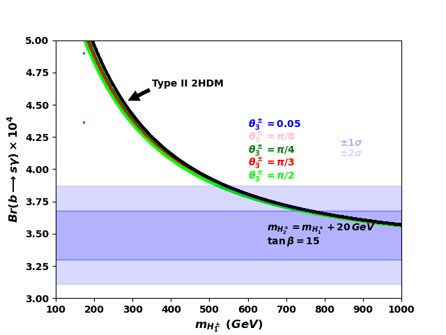
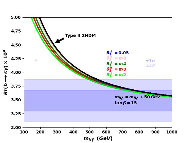
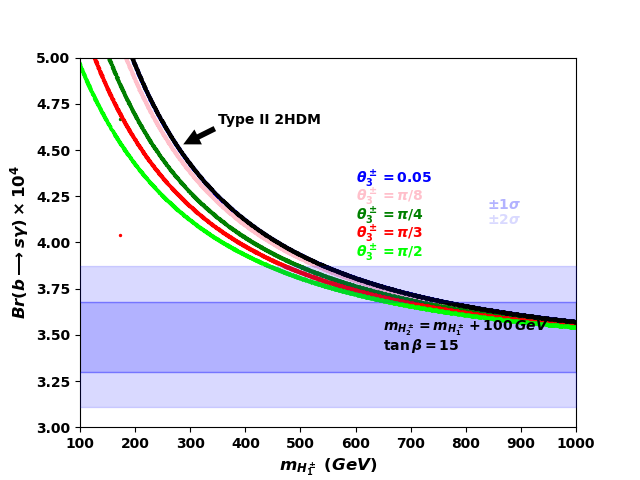
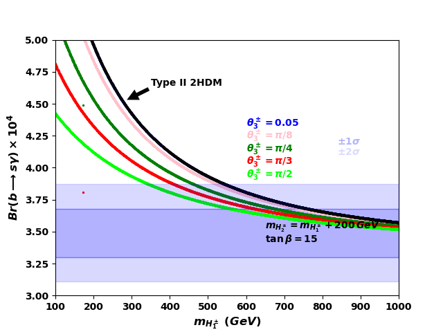
Figure 1: Predictions for the branching ratio of $B\rightarrow X_{s}\gamma$ in $2HDMcT$ type II as a function of $m_{H_{1}^{\pm}}$. First and second column panels correspond respectively to $\tan\beta=1\;and\;\;15$, with $m_{H_{2}^{\pm}}-m_{H_{1}^{\pm}}=20,\;50,\;100$ and $200$ GeV.

$$I_{11} \rightarrow 3/4g^{2}+1/4g^{{}^{\prime}2}+3\lambda_{1}+2\lambda_{3}+\lambda_{4}$$ (29)

$$+(3\lambda_{6}+\frac{3}{2}\lambda_{8})-\left(\frac{\sqrt{2}}{v}\right)^{2}\frac{m_{D}^{2}}{cos^{2}\beta}$$

$$I_{22} \rightarrow 3/4g^{2}+1/4g^{{}^{\prime}2}+3\lambda_{2}+2\lambda_{3}+\lambda_{4}$$ (30)

$$+(3\lambda_{7}+\frac{3}{2}\lambda_{9})-\left(\frac{\sqrt{2}}{v}\right)^{2}\frac{m_{U}^{2}}{sin^{2}\beta}$$

$$I_{33} \rightarrow 2g^{2}+g^{{}^{\prime}2}+2(\lambda_{6}+\lambda_{7})+\lambda_{8}+\lambda_{9}+8\bar{\lambda}_{8}+6\bar{\lambda}_{9}$$ (31)

where $m^{2}_{D}=m^{2}_{e}+m^{2}_{\mu}+m^{2}_{\tau}+3(m^{2}_{d}+m^{2}_{s}+m^{2}_{b})$, $m^{2}_{U}=3(m^{2}_{u}+m^{2}_{c}+m^{2}_{t})$ and $v^{2}=v_{1}^{2}+v_{2}^{2}+2v_{t}^{2}$ is the square of the Standard Model vacuum expectation value $(\approx 246GeV)$.

Finally, thanks to the relations $\cos\beta=\frac{v_{1}}{v_{0}}$, $\sin\beta=\frac{v_{2}}{v_{0}}$, $m_{W}=\frac{gv}{2}$, $e=g\sin\theta_{weinberg}$ and $g^{{}^{\prime}}=g\tan\theta_{weinberg}$, the tadpoles equations in the broken phase are thoroughly recovered:

$$\delta T_{d_{1}} = \frac{m_{W}^{2}}{v^{2}}\left(2+\frac{1}{c_{w}^{2}}\right)+3\lambda_{1}+2\lambda_{3}+\lambda_{4}+(3\lambda_{6}+\frac{3}{2}\lambda_{8})$$ (32)

$$- \left(\frac{\sqrt{2}}{v}\right)^{2}\frac{m_{D}^{2}}{cos^{2}\beta}$$

$$\delta T_{d_{2}} = \frac{m_{W}^{2}}{v^{2}}\left(2+\frac{1}{c_{w}^{2}}\right)+3\lambda_{2}+2\lambda_{3}+\lambda_{4}+(3\lambda_{7}+\frac{3}{2}\lambda_{9})$$ (33)

$$- \left(\frac{\sqrt{2}}{v}\right)^{2}\frac{m_{U}^{2}}{sin^{2}\beta}$$

and for the triplet:

$$\delta T_{t} = 4\frac{m_{W}^{2}}{v^{2}}\left(1+\frac{1}{c_{w}^{2}}\right)+2(\lambda_{6}+\lambda_{7})+\lambda_{8}+\lambda_{9}+8\bar{\lambda}_{8}+6\bar{\lambda}_{9}$$ (34)

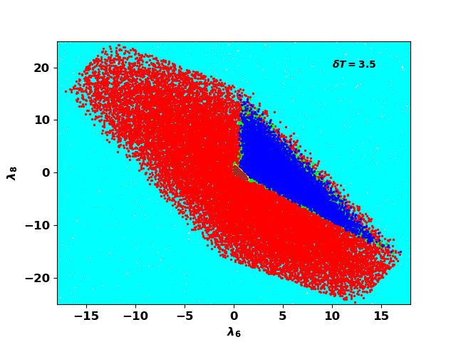
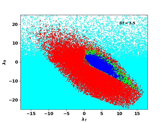
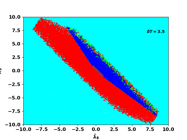
Figure 2: The allowed regions in ($\lambda_{6}$, $\lambda_{8}$) (left), ($\lambda_{7}$, $\lambda_{9}$) (middle) and ($\bar{\lambda}_{8}$, $\bar{\lambda}_{9}$) (right) by imposing $C_{1}$ (blue), combined $C_{1}$ and $EWPO$ (plum), $C_{2}$ (yellow) and $C_{3}$ (brown) constraints

At this point, several comments and remarks are in order:

• The potential parameter $\lambda_{1}$ is missing in $\delta T_{d_{2}}$, and similarly $\lambda_{2}$ is absent in $\delta T_{d_{1}}$, while $\delta T_{t}$ excludes both $\lambda_{1}$ and $\lambda_{2}$. This can be explained via Eqs. (32, 33, 34) which show that $\lambda_{1}$ and $\lambda_{2}$ couple solely to $H_{1}$ and $H_{2}$ field resepctively. The couplings $\bar{\lambda}_{8}$ and $\bar{\lambda}_{9}$, originating from the triplet scalar, rather manifest themselves in $\delta T_{t}$.

• The couplings $\lambda_{6}$ and $\lambda_{8}$ ($\lambda_{7}$ and $\lambda_{9}$) do not appear in $\delta T_{d_{2}}$ ($\delta T_{d_{1}}$) since they are only related to $H_{1}$ ($H_{2}$) potential terms.

• The Veltman conditions for the Higgs Triplet Model with $Y=2$ reported in Chabab:2015nel can be recovered when some of the couplings vanish, and $v_{1}$ traded for $v_{d}$ in Eqs.(32, 33, 34). Similarly, the Veltman conditions in $2HDM$ Darvishi:2017bhf ; Grzadkowski:2009mj ; Grzadkowski:2010dn ; drozd2012multi ; Bazzocchi:2012de ; Masina:2013wja ; Chakraborty:2014oma ; Biswas:2014uba ; chowdhury2015global are reproduced when the couplings that fingerprint the scalar triplet in the Lagrangian, namely $\lambda_{6}$, $\lambda_{7}$, $\lambda_{8}$, $\lambda_{9}$, $\bar{\lambda}_{8}$, $\bar{\lambda}_{9}$, are removed from Eqs. (32, 33, 34).

To proceed with the implementation of the $VC$’s in the parameter space and in the subsequent scans one usually assumes that the deviation $\delta T$ should not exceed the Higgs mass scale (Veltman’s theorem $\delta m_{H}^{2}/m_{H}^{2}\ll 1$). To determine the most appropriate values of $\delta T$ for the phenomenological analysis, we first allowed $\delta T$ to lie within the conservative range of $0.1$ to $4$ GeV. Then we identified the following features:

• Naturalness constraints are stronger than the other theoretical conditions.

• The deviations $\delta T$ must exceed $2.6$ GeV to maintain a viable model.

• The sample of generated points that satisfy all constraints, including $VC$, is significant when $\delta T$ is about $3.5$ GeV.

  Therefore, to balance between these two requirements (Veltman’s theorem and the model viability), we assume thereafter that the deviations in $\delta T$ should not exceed $3.5$ GeV.

V CONSTRAINTS FROM $B\to X_{s}\gamma$

The $B\to X_{s}\gamma$ decay is an important process for constraining new physics, as it is highly sensitive to physics beyond the Standard Model. Therefore, any model that aims to predict a light charged Higgs boson must also be consistent with the experimental constraints on this decay. This feature has been observed in several models with charged Higgs states, such as the two Higgs doublet model extended by a real triplet scalar field Ait-Ouazghour:2020slc where a charged Higgs with a mass smaller than the $200$ GeV has been predicted. In this section, following borzumati1998two , we investigate whether the $2HDMcT$ model has the potential to accommodate a light charged Higgs, while being consistent with $BR(\bar{B}\to X_{s}\gamma)$ decay experimental limits.

From Belle Belle:2014nmp , Babar BaBar:2007yhb ; BaBar:2012fqh ; BaBar:2012eja and CLEO CLEO:2001gsa measurements extrapolated down to $E_{0}=1.6$ GeV, the experimental world average evaluated by HFAG  HFLAV:2022pwe reads:

$${\cal BR}(\overline{B}\to X_{s}\gamma)|_{E_{\gamma}>1.6\mathrm{~{}GeV}}=\left(3.40\pm 0.17\right)\times 10^{-4}$$ (35)

In this context, as a first step towards exploring the viability of the $2HDMcT$, we first calculate the $BR(\bar{B}\to X_{s}\gamma)$ decay rate at $NLO$ where the two singly charged Higgs states are both involved.

One can write the branching ratio of the radiative $B\to X_{s}\gamma$ decay process at $NLO$ in QCD as:

$$BR(B\rightarrow X_{s}\gamma)=\frac{\Gamma(B\rightarrow X_{s}\gamma)}{\Gamma_{SL}}BR_{SL}$$ (36)

where $BR_{SL}$ is the measured semileptonic branching ratio, whereas the semileptonic decay width $\Gamma_{SL}$ is expressed by:

$$\Gamma_{SL}=\frac{G_{F}^{2}}{192\pi^{3}}|V_{cb}|^{2}m_{b}^{5}g(z)\left(1-\frac{2\alpha_{s}(\bar{\mu}_{b})}{3\pi}f(z)+\frac{\delta^{NP}_{SL}}{m_{b}^{2}}\right);\;\;\;\;z=\frac{m_{c}^{2}}{m_{b}^{2}}$$ (37)

The phase space function $g(z)$, the (approximated) QCD–radiation function $f(z)$ and the non–perturbative correction $\delta^{NP}_{SL}$ are defined in borzumati1998two . The decay $\Gamma(B\rightarrow X_{s}\gamma)$ at $NLO$ is given by:

$$\Gamma(B\rightarrow X_{s}\gamma)=\frac{G_{F}^{2}}{32\pi^{4}}|V_{ts}^{\star}V_{tb}|^{2}\alpha_{em}m_{b}^{5}\left(|{\overline{D}}|^{2}+A+\frac{\delta^{{\scriptscriptstyle NP}}_{\gamma}}{m_{b}^{2}}|C_{7}^{0,\,{\rm eff}}(\mu_{b})|^{2}\right.$$

$$\left.+\frac{\delta^{{\scriptscriptstyle NP}}_{c}}{m_{c}^{2}}{\rm Re}\left(\left[C_{7}^{0,\,{\rm eff}}(\mu_{b})\right]^{*}\left(C_{2}^{0,\,{\rm eff}}(\mu_{b})-\frac{1}{6}C_{1}^{0,\,{\rm eff}}(\mu_{b})\right)\right)\right).$$

where the amplitudes $A$ and $\bar{D}$ read as,

$$A=\frac{\alpha_{s}(\mu_{b})}{\pi}\sum_{i,j=1;i\leq j}^{8}Re\left(C^{0,eff}_{i}(\mu_{b})[C^{0,eff}_{j}(\mu_{b})]^{*}f_{ij}\right)$$ (39)

$$\bar{D}=C^{0,eff}_{7}(\mu_{b})+\frac{\alpha_{s}(\mu_{b})}{4\pi}\left(C^{1,eff}_{7}+V(\mu_{b})\right)$$ (40)

with $C^{0,eff}_{7}(\mu_{b})$ and $C^{1,eff}_{7}(\mu_{b})$ defined as :

$$C^{0,eff}_{7}(\mu_{b})=\eta^{\frac{16}{23}}C^{0,eff}_{7}(\mu_{w})+\frac{8}{3}(\eta^{\frac{14}{23}}-\eta^{\frac{16}{23}})C^{0,eff}_{8}(\mu_{w})+\sum_{i=1}^{8}h_{i}\eta^{a_{i}}$$ (41)

$$C^{1,\,{\rm eff}}_{7}(\mu_{b}) = \eta^{\frac{39}{23}}C^{1,\,{\rm eff}}_{7}(\mu_{\scriptscriptstyle W})+\frac{8}{3}\left(\eta^{\frac{37}{23}}-\eta^{\frac{39}{23}}\right)C^{1,\,{\rm eff}}_{8}(\mu_{\scriptscriptstyle W})$$ (42)

$$+ \left(\frac{297664}{14283}\eta^{\frac{16}{23}}-\frac{7164416}{357075}\eta^{\frac{14}{23}}+\frac{256868}{14283}\eta^{\frac{37}{23}}\right)C^{0,\,{\rm eff}}_{8}(\mu_{\scriptscriptstyle W})$$

$$- \frac{6698884}{357075}\eta^{\frac{39}{23}}C^{0,\,{\rm eff}}_{8}(\mu_{\scriptscriptstyle W})+\,\frac{37208}{4761}\left(\eta^{\frac{39}{23}}-\eta^{\frac{16}{23}}\right)C^{0,\,{\rm eff}}_{7}(\mu_{\scriptscriptstyle W})$$

$$+ \sum_{i=1}^{8}\left(e_{i}\,\eta\,C^{1,\,{\rm eff}}_{4}(\mu_{\scriptscriptstyle W})+(f_{i}+k_{i}\eta)\,C^{0,\,{\rm eff}}_{2}(\mu_{\scriptscriptstyle W})\right)\eta^{a_{i}}\,,$$

$$+ \sum_{i=1}^{8}l_{i}\,\eta\,C^{1,\,{\rm eff}}_{1}(\mu_{\scriptscriptstyle W})\eta^{a_{i}}\,,$$

where $V(\mu_{b})$, $\eta$, $C^{0,eff}_{1}(\mu_{w})$, $C^{0,eff}_{2}(\mu_{w})$, $C^{1,eff}_{1}(\mu_{w})$, $C^{1,eff}_{4}(\mu_{w})$, and the vectors $a_{i}$, $h_{i}$, $e_{i}$, $f_{i}$, $k_{i}$, $l_{i}$ are reported in borzumati1998two .

The effective Wilson coefficient $C^{1,eff}_{7}(\mu_{w})$ at the $\mu_{W}$ scale is given by:

$$C^{1,eff}_{7}(\mu_{w})=C^{1,eff}_{7,SM}+\sum_{a=1,2}|Y_{a}|^{2}C^{1,eff}_{7,Y_{a}Y_{a}}+X_{a}Y_{a}^{*}C^{1,eff}_{7,X_{a}Y_{a}}$$ (43)

The coefficient $C_{7,SM}^{0}(\mu_{w})$ is a function of $x=m^{2}_{t}/M_{w}^{2}$ , while $C^{1,eff}_{7,Y_{a}Y_{a}}(\mu_{w})$ and $C^{1,eff}_{7,X_{a}Y_{a}}(\mu_{w})$ $(a=1,\;2)$ are functions of $y=m_{t}^{2}/m^{2}_{H^{\pm}_{a}}$ ($H^{\pm}_{a}=H^{\pm}_{1},\;H^{\pm}_{2}$); their explicit forms are summarized in borzumati1998two . In our model, the couplings $Y_{1}$, $Y_{2}$, $X_{1}$ and $X_{2}$ read as:

$$Y_{1}=\frac{C_{22}}{\sin\beta},\;\;Y_{2}=\frac{C_{32}}{\sin\beta},\;\;X_{1}=-\frac{C_{21}}{\cos\beta}\;\;and\;\;X_{2}=-\frac{C_{31}}{\cos\beta}$$ (44)

where the elements of rotation matrix $C_{ij}$ can be collected from Ouazghour:2018mld ,

Now that we have defined all the necessary ingredients, we can examine the branching ratio of $B\rightarrow X_{s}\gamma$ radiative decay at $NLO$ within $2HDMcT$.

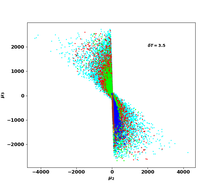
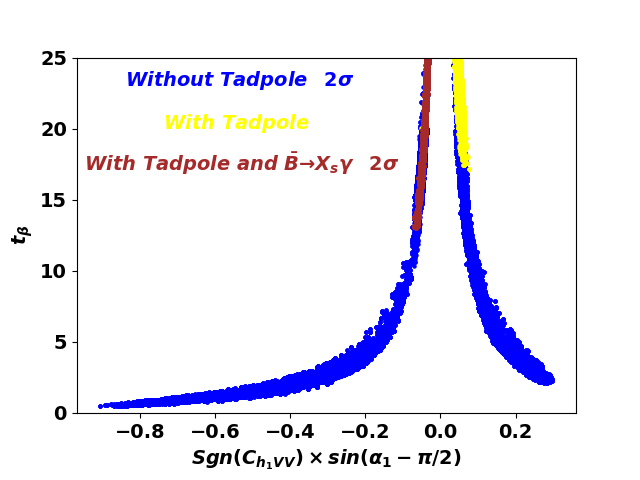
Figure 3: The allowed regions in the planes $\mu_{2}$ vs $\mu_{3}$ (left) and ($sgn(C_{V}^{h_{1}})\sin(\alpha_{1}-\pi/2)$, $\tan\beta$) (right). All theoretical and experimental constraints are taken into account with color captions similar to Fig [2].

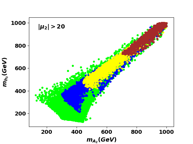
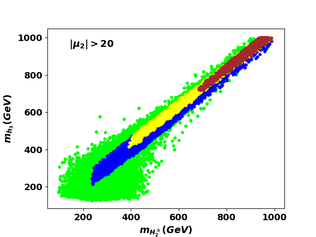
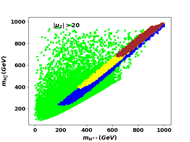
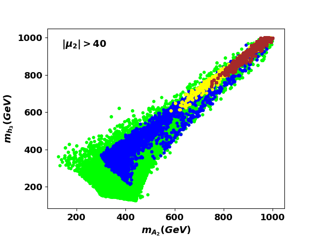
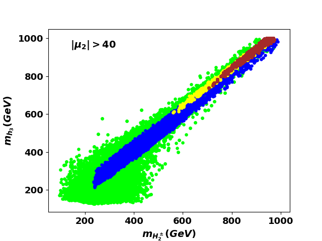
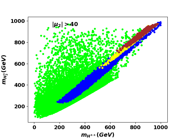
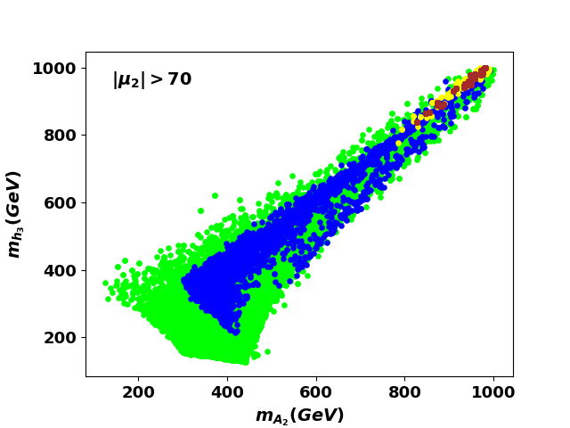
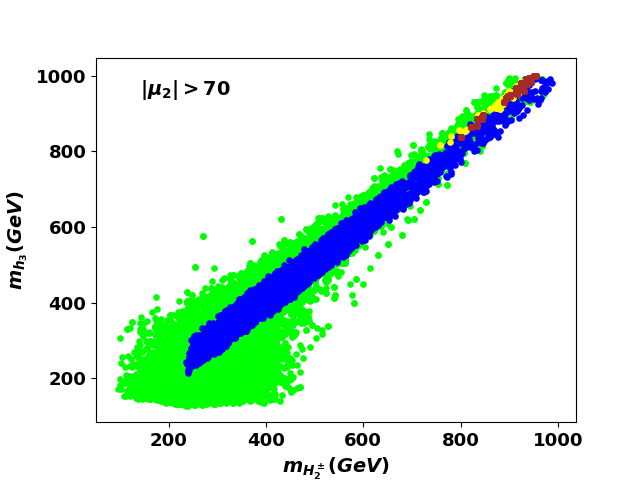
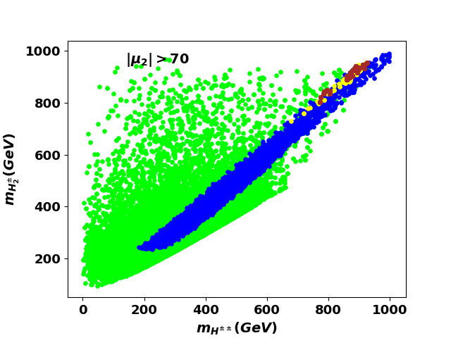
Figure 4: Allowed Higgs mass ranges in the planes $m_{\phi_{i}}$ vs $m_{\phi_{j}}$ ($\phi_{i}=$ $h_{3}$, $A_{2}$, $\phi_{i}=H^{\pm}_{2}$ and $\phi_{i}=H^{\pm\pm}$). All theoretical and experimental constraints are taken into account with color captions similar to Fig. [2].

In Fig. [1], we plot the branching ratio of $B\rightarrow X_{s}\gamma$ in the $2HDMcT$ as a function of $m_{H^{\pm}_{1}}$. $\tan\beta$ is respectively fixed to $1$ (left panel), $2$ (center panel) and $15$ (right panel) with the mass difference $\Delta M_{H^{\pm}}=m_{H^{\pm}_{2}}-m_{H^{\pm}_{1}}=20,\;50,\;and\;100$ GeV. We also used different values of the mixing angle $\theta_{3}^{\pm}$ ranging from $0.05$ corresponding to a mostly triplet $H_{2}^{\pm}(H_{1}^{\pm})$, to $\pi/4$ for a nearly equal contributions from doublets and triplet scalars to the charged Higgs bosons. For a comparative analysis, $2HDM$ prediction is also illustrated in black color. First, we see that the difference between the predictions in $2HDM$ and $2HDMcT$ becomes slightly larger as the mass difference $\Delta M_{H^{\pm}}$ or the $\theta_{3}^{\pm}$ increase. Besides, Fig. [1] uncovers two main features:

• The Higgs mass range $H_{1}^{\pm}$ satisfying the $B\rightarrow X_{s}\gamma$ constraint is almost insensitive to $\tan\beta$.

• The excluded range of the $m_{H^{\pm}_{1}}$ by $B\rightarrow X_{s}\gamma$ reduces when $\Delta M_{H^{\pm}}$ gets large.

VI ANALYSIS: IMPLICATIONS FOR THE PHYSICAL SCALAR MASSES

In this section, we focus on identifying viable regions of parameter space that satisfy all previously derived theoretical and experimental constraints. We pay special attention to the impact of three Veltman conditions $VC$’s as the experimental constraints arising from the $B\to X_{s}\gamma$ decay. Throughout the paper, $h_{1}$ is identified as the SM Higgs-like particle observed at the LHC with $m_{h_{1}}=125\;GeV$.
The input parameters, subject to the various constraints mentioned above, which we will use in the subsequent analysis, are summarized as follows:

$$\begin{matrix}m_{h_{1}}=125\,\,\text{GeV},\,\,m_{h_{1}}\leq m_{h_{2}}\leq m_{h_{3}}\leq 1\,\text{TeV},\,\,\\ 80\,\text{GeV}\leq m_{H^{\pm\pm}}\leq 1\,\text{TeV},\,\,\frac{-\pi}{2}\leq\alpha_{1}\leq\frac{\pi}{2},\,\,-0.1\leq\alpha_{2,3}\leq 0.1\\ 0.5\leq\tan\beta\leq 30,\,\,-1\leq\mu_{1}\leq 1,\,\,0\leq v_{t}\leq 1\,\text{GeV},\,\,\,\lambda_{1}\approx 0.15\\ ,\,\,\lambda_{3}\approx 1.6,\,\,\lambda_{4}\approx 1.6,\,\,-8\pi\leq\lambda_{6,7}\leq 8\pi,\,\,-8\pi\leq\lambda_{8}\leq 8\pi,\,\,-8\pi\leq\lambda_{9}\leq 8\pi\end{matrix}$$ (45)

Fo commodity purpose, we also classify the theoretical and experimental constraints into three sets :

• First set, $C_{1}$, includes the unitarity, perturbativity, vacuum stability and experimental Higgs boson exclusion limits .

• $C_{2}$, contains all constraints in $C_{1}$ in addition to the electroweak precision observables and the modified Veltman conditions.

• $C_{3}$ includes $C_{2}$ augmented by $B\to X_{s}\gamma$ constraint at 95$\%$ C.L.

We present in Fig. [2] the allowed regions in $\left(\lambda_{6}\,;\,\lambda_{8}\right)$, $\left(\lambda_{7}\,;\,\lambda_{9}\right)$ and $\left(\bar{\lambda}_{8}\,;\,\bar{\lambda}_{9}\right)$ excluded by various theoretical constraints and experimental measurements. We can see that the allowed regions of these parameter spaces undergo drastic reductions as more constraints are imposed. More specifically, they are sizably shrunk to limited yellow areas when naturalness is invoked. As a result, the potential parameters are allowed to vary within reduced intervals as shown in Table 1.

Table 1: The allowed regions of potential parameters from $C_{2}$ constraints.

parameters	intervals
$\lambda_{6}$	$[0,\;1.46]$
$\lambda_{7}$	$[0,\;1.49]$
$\lambda_{8}$	$[-1.19,\;1.57]$
$\lambda_{9}$	$[-1.34,\;1.57]$
$\bar{\lambda}_{8}$	$[-0.41,\;0.96]$
$\bar{\lambda}_{9}$	$[-0.9,\;0.86]$

Also we can observe that the parameters $\lambda_{i}$ ($i=6,7,8\,\,and\,\,9$) and $\bar{\lambda}_{8,9}$ are fully insensitive to the constraints from measurements $\bar{B}\to X_{s}\gamma$ decay rate.

As for the $\mu_{2}$ and $\mu_{3}$ parameters plotted in the left panel of Fig. [3], we see that they are more responsive to the naturalness induced conditions, particularly $T_{t}$, than to the other theoretical constraints. As a result, our analysis shows that the allowed region of $\mu_{2}$ parameter space undergoes a drastic reduction $\mu_{2}\in[-83,\;82]$, whereas $\mu_{3}$ lies within the allowed interval $\mu_{3}\in[-1230,\;1698]$. The right panel of Fig. [3] illustrates the scatter plot in $\tan\beta$ and $sgn(C_{V}^{h_{1}})\sin(\alpha_{1}-\pi/2)$ for $\Delta\chi^{2}<5.99$. When naturalness is switched off, the corresponding generated samples are shown in blue at $2\sigma$ whereas the yellow dots signal inclusion of the Veltman conditions. This graph indicates that only $\tan\beta>13$ and $\alpha_{1}\in[-1.57;-1.51]U[1.51;1.57]$ are compatible with all constraints. At this stage, it is worth noticing that the left branch with $\sin(\alpha_{1}-\frac{\pi}{2})<0$ corresponds to the SM-alignment limit, where the couplings of CP even scalars to gauge bosons are assumed to mimic the SM Higgs coupling. The right branch with $\sin(\alpha_{1}-\frac{\pi}{2})>0$ represents the wrong sign Yukaya coupling limit. If, additionally, constraints from the measurements of the $\bar{B}\to X_{s}\gamma$ decay rate at $95\%$ C.L. intervenes, then only $\alpha_{1}$ positive survives.

Fig. [4] displays the allowed region in the $(m_{A_{2}}\;,\;m_{h_{3}})$, $(m_{H^{\pm}_{2}}\;,\;m_{h_{3}})$ and $(m_{H^{\pm\pm}}\;,\;m_{H^{\pm}_{2}})$ for three ranges of $|\mu_{2}|>20,$ $40$ and $70$. Firstly, we notice a significant correlation between the mass of the Higgs boson $h_{3}$ and the mass of the Higgs boson $A_{2}$. This correlation arises from the assumptions we utilized to calculate the oblique parameters. Secondly, we find that the relevant parameter regions obeying $C_{2}$ constraints are confined within the yellow areas. The latter extents are proportional to the choice of $\mu_{2}$ range: When $\mu_{2}$ values are in the vicinity of zero, the masses are almost insensitive to the naturalness (set $C_{3}$). However, if $\mu_{2}$ moves away from zero, the mass ranges are clearly reduced by $VC$ conditions. The brown color represents the surviving parameter regions to all constraints. Therefore as summarized by Table 2, we can conclude that the naturalness has a substantial impact on both the lower bounds of the heavy Higgs spectra and on the upper bounds of the light Higgs bosons masses. It is worth noticing that this general trend persists even if the mass scale, initially fixed to $1$ TeV, is shifted up. More specifically, we see that the lower bounds of the Higgs mass ranges are insensitive to the increase in scale, while the upper bounds are evidently pushed up to higher values, as expected.

Table 2: Higgs masses allowed intervals from various constraints, including the modified Veltman conditions for $\delta T=3.5$ GeV

$m_{\phi}$	Unitarity	Unitarity+BFB	$\;C_{1}$ constraints
$m_{h_{2}}$	$[126\,;\,990]$	$[126\,;\,910]$	$[137\,;\,905]$
$m_{h_{3}}$	$[126\,;\,1000]$	$[127\,;\,1000]$	$[266\,;\,999]$
$m_{A_{1}}$	$[80\,;\,992]$	[80 ; 930]	$[128\,;\,903]$
$m_{A_{2}}$	$[126\,;\,1000]$	$[127\,;\,1000]$	$[266\,;\,999]$
$m_{H^{\pm}_{1}}$	$[80\,;\,991]$	$[80\,;\,933]$	$[218\,;\,913]$
$m_{H^{\pm}_{2}}$	$[88\,;\,998]$	$[95\,;\,991]$	$[276\,;\,982]$
$m_{H^{\pm\pm}}$	$[80\,;\,1000]$	$[80\,;\,1000]$	$[235\,;\,997]$

$m_{\phi}$	$C_{2}$ constraints
	$|\mu_{2}|>20$ GeV	$|\mu_{2}|>40$ GeV	$|\mu_{2}|>70$ GeV
$m_{h_{2}}$	$[145\,;\,930]$	$[160\,;\,880]$	$[167\,;\,795]$
$m_{h_{3}}$	$[415\,;\,999]$	$[607\,;\,999]$	$[778\,;\,999]$
$m_{A_{1}}$	$[145\,;\,950]$	$[170\,;\,920]$	$[236\,;\,840]$
$m_{A_{2}}$	$[415\,;\,999]$	$[607\,;\,999]$	$[778\,;\,999]$
$m_{H^{\pm}_{1}}$	$[222\,;\,980]$	$[266\,;\,918]$	$[328\,;\,840]$
$m_{H^{\pm}_{2}}$	$[391\,;\,987]$	$[560\,;\,976]$	$[728\,;\,956]$
$m_{H^{\pm\pm}}$	$[335\,;\,995]$	$[515\,;\,976]$	$[679\,;\,928]$

$m_{\phi}$	$C_{3}$ constraints
	$|\mu_{2}|>20$ GeV	$|\mu_{2}|>40$ GeV	$|\mu_{2}|>70$ GeV
$m_{h_{2}}$	$[487\,;\,927]$	$[490\,;\,879]$	$[511\,;\,790]$
$m_{h_{3}}$	$[719\,;\,999]$	$[737\,;\,999]$	$[837\,;\,982]$
$m_{A_{1}}$	$[576\,;\,947]$	$[576\,;\,910]$	$[596\,;\,838]$
$m_{A_{2}}$	$[719\,;\,999]$	$[737\,;\,999]$	$[837\,;\,982]$
$m_{H^{\pm}_{1}}$	$[592\,;\,946]$	$[599\,;\,915]$	$[623\,;\,839]$
$m_{H^{\pm}_{2}}$	$[683\,;\,985]$	$[706\,;\,973]$	$[801\,;\,954]$
$m_{H^{\pm\pm}}$	$[632\,;\,990]$	$[654\,;\,973]$	$[772\,;\,925]$

VII CONCLUSION

In this paper, we have extended the work Ouazghour:2018mld by investigating naturalness problem and B physics constraints within the context of two Higgs doublets type II seesaw model ($2HDMcT$). We have derived the modified Vetman conditions in $2HDMcT$ and showed that the naturalness problem might be avoided within the model parameter space at the electroweak scale. Next, we have calculated the branching ratio of $\bar{B}\to X_{s}\gamma$ radiative decay at the $NLO$ and showed that $\bar{B}\to X_{s}\gamma$ constraint can only be accommodated provided that the parameter $\alpha_{1}$ is always positive and the Higgs mass hierarchy $m_{h_{3}}>m_{H_{2}^{\pm}}>m_{H^{\pm\pm}}$ satisfied. Th main outcome of our current analysis is to show how these additional new constraints, $VC$ and $\bar{B}\to X_{s}\gamma$, induce significant delimitations of the $2HDMcT$ parameter space with respect to the results reported in Ouazghour:2018mld . As a consequence, it is demonstrated that the Higgs spectrum is utterly reshaped with the heavy Higgs $h_{3}$, $A_{2}$, $H_{2}^{\pm}$ and $H^{\pm\pm}$ masses significantly affected. Three benchmark scenarios corresponding to $\mu_{2}>20,40,70$ GeV have been explored. For $\mu_{2}>40$ GeV, we found that the lower mass limits of nonstandard Higgs bosons ($h_{2}$, $h_{3}$, $A_{1}$, $A_{2}$, $H_{1}^{\pm}$, $H_{2}^{\pm}$, $H^{\pm\pm}$) are pushed up to higher values ranging from $490$ to $750$ GeV.

References

- (1) B. A. Ouazghour, A. Arhrib, R. Benbrik, M. Chabab, and L. Rahili, Theory and phenomenology of a two-Higgs-doublet type-II seesaw model at the LHC run 2, Phys. Rev. D 100 (2019), no. 3 035031, [arXiv:1812.07719].
- (2) ATLAS Collaboration, G. Aad et al., Observation of a new particle in the search for the Standard Model Higgs boson with the ATLAS detector at the LHC, Phys. Lett. B 716 (2012) 1–29, [arXiv:1207.7214].
- (3) G. Aad et al., Atlas collaboration, Phys. Lett. B 726 (2013) 120.
- (4) CMS Collaboration, S. Chatrchyan et al., Observation of a New Boson at a Mass of 125 GeV with the CMS Experiment at the LHC, Phys. Lett. B 716 (2012) 30–61, [arXiv:1207.7235].
- (5) CMS Collaboration, S. Chatrchyan et al., Observation of a New Boson with Mass Near 125 GeV in Collisions at = 7 and 8 TeV, JHEP 06 (2013) 081, [arXiv:1303.4571].
- (6) J. F. Gunion, The Higgs hunter’s guide. CRC Press, 2018.
- (7) ATLAS, CMS Collaboration, G. Aad et al., Combined Measurement of the Higgs Boson Mass in Collisions at and 8 TeV with the ATLAS and CMS Experiments, Phys. Rev. Lett. 114 (2015) 191803, [arXiv:1503.07589].
- (8) G. B. Pivovarov and V. T. Kim, On Naturalness of Scalar Fields and Standard Model, Phys. Rev. D 78 (2008) 016001, [arXiv:0712.0402].
- (9) M. Chabab, M. C. Peyranère, and L. Rahili, Naturalness in a type II seesaw model and implications for physical scalars, Phys. Rev. D 93 (2016), no. 11 115021, [arXiv:1512.07280].
- (10) M. Chabab, M. C. Peyranère, and L. Rahili, Probing the Higgs sector of Higgs Triplet Model at LHC, Eur. Phys. J. C 78 (2018), no. 10 873, [arXiv:1805.00286].
- (11) B. Grzadkowski and J. Wudka, Naive solution of the little hierarchy problem and its physical consequences, Acta Phys. Polon. B 40 (2009) 3007–3014, [arXiv:0910.4829].
- (12) C. N. Karahan and B. Korutlu, Effects of a Real Singlet Scalar on Veltman Condition, Phys. Lett. B 732 (2014) 320–324, [arXiv:1404.0175].
- (13) A. Das, S. Mandal, and S. Shil, Testing electroweak scale seesaw models at e- and colliders, Phys. Rev. D 108 (2023), no. 1 015022, [arXiv:2304.06298].
- (14) N. Darvishi and M. Krawczyk, Implication of Quadratic Divergences Cancellation in the Two Higgs Doublet Model, Nucl. Phys. B 926 (2018) 167–178, [arXiv:1709.07219].
- (15) B. Ait-Ouazghour and M. Chabab, The Higgs potential in 2HDM extended with a real triplet scalar: A roadmap, Int. J. Mod. Phys. A 36 (2021), no. 19 2150131, [arXiv:2006.12233].
- (16) M. J. Ramsey-Musolf, The electroweak phase transition: a collider target, JHEP 09 (2020) 179, [arXiv:1912.07189].
- (17) C.-H. Chen and T. Nomura, Inert Dark Matter in Type-II Seesaw, JHEP 09 (2014) 120, [arXiv:1404.2996].
- (18) C.-H. Chen and T. Nomura, Two-Higgs-Doublet Type-II Seesaw Model, Phys. Rev. D 90 (2014), no. 7 075008, [arXiv:1406.6814].
- (19) P. Bechtle, O. Brein, S. Heinemeyer, G. Weiglein, and K. E. Williams, Higgsbounds: confronting arbitrary higgs sectors with exclusion bounds from lep and the tevatron, Computer Physics Communications 181 (2010), no. 1 138–167.
- (20) P. Bechtle, O. Brein, S. Heinemeyer, G. Weiglein, and K. E. Williams, Higgsbounds 2.0. 0: confronting neutral and charged higgs sector predictions with exclusion bounds from lep and the tevatron, Computer Physics Communications 182 (2011), no. 12 2605–2631.
- (21) P. Bechtle, O. Brein, S. Heinemeyer, O. Stål, T. Stefaniak, G. Weiglein, and K. E. Williams, Higgsbounds-4: improved tests of extended higgs sectors against exclusion bounds from lep, the tevatron and the lhc, The European Physical Journal C 74 (2014) 1–32.
- (22) P. Bechtle, D. Dercks, S. Heinemeyer, T. Klingl, T. Stefaniak, G. Weiglein, and J. Wittbrodt, Higgsbounds-5: testing higgs sectors in the lhc 13 tev era, The European Physical Journal C 80 (2020) 1–24.
- (23) H. Bahl, V. M. Lozano, T. Stefaniak, and J. Wittbrodt, Testing exotic scalars with higgsbounds, The European Physical Journal C 82 (2022), no. 7 584.
- (24) P. Bechtle, S. Heinemeyer, O. Stål, T. Stefaniak, and G. Weiglein, Higgssignals: Confronting arbitrary higgs sectors with measurements at the tevatron and the lhc, The European Physical Journal C 74 (2014) 1–40.
- (25) P. Bechtle, S. Heinemeyer, T. Klingl, T. Stefaniak, G. Weiglein, and J. Wittbrodt, Higgssignals-2: Probing new physics with precision higgs measurements in the lhc 13 tev era, The European Physical Journal C 81 (2021) 1–36.
- (26) L. Lavoura and L.-F. Li, Making the small oblique parameters large, Phys. Rev. D 49 (1994) 1409–1416, [hep-ph/9309262].
- (27) W. Grimus, L. Lavoura, O. M. Ogreid, and P. Osland, A Precision constraint on multi-Higgs-doublet models, J. Phys. G 35 (2008) 075001, [arXiv:0711.4022].
- (28) W. Grimus, L. Lavoura, O. M. Ogreid, and P. Osland, The Oblique parameters in multi-Higgs-doublet models, Nucl. Phys. B 801 (2008) 81–96, [arXiv:0802.4353].
- (29) W. Grimus, L. Lavoura, O. Ogreid, and P. Osland, The oblique parameters in multi-higgs-doublet models 2008, Nucl. Phys. B 801 no. 81 0802–4353.
- (30) Particle Data Group Collaboration, P. A. Zyla et al., Review of Particle Physics, PTEP 2020 (2020), no. 8 083C01.
- (31) M. J. G. Veltman, The Infrared - Ultraviolet Connection, Acta Phys. Polon. B 12 (1981) 437.
- (32) W. Siegel, Supersymmetric dimensional regularization via dimensional reduction, Physics Letters B 84 (1979), no. 2 193–196.
- (33) M. Einhorn and D. Jones, Effective potential and quadratic divergences, Physical Review D 46 (1992), no. 11 5206.
- (34) M. Al-Sarhi, I. Jack, and D. Jones, Quadratic divergences in gauge theories, Zeitschrift für Physik C Particles and Fields 55 (1992) 283–287.
- (35) C. Newton and T. T. Wu, Mass relations in the two Higgs doublet model from the absence of quadratic divergences, Z. Phys. C 62 (1994) 253–264.
- (36) C. Newton, P. Osland, and T. T. Wu, Can the higgs boson be detected at the fermilab tevatron collider?, Zeitschrift für Physik C Particles and Fields 61 (1994) 421–423.
- (37) M. S. Al-Sarhi, D. R. T. Jones, and I. Jack, Quadratic divergences and dimensional regularization in two-dimensions and four-dimensions, Nucl. Phys. B 345 (1990) 431–444.
- (38) M. B. Einhorn and D. R. T. Jones, The Effective potential and quadratic divergences, Phys. Rev. D 46 (1992) 5206–5208.
- (39) B. Grzadkowski and J. Wudka, Pragmatic approach to the little hierarchy problem: the case for Dark Matter and neutrino physics, Phys. Rev. Lett. 103 (2009) 091802, [arXiv:0902.0628].
- (40) B. Grzadkowski and P. Osland, Natural Two-Higgs-Doublet Model, Fortsch. Phys. 59 (2011) 1041–1045, [arXiv:1012.0703].
- (41) A. Drozd, B. Grzadkowski, and J. Wudka, Multi-scalar-singlet extension of the standard model—the case for dark matter and an invisible higgs boson, Journal of High Energy Physics 2012 (2012), no. 4 1–27.
- (42) F. Bazzocchi and M. Fabbrichesi, Little hierarchy problem for new physics just beyond the LHC, Phys. Rev. D 87 (2013), no. 3 036001, [arXiv:1212.5065].
- (43) I. Masina and M. Quiros, On the Veltman Condition, the Hierarchy Problem and High-Scale Supersymmetry, Phys. Rev. D 88 (2013) 093003, [arXiv:1308.1242].
- (44) I. Chakraborty and A. Kundu, Two-Higgs doublet models confront the naturalness problem, Phys. Rev. D 90 (2014), no. 11 115017, [arXiv:1404.3038].
- (45) A. Biswas and A. Lahiri, Masses of physical scalars in two Higgs doublet models, Phys. Rev. D 91 (2015), no. 11 115012, [arXiv:1412.6187].
- (46) D. Chowdhury and O. Eberhardt, Global fits of the two-loop renormalized two-higgs-doublet model with soft z 2 breaking, Journal of High Energy Physics 2015 (2015), no. 11 1–36.
- (47) F. M. Borzumati and C. Greub, Two higgs doublet model predictions for in nlo qcd, Physical Review D 58 (1998), no. 7 074004.
- (48) Belle Collaboration, T. Saito et al., Measurement of the Branching Fraction with a Sum of Exclusive Decays, Phys. Rev. D 91 (2015), no. 5 052004, [arXiv:1411.7198].
- (49) BaBar Collaboration, B. Aubert et al., Measurement of the branching fraction and photon energy spectrum using the recoil method, Phys. Rev. D 77 (2008) 051103, [arXiv:0711.4889].
- (50) BaBar Collaboration, J. P. Lees et al., Precision Measurement of the Photon Energy Spectrum, Branching Fraction, and Direct CP Asymmetry , Phys. Rev. Lett. 109 (2012) 191801, [arXiv:1207.2690].
- (51) BaBar Collaboration, J. P. Lees et al., Exclusive Measurements of Transition Rate and Photon Energy Spectrum, Phys. Rev. D 86 (2012) 052012, [arXiv:1207.2520].
- (52) CLEO Collaboration, S. Chen et al., Branching fraction and photon energy spectrum for , Phys. Rev. Lett. 87 (2001) 251807, [hep-ex/0108032].
- (53) HFLAV Collaboration, Y. S. Amhis et al., Averages of -hadron, -hadron, and -lepton properties as of 2021, Phys. Rev. D 107 (2023) 052008, [arXiv:2206.07501].