Preparing highly entangled states of nanodiamond rotation and NV center spin

Abstract

A nanodiamond with an embedded nitrogen-vacancy (NV) center is one of the experimental systems that can be coherently manipulated within current technologies. Entanglement between NV center electron spin and mechanical rotation of the nanodiamond plays a fundamental role in building a quantum network connecting these microscopic and mesoscopic degrees of motions. Here we present a protocol to asymptotically prepare a highly entangled state of the total quantum angular momentum and electron spin by adiabatically boosting the external magnetic field.

I Introduction

Experimental accomplishments of cooling and controlling of microscale particles make it possible to exploit macroscopic quantum systems. The nitrogen-vacancy (NV) centers in diamond have shown impressive applications in quantum sensing, and in quantum information processing and communications [1, 2, 3]. Nanodiamonds with NV centers trapped in vacuum can be cooled into their centre-of-mass ground state [4, 5, 6] and be used to generate spatial quantum superpositions [7, 8, 9, 10]. While in recent years the rotation control of nanoparticle with ultra-high precision [11, 12, 13, 14, 15] opens the path to observing and testing rotational superpositions [16, 17, 18, 19, 20, 21]. In a view of quantum information, the coupling of NV center spin and the nanodiamond rotation contains entanglement resource [22]. Study of the entanglement property of the spin-rotation coupled system may have potential use in quantum sensing and in quantum network.

In this paper, we simplify the system to an ideal model by considering the nanodiamond only in an external magnetic field. The nanodiamond is treated as a rigid body and its rotation can be described by angular momentum theory in quantum physics [23, 24, 25]. We show that by boosting the external magnetic field strength a highly entangled state of NV center spin and total angular momentum can be realized asymptotically.

II Our Model and problem

As shown in section II, we consider a nanodiamond, modeled as a symmetric top whose shape is a tetrahedron. The nanodiamond hosts a single negatively charged nitrogen-vacancy center (NV^-) with the spin angular momentum $\hat{{\bf\it S}}$ whose quantization axis aligned with the nanodiamond symmetric axis. The ground state structure of the spin-1 NV^- center is shown in section II. We suppose the nanodiamond’s mechanic rotation is free. In a magnetic field $\vec{B}=B\vec{e}_{3}$ along the $\vec{e}_{3}$-direction of the space-fixed frame with axes $\{\vec{e}_{1},\vec{e}_{2},\vec{e}_{3}\}$, the spin of the NV^- center and the rotation of the diamond are coupled, and the system is described by the Hamiltonian

$$H=H_{0}+V$$ (1)

with

$$H_{0} =\frac{D}{\hbar}\hat{S}^{\prime 2}_{3}+\frac{1}{2}\frac{\hat{{\bf\it L}}^{2}}{I_{1}}+\frac{1}{2}\biggl{(}\frac{1}{I_{3}}-\frac{1}{I_{1}}\biggr{)}{\hat{L}_{3}^{\prime 2}},$$ (2)

$$V =\frac{g\mu_{B}}{\hbar}B\sum_{i=1}^{3}\hat{S}_{i}^{\prime}\hat{\vec{e}}_{i}^{\prime}\dotproduct\vec{e}_{3}$$ (3)

where $\{\hat{\vec{e}}_{1}^{\prime},\hat{\vec{e}}_{2}^{\prime},\hat{\vec{e}}_{3}^{\prime}\}$ are the principle axes of the nanodiamond and form the body-fixed frame, which are dynamic operators related with rotations. $\hat{{\bf\it L}}$ is the rotation angular momentum operator. $\{I_{1},I_{2},I_{3}\}$ are the principle inertia moments with $I_{1}=I_{2}$ for a symmetric top. $\hat{S}^{\prime}_{i}$ ($\hat{L}^{\prime}_{i}$) is the projection component operator of $\hat{{\bf\it S}}$ ($\hat{{\bf\it L}}$) along the body-fixed $\vec{e}_{i}^{\prime}$-axis. $\mu_{B}$ is the Bohr magneton. The zero-field-splitting of the spin triplet ground state $D\simeq(2\pi)$2.87\text{\,}\mathrm{GHz}$$, and the isotropic NV^- center electron g-factor $g\simeq 2.0028$ [26].

When we write the Hamiltonian in body frame, we should be careful about the commutation relations of the operators [27]. Notice that the spin compenents $\hat{S}^{\prime}_{i}$ are not commuting with the angular momentum compenents $\hat{L}^{\prime}_{i}$ since $\hat{S}^{\prime}_{i}\equiv\hat{\vec{e}}^{\prime}_{i}\dotproduct\hat{{\bf\it S}}$, we introduce the total angular momentum operator $\hat{{\bf\it J}}=\hat{{\bf\it L}}+\hat{{\bf\it S}}$ whose projection compenents on body frame axes are commuting with the spin compenents, i.e. $\commutator*{\hat{J}^{\prime}_{i}}{\hat{S}^{\prime}_{j}}=0$.

The problem we aim to solve is to investigate how the entanglement between nanodiamond’s total angular momentum and its spin in the thermal equilibrium state varies as a function of magnetic field and temperature, where the thermal state is

$$\rho(B,T)=\frac{e^{-\beta H}}{\mathrm{Tr}e^{-\beta H}},$$ (4)

where $\beta=\frac{1}{k_{B}T}$ with $k_{B}$ being the Boltzmann constant. As the temperature limits to zero, the thermal equilibrium state becomes the ground state:

$$\lim_{T\rightarrow 0}\rho(B,T)=|G(B)\rangle\langle G(B)|.$$ (5)

Figure 1.: The fine and Zeeman structures of the NV^- center ground state. The structure levels are denoted by their spin-orbit symmetry and spin projections $m\in\{0,\pm 1\}$.

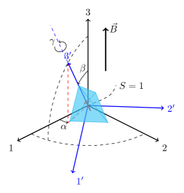
Figure 2.: Sketch of the nanodiamond with an embedded NV^- center in external magnetic field $B$. $\{\alpha,\beta,\gamma\}$ are Euler angles between the space-fixed frame and the body-fixed frame.

III Eigen problem of the Hamiltonian

Before exploring the entanglement between the total angular momentum and the spin in the thermal equilibrium state $\rho(B,T)$ or in the ground state $|G(B)\rangle$, it is necessary for us to solve the eigen problem of the Hamiltonian (1). Rewrite the Hamiltonian by inserting $\hat{{\bf\it L}}=\hat{{\bf\it J}}-\hat{{\bf\it S}}=\hat{{\bf\it J}}+\hat{{\bf\it K}}$,

$$H_{0} =\frac{D}{\hbar}\hat{K}^{\prime 2}_{3}+\frac{1}{2I_{1}}(\hat{\mathbf{J}}^{2}+2\hat{J}^{\prime}_{3}\hat{K}^{\prime}_{3}+\hat{J}^{\prime}_{+}\hat{K}^{\prime}_{-}+\hat{J}^{\prime}_{-}\hat{K}^{\prime}_{+})$$

$$+\pqty{\frac{1}{I_{3}}-\frac{1}{I_{1}}}\frac{(\hat{J}^{\prime}_{3}+\hat{K}^{\prime}_{3})^{2}}{2},$$

$$V =-\frac{g\mu_{B}}{\hbar}\hat{\mathbf{K}}\dotproduct\mathbf{B},$$ (6)

where we have let $\hat{{\bf\it K}}\equiv-\hat{{\bf\it S}}$ with $K\equiv S\equiv 1$ in our problem and dropped $\hat{\mathbf{S}}^{2}=S(S+1)$. And the ladder operators are

$$\hat{J}^{\prime}_{\pm} =\hat{J}^{\prime}_{1}\mp\mathrm{i}\hat{J}^{\prime}_{2},$$ (7)

$$\hat{K}^{\prime}_{\pm} =\hat{K}^{\prime}_{1}\mp\mathrm{i}\hat{K}^{\prime}_{2}.$$ (8)

III.1 Basis states based on $H_{0}$

First we study the degree of the nanodiamond rotation. Because $\hat{\bm{L}}$ is an angular momentum operator, it obeys the following commutation relations

$$\commutator{\hat{L}_{i}}{\hat{L}_{j}} =i\hbar\epsilon_{ijk}\hat{L}_{k},$$ (9)

$$\commutator{\hat{L}_{i}}{\hat{\vec{e}}_{l}^{\prime}\dotproduct\vec{e}_{j}} =i\hbar\epsilon_{ijk}\hat{\vec{e}}_{l}^{\prime}\dotproduct\vec{e}_{k},$$ (10)

where $i,j,k\in\{1,2,3\}$ and $l\in\{1,2,3\}$, and $\epsilon_{ijk}$ is antisymmetric tensor with $\epsilon_{123}=1$. Note that $\hat{L}^{\prime}_{i}\equiv\hat{\vec{e}}^{\prime}_{i}\dotproduct\hat{{\bf\it L}}$. Then a direct calculation gives

$$\commutator{\hat{L}^{\prime}_{i}}{\hat{L}^{\prime}_{j}}=-i\hbar\epsilon_{ijk}\hat{L}^{\prime}_{k},$$ (11)

where $i,j,k\in\{1,2,3\}$. Compared Eq. 11 with Eq. 9, it is interesting to observe that a negative sign appears in the commutation relations of the angular momentum in the body-fixed frame. With the relations $\hat{S}^{\prime}_{i}\equiv\hat{\vec{e}}^{\prime}_{i}\dotproduct\hat{{\bf\it S}}=\sum_{j=1}^{3}\hat{\vec{e}}^{\prime}_{i}\dotproduct\vec{e}_{j}\hat{S}_{j}$, one can give the following commutation relations:

$$\commutator{\hat{J}^{\prime}_{i}}{\hat{J}^{\prime}_{j}} =-\mathrm{i}\epsilon_{ijk}\hat{J}^{\prime}_{k},$$ (12)

$$\commutator{\hat{K}^{\prime}_{i}}{\hat{K}^{\prime}_{j}} =-\mathrm{i}\epsilon_{ijk}\hat{K}^{\prime}_{k},$$ (13)

$$\commutator{\hat{J}^{\prime}_{3}}{\hat{K}^{\prime}_{3}} =0,$$ (14)

$$\commutator{\hat{J}_{3}}{\hat{K}^{\prime}_{3}} =0.$$ (15)

The total angular momentum

$$\hat{{\bf\it J}}^{2}=\sum_{i}\hat{J}_{i}^{2}=\sum_{i}\hat{J}_{i}^{{}^{\prime}2},$$ (16)

which builds a relation between the angular momentum operators in these two frames. Then we find that

$$\commutator{\hat{{\bf\it J}}^{2}}{\hat{J}_{3}} =0,$$ (17)

$$\commutator{\hat{{\bf\it J}}^{2}}{\hat{J}^{\prime}_{3}} =0,$$ (18)

$$\commutator{\hat{J}_{3}}{\hat{J}^{\prime}_{3}} =0,$$ (19)

which implies that $\{\hat{{\bf\it J}}^{2},\hat{J}_{3},\hat{J}^{\prime}_{3},\hat{{\bf\it K}}^{2},\hat{K}^{\prime}_{3}\}$ forms a complete set of commuting observables for the degree of freedom of the system. They have the common eigenstates

$$\ket{\varphi}=\ket{Jm_{J}k_{J},Kk_{K}}.$$ (20)

such that

$$\hat{{\bf\it J}}^{2}\ket{\varphi} =J(J+1)\ket{\varphi},$$ (21)

$$\hat{J}_{3}\ket{\varphi} =m_{J}\ket{\varphi},$$ (22)

$$\hat{J}^{\prime}_{3}\ket{\varphi} =k_{J}\ket{\varphi},$$ (23)

$$\hat{{\bf\it K}}^{2}\ket{\varphi} =K(K+1)\ket{\varphi},$$ (24)

$$\hat{K}^{\prime}_{3}\ket{\varphi} =k_{K}\ket{\varphi},$$ (25)

where $J\in\{0,1,\cdots\}$, $m_{J},k_{J}\in\{-J,-J+1,\cdots,J-1,J\}$, $k_{K}\in\{-1,0,1\}$, and these common eigenstates form a set of base vectors of the full Hilbert space. Then the matrix elements of the ladder operators $\hat{J}^{\prime}_{\pm}$ and $\hat{K}^{\prime}_{\pm}$ are given by the following relations,

$$\hat{J}^{\prime}_{\pm}\ket{Jm_{J}k_{J},Kk_{K}}$$

$$=\sqrt{(J\mp k_{J})(J\pm k_{J}+1)}\ket{Jm_{J}k_{J}\pm 1,Kk_{K}},$$ (26)

$$\hat{K}^{\prime}_{\pm}\ket{Jm_{J}k_{J},Kk_{K}}$$

$$=\sqrt{(K\mp k_{K})(K\pm k_{K}+1)}\ket{Jm_{J}k_{J},Kk_{K}\pm 1}.$$ (27)

For $K=1$, it’s convenient to write out the $\hat{K}^{\prime}_{i}$ matrices

$$K^{\prime}_{1} =\frac{1}{\sqrt{2}}\begin{pmatrix}0&1&0\\ 1&0&1\\ 0&1&0\end{pmatrix},$$ (28)

$$K^{\prime}_{2} =\frac{-i}{\sqrt{2}}\begin{pmatrix}0&-1&0\\ 1&0&-1\\ 0&1&0\end{pmatrix},$$ (29)

$$K^{\prime}_{3} =\begin{pmatrix}1&0&0\\ 0&0&0\\ 0&0&-1\end{pmatrix}.$$ (30)

III.2 Analytical matrix elements in $V$

The next task is to calculate the matrix element $\bra*{J^{\prime}m_{J}^{\prime}k_{J}^{\prime},Kk_{K}^{\prime}}V\ket*{Jm_{J}k_{J},Kk_{K}}$. In other words, we need to calculate the matrix elements $\bra*{J^{\prime}m_{J}^{\prime}k_{J}^{\prime}}\hat{\vec{e}}^{\prime}_{i}\dotproduct\vec{e}_{j}\ket*{Jm_{J}k_{J}}$.

Because all the operators $\{\hat{\vec{e}}^{\prime}_{l}\dotproduct\vec{e}_{i}\}$ are commutative to each other, we can introduce their common eigenstates

$$\hat{\vec{e}}^{\prime}_{l}\dotproduct\vec{e}_{i}|\alpha\beta\gamma\rangle=\vec{e}^{\prime}_{l}\dotproduct\vec{e}_{i}|\alpha\beta\gamma\rangle,$$ (31)

where $\{\alpha,\beta,\gamma\}$ are three Euler angles (illustrated in section II). In particular

$$\hat{\vec{e}}^{\prime}_{1}\dotproduct\vec{e}_{3}|\alpha\beta\gamma\rangle =-\cos{\gamma}\sin{\beta}|\alpha\beta\gamma\rangle,$$ (32)

$$\hat{\vec{e}}^{\prime}_{2}\dotproduct\vec{e}_{3}|\alpha\beta\gamma\rangle =\sin{\gamma}\sin{\beta}|\alpha\beta\gamma\rangle,$$ (33)

$$\hat{\vec{e}}^{\prime}_{3}\dotproduct\vec{e}_{3}|\alpha\beta\gamma\rangle =\cos{\beta}|\alpha\beta\gamma\rangle.$$ (34)

Then

$$\bra{J^{\prime}m_{J}^{\prime}k_{J}^{\prime}}\hat{\vec{e}}^{\prime}_{i}\dotproduct\vec{e}_{3}\ket{Jm_{J}k_{J}}$$

$$=\int\differential\omega\vec{e}^{\prime}_{i}\dotproduct\vec{e}_{3}\innerproduct{J^{\prime}m_{J}^{\prime}k_{J}^{\prime}}{\alpha\beta\gamma}\innerproduct{\alpha\beta\gamma}{Jm_{J}k_{J}},$$ (35)

where $\mathrm{d}\omega=\sin\beta\mathrm{d}\alpha\mathrm{d}\beta\mathrm{d}\gamma$ with $\alpha,\gamma\in[0,2\pi]$ and $\beta\in[0,\pi]$. The eigenfunction $\innerproduct{\alpha\beta\gamma}{Jm_{J}k_{J}}$ can be written as

$$\innerproduct{\alpha\beta\gamma}{Jm_{J}k_{J}}=\sqrt{\frac{2J+1}{8\pi^{2}}}D_{k_{J}m_{J}}^{(J)}(\alpha,\beta,\gamma),$$ (36)

where $D_{k_{J}m_{J}}^{(J)}(\alpha,\beta,\gamma)$ is the matrix representation of Euler rotation operator $\hat{R}(\alpha,\beta,\gamma)$ in Hilbert space (more details see appendix A).

A set of spherical basis vectors in space-fixed frame can be defined as

$$\vec{\xi}_{+1} \equiv-(\vec{e}_{1}+i\vec{e}_{2})/\sqrt{2},$$ (37)

$$\vec{\xi}_{0} \equiv\vec{e}_{3},$$ (38)

$$\vec{\xi}_{-1} \equiv(\vec{e}_{1}-i\vec{e}_{2})/\sqrt{2},$$ (39)

with the orthogonality relations

$$\vec{\xi}^{*}_{\mu}\dotproduct\vec{\xi}_{\nu}=\delta_{\mu\nu},$$ (40)

where $\nu,\mu\in\{+1,0,-1\}$, and $\vec{\xi}^{\ast}_{\mu}$ is the complex conjugate of $\vec{\xi}_{\mu}$. Then we can show that $\{\vec{\xi}_{\mu}\}$ and $\{\vec{\xi}^{\prime}_{\mu}\}$ obey the transformation

$$\vec{\xi}_{\mu}=\sum_{\nu}D^{(1)}_{\nu\mu}(\alpha,\beta,\gamma)\vec{\xi}^{\prime}_{\nu}.$$ (41)

Combine Eqs. 37, 38, 39, 40 and 41, we have

$$\vec{\xi}^{\prime*}_{\mu}\dotproduct\vec{e}_{3}=\vec{\xi}^{\prime*}_{\mu}\dotproduct\vec{\xi}_{0}=D^{(1)}_{\mu 0}(\alpha,\beta,\gamma).$$ (42)

Then

$$\vec{e}^{\prime}_{1}\dotproduct\vec{e}_{3} =\pqty{-D^{(1)}_{10}(\alpha,\beta,\gamma)+D^{(1)}_{-1\;0}}/\sqrt{2},$$

$$\vec{e}^{\prime}_{2}\dotproduct\vec{e}_{3} =-i\pqty{D^{(1)}_{10}(\alpha,\beta,\gamma)+D^{(1)}_{-1\;0}}/\sqrt{2},$$

$$\vec{e}^{\prime}_{3}\dotproduct\vec{e}_{3} =D^{(1)}_{00}(\alpha,\beta,\gamma).$$ (43)

Employing the identity of the integral of three $D_{\nu\mu}^{(J)}(\alpha,\beta,\gamma)$ functions:

$$\int D_{m_{1}^{\prime}m_{1}}^{(J_{1})}(\alpha,\beta,\gamma)D_{m_{2}^{\prime}m_{2}}^{(J_{2})}(\alpha,\beta,\gamma)D_{m_{3}^{\prime}m_{3}}^{(J_{3})}(\alpha,\beta,\gamma)\frac{\differential\omega}{8\pi^{2}}$$

$$=\begin{pmatrix}J_{1}&J_{2}&J_{3}\\ m^{\prime}_{1}&m^{\prime}_{2}&m^{\prime}_{3}\end{pmatrix}\begin{pmatrix}J_{1}&J_{2}&J_{3}\\ m_{1}&m_{2}&m_{3}\end{pmatrix},$$ (44)

and their complex conjugate relations

$$D_{\nu\mu}^{(J)*}(\alpha,\beta,\gamma)=(-1)^{\nu-\mu}D_{-\nu,-\mu}^{(J)}(\alpha,\beta,\gamma),$$ (45)

we arrive at an analytical result of the integral

$$\bra{J^{\prime}m_{J}^{\prime}k_{J}^{\prime}}D_{\mu 0}^{(1)}(\alpha,\beta,\gamma)\ket{Jm_{J}k_{J}}$$

$$=\int\frac{\differential\omega}{8\pi^{2}}\sqrt{(2J^{\prime}+1)(2J+1)}$$

$$\quad\times D_{k_{J}^{\prime}m_{J}^{\prime}}^{(J^{\prime})*}(\alpha,\beta,\gamma)D_{\mu 0}^{(1)}(\alpha,\beta,\gamma)D_{k_{J}m_{J}}^{(J)}(\alpha,\beta,\gamma)$$

$$=(-1)^{k_{J}^{\prime}-m_{J}^{\prime}}\sqrt{(2J^{\prime}+1)(2J+1)}$$

$$\quad\times\begin{pmatrix}J^{\prime}&1&J\\ -k_{J}^{\prime}&\mu&k_{J}\end{pmatrix}\begin{pmatrix}J^{\prime}&1&J\\ -m_{J}^{\prime}&0&m_{J}\end{pmatrix},$$ (46)

where the rhs of section III.2 are two $3J$-symbols. Inserting section III.2 and section III.2 into section III.2, we get the matrix element $\bra{J^{\prime}m_{J}^{\prime}k_{J}^{\prime}}\hat{\vec{e}}^{\prime}_{i}\dotproduct\vec{e}_{3}\ket{Jm_{J}k_{J}}$. Combine with $\hat{K}^{\prime}_{i}$, we get the matrix element $\bra*{J^{\prime}m_{J}^{\prime}k_{J}^{\prime},Kk_{K}^{\prime}}V\ket*{Jm_{J}k_{J},Kk_{K}}$.

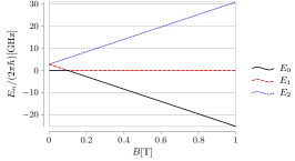
(a)

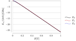
(b)

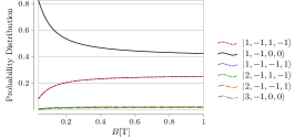
(c)

Figure 3.: LABEL:sub@fig:3a The energy levels of the spin Hamiltonian changing with the external magnetic field $B$. LABEL:sub@fig:3b The energy levels of the full spin-rotation Hamiltonian in Eq. 1 with $J_{\mathrm{max}}=4$. LABEL:sub@fig:3c The main probability distribution of the ground state on base kets $\ket{Jm_{J}k_{J}k_{K}}$ with $J_{\mathrm{max}}=4$.

III.3 Numerical results on eigen energies

Before numerical solving the eigen problem of Hamiltonian $H$, we first need to give the values of the inertia momentum $\{I_{1},I_{2},I_{3}\}$, which is determined by the nanodiamond size. In our calculations, we takes the bottom side length of the nanodiamond $a=$1\text{\,}\mathrm{nm}$$ and height $h=$1.225\text{\,}\mathrm{nm}$$, which leads to $I_{1}=$5.06\text{\times}{10}^{-44}\text{\,}\mathrm{k}\mathrm{g}\,\mathrm{m}^{2}$$ and $I_{3}=$3.11\text{\times}{10}^{-44}\text{\,}\mathrm{k}\mathrm{g}\,\mathrm{m}^{2}$$.

Since we focus on low energy physics of our system, it is nature to introduce a cutoff via a maximum angular momentum $J_{\text{max}}$ in our numerical calculations. To ensure the convergence of our physical results, we set $J_{\textrm{max}}=4$ (convergence tests see appendix B). Then we solve the eigen equation of full Hamiltonian

$$H|\Psi_{i}\rangle=E_{i}|\Psi_{i}\rangle,$$ (47)

where

$$|\Psi_{i}\rangle=\sum_{Jm_{J}k_{J}k_{K}}^{J\leq J_{\text{max}}}c^{(i)}_{Jm_{J}k_{J}k_{K}}\ket{Jm_{J}k_{J},Kk_{K}}.$$ (48)

The energy levels are shown in fig. 2b. As a comparison, fig. 2a shows the energy levels of the effective spin Hamiltonian

$$H_{S}=D\hat{S}_{z}^{2}+g\mu_{B}B\hat{{S_{z}}},$$ (49)

which generally describes a resting NV^- center with magnetic field $\vec{B}=B\vec{e}_{z}$ in NV^- axis.

From fig. 2a and fig. 2b, we observe that in different magnetic fields, the energies of the ground state for our system are similar as those of the Hamiltonian without considering the rotation given by Eq. 49. However, our ground states become highly entangled states which mainly involve six components as shown in fig. 2c.

IV Entanglement of thermal equilibrium state

When our quantum system interacts with its thermal environment, it will finally arrives at a steady state: the thermal equilibrium state. Now we are ready to study the entanglement properties in these thermal equilibrium states, which will be useful to guide us to provide a natural protocol to prepare entanglement between nanodiamond rotation and NV^- center spin.

IV.1 Entanglement of ground states

First we study the entanglement properties of the ground state, i.e., the thermal equilibrium state when the temperature limits to zero. For a ground state $\ket{G(B)}_{JS}$ at magnetic field $B$, the entanglement entropy is defined as:

$$S(\rho_{S}(B))=-\Tr_{S}\rho_{S}(B)\log_{2}(\rho_{S}(B)),$$ (50)

where $\rho_{S}(B)$ is the reduced spin density matrix of $\ket{G(B)}_{JS}$. Because the dimension of the Hilbert space of NV^- center spin $d_{S}=3$, the entanglement entropy $S(\rho_{S})\leq\log_{2}3$, where the equality is taken if and only if the ground state $\ket{G(B)}_{JS}$ is maximally entangled.

Numerical results on the entanglement entropy $S(\rho(B))$ are shown in fig. 3a. With the increasing of magnetic field $B$, the entanglement of the ground state grows from $0$ to approximately $\log_{2}3$, which implies that the ground state limits to a highly entangled state in a large magnetic field $B$.

IV.2 Entanglement of thermal equilibrium states at low temperatures

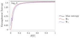
(a)

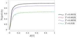
(b)

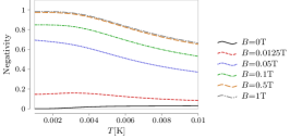
(c)

Figure 4.: The size of the particle is about $a=$1\text{\,}\mathrm{nm}$$. LABEL:sub@fig:4a The entanglement entropy of the ground sate and the first excited state compared with the maximum entanglement entropy for the maximum angular quantum number $J_{\textrm{max}}=4$. The negativity of the thermal entanglement state changing with magnetic field $B$ at some fixed temperatures $T$ LABEL:sub@fig:4b and with absolute temperature at some fixed magnetic fields $B$ LABEL:sub@fig:4c.

At temperature $T$, the thermal equilibrium state can be represented as

$$\rho_{JS}(B,T)=\frac{1}{Z}\sum_{i}e^{-\beta E_{i}}|\Psi_{i}\rangle\langle\Psi_{i}|,$$ (51)

where the partition function

$$Z=\sum_{i}e^{-\beta E_{i}},$$ (52)

and $|\Psi_{i}\rangle$ is the eigenvector of $H$ with eigenvalue $E_{i}$, which has been obtained numerically in the previous section.

Because the thermal equilibrium state $\rho_{JS}(B,T)$ is a mixed state, its entanglement can not be characterized by the entanglement entropy $S(\rho_{S})$, which is valid for characterization of entanglement for pure states. To study the entanglement property of the thermal equilibrium state, we introduce another entanglement measure, negativity [28, 29]

$$\mathcal{N}(\rho_{JS})=\sum_{\lambda<0}\mid\lambda\mid=\frac{\norm{\rho_{JS}^{T_{S}}}_{1}-1}{2},$$ (53)

where $\rho_{JS}^{T_{S}}$ is the partial transpose of spin index for the bipartite mixed state $\rho_{JS}$, $\lambda$ is the eigenvalue of $\rho_{JS}^{T_{S}}$. The negativity corresponds to the absolute value of the sum of negative eigenvalues of $\rho_{JS}^{T_{S}}$. $\norm{\rho_{JS}^{T_{S}}}_{1}$ is the trace norm of $\rho_{JS}^{T_{A}}$. The negativity $\mathcal{N}$ is a computable measure of entanglement for a mixed state and vanishes for separable states.

The numerical results of the negativity are shown in section IV.2. It is observed in fig. 3b that for a given temperature $T$, the negativity increases asymptotically to a maximum value with increasing of the magnetic field $B$. The temperature lower, the maximal value of the negativity larger. As shown in fig. 3c, for a fixed magnetic field $B$, the negativity decreases with increasing of the absolute temperature $T$. The magnetic field larger, the negativity larger. Our numerical results show that to obtain a thermal equilibrium state highly entangled, we need to increase the magnetic field larger than $0.5\text{\,}\mathrm{T}$ and decrease the temperature below $2\text{\,}\mathrm{mK}$.

Based on the above numerical results, we propose a simple protocol to asymptotically prepare a highly entangled state between mechanical rotation of the nanodiamond and the electron spin of NV^- center. First, cool down the system to below $2\text{\,}\mathrm{mK}$ at zero or weak external magnetic field strength. Then adiabatically boost the magnetic field strength to above $B=$0.5\text{\,}\mathrm{T}$$ and keep the system still in low enough temperature. Finally in thermal equilibrium, we get the thermal equilibrium state highly entangled.

V Discussion and conclusion

Our model is solved in the body-fixed frame, giving different results with which solved in the space-fixed frame as shown in section V. Because in space-fixed frame, the complete set of commuting observables is $\{\hat{{\bf\it L}}^{2},\hat{L}_{3},\hat{L}^{\prime}_{3},\hat{{\bf\it S}}^{2},\hat{S}_{3}\}$ which is not all commutative with those in the body-fixed frame, i.e. $\{\hat{{\bf\it J}}^{2},\hat{J}_{3},\hat{J}^{\prime}_{3},\hat{{\bf\it K}}^{2},\hat{K}^{\prime}_{3}\}$. This is consistent with physical interpretation that in the space-fixed frame strong enough magnetic field makes the spin occupying $\ket{-1}$ in ground state. Then from the view point in space-fixed frame, boosting magnetic field strength just results oppsite effect–disentangelment–comparing with the view in the body-fixed frame. More details see appendix C.

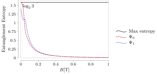
Figure 5.: The entanglement entropy of the ground state and the first excited state solved in the space-fixed frame with cutoff $L_{\mathrm{max}}=4$.

We propose a theoretical model to describe a rotating nanodiamond with an embedded NV^- center manipulated by a static external magnetic field. We neglect several factors in real experiments such as trap potential design, gravity effect, decoherence from external noises that may affect the accuracy of our model, which deserve further studies in future.

In our protocol to prepare entanglement, we propose to adiabatically boost the magnetic field strength. Theoretically, however, we do not require the boosting is adiabatic, a sudden change of the magnetic field strength may also work after a much longer equilibrium time.

In conclusion, we explore the entanglement properties of a rotating nanodiamond with an embedded NV^- center in an external magnetic field in a thermal equilibrium state, which includes the ground state as a special case. We find that the entanglement between nanodiamond rotation and NV^- center spin can be controlled by an external magnetic field and the temperature: larger magnetic field strength and lower temperature, more entanglement between the rotation and the spin. Our numerical results show that in our system setting when the magnetic field strength is tuned above $0.5\text{\,}\mathrm{T}$ and the temperature is controlled below $2\text{\,}\mathrm{mK}$, the thermal equilibrium state will be an almost maximally entangled state. Thus we propose a theoretical protocol to realize the highly entangled states of the spin-rotation coupled system asymptotically. The entanglement between the spin (a microscopic degree) and the rotation (a mesoscopic degree) is not only of interest in fundamental problems of quantum mechanics such as the border between quantum world and classical world [30], but also may find potential use in quantum control, and in quantum sensing and in quantum network.

Appendix A $D$-matrix and Euler rotations

In this appendix, we give some details of the $D-$matrix of Euler rotations. We have chosen $\{\vec{e}_{1},\vec{e}_{2},\vec{e}_{3}\}$ to represent the space-fixed frame and $\{\vec{e}^{\prime}_{1},\vec{e}^{\prime}_{2},\vec{e}^{\prime}_{3}\}$ the body-fixed frame. In the view of passive rotations, we consider $\vec{e}^{\prime}_{i}$ is rotated to $\vec{e}_{i}$ by rotation operator $\hat{R}$,

$$\vec{e}_{i}=\hat{R}\vec{e}^{\prime}_{i}=\sum_{j=1}^{3}R_{ji}\vec{e}^{\prime}_{j},$$ (A.1)

where

$$R_{ji}\equiv\vec{e}^{\prime}_{j}\dotproduct\vec{e}_{i}.$$ (A.2)

While in the view of active rotations, we usually define the rotation operator as $\vec{e}^{\prime}_{i}=\hat{Q}\vec{e}_{i}$ which maps a vector $\vec{e}_{i}$ to a new vector $\vec{e}^{\prime}_{i}$ in the same frame. It is clear to see that $\hat{R}=\hat{Q}^{-1}$ which usually gives the inverse relation of passive and active view of the same rotation transformation. In our paper, we choose the passive view on account of that we have defined two coordinate frames. And we choose Euler angles $\{\alpha,\beta,\gamma\}$ to represent the rotation from space-fixed frame $\{\vec{e}_{1},\vec{e}_{2},\vec{e}_{3}\}$ to body-fixed frame $\{\vec{e}^{\prime}_{1},\vec{e}^{\prime}_{2},\vec{e}^{\prime}_{3}\}$ which are shown in section II.

According to quantum mechanics, the generator of $\hat{R}$ is angular momentum $\hat{{\bf\it L}}$, especially in space-fixed frame,

$$\commutator{\hat{L}_{i}}{\hat{L}_{j}}=i\hbar\epsilon_{ijk}\hat{L}_{k},$$ (A.3)

where $i,j,k\in\{1,2,3\}$ with $\hat{L}_{i}\equiv\vec{e}_{i}\dotproduct\hat{{\bf\it L}}$ and $\epsilon_{ijk}$ is an antisymmetric tensor with $\epsilon_{123}=1$. Let $\hat{D}$ be the representation of the rotation operator $\hat{R}$ in Hilbert space, we have

$$\hat{D}(\alpha,\beta,\gamma)=\exp(\frac{i\gamma\hat{L}_{3}}{\hbar})\exp(\frac{i\beta\hat{L}_{2}}{\hbar})\exp(\frac{i\alpha\hat{L}_{3}}{\hbar}).$$ (A.4)

And the space base kets relations are defined as

$$\hat{D}^{\dagger}(\alpha,\beta,\gamma)\ket{\{\vec{e}^{\prime}_{i}\}}=\ket{\{\hat{R}\vec{e}^{\prime}_{i}\}}=\ket{\{\vec{e}_{i}\}}.$$ (A.5)

In particular, for any vector operator $\hat{{\bf\it A}}$

$$\hat{D}^{\dagger}\hat{{\bf\it A}}\hat{D}=\hat{Q}^{-1}\hat{{\bf\it A}}=\hat{R}\hat{{\bf\it A}}.$$ (A.6)

Then

$$\hat{D}^{\dagger}\hat{A}_{i}\hat{D} =\vec{e}_{i}\dotproduct\hat{D}^{\dagger}\hat{{\bf\it A}}\hat{D}$$

$$=\vec{e}_{i}\dotproduct\hat{R}\hat{{\bf\it A}}$$

$$=\vec{e}_{i}\dotproduct\sum_{j}(\hat{{\bf\it A}}\dotproduct\vec{e}^{\prime}_{j})\hat{R}\vec{e}^{\prime}_{j}$$

$$=\sum_{j}\hat{A}^{\prime}_{j}\vec{e}_{i}\dotproduct\vec{e_{j}}$$

$$=\hat{A}^{\prime}_{i}.$$ (A.7)

Since in the space-fixed frame, $\hat{\vec{e}}^{\prime}_{l}$ is a vector operator,

$$\commutator{\hat{L}_{i}}{\vec{e}_{j}\dotproduct\hat{\vec{e}}^{\prime}_{l}}=i\hbar\epsilon_{ijk}\vec{e}_{k}\dotproduct\hat{\vec{e}}^{\prime}_{l}.$$ (A.8)

More importantly, with the definition

$$\hat{L}^{\prime}_{i}\equiv\hat{\vec{e}}^{\prime}_{i}\dotproduct\hat{{\bf\it L}},$$ (A.9)

we have the following relations,

$$\commutator{\hat{L}_{i}}{\hat{L}^{\prime}_{j}} =0,$$ (A.10)

$$\commutator{\hat{L}^{\prime}_{i}}{\hat{L}^{\prime}_{j}} =-i\hbar\epsilon_{ijk}\hat{L}^{\prime}_{k}.$$ (A.11)

Given the eigenstates $\ket{LMK}$ of $\{\hat{{\bf\it L}}^{2},\hat{L}_{3},\hat{L}^{\prime}_{3}\}$, the eigenfunctions are

$$\bra{\{\vec{e}_{i}\}}\ket{LMK}=\bra{\{\hat{R}\vec{e}^{\prime}_{i}\}}\ket{LMK}$$ (A.12)

$$=\bra{\{\vec{e}^{\prime}_{i}\}}\hat{D}\ket{LMK}$$ (A.13)

$$=\sum_{M^{\prime}K^{\prime}}\bra{\{\vec{e}^{\prime}_{i}\}}\ket{LM^{\prime}K^{\prime}}\bra{LM^{\prime}K^{\prime}}\hat{D}\ket{LMK}$$ (A.14)

$$=\sum_{M^{\prime}}\bra{\{\vec{e}^{\prime}_{i}\}}\ket{LM^{\prime}K}\bra{LM^{\prime}K}\hat{D}\ket{LMK}$$ (A.15)

$$=\sum_{M^{\prime}}\bra{\{\vec{e}^{\prime}_{i}\}}\ket{LM^{\prime}K}\bra{LM^{\prime}K}\hat{D}\ket{LMK}\delta_{M^{\prime}K}$$ (A.16)

$$=\bra{\{\vec{e}^{\prime}_{i}\}}\ket{LKK}\bra{LKK}\hat{D}\ket{LMK}$$ (A.17)

$$=\bra{\{\vec{e}^{\prime}_{i}\}}\ket{LKK}\bra{LK}\hat{D}\ket{LM}.$$ (A.18)

From Eq. A.14 to Eq. A.15, we have used the communication relations Eq. A.10. The Eq. A.16 is valid because

$$\bra{LM^{\prime}K}\hat{L}_{3}\hat{D}\ket{LMK} =M^{\prime}\bra{LM^{\prime}K}\hat{D}\ket{LMK}$$

$$=\bra{LM^{\prime}K}\hat{D}\hat{D}^{\dagger}\hat{L}_{3}\hat{D}\ket{LMK}$$

$$=\bra{LM^{\prime}K}\hat{D}\hat{L}^{\prime}_{3}\ket{LMK}$$

$$=K\bra{LM^{\prime}K}\hat{D}\ket{LMK},$$ (A.19)

i.e.

$$\bra{LM^{\prime}K}\hat{D}\ket{LMK}=\bra{LM^{\prime}K}\hat{D}\ket{LMK}\delta_{M^{\prime}K}.$$ (A.20)

When the rotations are described by Euler angles,

$$\bra{LK}\hat{D}\ket{LM}=D^{(L)}_{KM}(\alpha,\beta,\gamma),$$ (A.21)

and Eq. A.18 gives us the eigenfunction Eq. 36.

Appendix B convergence tests

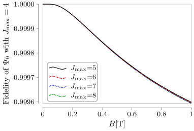
(a) The ground states.

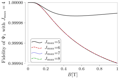
(b) The first excited states.

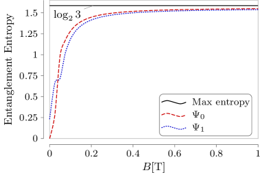
(c) Pure states.

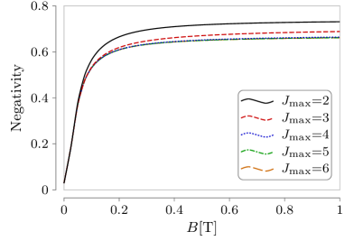
(d) Thermal equilibrium states.

Figure 6.: The fidelity between the LABEL:sub@fig:gs_fidelity ground states (LABEL:sub@fig:1e_fidelity 1-st excited states) of $J_{\mathrm{max}}=4$ and $J_{\mathrm{max}}\in\{5,6,7,8\}$. LABEL:sub@fig:entro_L8 The entanglement entropy of the ground state and the 1-st excited state with cutoff $J_{\mathrm{max}}=8$. LABEL:sub@fig:neg_Lmax2-6 The negativity of the thermal equilibrium states with different cutoff $J_{\mathrm{max}}\in\{2,3,4,5,6\}$ at temperature $T=$10\text{\,}\mathrm{m}\mathrm{K}$$.

In this appendix, we display the convergence tests of the cutoff of maximum angular momentum $J_{\mathrm{max}}$ in our numerical calculation.

Fidelity is a measure of the ”closeness” of two quantum states and is defined as the quantity

$$F(\rho,\sigma)=\biggl{(}\mathrm{tr}\sqrt{\sqrt{\rho}\sigma\sqrt{\rho}}\biggr{)}^{2}.$$ (B.1)

In the special case where $\rho$ and $\sigma$ are pure quantum sates, namely, $\rho=|\psi_{\rho}\rangle\langle\psi_{\rho}|$ and $\sigma=|\psi_{\sigma}\rangle\langle\psi_{\sigma}|$, the definition reduces to the squared overlap between the states:

$$F(\rho,\sigma)=|\langle\psi_{\rho}|\psi_{\sigma}\rangle|^{2}.$$ (B.2)

We check the fidelity between the ground states of $J_{\mathrm{max}}=4$ and $J_{\mathrm{max}}\in\{5,6,7,8\}$ as shown in fig. 5a, and see that the ground state of larger cutoff ($J_{\mathrm{max}}\geq 4$) changes very little. The case of the 1-st excited state shown in fig. 5b is the same.

As a comparison with fig. 3a which shows the entanglement entropy with a cutoff of angular momentum $J_{\mathrm{max}}=4$, a cutoff of $J_{\mathrm{max}}=8$ is shown in fig. 5c. For the thermal equilibrium states, we check their negativity with several cutoff $J_{\mathrm{max}}\in\{2,3,4,5,6\}$ at temperature $T=$10\text{\,}\mathrm{m}\mathrm{K}$$ which is shown in fig. 5d. It is clear to see that the negativity is convergent for $J_{\mathrm{max}}\geq 4$.

Appendix C Hamiltonian in space-fixed frame

In this appendix, we give a calculation of the model solved in space-fixed frame $\{\vec{e}_{1},\vec{e}_{2},\vec{e}_{3}\}$. A direct calculation shows that the complete set of commuting observables should be $\{\hat{{\bf\it L}}^{2},\hat{L}_{3},\hat{L}^{\prime}_{3},\hat{{\bf\it S}}^{2},\hat{S}_{3}\}$, and the Hamiltonian is written as

$$H =\frac{D}{\hbar}(\sum_{i=1}^{3}\hat{S}_{i}\vec{e}_{i}\dotproduct\vec{e}^{\prime}_{3})^{2}+\frac{1}{2}\frac{\hat{{\bf\it L}}^{2}}{I_{1}}+\frac{1}{2}\biggl{(}\frac{1}{I_{3}}-\frac{1}{I_{1}}\biggr{)}{\hat{L}_{3}^{\prime 2}}$$

$$\quad+\frac{g\mu_{B}}{\hbar}B\hat{S}_{3}.$$ (C.1)

One can solve the eigen problem of this Hamiltonian following the same procedure in the main text. The entanglement is between the NV^- spin and the mechanical rotation of the nanodiamond which is shown in section V.

References

- Doherty et al. [2013] M. W. Doherty, N. B. Manson, P. Delaney, F. Jelezko, J. Wrachtrup, and L. C. L. Hollenberg, The nitrogen-vacancy colour centre in diamond, Physics Reports The Nitrogen-Vacancy Colour Centre in Diamond, 528, 1 (2013).
- Chu and Lukin [2017] Y. Chu and M. D. Lukin, Quantum optics with nitrogen-vacancy centres in diamond, in Quantum Optics and Nanophotonics, edited by C. Fabre, V. Sandoghdar, N. Treps, and L. F. Cugliandolo (Oxford University PressOxford, 2017) 1st ed., pp. 229–270.
- Awschalom et al. [2018] D. D. Awschalom, R. Hanson, J. Wrachtrup, and B. B. Zhou, Quantum technologies with optically interfaced solid-state spins, Nature Photonics 12, 516 (2018).
- Gieseler et al. [2012] J. Gieseler, B. Deutsch, R. Quidant, and L. Novotny, Subkelvin Parametric Feedback Cooling of a Laser-Trapped Nanoparticle, Physical Review Letters 109, 103603 (2012).
- Delić et al. [2020] U. Delić, M. Reisenbauer, K. Dare, D. Grass, V. Vuletić, N. Kiesel, and M. Aspelmeyer, Cooling of a levitated nanoparticle to the motional quantum ground state, Science 367, 892 (2020).
- Tebbenjohanns et al. [2021] F. Tebbenjohanns, M. L. Mattana, M. Rossi, M. Frimmer, and L. Novotny, Quantum control of a nanoparticle optically levitated in cryogenic free space, Nature 595, 378 (2021).
- Yin et al. [2013] Z.-q. Yin, T. Li, X. Zhang, and L. M. Duan, Large quantum superpositions of a levitated nanodiamond through spin-optomechanical coupling, Physical Review A 88, 033614 (2013).
- Yin et al. [2015] Z. Yin, N. Zhao, and T. Li, Hybrid opto-mechanical systems with nitrogen-vacancy centers, Science China Physics, Mechanics & Astronomy 58, 1 (2015).
- Wan et al. [2016] C. Wan, M. Scala, G. W. Morley, A. A. Rahman, H. Ulbricht, J. Bateman, P. F. Barker, S. Bose, and M. S. Kim, Free Nano-Object Ramsey Interferometry for Large Quantum Superpositions, Physical Review Letters 117, 143003 (2016).
- Pedernales et al. [2020] J. S. Pedernales, G. W. Morley, and M. B. Plenio, Motional Dynamical Decoupling for Interferometry with Macroscopic Particles, Physical Review Letters 125, 023602 (2020).
- Arita et al. [2013] Y. Arita, M. Mazilu, and K. Dholakia, Laser-induced rotation and cooling of a trapped microgyroscope in vacuum, Nature Communications 4, 2374 (2013).
- Hoang et al. [2016] T. M. Hoang, Y. Ma, J. Ahn, J. Bang, F. Robicheaux, Z.-Q. Yin, and T. Li, Torsional Optomechanics of a Levitated Nonspherical Nanoparticle, Physical Review Letters 117, 123604 (2016).
- Kuhn et al. [2017a] S. Kuhn, A. Kosloff, B. A. Stickler, F. Patolsky, K. Hornberger, M. Arndt, and J. Millen, Full rotational control of levitated silicon nanorods, Optica 4, 356 (2017a).
- Kuhn et al. [2017b] S. Kuhn, B. A. Stickler, A. Kosloff, F. Patolsky, K. Hornberger, M. Arndt, and J. Millen, Optically driven ultra-stable nanomechanical rotor, Nature Communications 8, 1670 (2017b).
- Rashid et al. [2018] M. Rashid, M. Toroš, A. Setter, and H. Ulbricht, Precession Motion in Levitated Optomechanics, Physical Review Letters 121, 253601 (2018).
- Delord et al. [2017] T. Delord, L. Nicolas, Y. Chassagneux, and G. Hétet, Strong coupling between a single nitrogen-vacancy spin and the rotational mode of diamonds levitating in an ion trap, Physical Review A 96, 063810 (2017).
- Delord et al. [2020] T. Delord, P. Huillery, L. Nicolas, and G. Hétet, Spin-cooling of the motion of a trapped diamond, Nature 580, 56 (2020).
- Stickler et al. [2018] B. A. Stickler, B. Papendell, S. Kuhn, B. Schrinski, J. Millen, M. Arndt, and K. Hornberger, Probing macroscopic quantum superpositions with nanorotors, New Journal of Physics 20, 122001 (2018).
- Stickler et al. [2021] B. A. Stickler, K. Hornberger, and M. S. Kim, Quantum rotations of nanoparticles, Nature Reviews Physics 3, 589 (2021).
- Perdriat et al. [2022] M. Perdriat, P. Huillery, C. Pellet-Mary, and G. Hétet, Angle Locking of a Levitating Diamond Using Spin Diamagnetism, Physical Review Letters 128, 117203 (2022).
- Rusconi et al. [2022] C. C. Rusconi, M. Perdriat, G. Hétet, O. Romero-Isart, and B. A. Stickler, Spin-Controlled Quantum Interference of Levitated Nanorotors, Physical Review Letters 129, 093605 (2022).
- Chitambar and Gour [2019] E. Chitambar and G. Gour, Quantum resource theories, Reviews of Modern Physics 91, 025001 (2019).
- Biedenharn and Louck [1981] L. C. Biedenharn and J. D. Louck, Angular Momentum in Quantum Physics: Theory and Application, Encyclopedia of Mathematics and Its Applications ; Section, Mathematics of Physics No. v. 8 (Addison-Wesley Pub. Co., Advanced Book Program, Reading, Mass, 1981).
- Landau and Lifshitz [2013] L. D. Landau and E. M. Lifshitz, Quantum Mechanics: Non-Relativistic Theory, Vol. 3 (Elsevier, 2013).
- Yamanouchi [2012] K. Yamanouchi, Quantum Mechanics of Molecular Structures (Springer Berlin Heidelberg, Berlin, Heidelberg, 2012).
- Loubser and van Wyk [1978] J. H. N. Loubser and J. A. van Wyk, Electron spin resonance in the study of diamond, Reports on Progress in Physics 41, 1201 (1978).
- Rusconi and Romero-Isart [2016] C. C. Rusconi and O. Romero-Isart, Magnetic rigid rotor in the quantum regime: Theoretical toolbox, Physical Review B 93, 054427 (2016).
- Vidal and Werner [2002] G. Vidal and R. F. Werner, Computable measure of entanglement, Physical Review A 65, 032314 (2002).
- Horodecki et al. [2009] R. Horodecki, P. Horodecki, M. Horodecki, and K. Horodecki, Quantum entanglement, Reviews of Modern Physics 81, 865 (2009).
- Aspelmeyer et al. [2014] M. Aspelmeyer, T. J. Kippenberg, and F. Marquardt, Cavity optomechanics, Reviews of Modern Physics 86, 1391 (2014).