Optimal quantum speed for mixed states
Abstract
The question of how fast a quantum state can evolve is considered. Using the definition of squared speed based on the Euclidean distance given in [Phys. Rev. Research, 2, 033127 (2019)], we present a systematic framework to obtain the optimal speed of a -dimensional system evolved unitarily under a time-independent Hamiltonian. Among the set of mixed quantum states having the same purity, the optimal state is obtained in terms of its purity parameter. We show that for an arbitrary , the optimal state is represented by a -state with an additional property of being symmetric with respect to the secondary diagonal. For sufficiently low purities for which the purity exceeds the purity of maximally mixed state by at most , the only nonzero off-diagonal entry of the optimal state is , corresponding to the transition amplitude between two energy eigenstates with minimum and maximum eigenvalues, respectively. For larger purities, however, whether or not the other secondary diameter entries take nonzero values depends on their relative energy gaps . The effects of coherence and entanglement, with respect to the energy basis, are also examined and found that for optimal states both resources are monotonic functions of purity, so they can cause speed up quantum evolution leading to a smaller quantum speed limit. Our results show that although the coherence of the states is responsible for the speed of evolution, only the coherence caused by some off-diagonal entries located on the secondary diagonal play a role in the fastest states.
I Introduction
The maximum speed of evolution of a quantum system is a fundamental and important concept that has many applications in many areas of physics such as quantum communication BekensteinPRL1981 , quantum computation LloydN2000 , quantum metrology GiovannettiNP2011 , and optimal control CanevaPRL2009 . The quantum speed limit (QSL) then provides a lower bound on the time required to evolve an initial state to a target state under the Hamiltonian
| (1) |
For isolated systems, the QSL between two orthogonal states is defined as the maximum of the Mandelstam-Tamm (MT) bound MandelstamJP1945 and the Margolus-Levitin (ML) bound MargolusPD1998 , i.e.,
| (2) |
Above, the MT bound depends on the variance of the energy of the initial state and the ML bound depends on the mean energy with respect to the ground state, i.e., under the assumption that the energy of the ground state is taken to be zero. Levitin and Toffoli proved that the combined bound of MT and ML is tight and can only be attained by two-level state where and is an arbitrary phase LevitinPRL2009 . They have also shown that no mixed state can have a larger speed.
The QSL was originally derived for the unitary evolution of pure and orthogonal states and is then generalized to the arbitrary angles GiovannettiPRA2003 , mixed states GiovannettiPRA2003 ; WuPRA2018 ; CampaioliPRL2018 , and nonunitary evolutions TaddeiPRL2013 ; delCampoPRL2013 ; DeffnerPRL2013 . There are also some researches on the relationship between the QSL and the quantum phenomena such as the role of entanglement in dynamical evolution GiovannettiEU2003 ; BatlePRA2005 ; ZanderJPA2007 ; FrowisPRA2012 ; BorrasPRA2006 ; KupfermanPRA2008 , non-Markovian effect of the environment on the speed of quantum evolution DeffnerPRL2013 ; CianciarusoPRA2017 , and dependence of the QSL on the initial state WuJPA2015 ; LiuPRA2015 . Very recently, the QSL has also been used to derive lower bounds on the minimal time required to vary (generation and degradation) a quantum resource CampaioliNJP2022 , the informational measures MohanNJP2022 , and the correlations PandeyPRA2023 of quantum systems under some quantum dynamical process. It was also used to interpret the geometric measure of multipartite entanglement for pure states as the minimal time necessary to unitarily evolve a given quantum state to a separable one RudnickiPRA2021 .
Among the three elements of , namely , and , in most QSL discussions it is assumed that the Hamiltonian of the system is given and by fixing the distance between the initial and final states, the evolution time is bounded for any arbitrary state according to the chosen metric FreyQINP2016 . The MT and ML bounds are of this type. The evolution time, however, can be framed and studied in various other ways. In quantum control, for instance, the task is to search for the optimal Hamiltonian to drive the physical system between given initial and final quantum states in the shortest time. Finding the time-optimal evolution is analogous to that for the brachistochrone in classical mechanics and determines the optimal Hamiltonian and the type of control as the physical resources needed to carry out the process CarliniPRL2006 ; CarliniJPA2008 ; WangPRL2015 ; GengPRL2016 ; LamPRX2021 .
For the construction of QSL bounds, choosing a measure of distinguishability is, in general, necessary in order to be able to define the quantum speed as the derivative of some distance DeffnerJPA2017 . Various metrics have been used to obtain better bounds for QSL, for instance, del Campo et al. used the relative purity delCampoPRL2013 , Deffner and Lutz worked with Bures angle DeffnerPRL2013 , and Campaioli et al. defined a new distance based on the angle between generalized Bloch vectors CampaioliPRL2018 . Pires et al. have shown that there is an infinite family of contractive metrics that can be used to obtain QSL bounds PiresPRX2016 . Such bounds depend on the chosen metric and, in general, it is not easy to obtain a tight and attainable bound by the appropriate choice of the metrics. In more general cases, QSLs are loose for mixed states of unitary evolutions or open dynamics CampaioliQ2019 ; PiresPRX2016 . In particular, for pure states both MT and ML QSL bounds are attainable, however, for a general mixed state they can be rather loose. For instance, a state that is diagonal in the energy eigenbasis does not evolve further, so the speed of evolution is zero or, equivalently, is infinite. However, in this case, both the MT and ML lower bounds on can be arbitrarily small. This means, for incoherent states in the energy eigenbasis, and do not contain any information about the speed of evolution MarvianPRA2016 . In addition, any function that is used to quantify the speed of evolution is expected to be nonincreasing under mixing, however, the standard MT bound does not have this property, because the uncertainty in general increases under mixing. Motivated by these, Marvian et al. have found QSL bounds in terms of the coherence of states relative to the energy eigenbasis MarvianPRA2016 . Also, in PiresPRX2016 ; MondalPLA2016 the authors obtained bounds for in terms of skew information, as a measure of coherence. Another problem related to QSL bounds is the explicit dependence of many bounds on the time parameter ShaoPRR2020 . For a noncontrolled fixed Hamiltonian and by starting from a given initial state , the dynamical trajectory as well as the set of states satisfying the target angle is fixed, so that the QSL should not depend on the time either. Motivated by this, the authors of Ref. ShaoPRR2020 have defined the QSL time as the minimum evolution time to fulfill the target angle for any initial state that can fulfill the target angle .
The above discussion implies that the QSL requires more considerations, in particular for mixed states, so new approaches in the field can be effective and even necessary. Our main goal in this study is to find a tight and maximum speed for mixed states of the isolated systems. We survey directly on the evolution speed instead of the evolution time, therefore, we do not face the problem of the explicit dependence of the QSL on the time parameter. The notion of speed depends on the choice of metric on the space of quantum states, each of which has its own figure of merit depending on the desired purpose and application. In this work, we adapt the notion of speed based on the Euclidean metric defined naturally on the Hilbert-Schmidt space in the Bloch vector representation of the quantum states BrodyPRR2019 . This choice of metric provides a simple form for speed in terms of instead of which appears in the squared speed based on the Wigner-Yanase (WY) skew information MondalPLA2016 ; PiresPRX2016 , so making our calculations computable. The defined speed vanishes for all incoherent states, and even more, it is convex under mixing thus speed does not increase under mixing.
We restrict ourselves to the unitary evolution generated by the time-independent Hamiltonian. In this case, the speed remains constant in time, regardless of what initial state the system starts in and how far the distance between and is. The speed therefore depends only on the initial state. Our aim is to express this dependence in terms of purity; for instance, zero speed for maximally mixed state and maximum speed for the pure state . Motivated by this, we pursue then the question that among the set of all quantum states with a given definite purity, which initial state represents the optimal one. By parameterizing an arbitrary -dimensional mixed state in terms of its purity, we identify the state with maximum speed for each given purity. Such obtained optimal state provides a tight bound for the QSL induced by the Euclidean metric. We apply our optimal states to the squared speed defined by the WY skew information MondalPLA2016 ; PiresPRX2016 . The numerical simulations show that the proposed optimal state provides almost a faster squared speed, except for some region of low purity for which the speed exceeds the speed limit proposed by our optimal state. In such cases, however, our optimal state can be exploited in order to derive lower bounds for the maximum speed.
Our other important result is that although the off-diagonal entries of a quantum state play a key role both in the quantum coherence of the state and in the speed of quantum evolution, their influences do not match with each other in general. In other words, despite the coherence of the initial state can speed up the quantum evolution process, for the optimal states only the coherence arisen from the secondary diameter of the state can have a nonzero contribution in the optimal speed, all other off-diagonal entries have vanishing contributions. Furthermore, for all density matrices with arbitrary purity, the entry always has a nonzero contribution on the optimal state. However, whether or not the other secondary diameter entries take nonzero values depends on their relative energy gaps .
For those dimensions characterizing a bipartite system with , we investigate the behavior of the optimal speed with respect to the entanglement of the optimal state. In doing so, we suppose the energy eigenstates provide a product basis, and we find that except for the sufficiently low purities, the optimal state has nonzero entanglement. Our results show in particular that for the case of an -qubit system for which , the one-qubit reduced state of the optimal state, obtained by tracing out qubits, is a maximally mixed state. When , for instance, the optimal states therefore form a special class of Bell-diagonal states, up to a local unitary transformation. Furthermore, for optimal states both resources are monotonic functions of purity, so they can cause speed up quantum evolution leading to a smaller quantum speed limit.
The paper is organized as follows. In Section II, we first briefly review the squared speed of evolution of a -dimensional system with respect to the Euclidean metric defined in BrodyPRR2019 . Some related properties and preliminaries are given also in this section. Section III is devoted on the optimal speed of a mixed state with an arbitrary purity. Our main results, namely Proposition 5 and Theorems 6, 7 and 8 are presented in this section, however, some of their proofs can be found in Appendices A and B. A simulation evidence of our results is provided in Sec. IV. In this section we also apply our optimal states to the squared speed defined by WY skew information. The role of entanglement and coherence of the optimal states are discussed in Sec. V. The paper is concluded with a brief review in Sec. VI.
II Speed of quantum evolution
An arbitrary quantum state acting on the -dimensional Hilbert space can be written in the Bloch vector representation as
| (3) |
where , and are Hermitian traceless orthonormal basis, with the Hilbert-Schmidt inner product . In this representation , and is the Bloch vector corresponding to the state .
Starting from the initial state , consider a one-parameter family of states generated by an open system dynamics as
| (4) |
where the dissipator term
| (5) |
is responsible for the open dynamics of the system. Based on the above dynamics, the authors of Ref. BrodyPRR2019 obtained the squared speed of evolution with respect to the Euclidean metric as
| (6) |
which can be written as BrodyPRR2019
| (7) |
Clearly, the first and the second terms arise purely from unitary and dissipative dynamics of the evolution, respectively. The third term, on the other hand, comes from incompatibility between the Hamiltonian and the set of Lindblad operators BrodyPRR2019 .
II.1 Speed of unitary evolution
In this work, we consider only unitary evolutions. We also assume Hamiltonian is time-independent. With these assumptions, the squared speed for a closed system becomes time-independent and depends only on the initial state. So, if we find the optimal state initially, it remains optimal at later times as well.
Let denotes the orthonormal eigenbasis of the Hamiltonian corresponding to the eigenenergies , i.e. . In this basis, is represented by and Eq. (7) reads
| (8) | |||||
Above, in the natural units with , we have defined for as the Bohr frequency corresponding to the transition between lower and upper levels and , respectively. Clearly, obeys the sum rule . It follows from above relation that only the off-diagonal elements of , in the Hamiltonian bases, contribute to the speed of unitary evolution. Before we proceed further, it may be relevant to point out some properties of the squared speed.
II.2 Properties of the squared speed
Lemma 1.
Let and be two complementary orthogonal subspaces of on which the Hamiltonian is partitioned into and , i.e., and . Then for any pair of orthogonal states and acting on and , respectively, we have
| (9) |
Proof.
Putting and in the first line of Eq. (8), and using the fact that for , one can easily obtain the equation above. ∎
Lemma 2.
The squared speed of unitary evolution is a convex function of , i.e., for any pair of states and and an arbitrary , we have
| (10) |
Moreover, the inequality is saturated if and only if, in the Hamiltonian basis, the off-diagonal elements of and are likewise equal, for .
Proof.
To prove the lemma, note that the first line of Eq. (8) can be written also as
| (11) |
where is the Hilbert-Schmidt norm induced from the Hilbert-Schmidt inner product . In view of this, the convexity of the squared speed follows from the convexity of the Hilbert-Schmidt norm, i.e., for any pair of operators and , and , we have
Inserting and , we arrive at our assertion (10).
From , it follows that the inequality (II.2) is saturated if and only if , i.e., if and only if is diagonal in the Hamiltonian basis, implying that the off-diagonal elements of and are likewise equal, for . Note that, as only off-diagonal elements of a density matrix play a role in the speed, we have therefore , however, the converse is not true in general, i.e., it may happens that but the inequality (II.2) is not saturated. ∎
As we mentioned previously in Sec. I, this feature of convexity is crucial for any function that is used to quantify the speed of evolution in order to be nonincreasing under mixing MarvianPRA2016 . In Sec. III we see that the optimal speed is a monotonic function of the purity of the state.
Lemma 3.
For a general state , the squared speed is bounded from above by
| (13) |
where is the variance of . Moreover, the inequality is saturated if and only if the state is pure (see GessnerPRA2018 for a same relation for quantum Fisher information).
III Optimal-speed quantum states
Under the Hamiltonian , how fast can a quantum state evolve in time? In particular, which of the pure states is the fastest one or, even more, over the set of density matrices with equal purity, which states have the optimum speed? In what follows, we are going to address these questions by developing a framework to obtain the optimal state having definite purity.
III.1 Optimal pure quantum states
According to the Lemma 3, the squared speed of a pure state reduces to
| (16) |
In view of this, the following proposition introduces the states for which the energy variance is maxima TextorIJTP1978 ; Sakmann2011PRA , so the squared speed is maximum.
Proposition 4.
Let denotes the orthonormal eigenbasis of the Hamiltonian , corresponding to the nondecreasing ordered eigenvalues . Then the pure state makes the energy variance maximum if , where and are two states in the eigensubspaces of minimum and maximum energies and , respectively. Accordingly, the maximum value of the variance of and its corresponding maximum squared speed are and , respectively. Obviously, when both and are nondegenerate, the maximum variance happens for and , i.e. when .
III.2 Optimal mixed quantum states
For a general quantum state , acting on the -dimensional Hilbert space , one can define the purity as , where ranges from for the maximally mixed state to for an arbitrary pure state corresponding to the projection operator . In what follows, we are looking for a class of mixed states , parameterized by the associated purity , such that the squared speed is maximal. For , the result of the Proposition 4 is retrieved by a new approach.
In energy eigenbasis, the purity of a general state can be expressed as
| (17) |
For the maximally mixed state for which the speed is zero, we have . It follows therefore that in order to have nonzero speed, we have to increase the purity of state. Our goal is to increase the speed by increasing the purity in an optimum manner. A systematic framework to obtain the optimal states of a -dimensional system is presented by Theorems 6, 7 and 8 below. Their structural form, however, is given by the following proposition.
Proposition 5.
For an arbitrary dimension , the optimum state is given by a persymmetric -state, i.e., a -state which is symmetric with respect to the secondary diagonal so that for all
| (18) |
Here, in the innermost we have when is odd, and a two-dimensional persymmetric matrix when is even.
Proof.
The proof is provided in Appendix A. ∎
The following theorems determine the nonzero entries of the optimal state (18) for various values of purity.
Theorem 6.
For where
| (19) |
the optimal quantum state is given by
| (20) |
where . Obviously, the rank of the optimal state (20) is full except at for which the rank is diminished by 1, so that . Moreover, the optimal squared speed is .
Proof.
Our goal is to increase the speed by increasing the purity in an optimum manner. This is achieved if we let one or more off-diagonal elements of the density matrix to be increased. The diagonal elements of the density matrix do not play a role in the speed and among the set of all off-diagonal elements, plays a more important role than the others, as its absolute value appears as the coefficient of the largest squared energy gap in Eq. (8). Starting from the maximally mixed state which has minimum purity and vanishing speed, and by keeping all the parameters fixed except , we increase the speed by increasing under the restriction . In turn, the purity is increased to , or equivalently, the density matrix acquires the new off-diagonal entries for . We arrive therefore at the result asserted by Theorem 6 for the optimal state when . ∎
It is interesting to note here that the state given above is the same as the optimal state introduced recently in Ref. ShaoPRR2020 to fulfill the target via the operational definition of QSL. Our next goal is to find the optimum squared speed for the other values of purity, namely for . For and dimensions , the optimal state depends in general on the relative values of the Bohr frequencies . Let us define , , and so on. Obviously, . Then, Theorems 7 and 8 present the optimal states when and , respectively.
Theorem 7.
When , the optimal state is given by
| (21) |
for , where and
| (22) |
Proof.
For a proof see Appendix B.1. ∎
For , the calculations to specify the nonzero entries become more complicated, however, a framework to identify the optimal state can be developed. In this case, we need to define two purities and as
| (23) | |||||
| (24) |
Theorem 8.
When and depending on the value of , the optimal state can be obtained as follows.
-
•
For , the optimal state is still given by Eq. (21).
-
•
For , the optimal state is given by
where with as an arbitrary phase, and
(26) -
•
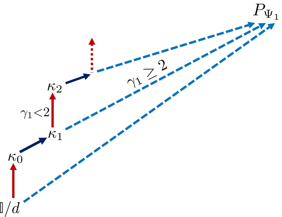
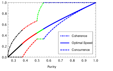
To proceed further for and to reach the maximum purity of unity, we must repeat steps similar to those used to derive Eq. (• ‣ 8). For more detail, we refer to step 4 of the proof. The calculations become more complicated due to the need to account for other threshold ratios such as , , and so on. However, for dimensions the only relevant threshold parameter is , as such the steps given above are exhaustive to obtain the optimal state. Figure 1 represents a schematic overview of how this framework works.
Proof.
A sketch of the steps to be followed is provided in Appendix B.2. ∎
III.3 Examples: optimal mixed quantum states for
After giving a framework to obtain the optimal states, in this subsection we present the optimal states for the first three simple but important cases and . We postpone their proof until we provide a proof sketch for our main theorems for a general in Appendix B.
III.3.1 Optimal mixed quantum states for
In this case, as demonstrated in Fig. 1, the optimal state is achieved by the first upright arrow, i.e., the path . Actually, since for , Theorem 6 presents the optimal squared speed of a qubit for the whole range . In this case, Eqs (8) and (20) give the optimal speed and its corresponding optimal state as and
| (27) |
respectively.
III.3.2 Optimal mixed quantum states for
For , we have to take the path . In this case, the state with optimal speed is given by
| (28) |
where is an arbitrary phase, and matrix entries , and are given in Table 1.
III.3.3 Optimal mixed quantum states for
For , the optimal state depends not only on the purity , but also on the relative values of the Bohr frequencies . In particular for , depending on whether is greater than or less than 2, we have to take the path or . In this case, the optimal state is given by
| (29) |
where its nonzero entries, depending on whether the threshold parameter is greater than or less than 2, are given in Table 2.
IV Simulation and comparison with WY skew information
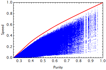
In this section we examine a numerical simulation performed on the squared speed (8) for . Our results show, as expected, that the optimal state (29) is always an upper bound for this speed. To generate a uniform distribution on the set of all -dimensional quantum states we follow the method presented in KarolPRA1998 . A general -dimensional quantum state can be represented by a diagonal density matrix and a unitary matrix as . Accordingly, one can proceed to construct the uniform density matrices through two steps: First, a uniform diagonal density matrix is generated by using a uniform distribution of probabilities. In the second route, we use a uniform distribution on unitary transformations , and generate a uniform density matrix . A simulation of the squared speed for is given in Fig. 2. To construct this figure, we generate one million random quantum states; ten thousand for random diagonal states and one hundred for random unitary matrices. Moreover, by choosing , we have normalized the optimal speed to unity in the sense that . Our results confirm that the squared speed is bounded from above by the analytical optimal squared speed given by Eq. (29) (the red curve).
Now, two comments are in order. (i) The figure shows a sparse distribution of the randomly generated states for large values of purity. This comes from the fact that the set of pure states is measure zero, as such, the probability of obtaining random diagonal pure states is zero. In light of this, the probability of generating randomly diagonal states with large purity is very small so that the density of generated states is reduced by increasing the purity . (ii) It follows from the figure that the optimal state (the red curve) is not reachable randomly, unless for low purities. This is evident from our result since the optimal state (18) is a -type state which is of measure zero among all quantum states. This implies that for the more complicated case of of high-dimensional systems where the numerical simulation is inevitable, the probability of finding the optimal state is almost zero unless the search is performed among the states which possess the -type form (18).
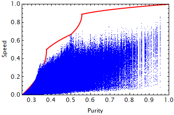
We have to stress here that the quantum speed, as well as the states with maximum speed, depends in general on the chosen metric. Accordingly, for the metrics other than the Euclidean metric that we have used in this work, state (18) is not guaranteed to be optimal for the whole values of purity. In such cases, however, Eq. (18) can be exploited in order to derive tight lower bounds for the maximum speed. To see this, let us examine the squared speed based on the Wigner-Yanase (WY) skew information MondalPLA2016 ; PiresPRX2016 , which takes the following form in our notation
| (30) |
This, clearly, is similar in form to the Euclidean-based squared speed (8), except that here the off-diagonal entries of are replaced by the ones of . Figure 3 shows a numerical simulation of this squared speed, plotted against the purity. The red curve, on the other hand, shows the squared speed (30), obtained for the state of Eq. (18). To obtain the red curve, we have used the fact that is again a persymmetric -state as Eq. (18), however, with the entries and where . Same relations hold for entries and in terms of and . Clearly, for some regions of low purity, the speed exceeds the speed limit proposed by our optimal state (18). This, in turn, implies that the state (18), which is optimal by means of the speed defined by Eq. (8), no longer remains optimal in general for other definitions of speed. Such optimal state, however, could shed some light on the QSL bounds.
V Discussion: Entanglement and coherence
It is understood that quantum resources such as entanglement and coherence could speed up quantum evolutions and in particular for unitary evolutions it is shown that entanglement can reduce the quantum speed limit time GiovannettiPRA2003 ; GiovannettiEU2003 ; BorrasPRA2006 . In this section we discuss the role played by these resources.
V.1 Entanglement
To study the effect of entanglement on the optimal speed, suppose the -dimensional system constitutes a bipartite system, i.e. so that where and are dimensions of and , respectively. We assume that the Hamiltonian is diagonal in the product basis so the energy eigenstates provide a product basis, i.e.,
| (31) |
This includes the Hamiltonians of the form BatlePRA2005
| (32) |
where and are local Hamiltonians of the subsystems and , respectively. To proceed further we first consider , i.e., a two-qubit system which is the simplest bipartite system described by a four-level model.
In this case the Hamiltonian is diagonal in the product basis , , , and . To quantify entanglement we use concurrence WoottersPRL1998 as a measure of entanglement which has a closed formula for two-qubit states. With the above assumption, the concurrence of the optimal state (29) is given by
| (33) |
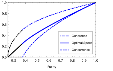
which interestingly is exactly equal to the negativity measure of entanglement defined by , where is a matrix defined by partial transposing PeresPRL1996 ; HorodeckiPLA1996 the quantum state with respect to the first part, and is the trace norm. Figures 4 and 5 illustrate the concurrence (below-dashed curve) of the optimal state in terms of the purity for two regimes and , respectively. It follows from these figures that in both cases the optimal state is disentangled for . On the other hand, for and in both regimes, the optimal state is no longer disentangled; its concurrence monotonically increases with purity.
For an arbitrary -dimensional composite system, with , we first show that the optimal state is separable for all purities . To see this one can easily check that the state given by Eq. (20) possesses the following representation in terms of product states
Here, the coefficients s are zero except for , and and are projections on pure states
| (35) | |||
of the first subsystem, and and are defined similarly for the second subsystem.
Remarkably, this separability of a bipartite state for low purities is not surprising as all states in the sufficiently small neighborhood of the maximally mixed state are necessarily separable. More precisely, any bipartite mixed state with purity less than has positive partial transposition KarolPRA1998 . Our result shows however a wider range of separability for the optimal state; the optimal state is separable for purities less than .
For , on the other hand, the optimal state for an arbitrary -dimensional composite system is always entangled. To see this, let us first consider the case for which the optimal state is given by Eq. (21). Simple calculation shows that the partial transposed matrix has positive eigenvalues, namely , and with multiplicities , and respectively, and one negative eigenvalue equal to . These eigenvalues are independent of how the composite system is partitioned into two subsystems and . Note that , defined by Eq. (22), is a monotonically increasing function of and ranges from to as goes from to . Accordingly, negativity is given by which is monotonically increasing in interval and reaches the maximum value of unity at .
In regime and for which more threshold ratios are needed to characterize the optimal state, calculation of the negativity becomes more complicated for . However, as we mentioned in Theorem 8, the optimal state is still given by Eq. (21) for , so that its negativity is still given by . In view of this, the optimal state starts to be entangled at purity for arbitrary . This entanglement increases monotonically in the interval and reaches the maximum value , where is defined by Eq. (26) (see Fig. 5 when ).
For the optimal state is given by Eq. (• ‣ 8), and can be rewritten as
where is a separable (unnormalized) state with a product representation similar to that given by Eq. (V.1). The spectrum of the partial transposed matrix has one negative eigenvalue leading therefore to the negativity which is equal to . This explains why the entanglement of the optimal state is constant in interval . This procedure can be continued until the purity tends to , corresponding to the optimal pure state which has the maximum value of unity for the negativity.
V.2 Coherence
According to the Eq. (8), the squared speed of a system evolved unitarily under the Hamiltonian is nonzero if and only if the system has nonzero coherence in the energy eigenbasis. However, despite the key role of coherence in the evolution speed of the system, not every increase in the coherence will result in an increase in the speed. We are also interested in to find out how the optimal speed is related to the coherence of the optimal state. To this aim, we use the -norm of coherence PlenioPRL2014
| (36) |
to quantify the coherence of in the Hamiltonian basis.
Figure 6 shows the numerical simulations of the squared speed plotted against the coherence for when . The simulations are conducted for four values of purity, corresponding to the four regions , , , and . For comparison, the optimal state associated with each purity is also drawn by a red point. It follows from these figures that the state with maximum coherence does not always result in the maximum speed. Moreover, the coherence of the optimal state is not even as large as the mean coherence of the randomly generated states.
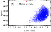
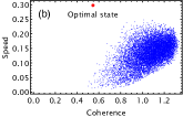
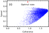
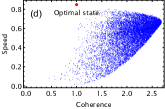
For the optimal state, given by Eq. (29) for , the -norm of coherence reduces simply to . Since the optimal states possess the -type symmetry, only the coherence caused by the secondary diameter entries and have a nonvanishing effect on the optimal speed, as such, the maximum value of the coherence could not exceed unity. Figures 4 and 5 illustrate the coherence, the speed, and the concurrence of the optimal state in terms of the purity for two regimes and , respectively. These figures depict the optimal speed as a monotonic function of both quantities and , however, the converse is not true in general as we already mentioned it in Figure 6 for the coherence.
A comparison of Figures 4 and 5 shows that when , all mentioned quantities are independent of the value of as we expect from Table 2. When moving away from the maximally mixed state , namely for , their behaviors become different, depending on whether the threshold ratio is greater than or less than 2. In particular, for , both coherence and concurrence have sudden changes at two purities and . At , the coherence increasing is suddenly accelerated, while the concurrence increasing is suddenly stopped. For , any increase in purity is consumed to increase the coherence to its maximum value of unity, while the concurrence maintains its constant value . At , on the other hand, the coherence increasing is suddenly stopped after reaching its maximum value of unity, while the concurrence starts to increase. For the remaining range of purity, i.e., for , their behavior becomes opposite in the sense that while coherence remains unchanged, the concurrence is increased in order to reach its maximum value of unity. These properties can have applications, for instance, in the real dynamics where the system-environment interaction is inevitable and the system loses its purity. In such cases, the optimal-speed dynamics can be utilized to reduce the operation time in order to maintain the quantum features such as quantum coherence and quantum entanglement.
Turning our attention to the definition of squared speed given by Eq. (8), one can interpret it as a competition between the energy gaps and the off-diagonal entries which have direct contribution to the quantum coherence (see Eq. (36)). In view of the above discussion, the role of energy gaps is dominant over the off-diagonal entries when , however, for the roles are reversed, i.e., the coherence plays a greater role than the energy gaps. Using the general definition of -norm of coherence, Eq. (36), a similar discussion can be made for the coherence of the -dimensional optimal state (18).
VI Conclusion
In this paper we have considered the question that how fast can a quantum state evolve or, more precisely, among the set of all quantum states with a given definite purity , which initial state represents the optimal one. Based on the notion of squared speed defined on the Euclidean metric BrodyPRR2019 , an analytical framework to obtain the optimal speed of a -dimensional system with unitary evolution generated by a time-independent Hamiltonian is presented. The framework works step-by-step in the sense that starting from the maximally mixed state having minimum purity and zero speed, the purity is increased optimally in favor of speed.
In any dimension , and for a given purity , the fastest state is a -state with an additional property that it is also symmetric with respect to the secondary diagonal. The off-diagonal entry has nonzero contribution to all optimal states with arbitrary purity . Other off-diagonal entries , however, can have a nonzero contribution to the optimal speed depending on the ratio of the Bohr frequencies. In particular for , where , all entries vanish except . In this regime, we have found a complete description of the optimal state for an arbitrary dimension .
On the other hand when , the off-diagonal entry makes a nonzero contribution to the optimal states for all purities where is given by Eq. (23). In this regime, we have presented a complete solution for . For higher dimensional systems, however, more threshold parameters are needed to decide whether or not the other off-diagonal entries have nonzero contribution in the optimal state, so that a general treatment to find the optimal state is more complicated.
Entanglement and coherence of the optimal states and their relations with purity have been also investigated. We have found that for the optimal states both resources are monotonic functions of purity. Although a nonzero coherence, in the energy eigenbasis, is a necessary and sufficient condition for the nonzero speed, any increase in the coherence, however, will not results in an increase in the speed. For the sufficiently low purities, namely for , the speed is independent of the value of , as such, both quantum coherence and quantum entanglement are independent of the value of . For , on the other hand, their behaviors become different depending on whether the threshold parameter is greater than or less than 2. In particular, both coherence and concurrence display sudden changes in their behaviors when , but it is not the case for . Moreover, our results show that the role of energy gaps is dominant over the off-diagonal entries when , however, for the coherence plays the dominant role.
These results could find applications in real dynamics where the system-environment interaction is inevitable and the system loses its purity. In such cases, the optimal-speed dynamics can be utilized to reduce the operation time in order to maintain quantum features such as quantum coherence and quantum entanglement. Having the states with maximum speed for each purity , they can be used to construct a tight QSL. Due to the widespread use of the QSL in diverse branches of quantum technology, it is hoped that our results should shed light on the several applications including quantum communication, quantum computation, quantum metrology, and especially quantum control.
In open dynamics the purity is not preserved in general, so the generalization of our method to open dynamics is not straightforward. In such systems, the radial component of the speed will obtain a nonvanishing contribution to the speed, leading therefore to the change of state purity. This component, which is expressed in terms of Lindblad operators, vanishes for a unitary evolution BrodyPRR2019 , so the purity remains constant. To obtain the fastest states in an open system, both radial and tangential components of the speed must be optimized simultaneously. This problem can be considered for future works.
acknowledgment
This work was supported by Ferdowsi University of Mashhad under Grant No. 3/55339 (1400/06/28).
Appendix A Proof of Proposition 5
The following two lemmas are essential in proving Proposition 5.
Lemma 9.
Suppose is a -dimensional density matrix, and is its 2-dimensional minor obtained by removing all rows and columns except rows and columns . If , then for . Moreover, vector belongs to , i.e. . Similarly, for all -order minors , , for which , then for .
Proof.
The positivity of requires that all -order () principal minors of be nonnegative. Consider the -order principal minors obtained by removing all rows and columns except rows and columns for a fixed value of . One can easily show that the determinant of this minor equals , which is negative unless . ∎
Lemma 10.
Suppose be a state with purity such that . If be a state with optimal speed, then for . In this case, and belongs to the support and kernel of , respectively, in the sense that and . This result is general in the sense that if for some , and be a state with optimal speed, then for . In this case, and belongs to the support and kernel of , respectively, in the sense that and .
Proof.
We provide a proof for the case of ; the proof for an arbitrary is similar. First note that the case gives immediately , a result obtained by nonnegativity of the determinant of , so we proceed with the assumption that . From Eq. (8) and applying Lemma 9, the squared speed of is given by
| (37) |
where for . The optimum squared speed is obtained by maximizing the above speed subject to the purity constraint where
| (38) |
Note that the squared speed is not a function of the diagonal elements , except for because of its relation to the off-diagonal element . Therefore, the normalization condition is not relevant as an equality condition, however, we should check the inequality together with the positivity condition at the end of our calculations.
Using the method of Lagrange multiplier, we have to maximize subject to the purity condition . Denoting by the corresponding Lagrange multiplier, and writing , we have the following relations from , (), and (), respectively
Since , the first relation determines the Lagrange multiplier as . Accordingly, for the second relation, is not an acceptable solution unless , which is not possible as ; as such, we provide a prove for the assertion that for the optimal state for . For the third relation, can be an acceptable solution in some particular cases, but we postpone its discussion while we provide proofs for Theorems 7 and 8. ∎
We are now in the position to proof the Proposition 5. That the optimality requires the state possess the -type symmetry is a consequence of the successive application of the Lemmas 9 and 10. The additional property of being symmetric with respect to the secondary diagonal, i.e., for all , comes from the Step 1 below.
Appendix B Proofs of Theorems 7 and 8
B.1 Proof of Theorem 7
To prove Theorems 7, we follow the following steps.
Step 1 ()
We start from Eq. (20) when reaches its maximum value , i.e.,
| (39) |
where is a state with maximum squared speed. Clearly no longer contains in its range, as such .
With such starting point, the squared speed can be increased by increasing the purity to via two strategies: (i) Increasing some off-diagonal entries except , but keeping the diagonal entries fixed. (ii) Increasing the off-diagonal entry which, simultaneously, requires increasing one or both diagonal entries and in order to maintain the positivity of . In this case, the diagonal elements for should be appropriately changed to maintain the state normalized. The tradeoff between and should be optimized in the sense that no increase in purity should occur unless the speed increased as much as possible. In the light of this, the restriction provides a better limit if we choose and . It turns out therefore that the off-diagonal element can touch a new record as with . Accordingly, the optimal state for should be searched among the following states
| (40) | |||||
which gives the first strategy for and the second strategy for . In writing equation above, we have used Lemmas 9 and 10 to set for .
Next, from Eq. (8), one can write the squared speed of the state (40) as
| (41) |
which should be maximized subject to the purity condition where
| (42) | |||||
Denoting by the corresponding Lagrange multiplier, and writing , we have the following conditions from and , respectively
-
C1:
,
-
C2:
, for .
From C1, the positivity of requires . On the other hand, the condition (or equivalently ), gives , so that
| (43) |
Both inequalities are tight in the sense that the lower and upper bounds saturate for and , respectively. In the light of this, condition C1 reads
| (44) |
Condition C2, on the other hand, gives or/and for . The Lagrange multiplier can be determined only once, implying that can be an acceptable solution for at most one pair of 111It may happens in some cases that the Bohr frequencies be equal for two or more pairs of s, however, it follows from that even in these cases the contribution of will be more than the sum of the others. for which , as such most s should be vanished. As always satisfies the upper bound , we need to check whether or not. However, as soon as the lower bound is satisfied by one , it is also satisfied by the largest one, namely , which plays more important role in the squared speed. In view of this, we define which depends solely on the energy spectra of the Hamiltonian, and continue our analysis in two different regimes; (i) and (ii) .
Step 2 ()
If , then is not an acceptable solution, so . The same is true for all other , accordingly, for all possible values , and we arrive at a state given by Eq. (21) for the optimal state when , i.e.,
where , given by Eq. (22), is the positive solution of the purity relation . Using this solution of in Eq. (44), the Lagrange multiplier can be determined which satisfies bounds (43) whenever .
In this regime of , the rank of the optimal state remains for all purity , but it collapses suddenly to at where the optimal state is described by the pure state . This completes the proof for the optimal state for all range of purities in the regime . When, on the other hand, we need to continue our search for the optimal state according to the following steps.
B.2 Proof of Theorem 8
Step 3 ()
If , the solution does not violate Eq. (43), implying that can be nonzero subject to the positivity condition . With , condition C1 leads to where is given in Eq. (26) and satisfies as . Putting into
and solving for we get where
| (45) |
In turn, for the off-diagonal entry attains its minimum value , accordingly, for the optimal state is still served by of Eq. (21) for which , so that
| (46) | |||||
where is given by Eq. (22).
On the other hand, the condition provides us with , where
| (47) |
The corresponding state for then turns to be Eq. (• ‣ 8). It turns out also that for , but it is diminished by 1 for such that .
Step 4 ()
We should continue this procedure until the purity tends to , corresponding to the optimal pure state . To obtain the optimal state for , we start with the optimal state (• ‣ 8) when , i.e.,
| (48) | |||||
Above, and are two orthogonal pure states, having maximum squared speed in the subspaces spanned by and , respectively.
Starting with , we follow the method provided in Step 1, i.e., (i) increasing some off-diagonal entries except and , but keeping the diagonal entries fixed. (ii) Changing the off-diagonal entries and , by changing the products and , respectively, in such a way that and remain nonnegative. It turns out that no longer belongs to unless with . Similarly, no longer belongs to unless with . Accordingly, two off-diagonal elements and touch a new record as and with . The optimal state for should be searched among the following states
| (49) | |||||
Further calculation can be done by optimizing the squared speed subject to the purity condition . The calculations are, however, more tedious and long and we do not get involved in for a general .
Remark 11.
By specializing to the particular case of , the steps given above are exhaustive so one can obtain the optimal states (28) and (29) for and , respectively. In particular, for , we have where is the positive solution of the purity relation . Equation (49) leads therefore to
| (50) |
which completes the optimal state for entire range of purities when .
References
- (1) J. D. Bekenstein, Energy cost of information transfer, Phys. Rev. Lett. 46, 623 (1981).
- (2) S. Lloyd, Ultimate physical limits to computation, Nature 406, 1047 (2000).
- (3) V. Giovannetti, S. Lloyd, and L. Maccone, Advances in quantum metrology, Nat. Photon. 5, 222–9 (2011).
- (4) T. Caneva, M. Murphy, T. Calarco, R. Fazio, S. Montangero, V. Giovannetti, and G. E. Santoro, Optimal control at the quantum speed limit, Phys. Rev. Lett. 103, 240501 (2009).
- (5) L. Mandelstam and I. Tamm, The uncertainty relation between energy and time in nonrelativistic quantum mechanics, J. Phys., 9, 249 (1945).
- (6) N. Margolus and L. B. Levitin, The maximum speed of dynamical evolution, Physica D 120, 188 (1998).
- (7) L. B. Levitin and Y. Toffoli, Fundamental limit on the rate of quantum dynamics: The unified bound is tight, Phys. Rev. Lett. 103, 160502 (2009).
- (8) V. Giovannetti, S. Lloyd, and L. Maccone, Quantum limits to dynamical evolution, Phys. Rev. A 67, 052109 (2003).
- (9) S. X. Wu and C. S. Yu, Quantum speed limit for a mixed initial state, Phys. Rev. A 98, 042132 (2018).
- (10) F. Campaioli, F. A. Pollock, F. C. Binder, and K. Modi, Tightening quantum speed limits for almost all states, Phys. Rev. Lett. 120, 060409 (2018).
- (11) M. M. Taddei, B. M. Escher, L. Davidovich, and R. L. de Matos Filho, Quantum speed limit for physical processes, Phys. Rev. Lett. 110, 050402 (2013).
- (12) A. del Campo, I. L. Egusquiza, M. B. Plenio, and S. F. Huelga, Quantum speed limits in open system dynamics, Phys. Rev. Lett. 110, 050403 (2013).
- (13) S. Deffner and E. Lutz, Quantum speed limit for non-Markovian dynamics, Phys. Rev. Lett. 111, 010402 (2013).
- (14) V. Giovannetti, S. Lloyd, and L. Maccone, The role of entanglement in dynamical evolution, Europhys. Lett. 62, 615 (2003).
- (15) J. Batle, M. Casas, A. Plastino, and A. R. Plastino, Connection between entanglement and the speed of quantum evolution, Phys. Rev. A 72, 032337 (2005).
- (16) C. Zander, A. R. Plastino, A. Plastino, and M. Casas Entanglement and the speed of evolution of multi-partite quantum systems, J. Phys. A: Math. Theor. 40, 2861 (2007).
- (17) F. Fröwis, Kind of entanglement that speeds up quantum evolution, Phys. Rev. A 85, 052127 (2012).
- (18) A. Borrás, M. Casas, A. R. Plastino, and A. Plastino, Entanglement and the lower bounds on the speed of quantum evolution, Phys. Rev. A 74, 022326 (2006).
- (19) J. Kupferman and B. Reznik, Entanglement and the speed of evolution in mixed states, Phys. Rev. A 78, 042305 (2008).
- (20) M. Cianciaruso, S. Maniscalco, and G. Adesso, Role of non-Markovianity and backflow of information in the speed of quantum evolution, Phys. Rev. A 96, 012105 (2017).
- (21) S. X. Wu, Y. Zhang, C. S. Yu, and H. S. Song, The initial-state dependence of the quantum speed limit, J. Phys. A 48, 045301 (2015).
- (22) C. Liu, Z-Y Xu, and S. Zhu, Quantum-speed-limit time for multiqubit open systems, Phys. Rev. A 91, 022102 (2015).
- (23) F. Campaioli, C-s Yu, F. A. Pollock, and K. Modi, Resource speed limits: maximal rate of resource variation, New J. Phys. 24, 065001 (2022).
- (24) B. Mohan, S. Das, and A. K. Pati, Quantum speed limits for information and coherence, New J. Phys. 24, 065003 (2022).
- (25) V. Pandey, D. Shrimali, B. Mohan, S. Das. and A. K. Pati, Speed limits on correlations in bipartite quantum systems Vivek, Phys. Rev. A 107, 052419 (2023).
- (26) Łukasz Rudnicki, Quantum speed limit and geometric measure of entanglement, Phys. Rev. A 104, 032417 (2021).
- (27) M. R. Frey, Quantum speed limits—primer, perspectives, and potential future directions, Quantum Inf. Process.Phys. 15, 3919-3950 (2016).
- (28) A. Carlini, A. Hosoya, T. Koike, and Y. Okudaira, Time-optimal quantum evolution, Phys. Rev. Lett. 96, 060503 (2006).
- (29) A. Carlini, A. Hosoya, T. Koike, and Y. Okudaira, Time optimal quantum evolution of mixed states, J. Phys. A: Math. Theor. 41, 045303 (2008).
- (30) X Wang, M. Allegra, K. Jacobs, S. Lloyd, C. Lupo, and M. Mohseni, Quantum brachistochrone curves as geodesics: obtaining accurate minimum-time protocols for the control of quantum systems, Phys. Rev. Lett. 114, 170501 (2015).
- (31) J. Geng, Y. Wu, X. Wang, K. Xu, F. Shi, Y. Xie, X. Rong, and J. Du, Experimental time-optimal universal control of spin qubits in solids, Phys. Rev. Lett. 117, 170501 (2016).
- (32) M. R. Lam, N. Peter, T. Groh, W. Alt, C. Robens, D. Meschede, A. Negretti, S. Montangero, T. Calarco, and A. Alberti, Demonstration of quantum brachistochrones between distant states of an atom, Phys. Rev. X 11, 011035 (2021).
- (33) S. Deffner and S. Campbell, Quantum speed limits: from Heisenberg’s uncertainty principle to optimal quantum control, J. Phys. A: Math. Theor. 50, 453001 (2017).
- (34) D. P. Pires, M. Cianciaruso, L. C. Celeri, G. Adesso, and D. O. Soares-Pinto, Generalized geometric quantum speed limits, Phys. Rev. X 6, 021031 (2016).
- (35) F. Campaioli, F. A. Pollock, and K. Modi, Tight, robust, and feasible quantum speed limits for open dynamics, Quantum 3, 168 (2019).
- (36) I. Marvian, R. W. Spekkens, and P. Zanardi, Quantum speed limits, coherence, and asymmetry, Phys. Rev. A 93, 052331 (2016).
- (37) D. Mondal, C. Datta, and S. Sazim, Quantum coherence sets the quantum speed limit for mixed states, Phys. Lett. A 380, 689 (2016).
- (38) Y. Shao, B. Liu, M. Zhang, H. Yuan, and J. Liu, Operational definition of a quantum speed limit, Phys. Rev. Research 2, 023299 (2020)
- (39) D. C. Brody and B. Longstaff, Evolution speed of open quantum dynamics, Phys. Rev. Research 2, 033127 (2019).
- (40) M. Gessner and A. Smerzi, Statistical speed of quantum states: Generalized quantum Fisher information and Schatten speed, Phys. Rev. A 97, 022109 (2018).
- (41) W. Textor, A theorem on maximum variance, Int. J. Theor. Phys. 17, 599-609 (1978).
- (42) K. Sakmann, A. Streltsov, O. Alon O, L. Cederbaum, Number fluctuations of cold spatially split bosonic objects, Phys. Rev. A 84, 053622 (2011).
- (43) K. Życzkowski, P. Horodecki, A. Sanpera, and M. Lewenstein,Volume of the set of separable states, Phys. Rev. A 58, 883-892 (1998).
- (44) W. K. Wootters, Entanglement of Formation of an Arbitrary State of Two Qubits, Phys. Rev. Lett. 80, 2245-2248 (1998).
- (45) A. Peres, Separability Criterion for Density Matrices, Phys. Rev. Lett. 77, 1413 (1996).
- (46) M. Horodecki, P. Horodecki, and R. Horodecki, Separability of mixed states: necessary and sufficient conditions, Phys. Letts A 223, 1-8 (1996).
- (47) T. Baumgratz, M. Cramer, and M. B. Plenio, Quantifying coherence, Phys. Rev. Lett. 113, 140401 (2014).