Abstract.

The classic newsvendor model yields an optimal decision for a “newsvendor” selecting a quantity of inventory, under the assumption that the demand is drawn from a known distribution. Motivated by applications such as cloud provisioning and staffing, we consider a setting in which newsvendor-type decisions must be made sequentially, in the face of demand drawn from a stochastic process that is both unknown and nonstationary. All prior work on this problem either (a) assumes that the level of nonstationarity is known, or (b) imposes additional statistical assumptions that enable accurate predictions of the unknown demand.

We study the Nonstationary Newsvendor, with and without predictions. We first, in the setting without predictions, design a policy which we prove (via matching upper and lower bounds) achieves order-optimal regret – ours is the first policy to accomplish this without being given the level of nonstationarity of the underlying demand. We then, for the first time, introduce a model for generic (i.e. with no statistical assumptions) predictions with arbitrary accuracy, and propose a policy that incorporates these predictions without being given their accuracy. We upper bound the regret of this policy, and show that it matches the best achievable regret had the accuracy of the predictions been known. Finally, we empirically validate our new policy with experiments based on two real-world datasets containing thousands of time-series, showing that it succeeds in closing approximately 74% of the gap between the best approaches based on nonstationarity and predictions alone.

Key words: newsvendor model; decision-making with predictions; regret analysis

1. Introduction

The newsvendor problem is a century-old model [2] that remains fundamental to the practice of operations management. In its original instantiation, a “newsvendor” is tasked with selecting a quantity of inventory before observing the demand for that inventory, with the demand itself randomly drawn from a known distribution. The newsvendor incurs a per-unit underage cost for unmet demand, and a per-unit overage cost for unsold inventory. The objective is to minimize the total expected cost, and the classic result is that the optimal inventory level is a certain problem-specific quantile (depending only on the underage and overage costs) of the demand distribution.

This paper is concerned with a more modern instantiation of the same model, consisting of a sequence of newsvendor problems over time, each with unknown demand distributions that vary over time. While this version of the problem is arguably ubiquitous in practice today, it may be worth highlighting a few motivating examples:

• Cloud Provisioning: Consider a website which provisions (i.e. rents) computational resources from a commercial cloud provider to serve its web requests. Such provisioning is typically done dynamically, say on an hourly basis, with the aim of satisfying incoming requests at a sufficiently high service level. Thus, the website essentially faces a single newsvendor problem every hour, with an hourly “demand” that can (and does) vary drastically over time.

• Staffing: A more traditional example is staffing, say for a brick-and-mortar retailer, a call center, or an emergency room. Each day (or even each shift) requires a separate newsvendor problem to be solved, with demand that is highly nonstationary.

Despite its ubiquity, this problem is far from resolved, precisely because the demand (or sequence of demand distributions) is both nonstationary and unknown – indeed, the repeated newsvendor with unknown, stationary demand was solved by [7], and the same setting with nonstationary, known demand can be treated simply as a sequence of completely separate newsvendor problems. At present, there are by and large two existing approaches to this problem:

1. Limited Nonstationarity: One natural approach is to design a policy which “succeeds” under limited nonstationarity, i.e. the cost incurred by the policy should be parameterized by some carefully-chosen measure of nonstationarity (e.g. quadratic variation), and nothing else. This approach has proven to be fruitful in a diverse set of problem settings ranging from dynamic pricing [27] to multi-armed bandit problems [31] to stochastic optimization [32]. Most relevantly here, the recent work of [6] applies this lens directly to the newsvendor setting (we will discuss this work in detail momentarily). This approach yields policies with theoretical guarantees that are quite robust – no assumption on the demand (beyond the limited nonstationarity) is required. However, this is far removed from practice, where instead the next approach is heavily depended upon.

2. Predictions: The second approach is to utilize some sort of predictions of the unknown demand. These predictions can be generated from simple forecasting algorithms for univariate time-series, all the way to state-of-the-art machine learning models that leverage multiple time-series and additional feature information. In addition to being the de facto approach in practice, the use of predictions in newsvendor-type problems is well-studied, and in fact provable guarantees exist for many specific prediction-based approaches [18, 40, 19, 39]. All such guarantees rely on (at the very least) the demand and potential features being generated from a known family of stochastic models, so that the framework and tools of statistical learning theory can be applied. Absent these statistical assumptions, it is unclear a priori whether the resulting predictions will be sufficiently accurate to outperform robust policies such as those generated in the previous approach. As a concrete example of this, see Fig. 1, which demonstrates on a real set of retail data that prediction accuracy may vary drastically and unexpectedly, even when those predictions are generated according to the same procedure and applied during the same time period.

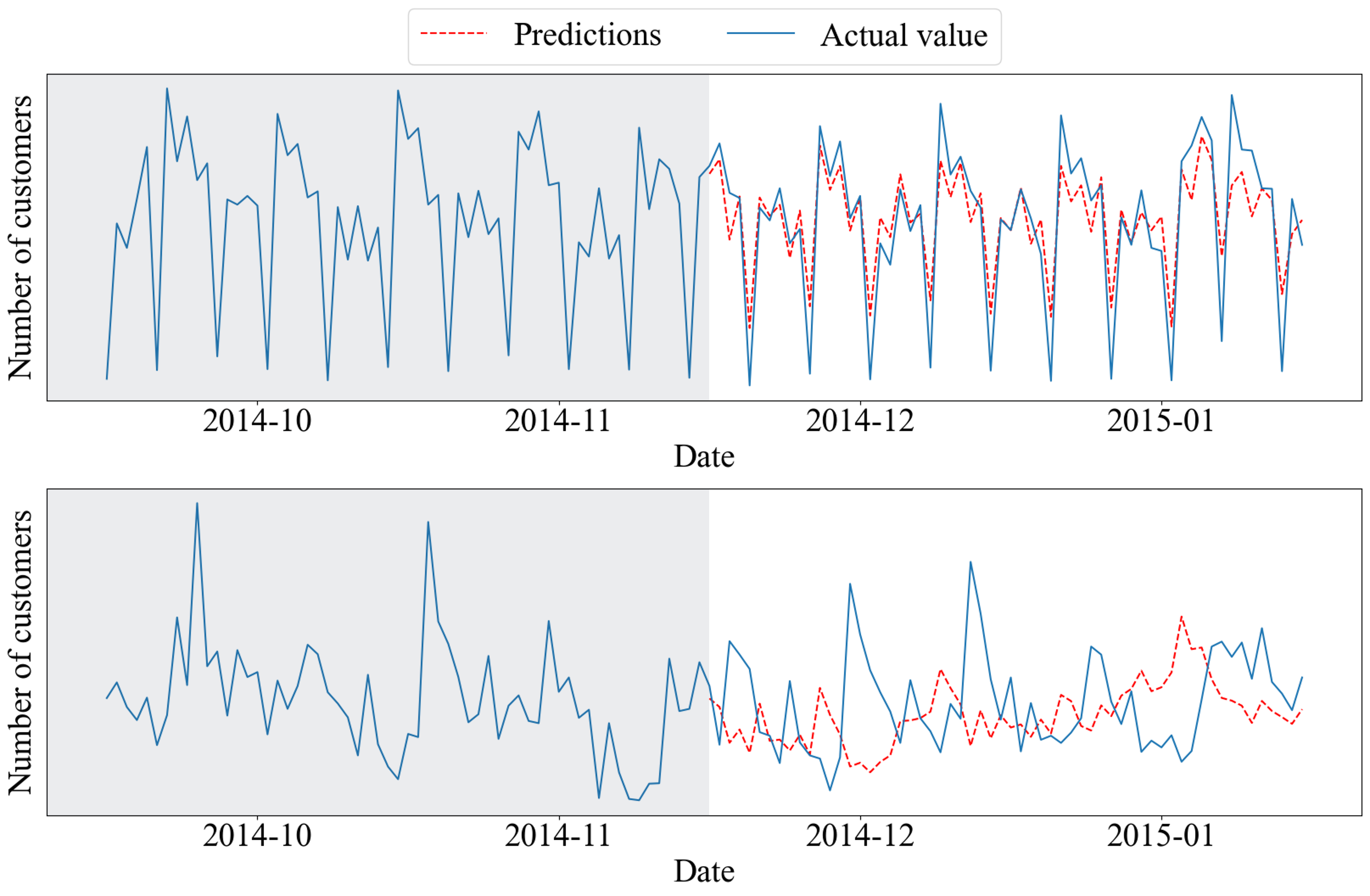
Figure 1. Daily number of customers (in blue), from September 2014 to January 2015, at two different stores in the Rossmann drug store chain. Predictions (in red), starting November 2014, are generated using Exponential Smoothing with the same fitting process. The store in the upper sub-figure has substantially more accurate predictions ($R^{2}=0.88$) than that of the lower sub-figure ($R^{2}=0.11$).

To summarize so far, the repeated newsvendor with unknown, nonstationary demand (which from here on we refer to as the Nonstationary Newsvendor) admits policies with nontrivial guarantees, which can be made significantly better or worse by following predictions. This suggests the opportunity to design a policy that leverages predictions optimally, in the sense that the predictions are utilized when accurate, and ignored when inaccurate. Ideally, such a policy should operate without knowledge of (a) the accuracy of the predictions and (b) the method with which they are generated. This is precisely what we accomplish in this paper.

1.1. The Nonstationary Newsvendor, with and without Predictions

The primary purpose of this paper is to develop a policy that optimally incorporates predictions (defined in the most generic sense possible) into the Nonstationary Newsvendor problem. Naturally, a prerequisite to this is a fully-solved model of the Nonstationary Newsvendor without predictions. At present this prerequisite is only partially satisfied (via the work of [6]), so a nontrivial portion of our contributions will be to fully solve this problem.

Without predictions, the Nonstationary Newsvendor consists of a sequence of newsvendor problems indexed by periods $t\in 1,\ldots,T$, each with unknown demand distribution $D_{t}$. The level of nonstationarity is characterized via a variation parameter $v\in[0,1]$, where $v=0$ essentially amounts to stationary demand, and $v=1$ is effectively arbitrary (in a little more detail: a deterministic analogue of quadratic variation is applied to the sequence of means $\{\mathbb{E}[D_{1}],\ldots,\mathbb{E}[D_{T}]\}$, and $v\in[0,1]$ is the exponent such that this quantity equals $T^{v}$). Finally, we measure the performance of any policy using regret, which is the expected difference in the total cost incurred by the policy versus that of an optimal policy that “knows” the demand distributions. At minimum we aim to design a policy that achieves sub-linear (i.e. $o(T)$) regret, as such a policy would incur a per-period cost that is on average no worse than the optimal, as $T$ grows. We will in fact design policies which achieve order-optimal regret with respect to the variation parameter $v$.

To this base problem, we introduce the notion of predictions. In each period we receive a prediction $a_{t}$ of the mean demand $\mu_{t}=\mathbb{E}[D_{t}]$ before selecting the order quantity. Our predictions are generic: no assumption is made on how they are generated. We measure the accuracy of the predictions through an accuracy parameter $a\in[0,1]$, defined such that $\sum_{t=1}^{T}|a_{t}-\mu_{t}|=T^{a}$. Notice that when $a=0$ the predictions are almost perfect, and when $a=1$ the predictions are effectively useless. We will characterize a precise threshold on $a$ (which depends on $v$) that determines when the predictions should be utilized. Our primary challenge will be to design a policy that makes use of the predictions only when they are sufficiently accurate, and without having access to $a$. As to the variation parameter $v$, we will separately consider policies which do and do not have access to $v$ – this distinction will turn out to be the critical factor in classifying what is and is not achievable.

1.2. Our Contributions

Our primary contributions can be summarized as follows.

1. Nonstationary Newsvendor (without predictions): We completely solve the Nonstationary Newsvendor problem. This consists of first constructing a policy and proving an upper bound on its regret:

Theorem 1.1 (Informal).

There exists a policy which achieves $\tilde{O}(T^{(3+v)/4})$ regret without knowing $v$.

We then show that this regret is minimax optimal up to logarithmic factors:

Proposition 1.1 (Informal).

No policy can achieve regret better than $O(T^{(3+v)/4})$, even if $v$ is known.

As alluded to earlier, [6] previously initiated the study of the Nonstationary Newsvendor. Our results are distinct in terms of both modeling and theoretical contributions.

• Modeling: The most crucial difference in our model is that we allow both the demand and the set of possible ordering quantities to be discrete. This is undoubtedly of practical concern (e.g. physical inventory, employees, and virtual machines are all indivisible units of demand), but moreover, we will show that the results of [6] require both the demand and set of feasible ordering quantities to be continuous. Thus, there is no overlap in our theoretical results.

• Results: [6] succeed in designing a policy that achieves order-optimal regret, but crucially, their policy requires that the variation parameter $v$ be known. In addition to being concerning from a practical standpoint, this leaves open the theoretical question of what exactly is achievable in settings for which $v$ is unknown. Our results show that the same regret can be achieved without knowing $v$.

We will expound these distinctions more carefully later on.

2. Nonstationary Newsvendor with Predictions:

We construct a policy that optimally leverages predictions, i.e. it is robust to unknown prediction accuracy. To be precise, the previous contribution offers a policy that achieves $\tilde{O}(T^{(3+v)/4})$ regret, and predictions yield a simple policy that achieves $O(T^{a})$ regret, so we would expect that the best possible regret is the minimum of these two quantities. We show this formally:

Proposition 1.2 (Informal).

No policy can achieve regret better than $O(T^{\min\{(3+v)/4,a\}})$, even if $v$ and $a$ are known.

Our main algorithmic contribution is a policy which achieves this lower bound (up to log factors) without knowing the prediction accuracy:

Theorem 1.2 (Informal).

There exists a policy which achieves regret $\tilde{O}(T^{\min\{(3+v)/4,a\}})$, knowing $v$, and without knowing $a$.

Finally, since our policy relies on knowledge of the variation parameter $v$, the remaining question is whether or not the same regret is achievable if both $v$ and $a$ are unknown. We show that in fact predictions cannot be incorporated in any meaningful way when this is the case:

Proposition 1.3 (Informal).

If $v$ and $a$ are unknown, then no policy can achieve regret better than $O(T^{\max\{(3+v)/4,a\}})$ for all $v,a\in[0,1]$.

Our theoretical results are summarized in Table 1. Each entry has a corresponding policy that achieves the stated regret, along with a matching lower bound.

	Without predictions	With predictions of unknown accuracy
Known variation	$\qquad\tilde{O}(T^{(3+v)/4})$	$\tilde{O}(T^{\min\{(3+v)/4,a\}})$
Unknown variation	$\tilde{O}(T^{(3+v)/4})$	$\tilde{O}(T^{\max\{(3+v)/4,a\}})$

Table 1. Summary of Main Theoretical Results. Each entry has a corresponding policy that achieves the stated regret, along with a matching lower bound.

3. Empirical Results: Finally, we demonstrate the practical value of our model (namely the Nonstationary Newsvendor with Predictions) and our policy via empirical results on two real-world datasets corresponding to our two motivating applications above: daily web traffic for Wikipedia.com (of various languages) and daily foot traffic across the Rossmann store chain. These datasets together contain over one thousand individual time-series on which we generate predictions of varying quality, using four different popular forecasting and machine learning algorithms. We apply our policy, and compare its performance against the two most-natural baseline policies: our optimal policy without predictions, and the simple policy which always utilizes the predictions (these correspond to the two “existing approaches” described previously). On any given experimental instance (i.e. a time-series and a set of predictions), the minimum (maximum) of the costs incurred by these two baselines can be viewed as the best (worst) we can hope for. Thus we measure performance in terms of the proportion of the gap between these two costs incurred by our policy, so if this “optimality gap” is close to 0, our policy performs almost as good as the better one of the two baselines.

We find that in the Rossmann dataset, the average optimality gap is 0.26 when the predictions are accurate, and 0.28 when the predictions are inaccurate. In the Wikipedia dataset, the average optimality gap is 0.40 when the predictions are accurate, and 0.07 when the predictions are inaccurate. This demonstrates that our policy performs well, irrespective of the quality of the predictions.

The remainder of this paper is organized as follows. The current section concludes with a literature review. In Section 2 we introduce our model of the Nonstationary Newsvendor (without predictions), and then present matching upper and lower regret bounds in Section 3. We then introduce predictions to our model in Section 4, and again offer matching regret bounds. Section 5 contains our experimental results, and Section 6 concludes the paper.

1.3. Literature Review

The earliest works on the newsvendor model assume that the demand distribution is fully known [9, 10]. This assumption has then been relaxed, and we can divide the approaches in which the demand distribution is unknown into parametric and nonparametric ones. One of the most popular parametric approaches is the Bayesian approach, where there is a prior belief in parameters of the demand distribution, and such belief is updated based on observations that are collected over time. [11] first applied the Bayesian approach to inventory models, and later this is studied in many works [14, 15, 13, 12]. [16] introduced another parametric approach called operational statistics which, unlike the Bayesian approach, does not assume any prior knowledge on the parameter values. Instead it uses past demand observations to directly estimate the optimal ordering quantity.

Nonparametric approaches have been developed in recent years. The first example of a nonparametric approach is the SAA method, first proposed by [20] and [21]. [22] applied SAA to the newsvendor problem by using samples to approximate the optimal ordering quantity, and [7] improve significantly upon the bounds of [22] for the same problem. Other non-parametric approaches include stochastic gradient descent algorithms [23, 24, 17] and the concave adaptive value estimation (CAVE) method [25, 26]. With the development of machine learning, [18] and [19] propose machine learning/deep learning algorithms using demand features and historical data to solve the newsvendor problem.

All the previous studies consider the newsvendor in a static environment where the demand distribution is the same over time. However, in reality the demand distribution is often nonstationary. There are two common practices to resolve this issue. The first is to model the nonstationarity and utilize past demand observations according to the model. One common way is to model the nonstationarity as a Markov chain. For example, [28] applied this idea to inventory management and [29] and [30] applied this idea to revenue management. Another approach is to bound the nonstationarity via a variation budget, which has been applied to stochastic optimization [32], dynamic pricing [27], multi-armed bandit [31], newsvendor problem [6], etc. As mentioned before, [6] is particularly relevant, so we delay a careful comparison to Sections 2 and 3

The second common practice is to use predictions on the demand distribution of each time period. Predictions can often be obtained e.g. via machine learning, and a recent line of work looks to help decision-making by incorporating predictions. This framework has been applied to many online optimization problems such as revenue optimization [34, 33], caching [35, 36], online scheduling [37], and the secretary problem [8]. In this paper we will combine the nonstationarity framework and the prediction framework on the newsvendor problem.

2. Model: The Nonstationary Newsvendor (without Predictions)

We begin this section with a formal description of the Nonstationary Newsvendor, along with a comparison to the problem of the same name from [6]. Consider a sequence of newsvendor problems over $T$ time periods labeled $t=1,\dots,T$. At the beginning of each time period $t$, the decision-maker selects a quantity $q_{t}\in Q$, where $Q$ is a fixed, bounded subset of $\mathbb{R}$. Then the period’s demand $d_{t}$ is drawn from an (unknown) demand distribution $D_{t}$, which depends on the time period $t$. Finally a cost is incurred – specifically, there is a (known) per-unit underage cost $b_{t}\in[0,b_{\max}]$ and a (known) per-unit overage cost $h_{t}\in[0,h_{\max}]$, so that the total cost is equal to

$$b_{t}(d_{t}-q_{t})^{+}+h_{t}(q_{t}-d_{t})^{+},$$

where $x^{+}=\max\{0,x\}$. The decision-maker observes the realized demand $d_{t}$, and thus the cost.

Note that requiring $q_{t}\in Q$ does not impose any restriction on modeling, since $Q$ could simply be selected to be $\mathbb{R}$ (as in much of the literature). In fact, introducing $Q$ allows for modeling important practical concerns such as batched invnetory or even simply the integrality of physical items. As we will discuss momentarily, this is a non-trivial concern insofar as theoretical guarantees are concerned.

To complete our description of the Nonstationary Newsvendor, we will need to (a) impose a few assumptions on the demand distributions, and then (b) describe how “nonstationarity” is quantified. These are, respectively, the subjects of the following two subsections.

2.1. Demand Distributions

We will assume that the demand distributions come from a known, parameterized family of distributions $\mathcal{D}$:

Assumption 2.1.

Every demand distribution $D_{t}$ comes from a family of distributions $\mathcal{D}$ satisfying the following:

• $\mathcal{D}=\{\mathcal{D}_{\mu}:\mu\in[\mu_{\min},\mu_{\max}]\}$, that is $\mathcal{D}$ is parameterized by a scalar $\mu$ taking values in some bounded interval.

• Each distribution $\mathcal{D}_{\mu}\in\mathcal{D}$ is sub-Gaussian with $O(1)$ sub-Gaussian norm.

Assumption 2.1 is fairly minimal. Parsing it in reverse: the sub-Gaussianity in part (b) allows for many commonly-used variables, such as the Gaussian distribution and any bounded random variable, while letting us eventually apply Hoeffding-type concentration bounds. Part (a) is particularly minimal at the moment, as $\mu$ represents an arbitrary parameterization of $\mathcal{D}$, but will become meaningful when combined with Assumption 2.2. The choice of the symbol “$\mu$” might suggest that $\mu$ represents the mean of $\mathcal{D}_{\mu}$, and indeed this is what we will assume from here on. But it should be emphasized that our taking $\mu=\mathbb{E}[\mathcal{D}_{\mu}]$ is strictly for notational convenience (because we will frequently need to refer to the means of these distributions): if $\mu$ were any other parameterization of $\mathcal{D}$, we could simply define a mapping from $\mu$ to the mean values.

Now define $C(\mu,b,h,q)$ to be the expected newsvendor cost when selecting quantity $q\in Q$, given underage/overage costs $b$ and $h$, and demand distribution $\mathcal{D}_{\mu}$:

$$C(\mu,b,h,q)=\mathbb{E}_{\mathcal{D}_{\mu}}[b(\mathcal{D}_{\mu}-q)^{+}+h(q-\mathcal{D}_{\mu})^{+}].$$

The critical assumption, with respect to the parameterization in Assumption 2.1(a), is that the expected cost is well-behaved as a function of $\mu$:

Assumption 2.2.

For every $b\in[0,b_{\max}]$, $h\in[0,h_{\max}]$, and $q\in Q$, the function $C(\cdot,b,h,q)$ is Lipschitz on its domain $[\mu_{\min},\mu_{\max}]$, i.e. there exists $\ell\in\mathbb{R}^{+}$ such that for every $\mu_{1},\mu_{2}\in[\mu_{\min},\mu_{\max}]$, we have

$$|C(\mu_{1},b,h,q)-C(\mu_{2},b,h,q)|\leq\ell|\mu_{1}-\mu_{2}|.$$

Note that in the above description, the Lipschitz constant $\ell$ may depend on $b,h,$ and $q$, but by continuity, there exists a single $\ell$ so that the above holds for all $b,h,q$ simultaneously.

Some useful examples of families $\mathcal{D}$ satisfying Assumptions 2.1 and 2.2 are the following:

1. $\mathcal{D}_{\mu}\sim\mathcal{N}(\mu,\sigma^{2})$, i.e. the family of normal distributions with fixed variance $\sigma^{2}$. In this case, $\ell=O(\sigma(b_{\max}+h_{\max}))$. As a generalization of this, the variances $\sigma^{2}$ vary (continuously) with $\mu$.

2. $\mathcal{D}_{\mu}=\mu+\epsilon$, where $\epsilon$ is any mean-zero, sub-Gaussian variable.

3. The Poisson distribution is frequently used to model demand (since arrivals are often modeled as a Poisson process). While the Poisson distribution is not sub-Gaussian, any reasonable truncation satisfies our assumptions. For example, $\mathcal{D}_{\mu}\sim\min\{\mathrm{Poisson}(\mu),K\mu\}$, for some constant $K$. Here, $K$ can be taken to be large enough so that the truncation happens with small probability (in fact, this probability is $O(e^{-K\mu})$).

To understand the reasoning behind Assumption 2.2, consider the problem faced at some time $t$. The optimal choice for the decision-maker here is

(2.1) $$q_{t}^{*}\in\text{argmin}_{q\in Q}C_{t}(\mu_{t},q),$$

where $\mu_{t}$ is the mean of $D_{t}$ (i.e. $D_{t}\sim\mathcal{D}_{\mu_{t}}$), and $C_{t}(\mu,q)=C(\mu,b_{t},h_{t},q)$ to simplify the notation. Since $D_{t}$ is unknown, it is likely that some $q_{t}\neq q_{t}^{*}$ will ultimately be selected, and we could measure the sub-optimality of this decision (i.e. regret, to be defined soon): $C_{t}(\mu_{t},q_{t})-C_{t}(\mu_{t},q_{t}^{*})$. It would be natural then to try to characterize this suboptimality as a function of $|q_{t}-q_{t}^{*}|$, but in fact all of the algorithms we will consider “work” by making an estimate $\hat{\mu}_{t}$ of $\mu_{t}$, and then selecting $\hat{q}_{t}\in\text{argmin}_{q\in Q}C_{t}(\hat{\mu}_{t},q)$. So motivated, the purpose of Assumption 2.2 is to allow us to “translate” error in our estimate of $\mu_{t}$ to (excess) costs. The following structural lemma makes this precise, and will be used throughout the paper.

Lemma 2.1.

Fix any $b$ and $h$ (we will suppress them from the notation). For any $D_{\mu_{1}},D_{\mu_{2}}\in\mathcal{D}$, let $q_{1}^{*}\in\text{argmin}_{q\in Q}C(\mu_{1},q)$ and $q_{2}^{*}\in\text{argmin}_{q\in Q}C(\mu_{2},q)$. Then we have

$$C(\mu_{1},q_{2}^{*})-C(\mu_{1},q_{1}^{*})\leq 2\ell|\mu_{1}-\mu_{2}|.$$

Proof.

By Assumption 2.2, we have

$$C(\mu_{1},q_{2}^{*})-C(\mu_{1},q_{1}^{*}) = C(\mu_{1},q_{2}^{*})-C(\mu_{2},q_{1}^{*})+C(\mu_{2},q_{1}^{*})-C(\mu_{1},q_{1}^{*})$$

$$\overset{(a)}{\leq} C(\mu_{1},q_{2}^{*})-C(\mu_{2},q_{1}^{*})+\ell|\mu_{1}-\mu_{2}|$$

$$\overset{(b)}{\leq} C(\mu_{1},q_{2}^{*})-C(\mu_{2},q_{2}^{*})+\ell|\mu_{1}-\mu_{2}|$$

$$\overset{(c)}{\leq} 2\ell|\mu_{1}-\mu_{2}|.$$

Here $(a)$ and $(c)$ follow from $C(\mu,q)$ being $\ell$-Lipchitz in $\mu$, and $(b)$ follows by the definition of $q_{2}^{*}$. ∎

In words, Lemma 2.1 states that estimation error of the mean $\mu_{t}$ translates linearly to excess cost.

(Optional) Aside: Comparison to [6]: The final component in describing the Nonstationary Newsvendor is defining a proper quantification of nonstationarity. Before we do so, this is the proper location to delineate the modeling differences between our Nonstationary Newsvendor and that of [6]. There are two primary differences:

1. Our set of allowed order quantities $Q$ is bounded, but otherwise arbitrary. In particular, it need not contain the optimal unconstrained order quantity $\text{argmin}_{q\in\mathbb{R}}C(\mu,q)$ for each $\mu$ (or any $\mu$, for that matter). [6] assume $Q=\mathbb{R}^{+}$.

2. The demand distributions in [6] are assumed to be continuous. We make no such restriction.

Besides the practical reasons why discrete quantites arise in practice (non-divisible items, batched inventory, etc.), the primary consequence of either of the two differences above is that they preclude a critical lemma used in [6] (and in fact by [22]) which states that $C(\mu_{1},q_{2}^{*})-C(\mu_{1},q_{1}^{*})$ (as defined in our Lemma 2.1) scales as $(q_{1}^{*}-q_{2}^{*})^{2}$. This scaling does not necessarily hold when either $Q$ or the demand distribution is discrete.

2.2. Demand Variation

Just as in [6] (and [27] before that), we measure the level of nonstationarity via a deterministic analogue of quadratic variation for the sequence of means $\mu_{1},\ldots,\mu_{T}$. Specifically, define a partition of the time horizon $\{1,\dots,T\}$ to be any subset of time periods $\{t_{0},\dots,t_{K}\}$ where $1\leq t_{0}<\cdots<t_{K}\leq T$. Then for any sequence of means $\bm{\mu}=\{\mu_{1},\dots,\mu_{T}\}$, its demand variation is

$$V_{\bm{\mu}}=\max_{\{t_{0},\dots,t_{K}\}\in\mathcal{P}}\left\{\sum_{k=1}^{K}\left(\mu_{t_{k}}-\mu_{t_{k-1}}\right)^{2}\right\},$$

where $\mathcal{P}$ is the set of all partitions.

To motivate the use of partitions in the definition of $V_{\bm{\mu}}$, it is worth contrasting with a measure that may feel more natural, namely the sum of squared differences (SSD) between consecutive terms, $\sum_{t=2}^{T}\left(\mu_{t}-\mu_{t-1}\right)^{2}$, which corresponds to taking the densest possible partition $\{1,2,\ldots,T\}$. The maximum in the definition of $V_{\bm{\mu}}$ is not necessarily achieved by selecting the densest possible partition, but rather by setting $t_{0},\dots,t_{K}$ to be the periods when the sequence $\mu_{1},\dots,\mu_{T}$ changes direction. Thus, the demand variation penalizes trends, or consecutive increases/decreases, more so than the SSD. For example, the mean sequences $\bm{\mu_{1}}=\{1,2,3,4,5\}$ and $\bm{\mu_{2}}=\{1,0,1,0,1\}$, respective variations $V_{\bm{\mu_{1}}}=(5-1)^{2}=16$ and $V_{\bm{\mu_{2}}}=1^{2}+1^{2}+1^{2}+1^{2}+1^{2}=5$, despite having identical SSDs.

All of our theoretical guarantees (upper and lower bounds) will be parameterized by $V_{\bm{\mu}}$. This quantity of course depends on $T$, and so it is natural to allow $V_{\bm{\mu}}$ to grow $T$. It will turn out that the most natural parameterization of this growth is via what we will simply call the variation parameter $v\in[0,1]$, such that $V_{\bm{\mu}}=BT^{v}$, where $B$ is some constant (which we take to be equal to one from here on). We denote the set of demand distribution sequences $\{D_{1},\dots D_{T}\}$ whose means $\bm{\mu}=\{\mu_{1},\dots,\mu_{T}\}$ satisfy $V_{\bm{\mu}}\leq T^{v}$ as

$$\mathcal{D}(v)=\{\{D_{1},\dots D_{T}\}:D_{t}\in\mathcal{D}\text{ for all }t\text{ and }V_{\bm{\mu}}\leq T^{v}\}.$$

In the next section, we will show via a minimax lower bound that non-trivial guarantees are only achievable when $v<1$, and provide an algorithm which achieves the same bound.

Aside: Time-Series Modeling: At this point, we have fully described our model for the Nonstationary Newsvendor. All that remains is to define our performance metric, which we will do in the next subsection. We conclude this subsection with an important practical consideration with respect to time-series models and our variation parameter.

Consider, as an example, the following class of time-series models:

(2.2) $$d_{t}=R(t)+S(t)+\epsilon_{t}.$$

Here, $R(t)$ represents a deterministic (and usually simple, e.g. linear) function representing some notion of “trend,” and $S(t)$ represents a deterministic, period function representing some notion of “seasonality.” Finally, all stochastic behavior is captured by the random variables $\epsilon_{t}$, which are assumed to be independent and mean-zero. This time-series model is classic, and yet drives simple forecasting algorithms (e.g. exponential smoothing) which are still competitive in modern forecasting competitions [3].

The above model raises an important practical issue: if there exists any (non-trivial) trend $R(\cdot)$ or seasonality $S(\cdot)$, then the demand variation of the sequence of means $\mu_{t}=R(t)+S(t)$ would scale at least as $T$, meaning $v=1$ and no meaningful guarantee will be achievable. Our main observation is that time-series effects like trend and seasonality are easily detected and estimated, so that in any practical setting, estimates $\hat{R}(\cdot)$ and $\hat{S}(\cdot)$ should be available, and used to de-trend and de-seasonalize the data. Concretely, the Nonstationary Newsvendor would take place on the sequence

$$\tilde{d_{t}}=d(t)-\hat{R}(t)-\hat{S}(t)=(R(t)-\hat{R}(t))+(S(t)-\hat{S}(t))+\epsilon_{t}.$$

The resulting sequence of means $\mu_{t}=(R(t)-\hat{R}(t))+(S(t)-\hat{S}(t))$ does not stem from the trend and seasonality, but rather the error in estimating the trend and seasonality. It is precisely this error that is assumed to be nonstationary, but with reasonable variation parameter.

2.3. Performance Metric: Regret

We conclude this section by formally defining our performance metric for any policy. A policy is simply a sequence of mappings $\pi=\{\pi_{1},\dots,\pi_{T}\}$, where each $\pi_{t}$ is a mapping from $d_{1},\dots,d_{t-1}$ to an order quantity $q_{t}\in Q$ at time $t$ (by convention, $\pi_{1}$ is a constant function).

We measure the performance of policy by its regret. Fix a sequence of demand distributions $\bm{D}=\{D_{1},\dots,D_{T}$}. Following the earlier notation from (2.1), the regret incurred by a policy which selects order quantities $q_{1},\ldots,q_{T}$ is

$$\mathbb{E}^{\pi}_{\bm{D}}\left[\sum_{t=1}^{T}\left(C_{t}(\mu_{t},q_{t})-C_{t}(\mu_{t},q^{*}_{t})\right)\right],$$

where the expectation is with respect to the randomness of the realized demands. In words, the regret measures the difference between the (expected) total cost incurred by the policy and that of a clairvoyant that knows the underlying demand distributions $\bm{D}=\{D_{1},\dots,D_{T}$}.

We will be concerned with the worst-case regret of a policy across families of instances (i.e. sequences of demand distributions) controlled by the variation parameter $v$:

$$\mathcal{R}^{\pi}(T)=\sup_{\bm{D}\in\mathcal{D}(v)}\mathbb{E}^{\pi}_{\bm{D}}\left[\sum_{t=1}^{T}\left(C_{t}(\mu_{t},q_{t})-C_{t}(\mu_{t},q^{*}_{t})\right)\right].$$

Note that if the worst-case regret $\mathcal{R}^{\pi}(T)$ of some policy is sublinear in $T$, then that policy is essentially cost-optimal on average as $T$ goes to infinity. In the next section, we will prove a lower bound on the achievable across all policies, and describe an algorithm which achieves this lower bound.

3. Solution to the Nonstationary Newsvendor (without Predictions)

This section contains a complete solution (i.e. matching lower and upper bounds on regret) to the Nonstationary Newsvendor. We begin with the lower bound:

Proposition 3.1 (Lower Bound: Nonstationary Newsvendor).

For any variation parameter $v\in[0,1]$, and any policy $\pi$ (which may depend on $v$), we have

$$\mathcal{R}^{\pi}(T)\geq cT^{(3+v)/4},$$

where $c>0$ is a universal constant.

The above result is a corollary of a more general lower bound in Proposition 4.1, which will be given in the next section, and so the proof is omitted. Indeed, it will turn out the Nonstationary Newsvendor is itself a special case of the Nonstationary Newsvendor with Predictions.

Proposition 3.1 states that the regret of any policy is at least $\Omega(T^{(3+v)/4})$. It is useful to contrast this with two existing results:

1. [38] showed that, for a completely stationary newsvendor (i.e. identical demand distributions at every time period), there exists a policy that achieves a worse-case regret of $O(\log T)$. This might appear to be incompatible with our result, which states a lower bound of $\Omega(T^{3/4})$ when $v=0$, but in fact the case of $v=0$ is more general than i.i.d. demand. For example, a demand sequence can have $O(\log T)$ changes in the mean, and its variation parameter would still be $0$.

2. [6] showed that, a lower bound of $\Omega(T^{(2+v)/3})$ for their version of the nonstationary newsvendor. This is strictly lower than our lower bound, and as we described in Section 2.1, comes from a stronger (quadratic) relationship between error and regret that requires stronger modeling assumptions.

In the next two subsections, we will first analyze a simple algorithm which achieves the lower bound of Proposition 3.1 when the variation parameter $v$ is known, and then use this as a building block for an algorithm which again achieves the same bound when $v$ is unknown.

3.1. Upper Bound with Known Variation Parameter $v$

If we assume that $v$ is known, then designing a policy which achieves a worst-case regret matching Proposition 3.1 is fairly straightforward. In fact, a simple policy based on averaging a fixed number of past demand observations does the job ([6] use the same policy). That policy, which we call the Fixed-Time-Window Policy is defined in Algorithm 1.

Inputs: variation parameter $v\in[0,1]$ and scaling constant $\kappa>0$

Initialization: $n\leftarrow\lceil\kappa T^{(1-v)/2}\rceil$

for $t=1,\ldots,n$ do

       select $q_{t}\in Q$ arbitrarily;

for $t=n+1,\ldots,T$ do

       $\hat{\mu}_{t}\leftarrow\frac{1}{n}\sum_{s=t-n}^{t-1}d_{s}$ (if $\hat{\mu}_{t}\notin[\mu_{\min},\mu_{\max}]$, round $\hat{\mu}_{t}$ to the nearest value in $[\mu_{\min},\mu_{\max}]$);

       $q_{t}\leftarrow\text{argmin}_{q\in Q}C_{t}(\hat{\mu}_{t},q)$;

      

Algorithm 1 Fixed-Time-Window Policy

The Fixed-Time-Window Policy uses a carefully-selected “window” size $n$ that is on the order of $T^{(1-v)/2}$. At each time period $t$, it constructs an estimate $\hat{\mu}_{t}$ of the mean by averaging the observed demands from the previous $n$ periods, and then selects the optimal order quantity corresponding to $\hat{\mu}_{t}$. Note that Algorithm 1 also includes a “scaling constant” $\kappa$ – this should be thought of as a practical tuning parameter, but for the coming theoretical result, it can be chosen arbitrarily (e.g. $\kappa=1$ suffices).

The worst-case regret of the Fixed-Time-Window Policy is upper bounded in the following result:

Lemma 3.1 (Upper Bound: Nonstationary Newsvendor with Known $v$).

Fix any variation parameter $v\in[0,1]$. The Fixed-Time-Window Policy $\pi^{\mathrm{fixed}}$ achieves worst-case regret

$$\mathcal{R}^{\pi^{\mathrm{fixed}}}(T)\leq CT^{(3+v)/4},$$

where $C$ is a universal constant.

As promised, Lemma 3.1 shows that the Fixed-Time-Window Policy achieves regret that matches the lower bound in Proposition 3.1. Its proof can be found in Appendix B, and amounts to bounding the estimation error incurred by demand noise (which is worse for smaller time windows) and demand mean variation (which is worse for larger time windows). The carefully-chosen time window used in the policy comes from balancing these two sources of error.

3.2. Upper Bound with Unknown Variation Parameter $v$

The lower regret bound in Proposition 3.1 holds for policies that “know” $v$. Naturally, it also holds for policies that do not know $v$, but an unanswered question at the moment is whether (a) the lower bound should be even larger when $v$ is unknown, or (b) there exists a policy that matches Proposition 3.1 without knowing $v$. We show here that case (b) holds by constructing such a policy. Our policy uses time windows in the same way as the previous Fixed-Time-Window Policy, but the length of the time window itself changes (decreases, specifically) over time. We call this the Shrinking-Time-Window Policy (Algorithm 2).

Inputs: scaling constants $\kappa>0$, and $\gamma$ sufficiently large (Equations C.2 in Appendix C);

Initialization: Set $\mathcal{V}=\{v_{1},\ldots,v_{k}\}$ and $\{n_{1},\ldots,n_{k}\}$ according to Equations LABEL:eqn:vi,eqn:ni;

for $t=1,\ldots,T^{3/4}$ do

       select $q_{t}\in Q$ arbitrarily;

Initialize $i\leftarrow 1$ and $t_{\textbf{if}}\leftarrow T^{3/4}+1$;

for $t=T^{3/4}+1,\ldots,T$ do

       if $\sum_{s=t_{\emph{{if}}}}^{t}|\hat{\mu}_{s}^{i}-\hat{\mu}_{s}^{j}|\geq 2\left(\gamma\sqrt{\log T}+\sqrt{\kappa}\right)T^{(3+v_{j})/4}$ for some $j>i$ then

             $i\leftarrow i+1$;

             $t_{\textbf{if}}\leftarrow t$;

            

       $q_{t}\leftarrow\text{argmin}_{q\in Q}C_{t}(\hat{\mu}_{t}^{i},q)$;

      

Algorithm 2 Shrinking-Time-Window Policy

To begin, a discrete set of candidate variation parameters $\mathcal{V}=\{v_{1},\ldots,v_{k}\}$, and corresponding time windows $\{n_{1},\ldots,n_{k}\}$, are defined:

(3.1) $$v_{i} =\left(1+\frac{1}{\log T}\right)^{i-1}\frac{1}{\log T},\quad i=1,\ldots,k$$

(3.2) $$n_{i} =\lceil\kappa T^{(1-v_{i})/2}\rceil,$$

where $\kappa>0$ is again an arbitrary scaling constant, and $k$ is chosen precisely so that $v_{k-1}<1\leq v_{k}$. At any given period $t$, the policy behaves as if the variation parameter is some $v_{i}\in\mathcal{V}$, and thus estimates $\mu_{t}$ using the same fixed time window estimator:

(3.3) $$\hat{\mu}_{t}^{i}=\frac{1}{n_{i}}\sum_{s=t-n_{i}}^{t-1}d_{s},\quad\text{rounded to the nearest value in }[\mu_{\min},\mu_{\max}].$$

Finally, the index $i$ is initially taken to be $1$ (corresponding to the smallest variation parameter, and thus the largest window size), and increments at any period in which the policy observes a carefully-designed “certificate” that the current window size is too large $n_{i}$.

This policy’s worst-case regret matches (up to log factors) the lower bound in Proposition 3.1:

Theorem 3.1 (Upper Bound: Nonstationary Newsvendor with Unknown $v$).

For any variation parameter $v\in[0,1]$, the Shrinking-Time-Window Policy $\pi^{\mathrm{shrinking}}$ achieves worst-case regret

$$\mathcal{R}^{\pi^{\mathrm{shrinking}}}(T)\leq CT^{(3+v)/4}\log^{5/2}T,$$

where $C$ is a universal constant.

The proof of Theorem 3.1 can be found in Appendix C. At a high level, the proof works as follows:

Proof Sketch of Theorem 3.1.

First note that the total regret incurred during the first $T^{3/4}$ time periods is at most $O(T^{3/4})$. After that, the total regret incurred during the time periods in which the if condition in Algorithm 2 is triggered is at most $O(k)$, where $k$ is the number of candidate variation parameters defined in eq. 3.1, and $k\approx\log^{2}T$. Thus, it suffices to bound the total regret incurred between successive triggerings of the if condition. As a final reduction before proceeding, consider the smallest candidate variation parameter that is at least $v$, i.e. define $\ell$ to be the smallest index such that $v\leq v_{\ell}$. Because $v_{\ell}=\left(1+\frac{1}{\log T}\right)v_{\ell-1}$, we have that $T^{v_{\ell}}$ is a constant multiple away from $T^{v}$. Thus, it will suffice to bound the total regret by $O(T^{(3+v_{\ell})/4}\log^{5/2}T)$.

To do this, we first show that (with high probability) throughout the algorithm, the running index $i$ never exceeds $\ell$. To see this, consider the following steps:

1. For every $j\geq\ell$, because $v\leq v_{j}$, by Lemma 3.1 the Fixed-Time-Window Policy corresponding to the window size $n_{j}$ has worst-case regret $O(T^{(3+v_{j})/4})$. In addition, we can show with high probability (via Hoeffding’s inequality) that $\sum_{s=n_{j}+1}^{T}|\hat{\mu}_{s}^{j}-\mu_{s}|\leq\left(\gamma\sqrt{\log T}+\sqrt{\kappa}\right)T^{(3+v_{j})/4}$ for every $j\geq\ell$. We may assume this event occurs from now on.

2. For the sake of contradiction, suppose $i$ exceeds $\ell$ at some period $t$, or equivalently, there is a period $t$ in which $i\geq\ell$, and the if condition is triggered with some $j>i$. Then we have

   $$\sum_{s=t_{\textbf{if}}}^{t}|\hat{\mu}_{s}^{i}-\hat{\mu}_{s}^{j}| \overset{(a)}{\leq}\sum_{s=t_{\textbf{if}}}^{t}|\hat{\mu}_{s}^{i}-\mu_{s}|+\sum_{s=t_{\textbf{if}}}^{t}|\hat{\mu}_{s}^{j}-\mu_{s}|$$

   $$\overset{(b)}{\leq}\sum_{s=n_{i}+1}^{T}|\hat{\mu}_{s}^{i}-\mu_{s}|+\sum_{s=n_{j}+1}^{T}|\hat{\mu}_{s}^{j}-\mu_{s}|$$

   $$\overset{(c)}{\leq}\left(\gamma\sqrt{\log T}+\sqrt{\kappa}\right)\cdot T^{(3+v_{i})/4}+\left(\gamma\sqrt{\log T}+\sqrt{\kappa}\right)\cdot T^{(3+v_{j})/4}$$

   $$\overset{(d)}{<}2\left(\gamma\sqrt{\log T}+\sqrt{\kappa}\right)\cdot T^{(3+v_{j})/4},$$

   where $(a)$ is the triangle inequality and $(b)$ holds because $t_{\textbf{if}}>T^{3/4}$ and $n_{i},n_{j}\leq\kappa T^{1/2}$; since $j>i\geq\ell$, by our assumption in the previous step we get $(c)$; $(d)$ follows since $v_{j}>v_{i}$. But this directly contradicts our assumption that the if condition is triggered at period $t$. Therefore $i$ never exceeds $\ell$.

Now suppose two consecutive if conditions occur at times $t^{\prime}$ and $t^{\prime\prime}$. Between these periods, we may apply the negation of the if condition for any $j>i$, and since $i$ never exceeds $\ell$, we specifically can take $j=\ell$. This yields $\sum_{s=t^{\prime}+1}^{t^{\prime\prime}-1}|\hat{\mu}_{s}^{i}-\hat{\mu}_{s}^{\ell}|<2\left(\gamma\sqrt{\log T}+\sqrt{\kappa}\right)T^{(3+v_{\ell})/4}$. Then we have

$$\sum_{s=t^{\prime}+1}^{t^{\prime\prime}-1}|\hat{\mu}_{s}^{i}-\mu_{s}| \overset{(a)}{\leq}\sum_{s=t^{\prime}+1}^{t^{\prime\prime}-1}|\hat{\mu}_{s}^{\ell}-\mu_{s}|+\sum_{s=t^{\prime}+1}^{t^{\prime\prime}-1}|\hat{\mu}_{s}^{i}-\hat{\mu}_{s}^{\ell}|$$

$$\overset{(b)}{\leq}\sum_{s=n_{i}+1}^{T}|\hat{\mu}_{s}^{\ell}-\mu_{s}|+\sum_{s=t^{\prime}+1}^{t^{\prime\prime}-1}|\hat{\mu}_{s}^{i}-\hat{\mu}_{s}^{\ell}|$$

$$\overset{(c)}{<}\left(\gamma\sqrt{\log T}+\sqrt{\kappa}\right)\cdot T^{(3+v_{\ell})/4}+2\left(\gamma\sqrt{\log T}+\sqrt{\kappa}\right)\cdot T^{(3+v_{\ell})/4}$$

$$=3\left(\gamma\sqrt{\log T}+\sqrt{\kappa}\right)\cdot T^{(3+v_{\ell})/4},$$

where $(a)$ is the triangle inequality and $(b)$ holds because $t^{\prime}>T^{3/4}$ and $n_{i}\leq\kappa T^{1/2}$; the first part of $(c)$ follows by our high-probability assumption, and the second part of $(c)$ follows since the if condition is not triggered between time $t^{\prime}$ and time $t^{\prime\prime}-1$; Therefore between two consecutive if conditions, the worst-case regret incurred is $O(T^{v_{\ell}}\sqrt{\log T})$. Because the if condition can happen at most $k\approx\log^{2}T$ times, the total worst-case regret of the Shrinking-Time-Window Policy is $O(T^{v_{\ell}}\log^{5/2}T)=O(T^{v}\log^{5/2}T)$. ∎

This concludes our discussion of the Nonstationary Newsvendor. In the next section, we turn to the second subject of this paper, which is the same problem with predictions.

4. The Nonstationary Newsvendor with Predictions

As described in the introduction, it is likely that when the Nonstationary Newsvendor is faced practice, some notion of a “prediction” of future demand will be made. Such predictions can come from a diverse set of sources ranging from simple human judgement, to forecasting algorithms built on previous demand data, to more-sophisticated machine learning algorithms trained on feature information. The process of sourcing or constructing such predictions is orthogonal to our work. Instead, we treat these predictions as given to us endogenously (and in particular, we make no assumption on the accuracy of these predictions), and attempt to use these predictions optimally.

4.1. Model

The Nonstationary Newsvendor with Predictions problem assumes all of the setup, assumptions, and notation of the previous Nonstationary Newsvendor problem. In addition, at each time period $t$, we assume that the decision-maker receives a prediction $a_{t}$ before selecting an order quantity $q_{t}\in Q$. This prediction is meant to be an estimate of $\mu_{t}$, and so we measure the prediction error of a sequence $\bm{a}=\{a_{1},\dots,a_{T}\}$ with respect to a sequence of means simply as

$$\sum_{t=1}^{T}|a_{t}-\mu_{t}|.$$

Note that unlike demand variation, we have not used partitions here (and in fact, introducing partitions would not have any effect since we are measuring absolute rather than squared differences). Intuitively, we do not want to require the sequence of errors to be meaningful time-series: the predictions are generic, and their accuracy is allowed to change rapidly. Just as for the demand variation, the prediction error is expected to grow with the time horizon $T$, and the proper parameterization of this growth is via an exponent: we call the accuracy parameter the smallest $a\in[0,1]$ such that the prediction error is at most $T^{a}$. We will always assume that $a$ is unknown to the decision-maker.

Naturally, the notion of a policy $\pi$ expands to include the predictions: $\pi=\{\pi_{1},\dots,\pi_{T}\}$, where each $\pi_{t}$ is a mapping from $d_{1},\dots,d_{t-1}$ and $a_{1},\ldots,a_{t}$ to an order quantity $q_{t}\in Q$. The simplest policy, which “should” be used if the prediction error is known to be sufficiently small, is to simply behave as if the predictions were perfect. We call this the Prediction Policy (Algorithm 3).

for $t=1,\ldots,T$  do

       $\hat{\mu}_{t}\leftarrow a_{t}$ (if $\hat{\mu}_{t}\notin[\mu_{\min},\mu_{\max}]$, round $\hat{\mu}_{t}$ to the nearest value in $[\mu_{\min},\mu_{\max}]$);

       $q_{t}\leftarrow\text{argmin}_{q\in Q}C_{t}(\hat{\mu}_{t},q)$;

Algorithm 3 Prediction Policy

The following observation collects a few (likely unsurprising) facts about the performance of this policy, with respect to worst-case regret (generalized in the “obvious” manner to incorporate prediction accuracy via the accuracy parameter $a$):

Observation 4.1 (Upper and Lower Bounds: Prediction Policy).

Fix any variation parameter $v\in[0,1]$ and any accuracy parameter $a\in[0,1]$.

• The Prediction Policy $\pi^{\mathrm{prediction}}$ achieves worst-case regret

  $$\mathcal{R}^{\pi^{\mathrm{prediction}}}(T)\leq CT^{a},$$

  where $C$ is a universal constant.

• For any policy $\pi$ (which may depend on $a$) that is solely a function of the predictions (i.e. does not depend on the observed demands), we have

  $$\mathcal{R}^{\pi}(T)\geq cT^{a},$$

  where $c>0$ is a universal constant.

Observation 4.1a) states that the Prediction Policy translates prediction error directly to regret (incidentally, it does this without “knowing” $a$). There are of course other ways in which the predictions could be used, but Observation 4.1b) essentially states that there is nothing to be gained by doing so (even if $a$ is known). We conclude this subsection with the proof of Observation 4.1a). Observation 4.1b) above is a direct corollary of Proposition 4.1, which is given in the next subsection.

Proof of Observation 4.1a).

By Lemma 2.1,

$$C_{t}(\mu_{t},q_{t})-C_{t}(\mu_{t},q_{t}^{*})\leq 2\ell|\hat{\mu}_{t}-\mu_{t}|,$$

where $\ell$ is the Lipschitz constant of $C(\cdot,q)$. Therefore,

$$\mathcal{R}^{\pi^{\mathrm{prediction}}}(T) = \sup_{\bm{D}\in\mathcal{D}(v)}\mathbb{E}^{\pi^{\mathrm{prediction}}}_{\bm{D}}\left\{\sum_{t=1}^{T}\left(C_{t}(\mu_{t},q_{t})-C_{t}(\mu_{t},q^{*}_{t})\right)\right\}$$

$$\leq 2\ell\cdot\sup_{\bm{D}\in\mathcal{D}(v)}\mathbb{E}^{\pi^{\mathrm{prediction}}}_{\bm{D}}\left\{\sum_{t=1}^{T}|\hat{\mu}_{t}-\mu_{t}|\right\}.$$

Finally, by the construction of $\hat{\mu}_{t}$,

$$\sum_{t=1}^{T}|\hat{\mu}_{t}-\mu_{t}|\leq\sum_{t=1}^{T}|a_{t}-\mu_{t}|\leq T^{a}.$$

Taking $C=2\ell$ gives the desired result. ∎

4.2. Extreme Cases

What exactly is achievable for the Nonstationary Newsvendor with Predictions depends heavily on whether or not $v$ and $a$ are known to the policy. To see this, it is worth first considering the two extremes.

Case 1: Known $v$ and $a$: A simple policy is available when $v$ and $a$ are both known. Compare the quantities $(3+v)/4$ and $a$. If the former quantity is smaller, apply the Fixed-Time-Window Policy. If the latter is smaller, apply the Prediction Policy. Lemmas 3.1 and 4.1 together imply that this achieves a worst-case regret of $O(T^{\min\{(3+v)/4,a\}})$. This is optimal, as demonstrated by the following result:

Proposition 4.1 (Lower Bound: Known $v$ and $a$).

Fix any variation parameter $v\in[0,1]$ and any accuracy parameter $a\in[0,1]$. For any policy $\pi$ (which may depend on $v$ and $a$), we have

$$\mathcal{R}^{\pi}(T)\geq cT^{\min\{(3+v)/4,a\}},$$

where $c>0$ is a universal constant.

The proof of this result can be found in Appendix D, and relies on an explicit construction of a family of problem instances. Our construction breaks the total time horizon into cycles wherein the demand distribution is i.i.d.. We tune the length of each cycle to be small enough so that it is (provably) hard to detect the change in demand distributions and the predictions are essentially useless for most time periods in the cycle, and large enough so that the demand variation is within $T^{v}$ and the prediction error is within $T^{a}$.

Case 2: Unknown $v$ and $a$: At the opposite extreme, if $v$ and $a$ are both unknown, is it still possible to achieve $O(T^{\min\{(3+v)/4,a\}})$ worst-case regret? The answer is no:

Proposition 4.2 (Lower Bound: Unknown $v$ and $a$).

For any policy that does not depend on $v$ or $a$, there exists a problem instance such that $a\neq(3+v)/4$, and the policy incurs regret at least $cT^{\max\{(3+v)/4,a\}}$ on the instance, where $c>0$ is a universal constant.

Proposition 4.2 states that the best we can hope for, when $v$ and $a$ are unknown, is a worst-case regret of at least $\Omega(T^{\max\{(3+v)/4,a\}})$. This lower bound is easily achieved, for example by applying the Shrinking-Time-Window Policy or the Prediction Policy (or any blind randomization of the two). The proof of Proposition 4.2 is in Appendix E.

4.3. Final Solution

We have finally reached the problem which motivates this entire paper: designing an optimal policy for the Nonstationary Newsvendor with Predictions when the prediction error $a$ is unknown. We will assume that $v$ is known, since when $v$ is unknown, Proposition 4.2 rules out the possibility of using the predictions to improve on what is already achievable without predictions. On the other hand, by Proposition 4.1, the absolute best we could hope for is a policy which achieves a worst-case regret of $O(T^{\min\{(3+v)/4,a\}})$. In words, we would like a policy which, without knowing $a$, achieves the same regret had $a$ been known. Our main result is the design of such a policy.

Our policy is called the Prediction-Error-Robust Policy (PERP), and is given in Algorithm 4. PERP utilizes the Fixed-Time-Window policy $\pi^{\mathrm{fixed}}$ in Section 3 as an estimate of the true mean to track the quality of the predictions over time.

Inputs: variation parameter $v\in[0,1]$ and scaling constants $\kappa>0$, $\gamma$ sufficiently large (eq. F.1 in Appendix F)

Initialization: $n\leftarrow\lceil\kappa T^{(1-v)/2}\rceil$;

for $t=1,\ldots,n$ do

       $\pi_{t}\leftarrow\pi^{a}_{t}$;

for $t=n+1,\ldots,T$ do

       $\hat{\mu}_{t}^{\mathrm{fixed}}\leftarrow\frac{1}{n}\sum_{s=t-n}^{t-1}d_{s}$;

       $\hat{\mu}_{t}^{a}\leftarrow a_{t}$;

       if $\sum_{s=n+1}^{t}|\hat{\mu}_{s}^{a}-\hat{\mu}_{s}^{\mathrm{fixed}}|\geq\left(\gamma\sqrt{\log T}+\sqrt{\kappa}+1\right)\cdot T^{(3+v)/4}$ then

             $\pi_{t}\leftarrow\pi^{\mathrm{fixed}}_{t}$;

             break

      else

             $\pi_{t}\leftarrow\pi^{a}_{t}$;

      

Algorithm 4 Prediction-Error-Robust Policy (PERP)

Theorem 4.1 (Upper Bound: Known $v$ and Unknown $a$).

For any variation parameter $v\in[0,1]$ and any accuracy parameter $a\in[0,1]$, the Prediction-Error-Robust Policy ${\pi^{\mathrm{PERP}}}$ achieves worst-case regret

$$\mathcal{R}^{\pi^{\mathrm{PERP}}}(T)\leq CT^{\min\{(3+v)/4,a\}}\sqrt{\log T},$$

where $C$ is a universal constant.

The intuition behind PERP is to follow the predictions until a time that is late enough to have evidence that the prediction quality is bad (compared to the Fixed-Time-Window Policy), while early enough to not incur much regret caused by the poor quality of the predictions. Because we do not observe the true past mean $\mu_{t}$ after time period $t$, we naturally use $\hat{\mu}_{t}^{\mathrm{fixed}}$ from the Fixed-Time-Window policy $\pi^{\mathrm{fixed}}$ as an estimation of $\mu_{t}$, and in turn estimate the prediction quality $\left|a_{t}-\mu_{t}\right|$. We carefully choose the parameters in $\pi^{\mathrm{PERP}}$ so that this estimation is bad only with a small probability, and we can identify the prediction quality is bad when this estimation is good. By Proposition 4.1, any policy can only achieve worst-case regret on the order of $T^{\min\{(3+v)/4,a\}}$, so PERP is order-optimal.

5. Experiments on Real Data

Finally, we describe a set of experiments we performed to evaluate our policy (PERP) for the Nonstationary Newsvendor with Predictions. All of our experiments included real-world data (from a web traffic application or a retail setting), along with predictions generated from popular forecasting methods ranging from classic forecasting models to state-of-the-art machine learning algorithms. The main takeaways of the experiments are:

1. PERP’s performance is robust with respect to the quality of the predictions, without knowing the prediction quality beforehand. Specifically, the (newsvendor) cost it incurs is consistently “close” to the lower of the costs incurred by the Shrinking-Time-Window Policy and the Prediction Policy.

2. PERP performs especially well when the absolute difference between the costs of the Shrinking-Time-Window Policy and the Prediction Policy is large, i.e. when the “stakes” are highest.

5.1. Data Description and Experimental Setup

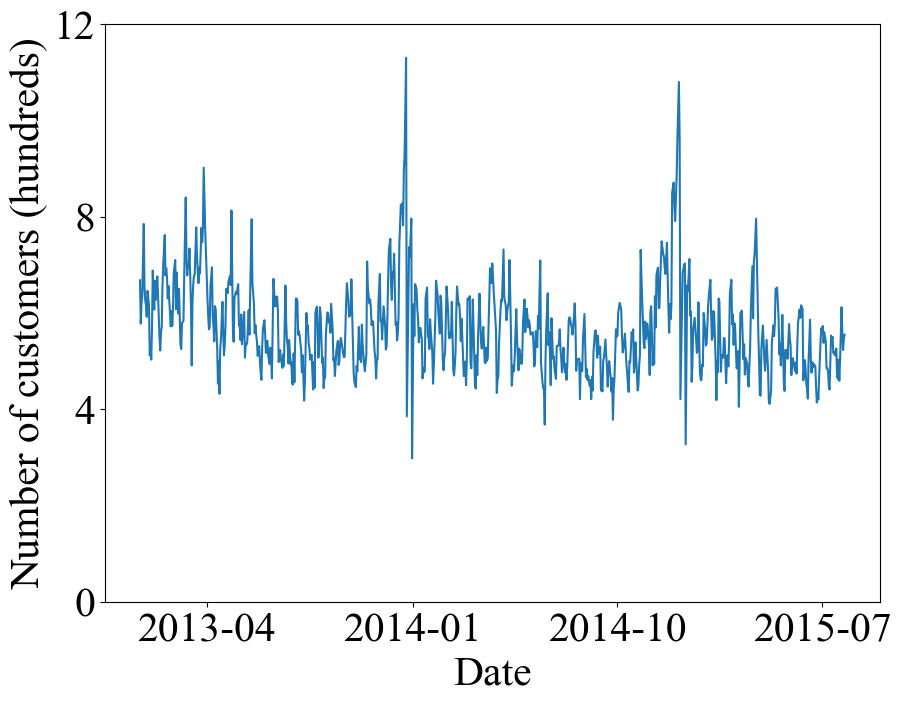
(a) Rossmann

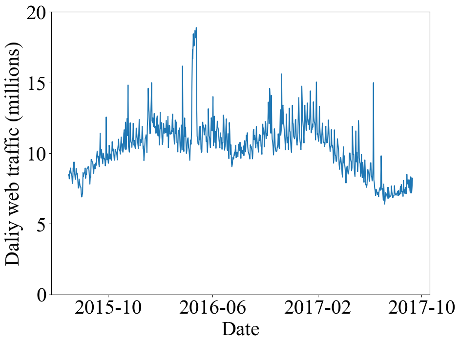
(b) Wikipedia

Figure 2. An example of a single time series from each dataset. (a) Daily number of customers that visited a single store in the Rossmann drug store chain from January 2013 to July 2015. The full dataset contains 1,115 stores. (b) Daily web traffic across Wikipedia French language pages from July 2015 to September 2017. The full dataset contains 9 languages.

We used two real-world datasets to represent the “demand” sequences in our experiments. Both datasets include multiple daily time series and are publicly available:

• Rossmann: This dataset contains the daily number of customers that visited each of 1,115 stores in the Rossmann drug store chain during a 781-day period in 2013-2015.

• Wikipedia: This dataset contains daily web traffic across Wikipedia.com pages of 9 different languages for an 803-day period from 2015 to 2017.

Fig. 2 contains example time series from each of these datasets.

Each instance of our experiment represented a single Nonstationary Newsvendor with Predictions problem, with the realized demands taken from a single time series in our data (either a single Rossmann store or a single lanaguage on Wikipedia). The overage and underage costs were constant within each instance, and without loss the two costs for an instance can be characterized by the corresponding critical quantile (specifically the ratio of the underage cost to the sum). The time horizon for each instance was a set number of days taken from the end of the time series, with the preceding days used to train one of four prediction methods. These predictions were also updated over the course of the instance at a set frequency. For the Wikipedia dataset, this yields a total of 2,880 possible instances, all of which were tested. The Rossmann dataset has multiple orders of magnitude more instances, so we simply randomly sampled 1,000 from this set. Table 2 describes all of the instances used.

	Rossmann	Wikipedia
Number of time series	1,115	9
Critical quantiles (%)	30,40,50,60,70	95,98,99,99.9
Experimental period (days)	300,400,500,600	300,400,500,600,700
Prediction update frequency (days)	2,4,10,20	2,4,10,20
Total number of instances	1,000 (sampled)	2,880 (exhaustive)

Table 2. Description of experimental instances.

For each instance, we applied the Shrinking-Time-Window Policy, Prediction Policy, and PERP. To generate predictions, we used four popular forecasting methods ranging from classical algorithms to the state-of-the art:

• Exponential Smoothing (Holt Winters): A classic algorithm based on a (linear) trend and seasonality decomposition as in eq. 2.2, known for its simplicity and robust performance. It is frequently used as a benchmark in forecasting competitions [3]. Tuning parameters: seasonality of length 50.

• ARIMA: Another classic algorithm that is rich enough to model a wide class of nonstationary time-series. Tuning parameters: $(p,q,r)=(3,2,5)$.

• Prophet: A recent algorithm developed by Facebook [1] based on a (piecewise-linear) trend and seasonality decomposition as in eq. 2.2, known to work well in practice with minimal tuning. Tuning parameters: software default.

• LightGBM: A recent algorithm developed by Microsoft [5] based on tree algorithms. Incidentally, LightGBM formed the core of most of the top entries in the recent $100,000 M5 Forecasting Challenge [4]. Tuning parameters: software default.

We treated the outputs of these methods as predictions of the mean demand. To estimate the demand distribution around this mean, we used the empirical distribution of the residuals of the same predictions on the training period. In practice, even if the prediction quality is good, the predictions of the first few days might incur large costs due to the noise/instability of the predictions. This may cause PERP to misidentify the prediction quality. Therefore we restrict PERP to following the predictions for the first 20 days, and only allow PERP to switch afterward – this is to prevent premature switching caused by the noise/instability of the predictions.

5.2. Results

Each instance yields three total costs: one incurred by PERP, and two incurred by the benchmark algorithms (the Shrinking-Time-Window and Prediction policies). The primary performance metric we report is a form of optimality gap. For an instance $I$, let $\mathrm{cost}^{\mathrm{prediction}}(I)$ be the cost of the Prediction Policy, and similarly define $\mathrm{cost}^{\mathrm{shrinking}}(I)$, $\mathrm{cost}^{\mathrm{PERP}}(I)$. Then the optimality gap (GAP) of PERP is defined as

$$\mathrm{GAP}(I)=\frac{\mathrm{cost}^{\mathrm{PERP}}(I)-\min\{\mathrm{cost}^{\mathrm{prediction}}(I),\mathrm{cost}^{\mathrm{shrinking}}(I)\}}{\max\{\mathrm{cost}^{\mathrm{prediction}}(I),\mathrm{cost}^{\mathrm{shrinking}}(I)\}-\min\{\mathrm{cost}^{\mathrm{prediction}}(I),\mathrm{cost}^{\mathrm{shrinking}}(I)\}}.$$

If we think of PERP as trying to achieve the minimum of the costs incurred by the two benchmark policies, then GAP measures the excess cost that PERP incurs on top of this minimum, normalized so that $\mathrm{GAP}=0$ implies that the minimum has been achieved, and $\mathrm{GAP}=1$ implies that the maximum of the two costs was incurred.

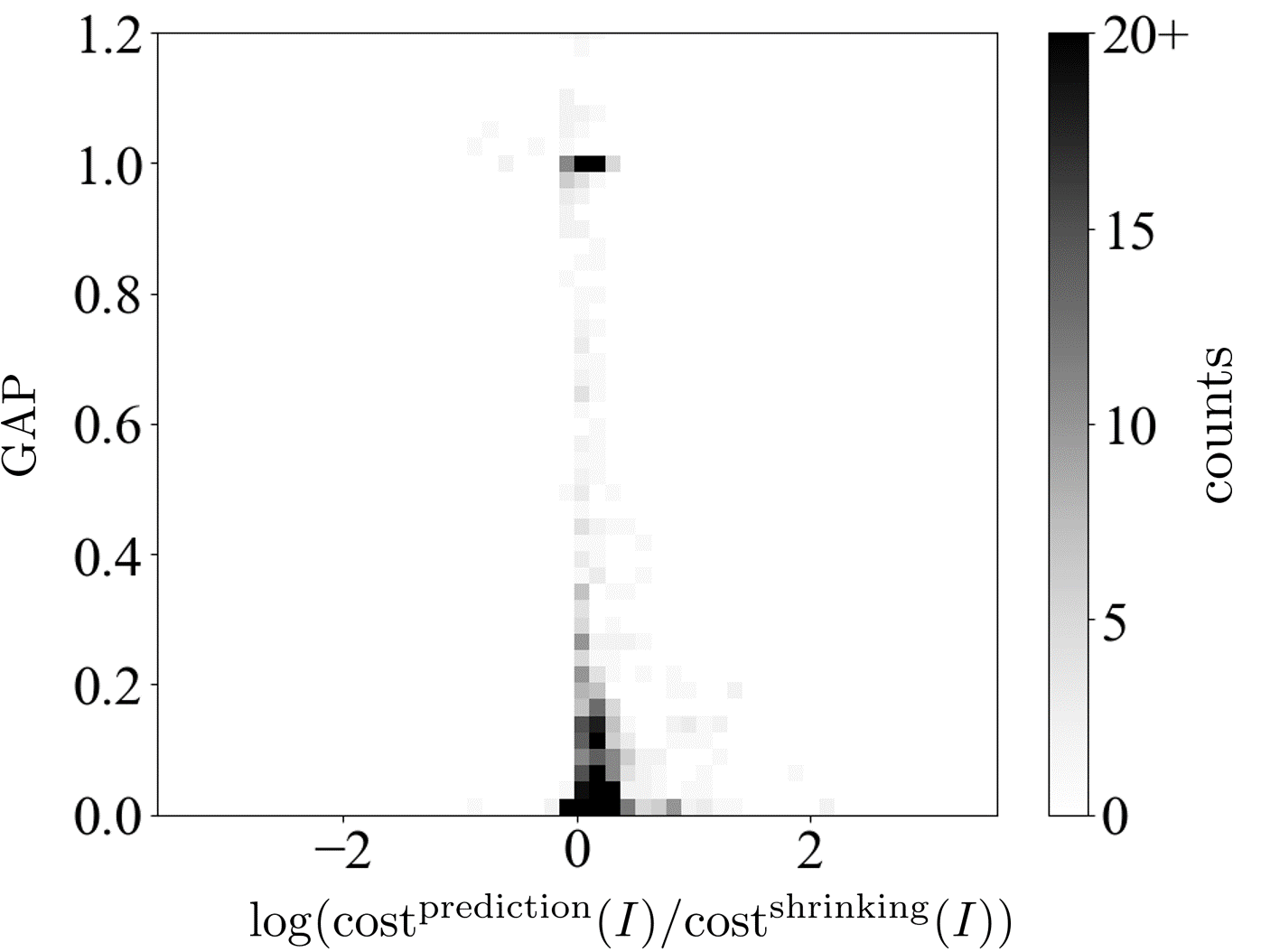
(a) GAPs of Rossmann

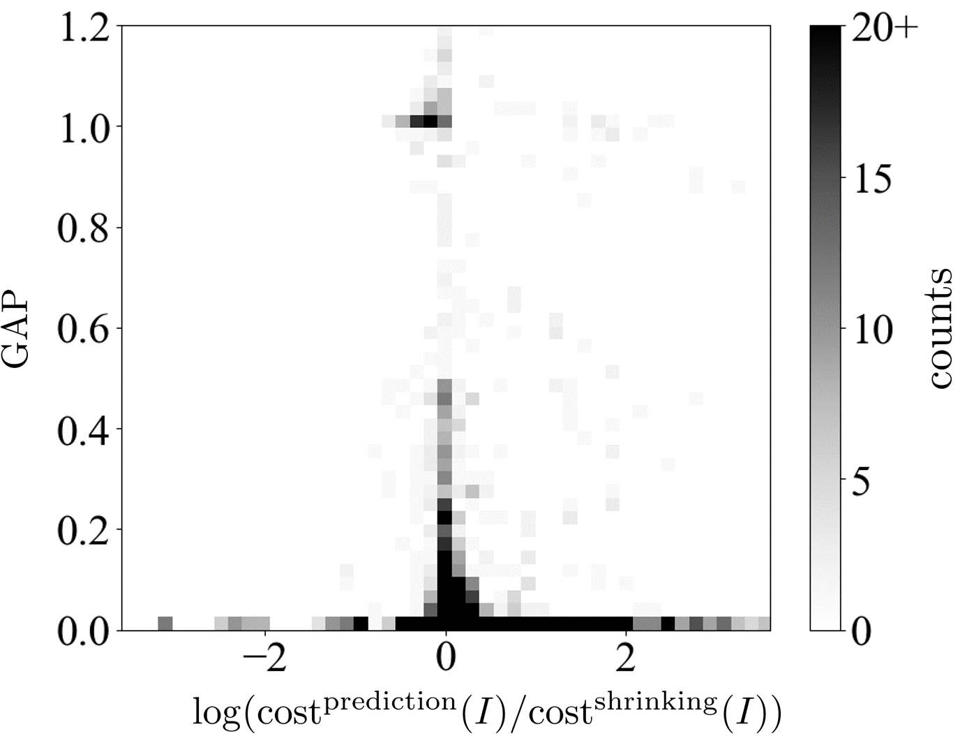
(b) GAPs of Wikipedia

Figure 3. (a) Histogram of GAPs across 1000 randoml-sampled instances on the Rossmann dataset.(b) Histogram of GAPs across 2880 instances on the Wikipedia dataset.

Experiments on the two datasets yield the histograms in Fig. 3. For each instance $I$, the value on the horizonal axis is $\log(\mathrm{cost}^{\mathrm{prediction}}(I)/\mathrm{cost}^{\mathrm{shrinking}}(I))$, which is greater than 0 if the Shrinking-Time-Window Policy has a lower cost, and less than 0 if the Prediction Policy has a lower cost. In the Rossman sample of 1000 instances, the Shrinking-Time-Window Policy has a lower cost 82.7% of the time and the Prediction Policy has a lower cost 17.3% of the time. In the Wikipedia sample of 2880 instances, the Shrinking-Time-Window Policy has a lower cost 81.9% of the time and the Prediction Policy has a lower cost 18.1% of the time. The values on the vertical axis are the GAPs. Note that most GAPs are small when the absolute values of the log difference are large. This shows PERP performs very well when the difference of costs between the Shrinking-Time-Window Policy and the Prediction Policy is large. On the other hand, there are instances where PERP has large GAPs, in particular there are instances with GAPs equal to 1 when the log difference of costs is close to 0. This happens because when the log difference of costs is close to 0, the cost of the Prediction Policy and the cost of the Shrinking-Time-Window Policy are close, so PERP may misidentify the prediction quality. Still, since the max cost and the min cost of the other two policies are close, even the GAPs are large in these instances, PERP doesn’t perform badly.

	Rossmann	Wikipedia
Average GAP with good predictions	0.26	0.40
Average GAP with bad predictions	0.28	0.07

Table 3. Description of experimental results.

We further divide the instances according to which of the Shrinking-Time-Window Policy and the Prediction Policy has lower cost in Fig. 4.

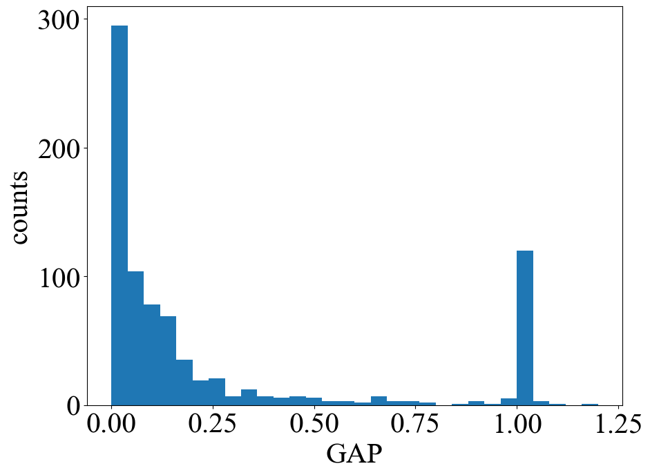
(a) Rossmann: Low Prediction Accuracy

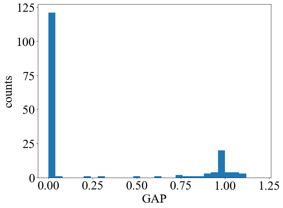
(b) Rossmann: High Prediction Accuracy

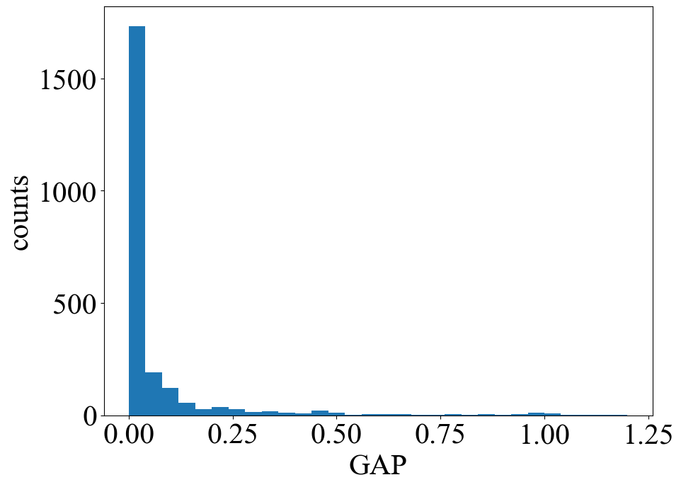
(c) Wikipedia: Low Prediction Accuracy

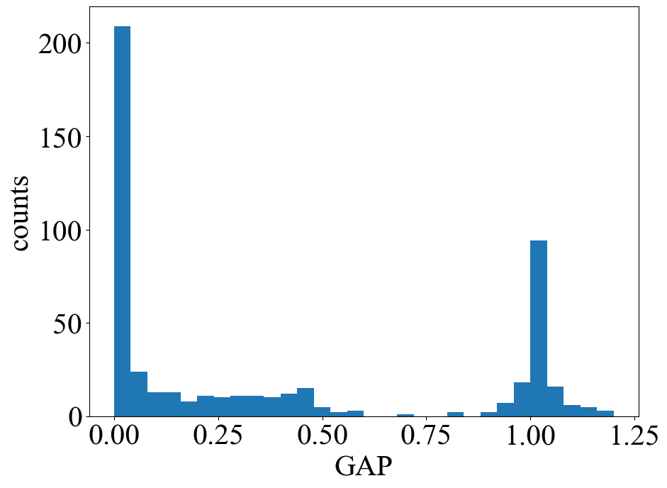
(d) Wikipedia: High Prediction Accuracy

Figure 4. Histograms of the GAPs for (a) 827 Rossmann instances for which the Shrinking-Time-Window Policy has lower cost, (b) 173 Rossmann instances for which the Prediction Policy has lower cost, 2358 Wikipedia instances for which the Shrinking-Time-Window Policy has lower cost, and (d) 522 Wikipedia instances for which the Prediction Policy has lower cost.

In the Rossman dataset, the average GAP is 0.258 on the 827 instances where the Shrinking-Time-Window Policy has a lower cost and 0.280 on the 173 instances where the Prediction Policy has a lower cost. In the Wikipedia dataset, the average GAP is 0.071 on the 2358 instances where the Shrinking-Time-Window Policy has a lower cost and 0.404 on the 522 instances where the Prediction Policy has a lower cost. In comparison, if we don’t know the prediction quality beforehand, uniformly random choosing between the Shrinking-Time-Window Policy and the Prediction Policy has an expected GAP of 0.5. Therefore PERP outperforms this natural benchmark in both cases of both datasets.

6. Conclusion

In this paper, we proposed a new model incorporating predictions into the nonstationary newsvendor problem. We first gave a complete analysis of the Nonstationary Newsvendor (without predictions) by proving a lower regret bound and developing the Shrinking-Time-Window Policy which achieves the lower bound up to log factors. Moreover, our model was the first nonstationary newsvendor model where the distribution and order quantities are allowed to be discrete. We then considered the Nonstationary Newsvendor with Predictions and proposed the Prediction-Error-Robust Policy, which does not need to know the prediction quality beforehand, and achieves nearly optimal minimax worst-cast regret.

Appendix A Preliminary Observations

For any time periods $a,b$, let $\mathcal{R}^{\pi}(T)[a,b]=\sup_{\bm{D}\in\mathcal{D}(v)}\mathbb{E}^{\pi}_{\bm{D}}\left\{\sum_{t=a}^{b}\left(C_{t}(\mu_{t},q_{t})-C_{t}(\mu_{t},q^{*}_{t})\right)\right\}$ be the regret incurred by the policy $\pi$ from time $a$ to time $b$. We make the following two useful observations:

Observation A.1.

For any policy $\pi$, $\mathcal{R}^{\pi}(T)[a,b]\leq C(b-a+1)$ for some universal constant $C\in(0,\infty)$.

Proof.

Because $\mu_{t}$ and $q_{t}$ are both bounded, $C_{t}(\mu_{t},q_{t})$ is also bounded in $[C_{\min},C_{\max}]$ where $C_{\min}=\inf_{\mu_{t}\in[\mu_{\min},\mu_{\max}],q_{t}\in Q}C_{t}(\mu_{t},q_{t})$ and $C_{\max}=\sup_{\mu_{t}\in[\mu_{\min},\mu_{\max}],q_{t}\in Q}C_{t}(\mu_{t},q_{t})$. Thus,

$$\mathcal{R}^{\pi}(T)[a,b]=\sup_{\bm{D}\in\mathcal{D}(v)}\mathbb{E}^{\pi}_{\bm{D}}\left\{\sum_{t=a}^{b}\left(C_{t}(\mu_{t},q_{t})-C_{t}(\mu_{t},q^{*}_{t})\right)\right\}\leq(C_{\max}-C_{\min})(b-a+1).$$

Take $C=(C_{\max}-C_{\min})$ gives the desired result. ∎

Observation A.2.

For any policy $\pi$ such that, from time $a$ to time $b$, $\pi$ first estimates the mean at time $t$ to be $\hat{\mu}_{t}\in[\mu_{\mathrm{min}},\mu_{\mathrm{max}}]$ for every $a\leq t\leq b$ and then order $q_{t}\in\text{argmin}_{q\in Q}C_{t}(\hat{\mu}_{t},q)$, we have $\mathcal{R}^{\pi}(T)[a,b]\leq C\cdot\sup_{\bm{D}\in\mathcal{D}(v)}\mathbb{E}^{\pi}_{\bm{D}}\left\{\sum_{t=a}^{b}|\hat{\mu}_{t}-\mu_{t}|\right\}$ for some universal constant $C\in(0,\infty)$.

Proof.

Let $\ell$ be the Lipschitz constant of $C(\cdot,q)$, then by Lemma 2.1

$$C_{t}(\mu_{t},q_{t})-C_{t}(\mu_{t},q_{t}^{*})\leq 2\ell|\hat{\mu}_{t}-\mu_{t}|.$$

Therefore,

$$\mathcal{R}^{\pi}(T)[a,b] = \sup_{\bm{D}\in\mathcal{D}(v)}\mathbb{E}^{\pi}_{\bm{D}}\left\{\sum_{t=a}^{b}\left(C_{t}(\mu_{t},q_{t})-C_{t}(\mu_{t},q^{*}_{t})\right)\right\}$$

$$\leq 2\ell\cdot\sup_{\bm{D}\in\mathcal{D}(v)}\mathbb{E}^{\pi}_{\bm{D}}\left\{\sum_{t=a}^{b}|\hat{\mu}_{t}-\mu_{t}|\right\}.$$

Taking $C=2\ell$ gives the desired result. ∎

Observation A.2 implies that any policy $\pi$ that estimates the mean accurately at each time achieves low regret.

Appendix B Proof of Lemma 3.1

Proof of Lemma 3.1..

Because our bounds are all asymptotic, we ignore the rounding and write $n=\kappa T^{(1-v)/2}$ to simplify the notation.

By Observation A.1, $\mathcal{R}^{\pi^{\mathrm{fixed}}}(T)[1,n]\leq C_{1}n<C_{1}T^{(3+v)/4}$ for some universal constant $C_{1}\in(0,\infty)$.

From now on we consider the time period from $t=n+1$ to $t=T$. We first upper bound the total estimation error of the mean $\sum_{t=n+1}^{T}|\hat{\mu}_{t}-\mu_{t}|$. Note that

$$\sum_{t=n+1}^{T}|\hat{\mu}_{t}-\mu_{t}| \overset{(a)}{\leq} \sum_{t=n+1}^{T}\left|\frac{1}{n}\sum_{s=t-n}^{t-1}d_{s}-\mu_{t}\right|$$

$$= \sum_{t=1}^{T}\left|\frac{1}{n}\sum_{s=t-n}^{t-1}(\mu_{s}+\epsilon_{s})-\mu_{t}\right|$$

$$= \sum_{t=n+1}^{T}\left|\frac{1}{n}\sum_{s=t-n}^{t-1}(\mu_{s}-\mu_{t})+\frac{1}{n}\sum_{s=t-n}^{t-1}\epsilon_{s}\right|$$

$$\leq \sum_{t=n+1}^{T}\left|\frac{1}{n}\sum_{s=t-n}^{t-1}(\mu_{s}-\mu_{t})\right|+\sum_{t=n+1}^{T}\left|\frac{1}{n}\sum_{s=t-n}^{t-1}\epsilon_{s}\right|,$$

where $(a)$ follows because $\hat{\mu}_{t}$ is the projection of $\frac{1}{n}\sum_{s=t-n}^{t-1}d_{s}$ on $[\mu_{\min},\mu_{\max}]$.

We bound these two parts separately through the following two lemmas.

Lemma B.1.

There exists a universal constant $C_{2}\in(0,\infty)$ such that

$$\sum_{t=n+1}^{T}\left|\frac{1}{n}\sum_{s=t-n}^{t-1}(\mu_{s}-\mu_{t})\right|\leq C_{2}T^{(3+v)/4}.$$

Proof of Lemma B.1..

For any $n+1\leq t\leq T$ we have

$$\left|\frac{1}{n}\sum_{s=t-n}^{t-1}\left(\mu_{s}-\mu_{t}\right)\right|\leq\frac{1}{n}\sum_{s=t-n}^{t-1}\left|\mu_{s}-\mu_{t}\right|\leq\max_{t-n\leq s\leq t-1}\left|\mu_{s}-\mu_{t}\right|.$$

Also, by bounded demand variation,

$$\sum_{t=n+1}^{T}\max_{t-n\leq s\leq t-1}\left|\mu_{s}-\mu_{t}\right|^{2} \overset{(a)}{=} \sum_{j=1}^{\lceil T/n\rceil}\sum_{i=1}^{n}\max_{(j-1)n+i\leq s\leq jn+i-1}\left|\mu_{s}-\mu_{t}\right|^{2}$$

$$\overset{(b)}{=} \sum_{i=1}^{n}\sum_{j=1}^{\lceil T/n\rceil}\max_{(j-1)n+i\leq s\leq jn+i-1}\left|\mu_{s}-\mu_{t}\right|^{2}$$

$$\overset{(c)}{\leq} nV_{\bm{\mu}}$$

$$\leq \kappa T^{(1+v)/2},$$

where $(a)$ is obtained by partitioning the sum into time windows, $(b)$ is obtained by exchanging the summations, and $(c)$ follows by the definition of demand variation $V_{\bm{\mu}}$ since $\{t_{j}=jn+i-1:j=0,1,\dots,\lceil T/n\rceil\}$ is a partition of $\{1,\dots,T\}$ for all $i=1,\dots,n$.

By Cauchy–Schwarz inequality,

$$\sum_{t=n+1}^{T}\max_{t-n\leq s\leq t-1}\left|\mu_{s}-\mu_{t}\right| \leq \sqrt{(T-n)\cdot\sum_{t=n+1}^{T}\max_{t-n\leq s\leq t-1}\left|\mu_{s}-\mu_{t}\right|^{2}}$$

$$\leq \sqrt{(T-n)\cdot\kappa T^{(1+v)/2}}$$

$$\leq \sqrt{\kappa}T^{(3+v)/4}.$$

Take $C_{2}=\sqrt{\kappa}$ gives the desired result. ∎

Lemma B.2.

There exists a universal constant $C_{3}\in(0,\infty)$ such that

$$\mathbb{E}^{\pi^{\mathrm{fixed}}}_{\bm{D}}\left\{\sum_{t=n+1}^{T}\left|\frac{1}{n}\sum_{s=t-n}^{t-1}\epsilon_{s}\right|\right\}\leq C_{3}T^{(3+v)/4}.$$

Proof of Lemma B.2..

Because each $D_{s}$ is sub-Gaussian, each $\epsilon_{s}$ is sub-Gaussian. Therefore there exists a constant $\delta_{s}<\infty$ where $\delta_{s}=\inf\{\delta^{\prime}\geq 0:\mathbb{E}[e^{\epsilon_{s}^{2}/\delta^{\prime 2}}]\leq 2\}$. Let $\delta=\max_{s=1,\dots,T}\delta_{s}$, then by Hoeffding’s inequality, for any $n+1\leq t\leq T$ we have

$$\mathbb{P}\left\{\left|\frac{1}{n}\sum_{s=t-n}^{t-1}\epsilon_{s}\right|\geq x\right\}\leq 2\text{ exp}\left(-\frac{\rho(nx)^{2}}{\sum_{s=t-n}^{t-1}\delta_{s}^{2}}\right)\leq 2\text{ exp}\left(-\frac{\rho n}{\delta^{2}}x^{2}\right),$$

where $\rho>0$ is a universal constant. Therefore we have

$$\mathbb{E}^{\pi^{\mathrm{fixed}}}_{\bm{D}}\left\{\left|\frac{1}{n}\sum_{s=t-n}^{t-1}\epsilon_{s}\right|\right\} = \int_{0}^{\infty}\mathbb{P}\left\{\left|\frac{1}{n}\sum_{s=t-n}^{t-1}\epsilon_{s}\right|\geq x\right\}dx$$

$$\leq \int_{0}^{\infty}2\text{ exp}\left(-\frac{\rho n}{\delta^{2}}x^{2}\right)dx$$

$$= \sqrt{\frac{\pi\delta^{2}}{\rho n}}$$

$$= \sqrt{\frac{\pi\delta^{2}}{\rho\kappa}}T^{(v-1)/4}.$$

Hence $\mathbb{E}^{\pi^{\mathrm{fixed}}}_{\bm{D}}\left\{\sum_{t=n+1}^{T}\left|\frac{1}{n}\sum_{s=t-n}^{t-1}\epsilon_{s}\right|\right\}\leq(T-n)\sqrt{\frac{\pi\delta^{2}}{\rho\kappa}}T^{(v-1)/4}\leq\sqrt{\frac{\pi\delta^{2}}{\rho\kappa}}T^{(3+v)/4}$. Take $C_{3}=\sqrt{\frac{\pi\delta^{2}}{\rho\kappa}}$ gives the desired result. ∎

Now we finish the proof of Lemma 3.1. With Lemma B.1 and Lemma B.2, we conclude that

$$\mathbb{E}^{\pi^{\mathrm{fixed}}}_{\bm{D}}\left\{\sum_{t=n+1}^{T}|\hat{\mu}_{t}-\mu_{t}|\right\} \leq \mathbb{E}^{\pi^{\mathrm{fixed}}}_{\bm{D}}\left\{\sum_{t=n+1}^{T}\left|\frac{1}{n}\sum_{s=t-n}^{t-1}(\mu_{s}-\mu_{t})\right|\right\}+\mathbb{E}^{\pi^{\mathrm{fixed}}}_{\bm{D}}\left\{\sum_{t=n+1}^{T}\left|\frac{1}{n}\sum_{s=t-n}^{t-1}\epsilon_{s}\right|\right\}$$

$$\leq (C_{2}+C_{3})T^{(3+v)/4}.$$

Therefore by Observation A.2 there exists a universal constant $C_{4}\in(0,\infty)$ such that

$$\mathcal{R}^{\pi^{\mathrm{fixed}}}(T) =\mathcal{R}^{\pi^{\mathrm{fixed}}}(T)[1,n]+\mathcal{R}^{\pi^{\mathrm{fixed}}}(T)[n+1,T]$$

$$\leq C_{1}T^{(3+v)/4}+C_{4}(C_{2}+C_{3})T^{(3+v)/4}$$

$$\leq(C_{1}+C_{4}(C_{2}+C_{3}))T^{(3+v)/4}.$$

Take $C=(C_{1}+C_{4}(C_{2}+C_{3}))$ we get $\mathcal{R}^{\pi^{\mathrm{fixed}}}(T)\leq CT^{(3+v)/4}$. ∎

Appendix C Proof of Theorem 3.1

Proof of Theorem 3.1..

Because our bounds are all asymptotic, we ignore the roundings and write $n_{i}=\kappa T^{(1-v_{i})/2}$ to simplify the notation.

By Observation A.1 $\mathcal{R}^{\pi^{\mathrm{shrinking}}}(T)[1,T^{3/4}]\leq C_{1}T^{3/4}$ for some universal constant $C_{1}\in(0,\infty)$.

From now on we consider the time periods after $T^{3/4}$. Let $\ell$ be the smallest index such that $v_{\ell}\geq v$, then $v_{\ell}\leq(1+\frac{1}{\log T})v$, so

(C.1) $$T^{v_{\ell}}\leq T^{(1+1/\log T)v}=e^{v}T^{v}\leq eT^{v}.$$

First, we show that $\hat{\mu}_{t}^{j}$ is close to $\mu_{t}$ when $j\geq\ell$ via the following lemma:

Lemma C.1.

For every $j\geq\ell$ with the corresponding window size $n_{j}=\kappa T^{(1-v_{j})/2}$, there exists a universal constant $\gamma>0$ such that

$$\mathbb{P}\left\{\sum_{t=n_{j}+1}^{T}\left|\hat{\mu}_{t}^{j}-\mu_{t}\right|\geq\left(\gamma\sqrt{\log T}+\sqrt{\kappa}\right)\cdot T^{(3+v_{j})/4}\right\}\leq\frac{2}{T^{3/2}}.$$

Proof of Lemma C.1..

Same as in the proof of Lemma B.2, by Hoeffding’s inequality for any $n_{j}+1\leq t\leq T$ we have

$$\mathbb{P}\left\{\left|\frac{1}{n_{j}}\sum_{s=t-n_{j}}^{t-1}\epsilon_{s}\right|\geq x\right\}\leq 2\text{ exp}\left(-\frac{\rho(n_{j}x)^{2}}{\sum_{s=t-n_{j}}^{t-1}\delta_{s}^{2}}\right)\leq 2\text{ exp}\left(-\frac{\rho n_{j}}{\delta^{2}}x^{2}\right),$$

where $\rho$ and $\delta$ are the same as in the previous proof. Set $\gamma>0$ to be large enough so that

(C.2) $$\frac{\rho\kappa\gamma^{2}}{\delta^{2}}\geq\frac{5}{2}.$$

Take $x=\gamma\sqrt{\log T}\cdot T^{(v_{j}-1)/4}$ and plug in $n_{j}=\kappa T^{(1-v_{j})/2}$ yields

$$\mathbb{P}\left\{\left|\frac{1}{n_{j}}\sum_{s=t-n_{j}}^{t-1}\epsilon_{s}\right|\geq\gamma\sqrt{\log T}\cdot T^{(v_{j}-1)/4}\right\}\leq 2\text{ exp}\left(-\frac{\rho\kappa\gamma^{2}}{\delta^{2}}\log T\right)\leq\frac{2}{T^{5/2}}.$$

Then we get

$$\mathbb{P}\left\{\sum_{t=n_{j}+1}^{T}\left|\frac{1}{n_{j}}\sum_{s=t-n_{j}}^{t-1}\epsilon_{s}\right|\geq\gamma\sqrt{\log T}\cdot T^{(3+v_{j})/4}\right\} \leq\mathbb{P}\left\{\max_{n_{j}+1\leq t\leq T}\left|\frac{1}{n_{j}}\sum_{s=t-n_{j}}^{t-1}\epsilon_{s}\right|\geq\gamma\sqrt{\log T}\cdot T^{(v_{j}-1)/4}\right\}$$

$$\overset{(a)}{\leq}T\cdot\mathbb{P}\left\{\left|\frac{1}{n_{j}}\sum_{s=t-n_{j}}^{t-1}\epsilon_{s}\right|\geq\gamma\sqrt{\log T}\cdot T^{(v_{j}-1)/4}\right\}$$

$$\leq\frac{2}{T^{3/2}},$$

where $(a)$ follows by union bound. Note that since $V_{\mathbb{\bm{\mu}}}\leq T^{v}\leq T^{v_{j}}$, by Lemma B.1 we know $\sum_{t=n_{j}+1}^{T}\left|\frac{1}{n_{j}}\sum_{s=t-n_{j}}^{t-1}(\mu_{s}-\mu_{t})\right|\leq\sqrt{\kappa}T^{(3+v_{j})/4}$, and in the proof of Lemma 3.1 we have

$$\sum_{t=n_{j}+1}^{T}|\hat{\mu}_{t}^{j}-\mu_{t}|\leq\sum_{t=n_{j}+1}^{T}\left|\frac{1}{n_{j}}\sum_{s=t-n_{j}}^{t-1}(\mu_{s}-\mu_{t})\right|+\sum_{t=n_{j}+1}^{T}\left|\frac{1}{n_{j}}\sum_{s=t-n_{j}}^{t-1}\epsilon_{s}\right|.$$

Therefore

$$\quad\mathbb{P}\left\{\sum_{t=n_{j}+1}^{T}\left|\hat{\mu}_{t}^{j}-\mu_{t}\right|\geq\left(\gamma\sqrt{\log T}+\sqrt{\kappa}\right)\cdot T^{(3+v_{j})/4}\right\}$$

$$\leq\mathbb{P}\left\{\sum_{t=n_{j}+1}^{T}\left|\frac{1}{n_{j}}\sum_{s=t-n_{j}}^{t-1}(\mu_{s}-\mu_{t})\right|+\sum_{t=n_{j}+1}^{T}\left|\frac{1}{n_{j}}\sum_{s=t-n_{j}}^{t-1}\epsilon_{s}\right|\geq\left(\gamma\sqrt{\log T}+\sqrt{\kappa}\right)\cdot T^{(3+v_{j})/4}\right\}$$

$$\leq\mathbb{P}\left\{\sum_{t=n_{j}+1}^{T}\left|\frac{1}{n_{j}}\sum_{s=t-n_{j}}^{t-1}\epsilon_{s}\right|\geq\gamma\sqrt{\log T}\cdot T^{(3+v_{j})/4}\right\}$$

$$\leq\frac{2}{T^{3/2}}.$$

∎

For each $j\geq\ell$, let $E_{j}$ be the event $\left\{\sum_{t=n_{j}+1}^{T}\left|\hat{\mu}_{t}^{j}-\mu_{t}\right|\geq\left(\gamma\sqrt{\log T}+\sqrt{\kappa}\right)\cdot T^{(3+v_{j})/4}\right\}$, then $\mathbb{P}(E_{j})\leq\frac{2}{T^{3/2}}$ for each $j$. First we assume that $E_{j}$ does not happen for any $j\geq\ell$. We break the proof into three lemmas.

Lemma C.2.

Each time an if condition happens, for the current $i$ we have $i<\ell$. Therefore $i\leq\ell$ throughout the algorithm.

Proof of Lemma C.2.

Suppose an if condition happens at time $t$ triggered by some index $j>i$, then $\sum_{s=t_{\textbf{if}}}^{t}|\hat{\mu}_{s}^{i}-\hat{\mu}_{s}^{j}|\geq 2\left(\gamma\sqrt{\log T}+\sqrt{\kappa}\right)T^{(3+v_{j})/4}$. Suppose for the sake of contradiction that $i\geq\ell$, then

$$\sum_{s=t_{\textbf{if}}}^{t}|\hat{\mu}_{s}^{i}-\hat{\mu}_{s}^{j}| \overset{(a)}{\leq}\sum_{s=t_{\textbf{if}}}^{t}|\hat{\mu}_{s}^{i}-\mu_{s}|+\sum_{s=t_{\textbf{if}}}^{t}|\hat{\mu}_{s}^{j}-\mu_{s}|$$

$$\overset{(b)}{\leq}\sum_{s=n_{i}+1}^{T}|\hat{\mu}_{s}^{i}-\mu_{s}|+\sum_{s=n_{j}+1}^{T}|\hat{\mu}_{s}^{j}-\mu_{s}|$$

$$\overset{(c)}{<}\left(\gamma\sqrt{\log T}+\sqrt{\kappa}\right)\cdot T^{(3+v_{i})/4}+\left(\gamma\sqrt{\log T}+\sqrt{\kappa}\right)\cdot T^{(3+v_{j})/4}$$

$$\overset{(d)}{<}2\left(\gamma\sqrt{\log T}+\sqrt{\kappa}\right)\cdot T^{(3+v_{j})/4},$$

where $(a)$ comes from the triangle inequality and $(b)$ is because $t_{\textbf{if}}>T^{3/4}$ and $n_{i},n_{j}\leq\kappa T^{1/2}$; since $j>i\geq\ell$, by our assumption neither $E_{i}$ nor $E_{j}$ occurs, so we get $(c)$; $(d)$ follows since $v_{j}>v_{i}$. This contradicts with $\sum_{s=t_{\textbf{if}}}^{t}|\hat{\mu}_{s}^{i}-\hat{\mu}_{s}^{j}|\geq 2\left(\gamma\sqrt{\log T}+\sqrt{\kappa}\right)T^{(3+v_{j})/4}$. Therefore, we must have $i<\ell$. Because the index $i$ never decreases and can only increase by 1 each time an if condition happens, $i\leq\ell$ throughout the algorithm.

Lemma C.3.

Suppose two consecutive if conditions occur at time $t^{\prime}$ and $t^{\prime\prime}$, then $\mathcal{R}^{\pi^{\mathrm{shrinking}}}(T)[t^{\prime},t^{\prime\prime}-1]\leq C_{2}T^{(3+v)/4}\sqrt{\log T}$ for some universal constant $C_{2}\in(0,\infty)$.

∎

Proof of Lemma C.3.

At time $t$ where $t^{\prime}\leq t\leq t^{\prime\prime}-1$, by Lemma C.2 $i<\ell$. We have

$$\sum_{s=t^{\prime}+1}^{t^{\prime\prime}-1}|\hat{\mu}_{s}^{i}-\mu_{s}| \overset{(a)}{\leq}\sum_{s=t^{\prime}+1}^{t^{\prime\prime}-1}|\hat{\mu}_{s}^{\ell}-\mu_{s}|+\sum_{s=t^{\prime}+1}^{t^{\prime\prime}-1}|\hat{\mu}_{s}^{i}-\hat{\mu}_{s}^{\ell}|$$

$$\overset{(b)}{\leq}\sum_{s=n_{i}+1}^{T}|\hat{\mu}_{s}^{\ell}-\mu_{s}|+\sum_{s=t^{\prime}+1}^{t^{\prime\prime}-1}|\hat{\mu}_{s}^{i}-\hat{\mu}_{s}^{\ell}|$$

$$\overset{(c)}{<}\left(\gamma\sqrt{\log T}+\sqrt{\kappa}\right)\cdot T^{(3+v_{\ell})/4}+2\left(\gamma\sqrt{\log T}+\sqrt{\kappa}\right)\cdot T^{(3+v_{\ell})/4}$$

$$\overset{(d)}{\leq}3e^{1/4}\left(\gamma\sqrt{\log T}+\sqrt{\kappa}\right)\cdot T^{(3+v)/4},$$

where $(a)$ comes from the triangle inequality and $(b)$ is because $t^{\prime}>T^{3/4}$ and $n_{i}\leq\kappa T^{1/2}$; the first part of $(c)$ follows by our assumption that $E_{\ell}$ does not occur, and the second part of $(c)$ follows since the if condition is not triggered between time $t^{\prime}$ and time $t^{\prime\prime}-1$; $(d)$ follows by eq. C.1. Then by Observation A.2 there exists a universal constant $C^{\prime}\in(0,\infty)$ such that

$$\mathcal{R}^{\pi^{\mathrm{shrinking}}}(T)[t^{\prime},t^{\prime\prime}-1]\leq C^{\prime}\sum_{s=t^{\prime}}^{t^{\prime\prime}-1}|\hat{\mu}_{s}^{i}-\mu_{s}|\leq 3e^{1/4}C^{\prime}\left(\gamma\sqrt{\log T}+\sqrt{\kappa}\right)\cdot T^{(3+v)/4}.$$

Take $C_{2}=3e^{1/4}C^{\prime}\left(\gamma+\sqrt{\kappa}\right)$ gives the desired result. ∎

The above proof also works for $\mathcal{R}^{\pi^{\mathrm{shrinking}}}(T)[T^{3/4}+1,t_{\mathrm{first}}-1]$ if the first if condition happens at time $t_{\mathrm{first}}$, or $\mathcal{R}^{\pi^{\mathrm{shrinking}}}(T)[T^{3/4}+1,T]$ if the if condition never happens. Note that the index $i$ never decreases and increases by 1 if and only if the if condition happens. Suppose that the last if condition happens at time $t_{\mathrm{last}}$, then we have

$$\mathcal{R}^{\pi^{\mathrm{shrinking}}}(T)[T^{3/4}+1,t_{\mathrm{last}}-1] \overset{(a)}{\leq}(\text{\# of {if} conditions happened})\cdot C_{2}T^{(3+v)/4}\sqrt{\log T}$$

$$\overset{(b)}{\leq}kC_{2}T^{(3+v)/4}\sqrt{\log T}$$

$$\overset{(c)}{\approx}C_{2}\log_{1+\frac{1}{\log T}}(\log T)\cdot T^{(3+v)/4}\sqrt{\log T}$$

$$=C_{2}\frac{\log(T)}{\log(1+\frac{1}{\log T})}T^{(3+v)/4}\sqrt{\log T}$$

$$\overset{(d)}{\approx}C_{2}T^{(3+v)/4}\log^{5/2}T$$

for some universal constant $C_{2}\in(0,\infty)$. Here $(a)$ follows by Lemma C.3, $(b)$ is because the maximum index of $v_{i}$ is $k$, $(c)$ is because $v_{k-1}<1\leq v_{k}$, and $(d)$ follows by $\log(1+x)\approx x$ when $x$ is small.

Finally, we analyze the time periods after $t_{\mathrm{last}}$.

Lemma C.4.

$\mathcal{R}^{\pi^{\mathrm{shrinking}}}(T)[t_{\mathrm{last}},T]\leq C_{3}T^{(3+v)/4}\sqrt{\log T}$ for some universal constant $C_{3}\in(0,\infty)$.

Proof of Lemma C.4.

Because the if condition happens at $t_{\mathrm{last}}$, by Lemma C.2 either $i<\ell$ or $i=\ell$. Suppose $i<\ell$, then similar to Lemma C.3 we have

$$\sum_{s=t_{\mathrm{last}}}^{T}|\hat{\mu}_{s}^{i}-\mu_{s}| \overset{(a)}{\leq}\sum_{s=t_{\mathrm{last}}}^{T}|\hat{\mu}_{s}^{\ell}-\mu_{s}|+\sum_{s=t_{\mathrm{last}}}^{T}|\hat{\mu}_{s}^{i}-\hat{\mu}_{s}^{\ell}|$$

$$\overset{(b)}{\leq}\sum_{s=n_{i}+1}^{T}|\hat{\mu}_{s}^{\ell}-\mu_{s}|+\sum_{s=t_{\mathrm{last}}}^{T}|\hat{\mu}_{s}^{i}-\hat{\mu}_{s}^{\ell}|$$

$$\overset{(c)}{<}\left(\gamma\sqrt{\log T}+\sqrt{\kappa}\right)\cdot T^{(3+v_{\ell})/4}+2\left(\gamma\sqrt{\log T}+\sqrt{\kappa}\right)\cdot T^{(3+v_{\ell})/4}$$

$$\overset{(d)}{\leq}3e^{1/4}\left(\gamma\sqrt{\log T}+\sqrt{\kappa}\right)\cdot T^{(3+v)/4},$$

where $(a)$ comes from the triangle inequality and $(b)$ is because $t_{\mathrm{last}}>T^{3/4}$ and $n_{i}\leq\kappa T^{1/2}$; the first part of $(c)$ follows by our assumption that $E_{\ell}$ does not occur, and the second part of $(c)$ follows since the if condition is never triggered after $t_{\mathrm{last}}$; $(d)$ follows by eq. C.1. By Observation A.2, we get $\mathcal{R}^{\pi^{\mathrm{shrinking}}}(T)[t_{\mathrm{last}},T]\leq 3e^{1/4}C^{\prime}\left(\gamma\sqrt{\log T}+\sqrt{\kappa}\right)\cdot T^{(3+v)/4}$ for some universal constant $C^{\prime}\in(0,\infty)$.

On the other hand, suppose $i=\ell$. Note $V_{\bm{\mu}}\leq T^{v}\leq T^{v_{\ell}}$ and after time $t_{\mathrm{last}}$ the Shrinking-Time-Window Policy just performs the Fixed-Time-Window Policy with variation parameter $v_{\ell}$, so by Lemma 3.1 $\mathcal{R}^{\pi^{\mathrm{shrinking}}}(T)[t_{\mathrm{last}},T]\leq C^{\prime\prime}T^{(3+v_{\ell})/4}\leq C^{\prime\prime}e^{1/4}T^{(3+v)/4}$ for some universal constant $C^{\prime\prime}\in(0,\infty)$, where the last inequality again follows by eq. C.1.

Taking $C_{3}=3e^{1/4}\max\{C^{\prime}\left(\gamma+\sqrt{\kappa}\right),C^{\prime\prime}\}$ we get $\mathcal{R}^{\pi^{\mathrm{shrinking}}}(T)[t_{\mathrm{last}},T]\leq C_{3}T^{(3+v)/4}\sqrt{\log T}$ in both cases. ∎

Combining everything above, in the case where $E_{j}$ doesn’t happen for any $j\geq\ell$, we get

$$\mathcal{R}^{\pi^{\mathrm{shrinking}}}(T) =\mathcal{R}^{\pi^{\mathrm{shrinking}}}(T)[1,T^{3/4}]+\mathcal{R}^{\pi^{\mathrm{shrinking}}}(T)[T^{3/4}+1,t_{\mathrm{last}}-1]$$

$$\quad\text{ }+\mathcal{R}^{\pi^{\mathrm{shrinking}}}(T)[t_{\mathrm{last}},T]$$

$$\leq C_{1}T^{3/4}+C_{2}T^{(3+v)/4}\log^{5/2}T+C_{3}T^{(3+v)/4}\sqrt{\log T}.$$

Now let us consider the case where $E_{j}$ happens for some $j\geq\ell$. Because $\mathbb{P}\{E_{j}\}\leq\frac{2}{T^{3/2}}$ for each $j\geq\ell$, by union bound

$$\mathbb{P}\left\{E_{j}\text{ happens for some }j\geq\ell\right\}\leq\frac{2}{T^{3/2}}\cdot|\mathcal{V}|\leq\frac{2}{T},$$

where the last inequality follows by $|\mathcal{V}|=k\approx\log^{2}T$. By Observation A.1 we always have $\mathcal{R}^{\pi^{\mathrm{shrinking}}}(T)\leq c_{4}T$ for some universal constant $C_{4}\in(0,\infty)$. Therefore in summary we have

$$\mathcal{R}^{\pi^{\mathrm{shrinking}}}(T) \leq\mathbb{P}\{E_{j}\text{ doesn't happen for any }j\geq\ell\}\left(C_{1}T^{3/4}+C_{2}T^{(3+v)/4}\log^{5/2}T+C_{3}T^{(3+v)/4}\sqrt{\log T}\right)$$

$$\quad+\mathbb{P}\left\{E_{j}\text{ happens for some }j\geq\ell\right\}C_{4}T$$

$$\leq C_{1}T^{3/4}+C_{2}T^{(3+v)/4}\log^{5/2}T+C_{3}T^{(3+v)/4}\sqrt{\log T}+2C_{4}.$$

Therefore, there exists some universal constant $C\in(0,\infty)$ such that $\mathcal{R}^{\pi^{\mathrm{shrinking}}}(T)\leq CT^{(3+v)/4}\log^{5/2}T$.

∎

Appendix D Proof of Proposition 3.1, Proposition 4.1, and 4.1b)

Note that Proposition 3.1 and Observation 4.1b) can be easily deduced from Proposition 4.1 by setting $a=1$ and $v=1$ respectively, so it suffices to prove Proposition 4.1.

Proof of Proposition 4.1..

We construct the following worst-case problem instance: divide the time horizon $T$ into cycles of length $T^{(1-v)/2}$ (since the analysis below is compatible with scaling, for simplicity we assume $T^{(1-v)/2}$ is an integer), so there are $T^{(1+v)/2}$ cycles. Assume that the demand distribution within each cycle is a Bernoulli distribution that equals to $1$ with probability $p$ and equals to $0$ with probability $1-p$. At the beginning of each cycle, we set the $p$ of the upcoming cycle to be either $\frac{1}{2}+\frac{1}{\sqrt{20}}T^{(v-1)/4}$ or $\frac{1}{2}-\frac{1}{\sqrt{20}}T^{(v-1)/4}$, each with probability $\frac{1}{2}$. Set $Q=\mathbb{R}_{+}$ and $b_{t}=h_{t}=1$ for all $t$, so the optimal ordering amount is the median of the demand distribution at each time.

First we show that the demand variation $V_{\bm{\mu}}$ is at most $T^{v}$. Note that since $\mu_{t}=p$ is fixed within each cycle, only the times between cycles contribute to the demand variation. Suppose the cycle changes between time $t$ and $t+1$, then $\left(\mu_{t+1}-\mu_{t}\right)^{2}\leq(\frac{2}{\sqrt{20}}T^{(v-1)/4})^{2}=\frac{1}{5}T^{(v-1)/2}$. Because there are $T^{(1+v)/2}$ cycles, $V_{\bm{\mu}}\leq T^{(1+v)/2}\cdot\frac{1}{5}T^{(v-1)/2}=\frac{1}{5}T^{v}$.

Then we add predictions into the instance. We divide the analysis into two cases.

Case 1: $a\geq\frac{3+v}{4}$.

For each $t$ we set $a_{t}$ to be either $\frac{1}{2}+\frac{1}{\sqrt{20}}T^{(v-1)/4}$ or $\frac{1}{2}-\frac{1}{\sqrt{20}}T^{(v-1)/4}$, each with probability $\frac{1}{2}$. Then because each $a_{t}$ and $\mu_{t}$ are i.i.d., $a_{t}$ provides no information about $\mu_{t}$. Hence the predictions are useless in this instance. Note that

$$\sum_{t=1}^{T}|a_{t}-\mu_{t}|\leq T\cdot\frac{2}{\sqrt{20}}T^{(v-1)/4}=\frac{1}{\sqrt{5}}T^{(3+v)/4}\leq\frac{1}{\sqrt{5}}T^{a},$$

so the prediction accuracy is within $T^{a}$.

Then we analyze the amount of regret incurred. For $i=1,\dots,T^{(1-v)/2}$, let $P_{i}$, $Q_{i}$ be i.i.d. distributions respectively, where $P_{i}\sim\text{Bernoulli }(\frac{1}{2}+\frac{1}{\sqrt{20}}T^{(v-1)/4})$ and $Q_{i}\sim\text{Bernoulli }(\frac{1}{2}-\frac{1}{\sqrt{20}}T^{(v-1)/4})$. Then the Kullback-Leibler divergence of $P_{i}$ from $Q_{i}$ is

$$D_{\text{KL}}\left(P_{i}\parallel Q_{i}\right)= \left(\frac{1}{2}+\frac{1}{\sqrt{20}}T^{(v-1)/4}\right)\log\left(\frac{\frac{1}{2}+\frac{1}{\sqrt{20}}T^{(v-1)/4}}{\frac{1}{2}-\frac{1}{\sqrt{20}}T^{(v-1)/4}}\right)$$

$$+\left(\frac{1}{2}-\frac{1}{\sqrt{20}}T^{(v-1)/4}\right)\log\left(\frac{\frac{1}{2}-\frac{1}{\sqrt{20}}T^{(v-1)/4}}{\frac{1}{2}+\frac{1}{\sqrt{20}}T^{(v-1)/4}}\right).$$

We show that $D_{\text{KL}}\left(P_{i}\parallel Q_{i}\right)\leq\frac{13}{20}T^{(v-1)/2}$. Let $x=\frac{1}{\sqrt{20}}T^{(v-1)/4}$, then because $v\in[0,1]$, $x\in[0,\frac{1}{\sqrt{20}}]$. Note that the $D_{\text{KL}}\left(P_{i}\parallel Q_{i}\right)=13x^{2}$ for $x=0$, and we have

$$\frac{d}{dx}D_{\text{KL}}\left(P_{i}\parallel Q_{i}\right)\biggm{|}_{x=0}=0=\frac{d}{dx}13x^{2}\biggm{|}_{x=0}$$

and

$$\frac{d^{2}}{dx^{2}}D_{\text{KL}}\left(P_{i}\parallel Q_{i}\right)=\frac{1}{(x^{2}-0.25)^{2}}<26=\frac{d^{2}}{dx^{2}}13x^{2}$$

for $x\in[0,\frac{1}{\sqrt{20}}]$. This shows $13x^{2}-D_{\text{KL}}\left(P_{i}\parallel Q_{i}\right)=0$ at $x=0$, the first derivative is $0$ at $x=0$, and the second derivative is non-negative for $x\in[0,\frac{1}{\sqrt{20}}]$. This implies $D_{\text{KL}}\left(P_{i}\parallel Q_{i}\right)\leq 13x^{2}=\frac{13}{20}T^{(v-1)/2}$.

Let $P=\sum_{i=1}^{T^{(1-v)/2}}P_{i}$ and $Q=\sum_{i=1}^{T^{(1-v)/2}}Q_{i}$ be the two possible demand distributions within a cycle, then because $P_{i}$’s are i.i.d. and $Q_{i}$’s are i.i.d.,

$$D_{\text{KL}}\left(P\parallel Q\right)=\sum_{i=1}^{T^{(1-v)/2}}D_{\text{KL}}\left(P_{i}\parallel Q_{i}\right)\leq T^{(1-v)/2}\cdot\frac{13}{20}T^{(v-1)/2}=\frac{13}{20}.$$

We claim that within each cycle, any attempt to distinguish between $P$ and $Q$ has at least a constant probability of making a mistake, i.e., one cannot effectively estimate the $p$ value within each cycle. Let $\mathcal{C}:\{0,1\}^{T^{(1-v)/2}}\to\{P,Q\}$ be any classifier that takes the demand observations within a cycle as inputs and determine the true demand distribution of this cycle. Let $E=\mathcal{C}^{-1}(P)$ be the event where $\mathcal{C}$ classifies the demand observations as from demand distribution $P$, then by Pinsker’s inequality,

$$|P(E)-Q(E)|\leq\sqrt{\frac{1}{2}D_{\text{KL}}\left(P\parallel Q\right)}\leq\sqrt{\frac{13}{40}},$$

where $P(E)$ is the probability of $E$ happening under the condition that the true demand distribution is $P$, and the same for $Q(E)$. Therefore we have

$$\mathbb{P}\left\{\mathcal{C}\text{ makes a mistake}\right\} = P(E^{c})+Q(E)$$

$$\geq P(E^{c})+P(E)-\sqrt{\frac{13}{40}}$$

$$= 1-\sqrt{\frac{13}{40}}.$$

Hence for any classifier $\mathcal{C}$ the probability of making the wrong guess of $p$ in the current cycle is at least $1-\sqrt{\frac{13}{40}}$.

Note for demand distribution $P_{i}$, $q^{*}=1$ and $C(\mu_{P_{i}},0)-C(\mu_{P_{i}},1)=\frac{1}{2}+\frac{1}{\sqrt{20}}T^{(v-1)/4}-(1-(\frac{1}{2}+\frac{1}{\sqrt{20}}T^{(v-1)/4}))=\frac{1}{\sqrt{5}}T^{(v-1)/4}$, and similarly for demand distribution $Q_{i}$, $q^{*}=0$ and $C(\mu_{Q_{i}},1)-C(\mu_{Q_{i}},0)=(1-(\frac{1}{2}-\frac{1}{\sqrt{20}}T^{(v-1)/4}))-(\frac{1}{2}-\frac{1}{\sqrt{20}}T^{(v-1)/4})=\frac{1}{\sqrt{5}}T^{(v-1)/4}$. Therefore each wrong guess of $p$ incurs a difference between $C(\mu_{t},q_{t})$ and $C(\mu_{t},q^{*}_{t})$ by $\frac{1}{\sqrt{5}}T^{(v-1)/4}$, which incurs a regret of $C(\mu_{t},q_{t})-C(\mu_{t},q^{*}_{t})=\frac{1}{\sqrt{5}}T^{(v-1)/4}.$ Therefore over $T$ time periods the expected total regret of any General Policy $\pi$ satisfies

$$\mathcal{R}^{\pi}(T) \geq \left(1-\sqrt{\frac{13}{40}}\right)\frac{1}{\sqrt{5}}T^{(v-1)/4}\cdot T$$

$$= \left(1-\sqrt{\frac{13}{40}}\right)\frac{1}{\sqrt{5}}T^{(3+v)/4}$$

$$= \left(1-\sqrt{\frac{13}{40}}\right)\frac{1}{\sqrt{5}}T^{\min\{(3+v)/4,a\}},$$

where the last equality follows from the assumption that $a\geq\frac{3+v}{4}$. Take $c=\left(1-\sqrt{\frac{13}{40}}\right)\frac{1}{\sqrt{5}}$ gives the desired result.

Case 2: $a<\frac{3+v}{4}$.

Note that $a<\frac{3+v}{4}$ implies $a-\frac{1+3v}{4}<\frac{1-v}{2}$ and $T^{(1-v)/2}$ is the length of each cycle. For the first $T^{a-\frac{1+3v}{4}}$ time periods of each cycle, we set $a_{t}$ to be either $\frac{1}{2}+\frac{1}{\sqrt{20}}T^{(v-1)/4}$ or $\frac{1}{2}-\frac{1}{\sqrt{20}}T^{(v-1)/4}$, each with probability $\frac{1}{2}$. For the other time periods we set $a_{t}=\mu_{t}$. Then, similar as in the case above, the predictions are useless for the first $T^{a-\frac{1+3v}{4}}$ time periods of each cycle in this instance. Since there are $T^{(1+v)/2}$ number of cycles,

$$\sum_{t=1}^{T}|a_{t}-\mu_{t}|\leq T^{(1+v)/2}\cdot T^{a-\frac{1+3v}{4}}\cdot\frac{2}{\sqrt{20}}T^{(v-1)/4}=\frac{1}{\sqrt{5}}T^{a},$$

so the prediction accuracy is within $T^{a}$.

Again, the same analysis as the case above shows that for the first $T^{a-\frac{1+3v}{4}}$ time periods of each cycle, the probability of making the wrong guess of $p$ in the current cycle is at least $1-\sqrt{\frac{13}{40}}$. Also, each wrong guess of $p$ incurs a regret of $\frac{2}{\sqrt{5}}T^{(v-1)/4}$. Because there are $T^{(1+v)/2}$ number of cycles, over $T$ time periods the expected total regret of any General Policy $\pi$ satisfies

$$\mathcal{R}^{\pi}(T) \geq\left(1-\sqrt{\frac{13}{40}}\right)\frac{1}{\sqrt{5}}T^{(v-1)/4}\cdot T^{(1+v)/2}\cdot T^{a-\frac{1+3v}{4}}$$

$$=\left(1-\sqrt{\frac{13}{40}}\right)\frac{1}{\sqrt{5}}T^{a}$$

$$=\left(1-\sqrt{\frac{13}{40}}\right)\frac{1}{\sqrt{5}}T^{\min\{(3+v)/4,a\}},$$

where the last equality follows from the assumption that $a<\frac{3+v}{4}$. Take $c=\left(1-\sqrt{\frac{13}{40}}\right)\frac{1}{\sqrt{5}}$ gives the desired result. ∎

Appendix E Proof of Proposition 4.2

Proof of Proposition 4.2..

Set $Q=\mathbb{R}_{+}$ and $b_{t}=h_{t}=1$ for all $t$, so the optimal ordering amount is the median of the demand distribution at each time. We construct the following two problem instances:

Instance 1: for all $t$, set $D^{(1)}_{t}\sim Unif(0,2)$. Then $\mu^{(1)}_{t}=1$. Set $a^{(1)}_{t}=d^{(1)}_{t}$, where $d^{(1)}_{t}$ is the realization of $D^{(1)}_{t}$. Since $\mu^{(1)}_{t}=1$ for all $t$, the variation parameter $v^{(1)}=0$. Because $a^{(1)}_{t}$ is a constant away from $\mu_{t}^{(1)}$ with probability 1, $a^{(1)}=1$. Because the optimal order amount is $q_{t}^{(1)*}=\mu_{t}^{(1)}$, $C(\mu_{t}^{(1)},q_{t}^{(1)*})=\mathbb{E}\left[b_{t}(D^{(1)}_{t}-\mu_{t}^{(1)})^{+}+h_{t}(\mu_{t}^{(1)}-D^{(1)}_{t})^{+}\right]=\mathbb{E}\left[|D^{(1)}_{t}-1|\right]=\frac{1}{2}$.

Instance 2: for all $t$, set $D^{(2)}_{t}=\mu_{t}^{(2)}\sim Unif(0,2)$. i.e., $D_{t}^{(2)}$ is a one-point distribution. Set $a_{t}^{(2)}=d_{t}^{(2)}$, where $d_{t}^{(2)}$ is the realization of $D_{t}^{(2)}$. Since $\mu_{t}^{(2)}$ changes by a constant amount from $\mu_{t-1}^{(2)}$ with probability 1 throughout $t=2,\dots,T$, the variation parameter $v^{(2)}=1$. Because $a_{t}^{(2)}=\mu_{t}^{(2)}$ for every $t$, $a^{(2)}=0$. Because the optimal order amount is $q_{t}^{(2)*}=\mu_{t}^{(2)}$, $C(\mu_{t}^{(2)},q_{t}^{(2)*})=\mathbb{E}\left[b_{t}(D^{(2)}_{t}-\mu_{t}^{(2)})^{+}+h_{t}(\mu_{t}^{(2)}-D^{(2)}_{t})^{+}\right]=0$.

Note that a General Policy can only observe information on $a_{t}$’s and $d_{t}$’s. Because $a_{t}^{(1)}=d_{t}^{(1)}$ and $a_{t}^{(2)}=d_{t}^{(2)}$ have the same distribution for every $t$, no General Policies can distinguish between the two instances. For any General Policy $\pi$, let $q_{t}$ be its output at time $t$. Without loss of generality, we may assume $q_{t}\in[0,2]$ since any other ordering amount is clearly sub-optimal. Then

$$C(\mu_{t}^{(1)},q_{t})=\mathbb{E}\left[b_{t}(D^{(1)}_{t}-q_{t})^{+}+h_{t}(q_{t}-D^{(1)}_{t})^{+}\right]=\frac{q_{t}^{2}+(2-q_{t})^{2}}{4}\geq\frac{1}{2}$$

and

$$C(\mu_{t}^{(2)},q_{t})=\mathbb{E}\left[b_{t}(D^{(2)}_{t}-q_{t})^{+}+h_{t}(q_{t}-D^{(2)}_{t})^{+}\right]=\frac{2-q_{t}}{2}+\frac{q_{t}}{2}=1.$$

Let $\mathcal{R}^{\pi}[I_{1}](T)$ denote the regret of $\pi$ on instance 1 and $\mathcal{R}^{\pi}[I_{2}](T)$ denote the regret of $\pi$ on instance 2, then

$$\mathcal{R}^{\pi}[I_{1}](T)+\mathcal{R}^{\pi}[I_{2}](T) = \sum_{t=1}^{T}\left(C(\mu_{t}^{(1)},q_{t})-C(\mu_{t}^{(1)},q_{t}^{(1)*})\right)+\sum_{t=1}^{T}\left(C(\mu_{t}^{(2)},q_{t})-C(\mu_{t}^{(2)},q_{t}^{(2)*})\right)$$

$$\geq \sum_{t=1}^{T}\left(\frac{1}{2}-\frac{1}{2}\right)+\sum_{t=1}^{T}\left(1-0\right)$$

$$= T.$$

Because $\mathcal{R}^{\pi}[I_{1}](T)+\mathcal{R}^{\pi}[I_{2}](T)\geq T$, any General Policy $\pi$ incurs regret at least $0.5T$ on at least one of the instances. Since no General Policy can distinguish between the two instances, we can always choose the worse one of the two instances to feed to the policy. Also, since $v^{(1)}=0$, $a^{(1)}=1$, $v^{(2)}=1$, $a^{(2)}=0$, in both instances we have $a\neq\frac{3+v}{4}$. Therefore for any General Policy $\pi$ there always exists a problem instance with $a\neq\frac{3+v}{4}$ such that $\mathcal{R}^{\pi}(T)\geq 0.5T=\Omega(T^{\max\{(3+v)/4,a\}})$ on the instance. ∎

Appendix F Proof of Theorem 4.1

Proof of Theorem 4.1..

Because our bounds are all asymptotic, we ignore the rounding and write $n=\kappa T^{(1-v)/2}$ to simplify the notation.

Because $\pi^{\mathrm{PERP}}_{t}=\pi^{a}_{t}$ for $t$ from $1$ to $n$, by Observation 4.1 $\mathcal{R}^{\pi^{\mathrm{PERP}}}(T)[1,n]=\mathcal{R}^{\pi^{a}}(T)[1,n]\leq C_{1}^{\prime}T^{a}$ for some universal constant $C_{1}^{\prime}\in(0,\infty)$. Also, by Observation A.1, since $n=\kappa T^{(1-v)/2}<\kappa T^{(3+v)/4}$, there exists some universal constant $C_{1}^{\prime\prime}\in(0,\infty)$ such that $\mathcal{R}^{\pi^{\mathrm{PERP}}}(T)[1,n]\leq C_{1}^{\prime\prime}T^{(3+v)/4}$. Take $C_{1}=\max\{C_{1}^{\prime},C_{1}^{\prime\prime}\}$ we get $\mathcal{R}^{\pi^{\mathrm{PERP}}}(T)[1,n]\leq C_{1}T^{\min\{(3+v)/4,a\}}\sqrt{\log T}.$

Now we consider the time periods after time $n+1$. First, same as in the proof of Lemma B.2, by Hoeffding’s inequality for any $n+1\leq t\leq T$ we have

$$\mathbb{P}\left\{\left|\frac{1}{n}\sum_{s=t-n}^{t-1}\epsilon_{s}\right|\geq x\right\}\leq 2\exp\left(-\frac{\rho(nx)^{2}}{\sum_{s=t-n}^{t-1}\delta_{s}^{2}}\right)\leq 2\exp\left(-\frac{\rho n}{\delta^{2}}x^{2}\right),$$

where $\rho$ and $\delta$ are the same as in the previous proof. Set $\gamma>0$ to be large enough so that

(F.1) $$\frac{\rho\kappa\gamma^{2}}{\delta^{2}}\geq 2.$$

Take $x=\gamma\sqrt{\log T}\cdot T^{(v-1)/4}$ and plug in $n=\kappa T^{(1-v)/2}$ yields

$$\mathbb{P}\left\{\left|\frac{1}{n}\sum_{s=t-n}^{t-1}\epsilon_{s}\right|\geq\gamma\sqrt{\log T}\cdot T^{(v-1)/4}\right\}\leq 2\exp\left(-\frac{\rho\kappa\gamma^{2}}{\delta^{2}}\log T\right)\leq\frac{2}{T^{2}}.$$

Then we get

$$\mathbb{P}\left\{\sum_{t=n+1}^{T}\left|\frac{1}{n}\sum_{s=t-n}^{t-1}\epsilon_{s}\right|\geq\gamma\sqrt{\log T}\cdot T^{(3+v)/4}\right\} \leq \mathbb{P}\left\{\max_{n+1\leq t\leq T}\left|\frac{1}{n}\sum_{s=t-n}^{t-1}\epsilon_{s}\right|\geq\gamma\sqrt{\log T}\cdot T^{(v-1)/4}\right\}$$

$$\stackrel{{\scriptstyle(a)}}{{\leq}} T\cdot\mathbb{P}\left\{\left|\frac{1}{n}\sum_{s=t-n}^{t-1}\epsilon_{s}\right|\geq\gamma\sqrt{\log T}\cdot T^{(v-1)/4}\right\}$$

$$\leq \frac{2}{T},$$

where (a) follows by union bound. Note Lemma B.1 says $\sum_{t=n+1}^{T}\left|\frac{1}{n}\sum_{s=t-n}^{t-1}\left(\mu_{s}-\mu_{t}\right)\right|\leq\sqrt{\kappa}T^{(3+v)/4}$, and in the proof of Lemma 3.1 we have

$$\sum_{t=n+1}^{T}\left|\hat{\mu}_{t}^{\mathrm{fixed}}-\mu_{t}\right|\leq\sum_{t=n+1}^{T}\left|\frac{1}{n}\sum_{s=t-n}^{t-1}\left(\mu_{s}-\mu_{t}\right)\right|+\sum_{t=n+1}^{T}\left|\frac{1}{n}\sum_{s=t-n}^{t-1}\epsilon_{s}\right|.$$

Therefore

$$\quad\mathbb{P}\left\{\sum_{t=n+1}^{T}\left|\hat{\mu}_{t}^{\mathrm{fixed}}-\mu_{t}\right|\geq\left(\gamma\sqrt{\log T}+\sqrt{\kappa}\right)\cdot T^{(3+v)/4}\right\}$$

$$\leq\mathbb{P}\left\{\sum_{t=n+1}^{T}\left|\frac{1}{n}\sum_{s=t-n}^{t-1}(\mu_{s}-\mu_{t})\right|+\sum_{t=n+1}^{T}\left|\frac{1}{n}\sum_{s=t-n}^{t-1}\epsilon_{s}\right|\geq\left(\gamma\sqrt{\log T}+\sqrt{\kappa}\right)\cdot T^{(3+v)/4}\right\}$$

$$\leq\mathbb{P}\left\{\sum_{t=n+1}^{T}\left|\frac{1}{n}\sum_{s=t-n}^{t-1}\epsilon_{s}\right|\geq\gamma\sqrt{\log T}\cdot T^{(3+v)/4}\right\}$$

$$\leq\frac{2}{T}.$$

Because once the if condition in PERP is triggered we break the for loop, the if condition can happen at most once thoughout the algorithm. We consider two cases separately depending on whether the if condition happens or not:

Case 1: the if condition happens at some time $s$.

First, suppose $\sum_{t=n+1}^{T}\left|\hat{\mu}_{t}^{\mathrm{fixed}}-\mu_{t}\right|<(\gamma\sqrt{\log T}+\sqrt{\kappa})\cdot T^{(3+v)/4}$, then because the if condition happens at time $s$,

$$T^{a} = \sum_{t=1}^{T}\left|a_{t}-\mu_{t}\right|$$

$$\stackrel{{\scriptstyle(a)}}{{\geq}} \sum_{t=1}^{s}\left|\hat{\mu}_{t}^{a}-\mu_{t}\right|$$

$$\stackrel{{\scriptstyle(b)}}{{\geq}} \sum_{t=1}^{s}\left|\hat{\mu}_{t}^{a}-\hat{\mu}_{t}^{\mathrm{fixed}}\right|-\sum_{t=1}^{s}\left|\hat{\mu}_{t}^{\mathrm{fixed}}-\mu_{t}\right|$$

$$\stackrel{{\scriptstyle(c)}}{{\geq}} T^{(3+v)/4},$$

where $a_{t}=\hat{\mu}_{t}^{a}$ gives $(a),(b)$ follows by triangle inequality, and $(c)$ follows by the the if condition. This shows $a\geq\frac{3+v}{4}$, so $\min\left\{\frac{3+v}{4},a\right\}=\frac{3+v}{4}$. Note that between time $n+1$ and time $s-1$ we have:

$$\sum_{t=n+1}^{s-1}\left|\hat{\mu}_{t}^{a}-\mu_{t}\right| \stackrel{{\scriptstyle(a)}}{{\leq}} \sum_{t=n+1}^{s-1}\left|\hat{\mu}_{t}^{a}-\hat{\mu}_{t}^{\mathrm{fixed}}\right|+\sum_{t=n+1}^{s-1}\left|\hat{\mu}_{t}^{\mathrm{fixed}}-\mu_{t}\right|$$

$$\stackrel{{\scriptstyle(b)}}{{\leq}} (2\gamma\sqrt{\log T}+2\sqrt{\kappa}+1)\cdot T^{(3+v)/4},$$

where $(a)$ follows by triangle inequality and $(b)$ follows by the if condition (note by the algorithm’s construction $s\geq n+1$; for the simplicity of writing we assume $s-1\geq n+1$, and the case $s=n+1$ follows similarly). Then by Observation A.2, let $\ell$ be the Lipschitz constant, we have

$$\mathcal{R}^{\pi^{\mathrm{PERP}}}(T)[n+1,s-1] = \sup_{\bm{D}\in\mathcal{D}(v)}\mathbb{E}_{D,a}^{\pi^{\mathrm{PERP}}}\left\{\sum_{t=n+1}^{s-1}\left(C\left(\mu_{t},q_{t}\right)-C\left(\mu_{t},q_{t}^{*}\right)\right)\right\}$$

$$\stackrel{{\scriptstyle(a)}}{{\leq}} 2\ell\cdot\sup_{\bm{D}\in\mathcal{D}(v)}\mathbb{E}_{D,a}^{\pi^{\mathrm{PERP}}}\left\{\sum_{t=n+1}^{s-1}\left|\hat{\mu}_{t}^{a}-\mu_{t}\right|\right\}$$

$$\leq 2\ell(2\gamma\sqrt{\log T}+2\sqrt{\kappa}+1)\cdot T^{(3+v)/4},$$

where $(a)$ is because $\pi^{\mathrm{PERP}}=\pi^{a}$ before time $s$. Hence $\mathcal{R}^{\pi^{\mathrm{PERP}}}(T)[n+1,s-1]$ is on the order of $T^{(3+v)/4}\sqrt{\log T}$, so there exists some universal constant $C_{2}\in(0,\infty)$ such that $\mathcal{R}^{\pi^{\mathrm{PERP}}}(T)[n+1,s-1]\leq$ $C_{2}T^{(3+v)/4}\sqrt{\log T}$. Also, since after time $s$ we have $\pi^{\mathrm{PERP}}=\pi^{\mathrm{fixed}}$, by Lemma 3.1 there exists some universal constant $C_{3}\in(0,\infty)$ such that

$$\mathcal{R}^{\pi^{\mathrm{PERP}}}(T)[s,T]=\mathcal{R}^{\pi^{\mathrm{fixed}}}(T)[s,T]\leq\mathcal{R}^{\pi^{\mathrm{fixed}}}(T)\leq C_{3}T^{(3+v)/4}\sqrt{\log T}.$$

In summary, if $\sum_{t=n+1}^{T}\left|\hat{\mu}_{t}^{\mathrm{fixed}}-\mu_{t}\right|<(\gamma\sqrt{\log T}+\sqrt{\kappa})\cdot T^{(3+v)/4}$, we have

$$\mathcal{R}^{\pi^{\mathrm{PERP}}}(T) =\mathcal{R}^{\pi^{\mathrm{PERP}}}(T)[1,n]+\mathcal{R}^{\pi^{\mathrm{PERP}}}(T)[n+1,s-1]+\mathcal{R}^{\pi^{\mathrm{PERP}}}(T)[s,T]$$

$$\leq\left(C_{1}+C_{2}+C_{3}\right)T^{(3+v)/4}\sqrt{\log T}$$

$$=\left(C_{1}+C_{2}+C_{3}\right)T^{\min\{(3+v)/4,a\}}\sqrt{\log T},$$

where the last equality is because $\min\left\{\frac{3+v}{4},a\right\}=\frac{3+v}{4}$.

Second, suppose $\sum_{t=n+1}^{T}\left|\hat{\mu}_{t}^{\text{fixed}}-\mu_{t}\right|\geq(\gamma\sqrt{\log T}+\sqrt{\kappa})\cdot T^{(3+v)/4}$. By Observation A.1 there exists some universal constant $C_{4}\in(0,\infty)$ such that $\mathcal{R}^{\pi^{\mathrm{PERP}}}(T)\leq C_{4}T.$ Therefore combining the above two scenarios we get

$$\mathcal{R}^{\pi^{\mathrm{PERP}}}(T)\leq \mathbb{P}\left\{\sum_{t=n+1}^{T}\left|\hat{\mu}_{t}^{\mathrm{fixed}}-\mu_{t}\right|<(\gamma\sqrt{\log T}+\sqrt{\kappa})\cdot T^{(3+v)/4}\right\}\left(C_{1}+C_{2}+C_{3}\right)T^{\min\{(3+v)/4,a\}}\sqrt{\log T}$$

$$+\mathbb{P}\left\{\sum_{t=n+1}^{T}\left|\hat{\mu}_{t}^{\mathrm{fixed}}-\mu_{t}\right|\geq(\gamma\sqrt{\log T}+\sqrt{\kappa})\cdot T^{(3+v)/4}\right\}C_{4}T$$

$$\leq \left(C_{1}+C_{2}+C_{3}\right)T^{\min\{(3+v)/4,a\}}\sqrt{\log T}+\frac{2}{T}\cdot C_{4}T$$

$$= \left(C_{1}+C_{2}+C_{3}\right)T^{\min\{(3+v)/4,a\}}\sqrt{\log T}+2C_{4}.$$

Hence $\mathcal{R}^{\pi^{\mathrm{PERP}}}(T)\leq CT^{\min\{(3+v)/4,a\}}\sqrt{\log T}$ for some universal constant $C\in(0,\infty)$.

Case 2: the if condition does not happen.

In this case $\pi^{\mathrm{PERP}}=\pi^{a}$, so by Observation 4.1a) we immediately have $\mathcal{R}^{\pi^{\mathrm{PERP}}}(T)\leq C_{5}T^{a}\sqrt{\log T}$ for some universal constant $C_{5}\in(0,\infty)$. Also, following the same analysis as the part of Case 1 where an if condition has not happened, i.e., between time $n+1$ and time $s-1$, we get $\mathcal{R}^{\pi^{\mathrm{PERP}}}(T)[n+1,T]\leq$ $2l(2\gamma\sqrt{\log T}+2\sqrt{\kappa}+1)\cdot T^{(3+v)/4}\leq C_{6}T^{(3+v)/4}\sqrt{\log T}$ for some universal constant $C_{6}\in(0,\infty)$. Then we have $\mathcal{R}^{\pi^{\mathrm{PERP}}}(T)=\mathcal{R}^{\pi^{\mathrm{PERP}}}(T)[1,n]+\mathcal{R}^{\pi^{\mathrm{PERP}}}(T)[n+1,T]\leq\left(C_{1}+C_{6}\right)T^{(3+v)/4}\sqrt{\log T}$. Hence take $C=\max\left\{C_{5},C_{1}+C_{6}\right\}$ we have $\mathcal{R}^{\pi^{\mathrm{PERP}}}(T)\leq CT^{\min\{(3+v)/4,a\}}\sqrt{\log T}$.

∎

References

- [1] Sean J. Taylor and Benjamin Letham, “Forecasting at scale,” The American Statistician, 72(1), 37–45, 2018.
- [2] Francis Y. Edgeworth, “The mathematical theory of banking,” Journal of the Royal Statistical Society, 51(1), 113–127, 1888.
- [3] Spyros Makridakis and Michele Hibon, “The M3-Competition: results, conclusions, and implications,” International Journal of Forecasting, 16(4), 451–476, 2000.
- [4] Spyros Makridakis, Evangelos Spiliotis, and Vassilios Assimakopoulos, “M5 accuracy competition: Results, findings, and conclusions,” International Journal of Forecasting, 38(4), 1346–1364, 2022.
- [5] Guolin Ke, Qi Meng, Thomas Finley, Taifeng Wang, Wei Chen, Weidong Ma, Qiwei Ye, and Tie-Yan Liu, “Lightgbm: A highly efficient gradient boosting decision tree,” Advances in Neural Information Processing Systems, 30, 2017.
- [6] N. Bora Keskin, Xu Min, and Jing-Sheng Jeannette Song, “The nonstationary newsvendor: Data-driven nonparametric learning,” Available at SSRN 3866171, 2023.
- [7] Retsef Levi, Georgia Perakis, and Joline Uichanco, “The data-driven newsvendor problem: New bounds and insights,” Operations Research, 63(6), 1294–1306, 2015.
- [8] Paul Dütting, Silvio Lattanzi, Renato Paes Leme, and Sergei Vassilvitskii, “Secretaries with advice,” in Proceedings of the 22nd ACM Conference on Economics and Computation, pp. 409–429, 2021.
- [9] Kenneth Joseph Arrow, Samuel Karlin, Herbert E Scarf, and others, “Studies in the mathematical theory of inventory and production,” 1958, Stanford University Press.
- [10] Herbert Scarf, K. Arrow, S. Karlin, and P. Suppes, “The optimality of (S, s) policies in the dynamic inventory problem,” in Optimal pricing, inflation, and the cost of price adjustment, pp. 49–56, 1960, MIT Press Cambridge.
- [11] Herbert Scarf, “Bayes solutions of the statistical inventory problem,” The Annals of Mathematical Statistics, 30(2), 490–508, 1959, JSTOR.
- [12] William S Lovejoy, “Myopic policies for some inventory models with uncertain demand distributions,” Management Science, 36(6), 724–738, 1990, INFORMS.
- [13] Katy S Azoury, “Bayes solution to dynamic inventory models under unknown demand distribution,” Management Science, 31(9), 1150–1160, 1985, INFORMS.
- [14] Samuel Karlin, “Dynamic inventory policy with varying stochastic demands,” Management Science, 6(3), 231–258, 1960, INFORMS.
- [15] Donald L Iglehart, “The dynamic inventory problem with unknown demand distribution,” Management Science, 10(3), 429–440, 1964, INFORMS.
- [16] Liwan H Liyanage and J. George Shanthikumar, “A practical inventory control policy using operational statistics,” Operations Research Letters, 33(4), 341–348, 2005, Elsevier.
- [17] Woonghee Tim Huh and Paat Rusmevichientong, “A nonparametric asymptotic analysis of inventory planning with censored demand,” Mathematics of Operations Research, 34(1), 103–123, 2009, INFORMS.
- [18] Gah-Yi Ban and Cynthia Rudin, “The big data newsvendor: Practical insights from machine learning,” Operations Research, 67(1), 90–108, 2019, INFORMS.
- [19] Afshin Oroojlooyjadid, Lawrence V Snyder, and Martin Takáč, “Applying deep learning to the newsvendor problem,” IISE Transactions, 52(4), 444–463, 2020, Taylor & Francis.
- [20] Anton J. Kleywegt, Alexander Shapiro, and Tito Homem-de-Mello, “The sample average approximation method for stochastic discrete optimization,” SIAM Journal on Optimization, 12(2), 479–502, 2002, SIAM.
- [21] Alexander Shapiro, “Monte Carlo sampling methods,” Handbooks in Operations Research and Management Science, 10, 353–425, 2003, Elsevier.
- [22] Retsef Levi, Robin O. Roundy, and David B. Shmoys, “Provably near-optimal sampling-based policies for stochastic inventory control models,” Mathematics of Operations Research, 32(4), 821–839, 2007.
- [23] Apostolos N. Burnetas and Craig E. Smith, “Adaptive ordering and pricing for perishable products,” Operations Research, 48(3), 436–443, 2000, INFORMS.
- [24] Sumit Kunnumkal and Huseyin Topaloglu, “Using stochastic approximation methods to compute optimal base-stock levels in inventory control problems,” Operations Research, 56(3), 646–664, 2008, INFORMS.
- [25] Gregory A. Godfrey and Warren B. Powell, “An adaptive, distribution-free algorithm for the newsvendor problem with censored demands, with applications to inventory and distribution,” Management Science, 47(8), 1101–1112, 2001, INFORMS.
- [26] Warren Powell, Andrzej Ruszczyński, and Huseyin Topaloglu, “Learning algorithms for separable approximations of discrete stochastic optimization problems,” Mathematics of Operations Research, 29(4), 814–836, 2004, INFORMS.
- [27] N. Bora Keskin and Assaf Zeevi, “Chasing demand: Learning and earning in a changing environment,” Mathematics of Operations Research, 42(2), 277–307, 2017, INFORMS.
- [28] James T. Treharne and Charles R. Sox, “Adaptive inventory control for nonstationary demand and partial information,” Management Science, 48(5), 607–624, 2002, INFORMS.
- [29] Yossi Aviv and Amit Pazgal, “A partially observed Markov decision process for dynamic pricing,” Management Science, 51(9), 1400–1416, 2005, INFORMS.
- [30] Boxiao Chen, Xiuli Chao, and Hyun-Soo Ahn, “Coordinating pricing and inventory replenishment with nonparametric demand learning,” Operations Research, 67(4), 1035–1052, 2019, INFORMS.
- [31] Omar Besbes, Yonatan Gur, and Assaf Zeevi, “Stochastic multi-armed-bandit problem with non-stationary rewards,” Advances in Neural Information Processing Systems, 27, 2014.
- [32] Omar Besbes, Yonatan Gur, and Assaf Zeevi, “Non-stationary stochastic optimization,” Operations Research, 63(5), 1227–1244, 2015, INFORMS.
- [33] Santiago Balseiro, Christian Kroer, and Rachitesh Kumar, “Single-leg revenue management with advice,” arXiv preprint arXiv:2202.10939, 2022.
- [34] Andres Munoz and Sergei Vassilvitskii, “Revenue optimization with approximate bid predictions,” Advances in Neural Information Processing Systems, 30, 2017.
- [35] Thodoris Lykouris and Sergei Vassilvitskii, “Competitive caching with machine learned advice,” Journal of the ACM (JACM), 68(4), 1–25, 2021, ACM New York, NY.
- [36] Dhruv Rohatgi, “Near-optimal bounds for online caching with machine learned advice,” in Proceedings of the Fourteenth Annual ACM-SIAM Symposium on Discrete Algorithms, 1834–1845, 2020, SIAM.
- [37] Silvio Lattanzi, Thomas Lavastida, Benjamin Moseley, and Sergei Vassilvitskii, “Online scheduling via learned weights,” in Proceedings of the Fourteenth Annual ACM-SIAM Symposium on Discrete Algorithms, 1859–1877, 2020, SIAM.
- [38] Omar Besbes and Alp Muharremoglu, “On implications of demand censoring in the newsvendor problem,” Management Science, 59(6), 1407–1424, 2013, INFORMS.
- [39] Luhao Zhang, Jincheng Yang, and Rui Gao, “Optimal robust policy for feature-based newsvendor,” Management Science, Forthcoming, 2023.
- [40] Jakob Huber, Sebastian Müller, Moritz Fleischmann, and Heiner Stuckenschmidt, “A data-driven newsvendor problem: From data to decision,” European Journal of Operational Research, 278(3), 904–915, 2019, Elsevier.
- [41] Silvio Lattanzi, Thomas Lavastida, Benjamin Moseley, and Sergei Vassilvitskii, “Online Scheduling via Learned Weights,” in Proceedings of the 2020 ACM-SIAM Symposium on Discrete Algorithms (SODA 2020), Salt Lake City, UT, USA, January 5-8, 2020, 1859–1877, SIAM.
- [42] Thodoris Lykouris and Sergei Vassilvitskii, “Competitive Caching with Machine Learned Advice,” Journal of the ACM (JACM), 68(4), 24:1–24:25, 2021, ACM New York, NY.
- [43] Michael Mitzenmacher and Sergei Vassilvitskii, “Algorithms with Predictions,” Communications of the ACM (CACM), 65(7), 33–35, 2022.