Analog Model for Euclidean Wormholes Effects

Abstract

Using results of statistical field theory for systems with an anisotropic disorder, we present an analog model for Euclidean wormholes and topological fluctuation effects in a Riemannian space $\mathcal{M}^{\mathrm{d}}$. The contribution of wormholes and topological fluctuations to the Euclidean gravitational functional integral is modeled by quenched randomness defined in the $\mathbb{R}^{\mathrm{d}}$ manifold. We obtain a disorder-averaged free energy by taking the average over all the realizations of the random fields. In the scenario of topology fluctuation, there appears a superposition of infinite branes that contribute to the physical quantities. All topology fluctuations can be understood as two distinct kinds of Euclidean wormholes: wormholes confined to one brane, and wormholes connecting different branes.

*Honorable Mention in Gravity Research Foundation 2023 Awards for Essays on Gravitation

PACS numbers:

1 Introduction

Relativistic quantum field theory is defined in the four-dimensional Minkowski space with a causal and metric structure associated with the Poincaré group generated by the Lorentz transformations and translations. In the operatorial approach of the theory, quantum fields $\phi$ are operator-valued distributions $\phi(f)$ smeared over smooth test functions $f$ with compact support acting as unbounded operators in a Hilbert space. The principles underlying a quantum field theory are the probabilistic interpretation of expectation values, special relativity, and locality. Locality means that two smeared $\phi(f)$ and $\phi(g)$ field operators commute for smearing functions $f$ and $g$ with spacelike separated supports.

The program of describing the gravitational field using quantum theory faces many conceptual difficulties, mainly related to causality and locality. Quantum field theory formulated on a classical gravitational background spacetime is an intermediate step toward such a program [1, 2, 3]. A problem that permeates this approach is the absence of a specific vacuum state associated with matter fields in a generic spacetime; but in globally hyperbolic spacetimes, it is circumvented by the use of Hadamard states. To go further, one can discuss the effects of the fluctuations of the metric fields over the quantum matter fields. One can show that a bath of gravitons in a squeezed state induces fluctuations of light cones [4, 5, 6]. More than ten years ago G. Menezes and two of us proposed an analog model for fluctuating light cones induced by quantum gravity effects [7]. The model builds on the fact that acoustic waves in a disordered medium propagate with a random speed of sound. Further studies discussing analog models can be found in Refs. [Arias:2011yg,Bessa:2012fs,Ford:2012xk,Arias:2013mza]. In the present , we build on similar ideas to propose an analog model for Euclidean wormhole effects on a real scalar field.

In recent years, there has been a growing perception [12] that long-distance physics issues are as important in quantum gravity as the most-discussed short-distance physics issues. A central, open question in this respect is: How does nonlocality of quantum gravity affect the expectation value of a measurable observable? Going back to the local quantum field theory, from the expectation values of operator products in Minkowski spacetime one can define the Schwinger functions, which are the corresponding analytically continued vacuum expectation values in Euclidean space [13, 14, 15, 16]. This possibility of a Euclidean field theory is supported by the Osterwalder-Schrader reconstruction theorems [17, 18]. In the functional integral formalism [19] in Euclidean space, the Schwinger functions are moments of a measure in the functional space of classical fields. In such a functional integral scenario, one can discuss topology fluctuations and wormholes [20, 21, 22, 23], as quantum gravity features particularly relevant to the issue of quantum coherence loss in Hawking black hole evaporation.

The basic feature of wormholes in the Euclidean field theory is the existence of nonlocal physics in a connected manifold or geometry that connects disconnected boundaries. The contribution to the free energy from these connected topologies was discussed in Ref. [Engelhardt:2020qpv] using the replica trick. The replica trick provides a convenient way to compute averages of the free energy (the log of the partition function) [25]. In a related study, Ref. [okuyama] proposes an integral representation of $\ln{x}$ to compute the free energy of spacetime $D$-branes. The author of that reference argues that the bulk gravity picture of such an integral representation involves wormholes connecting multiple asymptotic boundaries. Replica wormholes also play a role in the computation of von Neuman entropy of Hawking radiation [27].

Two of the most fundamental questions facing Euclidean quantum gravity are the following: 1) What is the empirical support of this mathematical formalism of Euclidean quantum gravity? 2) What are the physical effects of topological fluctuations on the Euclidean quantum fields? In the absence of cosmological experiments, we propose a condensed matter analog model that might bring insight about those questions. We propose an analog model for topological fluctuations on Euclidean fields based on external disordered fields described by a statistical field theory. In a statistical field theory, the dynamical degrees of freedom are random variables distributed according to the Gibbs measure. In the context of such a field theory, a large class of quenched-disordered systems can be modeled by coupling the system’s field degrees of freedom to an external field with a prescribed probability distribution. Averaging the free energy by integrating over the disorder fields defined by some probability distribution results in an effective action for the matter fields. It is a well-known fact [28, 29, 30, 31] that at low temperatures, or for an anisotropic disorder, disorder averaging induces nonlocal terms in the resulting effective action. On the other hand, for systems at high temperatures, in which thermal fluctuations dominate, the corresponding effective action contains only local terms. A convenient way to deal with the quenched disorder averaging is the distributional zeta function method [32, 33], a method based on a functional series representation of the quenched free energy. From such a functional series, one is able to find the mean energy and mean entropy of disordered systems with induced nonlocal contributions in the effective action. A scenario of matter fields in the presence of topology fluctuations and wormholes (nonlocal action) then leads to the interpretation that the functional series represents a superposition of many branes with different configurations of Euclidean wormholes connecting them.

2 Wormholes in a Riemannian Manifold

We briefly discuss matter fields in a generic Riemannian manifold. Suppose a compact manifold of Riemannian signature $\mathcal{M}$. The space of fields are the space $C^{\infty}(\mathcal{M},\mathbb{R})$ of smooth functions defined in $\mathcal{M}$. Let $S:C^{\infty}(\mathcal{M},\mathbb{R})\to\mathbb{R}$ be an action functional of the gravitational $g$ and matter $\phi$ fields. Using a functional measure for the gravitational and matter fields, the partition function is given by:

$$Z=\int[dg][d\phi]\,e^{-S(g)-S(\phi)}$$ (1)

where $S(g)$ and $S(\phi)$ are respectively gravitational field and matter field actions. For simplicity, we take a single scalar field to represent the matter degrees of freedom. The gravitational field action is given by:

$$S(g)=-\frac{1}{16\pi G}\int_{\mathcal{M}}d^{\mathrm{d}}x\,\sqrt{g}\,(R-2\Lambda)-\frac{1}{8\pi G}\int_{\partial\mathcal{M}}\,Kd^{\mathrm{d}-1}\Sigma+C.$$ (2)

As usual, $g=\mathrm{det}(g_{ij})$, $G$ is Newton’s constant, $R$ the Ricci-scalar, $\Lambda$ the cosmological constant, $K$ the trace of the second fundamental form on the boundary, and $C$ a constant that can be tuned to achieve a convenient on-shell configuration, e.g. in flat space $S(g)=0$. For the matter field action we take:

$$S(\phi) =\frac{1}{2}\int d^{\mathrm{d}}x\,\sqrt{g}\,\phi(x)\left(-\Delta+m^{2}\right)\phi(x)+\frac{\lambda_{0}}{4}\int d^{\mathrm{d}}x\,\sqrt{g}\,\phi^{4}(x).$$ (3)

Many authors [21, 22, 23, 34] emphasized that the effects of wormholes and topology fluctuations are encoded in a nonlocal matter-field contribution to the Euclidean partition function, namely

$$Z=\int[dg][d\phi]\exp\left[-S(\phi,g)+\frac{1}{2}\int d^{\mathrm{d}}x\int d^{\mathrm{d}}y\sum_{i,j}\phi_{i}(x)\,C_{ij}(x,y)\,\phi_{j}(y)\right].$$ (4)

in which $C_{ij}(x,y)$ encodes the space nonlocality, in which each pair $i,j$ represents a wormhole. In the next section, we show that such a nonlocal term arises naturally in a matter system in the presence of disorder.

As mentioned above, in a Euclidean quantum gravity scenario, many authors have been stressing the necessity of performing the average of the free energy, or generating functional of connected correlation functions of the system [24, 26]. There are many ways to evaluate the quenched free energy. In this, we use the distributional zeta-function method [32, 33].

3 Field Theory in a Quenched Disordered Background

Here we present a short review of quenched disorder coupling to a matter scalar field. We assume that the action functional in the presence of the disorder field is given generically by

$$S(\phi,h)=S(\phi)+\int d^{\mathrm{d}}x\,h(x)\phi(x),$$ (5)

where $S(\phi)$ is some action with fields $\phi(x)$ that for now we leave unspecified, and $h(x)$ is the disorder field. In a general situation, a disordered medium can be modeled by a real random field $h(x)$ in $\mathbb{R}^{d}$ with $\mathbb{E}[h(x)]=0$ and nonvanishing covariance $\mathbb{E}[h(x)h(y)]$, where $\mathbb{E}[...]$ specifies the mean over the ensemble of realizations of the disorder.

Let $Z(j,h)$ be the disorder generating functional of correlation functions, $i.e.$ the generating functional of correlation functions for one disorder realization:

$$Z(j,h)=\int[d\phi]\,\,\exp\left[-S(\phi,h)+\int d^{\mathrm{d}}x\,j(x)\phi(x)\right],$$ (6)

with $j(x)$ being an external source field. As in the pure system case ($i.e.$ $h=0$), one can define a disorder generating functional of connected correlation functions, $i.e.$, generating functional of connected correlation functions for one disorder realization, $W(j,h)=\ln Z(j,h)$, which is nothing else than the free energy of the system for one disorder realization. From one disorder realization, one can perform the quenched average free energy, performing the average over the ensemble of all realizations of the disorder. The average of the free energy is then given by:

$$\mathbb{E}\bigl{[}W(j,h)\bigr{]}=\int\,[dh]P(h)\ln Z(j,h),$$ (7)

where $[dh]=\prod_{x}dh(x)$ is a functional measure, and $P(h)$ a probability distribution of the disorder. For a generic $P(h)$, using the distributional zeta-function method one obtains

$$\mathbb{E}\bigl{[}W(j,h)\bigr{]}=\sum_{k=1}^{\infty}c_{k}\,\mathbb{E}\,[(Z(j,h))^{\,k}]-\ln(b)-\gamma+R(b,j),$$ (8)

where $c_{k}=\frac{(-1)^{k+1}b^{k}}{k\,k!}$, $b$ is a dimensionless arbitrary constant, $\gamma$ the Euler-Mascheroni constant and $R(b)$ is given by:

$${R(b,j)=-\int[dh]P(h)\int_{b}^{\infty}\,\dfrac{dt}{t}\,e^{-Z(j,h)t}.}$$ (9)

For large $b$, $R(b)$ decays exponentially, vanishing for $b\rightarrow\infty$; therefore, the dominant contribution to the average free energy is given by the moments of the partition function of the model.

To proceed, we assume the following probability distribution density $P(h)$ of the disorder field $h$:

$$P(h)=p_{0}\,\exp\left\{-\frac{1}{2\,\varrho^{2}}\int\,d^{\mathrm{d}}x\int\,d^{\mathrm{d}}y\,\,h(x)F(x-y)h(y)\right\}{,}$$ (10)

where $\varrho$ is a positive parameter associated with the strength of the disorder, $p_{0}$ a normalization constant, and $F(x-y)$ defines the disorder correlation $\mathbb{E}[{h(x)h(y)}]=\varrho^{2}\,F(x-y)$. Then, integrating over the disorder, one can write the $k$-th moment of the partition function $\mathbb{E}\,[Z^{\,k}(j,h)]$ as:

$$\mathbb{E}\,[Z^{\,k}(j,h)]=\int\,\prod_{i=1}^{k}\left[d\phi_{i}^{k}\right]\,e^{-S_{\textrm{eff}}\left(\phi_{i}^{k},j_{i}^{k}\right)},$$ (11)

where $S_{\textrm{eff}}\left(\phi_{i}^{k},j_{i}^{k}\right)$ is an effective action for a multiplet of fields; that is, for the $k$-th moment, one has a multiplet of $k$ fields, $\phi^{k}=\left(\phi^{k}_{1},\,\phi^{k}_{2},\cdots,\,\phi^{k}_{k-1},\,\phi^{k}_{k}\right)^{T}$. The form of $S_{\textrm{eff}}\left(\phi_{i}^{k},j_{i}^{k}\right)$ depends on the original model’s action $S(\phi)$. We define the model in the next section and discuss how it proves an analog to topology fluctuations leading to the Euclidean wormholes discussed above.

4 Analog Model for Euclidean Wormholes: The Effective Action

Our main idea is that the topology fluctuations in the Euclidean path integral in Eq. (2) can be effectively modeled by coupling a quenched disorder field to the matter field $\phi$. In practice, one removes from the functional integral the functional measure of the metric and takes the disorder average of the corresponding free energy over ensembles of disorder realizations. Proceeding in this way, the Euclidean wormholes’ effective action is readily identified. The topology fluctuation information is then effectively accounted for by the quenched disorder field.

We consider a scalar matter field $\phi(x)$ coupled to a disorder field $h(x)$ defined in $\mathbb{R}^{\mathrm{d}}$. The partition function of this Euclidean field theory is given by

$$Z(h)=\int[d\phi]\,e^{-S(\phi,h)},$$ (12)

where the action $S(\phi,h)$ given by

$$S(\phi,h)=\int d^{\mathrm{d}}x\,\left[\frac{1}{2}\phi(x)(-\Delta+m^{2})\phi(x)+h(x)\phi(x)\right].$$ (13)

Since our interest is in global quantities, there is no need to couple an external source field $j(x)$, as in Eq. (6). For this action, the effective actions $S_{\textrm{eff}}$ defining the $k$-th moment of the partition function in Eq. (11) are given by:

$$S_{\textrm{eff}}(\phi_{i}^{k})=\int d^{\mathrm{d}}x\int d^{\mathrm{d}}y\sum_{i,j=1}^{k}\frac{1}{2}\phi_{i}^{k}(x)\,[G^{-1}(k)]_{ij}(x-y)\,\phi_{j}^{k}(y),$$ (14)

where $[G^{-1}(k)]_{ij}(x-y)$ is the inverse of the two-point correlation function

$$[G^{-1}(k)]_{ij}(x-y)=\left[\left(-\Delta+m^{2}\right)\delta^{(\mathrm{d})}(x-y)\delta_{ij}-\varrho^{2}\,F_{ij}(x-y)\right],$$ (15)

where $F_{ij}(x-y)$ is the matrix with all entries equal to $F(x-y)$. The term proportional to $\varrho^{2}$ comes from averaging over the random field $h$ and contains a nonlocal contribution when $F(x-y)$ is not $\delta$-correlated in $(x,y)$. The nonlocal contribution is the analog to the nonlocal term in Eq. (4). The first term in this last equation gives the bare contribution to the connected two-point correlation function even in the absence of disorder averaging, whereas the second term is normally a disconnected contribution but, due to the averaging, it became a connected contribution [35].

One can diagonalize the action $S_{\textrm{eff}}(\phi_{i}^{k})$ in the manifold of the $k$-th multiplet of fields $\phi^{k}_{i}$. The matrix $[G^{-1}(k)](x-y)$ is a $k\times k$ real and symmetric matrix. Then, by the spectral theorem of linear algebra, it can be diagonalized by an orthogonal matrix. Denoting $[G^{-1}(k)]_{D}(x-y)$ the resulting diagonal matrix, it can be written as:

$$[G^{-1}(k)]_{D}=\left[\begin{array}[]{cccc}G^{-1}_{0}(x-y)&0&\cdots&0\\ 0&G^{-1}_{0}(x-y)&\cdots&0\\ \vdots&&\ddots&\vdots\\ 0&\cdots&0&G^{-1}_{0}(x-y)-k\varrho^{2}F(x-y)\end{array}\right]_{k\times k}$$ (20)

where $G^{-1}_{0}(x-y)=(-\Delta^{2}+m^{2})\delta^{({\mathrm{d}})}(x-y)$. Here, we made a choice concerning the position of the nonlocal term $F(x-y)$; namely, we positioned it in the $k^{\mathrm{th}}$ element of the diagonal. Such a choice is arbitrary; any other position is equally valid.

Now, the structure of the matrix in Eq. (20) allows us to split the $k$-th moment effective action $S_{\textrm{eff}}(\phi_{i}^{k})$ into two pieces, one with internal symmetry $\mathrm{O}(k-1)$, which is the original action replicated for $k-1$ fields and another that contains the nonlocal contribution. To show this, we denote the new fields obtained from the $\phi^{k}_{i},\;i=1,\cdots,k$ from the diagonalizing transformation by

$$\phi^{k}=\left(\begin{array}[]{c}\phi^{k}_{1}\\[2.84544pt] \phi^{k}_{2}\\[2.84544pt] \vdots\\[2.84544pt] \phi^{k}_{k-1}\\[2.84544pt] \phi^{k}_{k}\end{array}\right)\longrightarrow\left(\begin{array}[]{c}\phi^{k}_{1}\\[2.84544pt] \phi^{k}_{2}\\[2.84544pt] \vdots\\[2.84544pt] \phi^{k}_{k-1}\\[2.84544pt] \phi\end{array}\right).$$ (21)

Since the transformation is orthogonal, the Jacobian in the path integral for the $k$-th moment of the partition function $\mathbb{E}\,[Z^{\,k}(h)]$ is unity:

$$\prod_{i=1}^{k}\left[d\phi_{i}^{k}\right] \longrightarrow \prod_{a=1}^{k-1}\left[d\phi_{a}^{k}\right][d\phi],$$ (22)

and one can write $\mathbb{E}\,[Z^{\,k}(h)]$ as :

$$\mathbb{E}\,[Z^{\,k}(h)]=\int\prod_{a=1}^{k-1}\left[d\phi_{a}^{k}\right]e^{-S_{O}(\phi^{k}_{a})}\int[d\phi]\;e^{-S^{(k)}_{\varrho}(\phi)}.$$ (23)

with

$$S_{O}(\phi^{k}_{a}) =\int d^{\mathrm{d}}x\sum_{a=1}^{k-1}\,\frac{1}{2}\phi_{a}^{k}(x)\,\left(-\Delta^{2}+m^{2}\right)\,\phi_{a}^{k}(x),$$ (24)

$$S^{(k)}_{\varrho}(\phi) =\int d^{\mathrm{d}}x\int d^{\mathrm{d}}y\;\frac{1}{2}\phi(x)\left[G^{-1}_{0}(x-y)-k\varrho^{2}F(x-y)\right]\phi(x).$$ (25)

How does this result relate to the original works about Euclidean wormholes? First, as already mentioned, the Gaussian disorder correlation leads to a probability distribution similar to that obtained in Coleman’s work Ref. [Coleman:1988tj]. Second, instead of calculating the mean value of the partition function with the wormhole contributions integrated out with non-Gaussian distributions for the topological fluctuations, as done by Preskill [23] and González-Díaz [36], here we are analyzing those effects on the disorder average of the free energy (the log of the partition function). As mentioned after Eq. (15), such an average leads to connected correlation functions that would be disconnected correlation functions in the absence of disorder. This feature leads to the interpretation that the quenched field induces topology fluctuations, fluctuations that have “propagators” associated with them, in Preskill’s [23] sense. Said differently, the disorder average of the free energy in Eq. (23) is actually a superposition of the contributions given by (infinitely) many universes connected by Euclidean wormholes. This is the analog to the proposal by Klebanov, Susskind and Banks [22] that our universe was in a thermal bath with many (possibly infinite) universes. Finally, a similar interpretation of the average of the free energy was presented in a recent work by Okuyama [26], in which a different method was used to compute the average free energy.

It is important to point out that a single term in the series does not define a brane (universe); rather, the brane interpretation applies only to the entire series. After the diagonalization and the redefinition of the fields in the functional space, a single term of the series has no direct interpretation at all. The entire series is needed to obtain physical quantities. Figure 1 provides a visualization of our result, in that all topology fluctuations are, in fact, Euclidean wormholes. As evinced by Eq. (25), we have two kinds of fluctuations: those that connect different branes (different universes), and those located on the same brane (same universe).

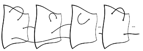
Figure 1: Visualization of the topology fluctuations obtained from the disorder-averaged free energy of the model.

A link with condensed matter physics is almost trivial. A disordered system at low temperatures, or for an anisotropic disorder leads to a model with the same mathematical structure regarding the nonlocality induced by quantum gravity effects on matter fields. The series in Eq. (8) takes into account all possible configurations of the disorder. However, those configurations are not independent, since the disorder average is taken over the free energy, the generating functional of the connected correlation functions.

This concludes the formulation of the analog model. Physical quantities, such as the dynamic and static structure factors, can be readily computed by using a mean-field approximation to obtain the necessary matter-field correlation functions. We recall that the static structure factor is proportional to the total intensity of light scattered by the fluid [37]. As such, the effects of the disorder-induced nonlocality should leave signals on the scattered light.

In summary, we have proposed an analog model for Euclidean wormholes and topological fluctuation effects in a Riemannian space. We aimed at modeling the effects of a quantum theory of gravitation on a matter field. The idea of modeling the internal degrees of freedom by a random field has logical appeal and historical background. Although we based our derivations using a scalar field, the formalism can be easily adapted to other fields, such as vector and spinor fields.

References

- [1] N. D. Birrell and P. C. W. Davies, Quantum Fields in Curved SpaceCambridge Monographs on Mathematical Physics, Cambridge Monographs on Mathematical Physics (Cambridge Univ. Press, Cambridge, UK, 1984).
- [2] L. H. Ford (1997) arXiv:gr-qc/9707062.
- [3] S. Hollands and R. M. Wald, Phys. Rept. 574 (2015) 1, arXiv:1401.2026 [gr-qc].
- [4] L. H. Ford, Phys. Rev. D 51 (1995) 1692, arXiv:gr-qc/9410047.
- [5] L. H. Ford and N. F. Svaiter, Phys. Rev. D 54 (1996) 2640, arXiv:gr-qc/9604052.
- [6] L. H. Ford and N. F. Svaiter, Phys. Rev. D 56 (1997) 2226, arXiv:gr-qc/9704050.
- [7] G. Krein, G. Menezes and N. F. Svaiter, Phys. Rev. Lett. 105 (2010) 131301, arXiv:1006.3350 [hep-th].
- [8] E. Arias, G. Krein, G. Menezes and N. F. Svaiter, Int. Jour. Mod. Phys. A 27 (2012) 1250129, arXiv:1109.6080 [hep-th].
- [9] C. H. G. Bessa, J. G. Duenas and N. F. Svaiter, Class. Quant. Grav. 29 (2012) 215011, arXiv:1204.0022 [hep-th].
- [10] L. H. Ford, V. A. De Lorenci, G. Menezes and N. F. Svaiter, Annals Phys. 329 (2013) 80, arXiv:1202.3099 [gr-qc].
- [11] E. Arias, C. H. G. Bessa, J. G. Dueñas, G. Menezes and N. F. Svaiter, Int. Jour. Mod. Phys. A 29 (2014) 1450024, arXiv:1307.4749 [hep-th].
- [12] S. B. Giddings (2 2022) arXiv:2202.08292 [hep-th].
- [13] G. C. Wick, Phys. Rev. 96 (1954) 1124.
- [14] J. Schwinger, Proc. Nat. Acad. Sci. 44 (1958) 956.
- [15] T. Nakano, Prog. of Theo. Phys. 21 (1959) 241.
- [16] K. Symanzik, Jour.of Math. Phys. 7 (1966) 510.
- [17] K. Osterwalder and R. Schrader, Commun. Math. Phys. 31 (1973) 83.
- [18] K. Osterwalder and R. Schrader, Commun. Math. Phys. 42 (1975) 281.
- [19] I. M. Gel’fand and A. M. Yaglom, Jour. Math. Phys. 1 (1960) 48.
- [20] S. W. Hawking, Phys. Rev. D 37 (1988) 904.
- [21] S. R. Coleman, Nucl. Phys. B 310 (1988) 643.
- [22] I. R. Klebanov, L. Susskind and T. Banks, Nucl. Phys. B 317 (1989) 665.
- [23] J. Preskill, Nucl. Phys. B 323 (1989) 141.
- [24] N. Engelhardt, S. Fischetti and A. Maloney, Phys. Rev. D 103 (2021) 046021, arXiv:2007.07444 [hep-th].
- [25] S. F. Edwards and P. W. Anderson, Jour. of Phys. F 5 (1975) 965.
- [26] K. Okuyama, JHEP 03 (2021) 1, arXiv:2101.05990.
- [27] X. Dong, Nature Commun. 7 (2016) 12472, arXiv:1601.06788 [hep-th].
- [28] T. R. Kirkpatrick and D. Belitz, Phys. Rev. Lett. 76 (1996) 2571, arXiv:cond-mat/9509069.
- [29] D. Belitz, T. R. Kirkpatrick and T. Vojta, Phys.l Rev. B 65 (2002) 165112.
- [30] G. O. Heymans, N. F. Svaiter and G. Krein, Phys. Rev. D 106 (2022) 125004, arXiv:2207.06927 [hep-th].
- [31] S. Sachdev, Quantum Phase Transitions, second edn. (Cambridge University Press, Cambridge, U.K., 2011).
- [32] B. F. Svaiter and N. F. Svaiter, Int. Jour. of Mod. Phys. A 31 (2016) 1650144, arXiv:1603.05919.
- [33] B. F. Svaiter and N. F. Svaiter (2016) [arXiv:1606.04854].
- [34] S. B. Giddings and A. Strominger, Nucl. Phys. B 306 (1988) 890.
- [35] C. D. Dominicis and I. Giardina, Random Fields and Spin Glass (Cambridge University Press, Cambridge, U.K., 2006).
- [36] P. F. González-Díaz, Mod. Phys. Lett. A 8 (1993) 1089.
- [37] J. M. Ortiz de Zárate and J. V. Sengers, Hydrodynamic Fluctuations in Fluids and Fluid Mixtures (Elsevier, Amsterdam, 2006).