Electromagnetic Radiation in chiral matter: the Cherenkov case

Abstract

Starting from the modified Maxwell equations in Carroll-Field-Jackiw electrodynamics we study the electromagnetic radiation in a chiral medium characterized by an axion coupling $\theta(x)=b_{\mu}x^{\mu}$, with $b_{\mu}=(0,\mathbf{b})$, which gives rise to the magnetoelectric effect. Employing the stationary phase approximation we construct the Green’s matrix in the radiation zone which allows the calculation of the corresponding electromagnetic potentials and fields for arbitrary sources. We obtain a general expression for the angular distribution of the radiated energy per unit frequency. As an application we consider a charge moving at constant velocity parallel to $\mathbf{b}$ in the medium and discuss the resulting Cherenkov radiation. We recover the vacuum Cherenkov radiation. For the case of a material with refraction index $n>1$ we find that zero, one or two Cherenkov cones can appear. The spectral distribution of the radiation together with the comparison of the radiation output of each cone are presented, as well as some angular plots showing the appearance of the cones.

I Introduction

Since its experimental discovery in $1934$ cherenkov ; Vavilov , Cherenkov radiation (CHR) has played a fundamental role in the study of the high-energy particle physics, high-power microwave sources and nuclear and cosmic-ray physics Jelley ; Jelley1 , both theoretically and phenomenologically. CHR occurs when charged particles propagate through a dielectric medium with velocity $v$ higher than $c/\sqrt{\epsilon}$, where $c$ is the speed of light in vacuum and $\epsilon$ is the permittivity of the medium, which determines the refractive index $n=\sqrt{\epsilon}$. The first theoretical description of such radiation in the framework of Maxwell’s theory, developed by Frank and Tamm in Ref. FT , reveals its unique directional properties. In particular, CHR is produced in a forward cone defined by the positive angle $\theta=\arccos\left[c/\left(vn\right)\right]$ with respect to the direction of the incident charge. Since the emergence of accelerators in nuclear and high-energy physics CHR has been widely used to design an impressive variety of detectors, such as e.g. the ring-imaging Čerenkov detectors Ypsilantis , which can identify charged particles and also provide a straightforward effective tool to test its physical properties, like velocity, energy, direction of motion and charge PADG . As remarkable cases, one mentions that the anti-proton Chamberlain and the J-particle Aubert were discovered using CHR detectors.

In this paper we deal with CHR in chiral media, which belongs to a class of materials characterized by having a macroscopic electromagnetic response described by non-dynamical axion electrodynamics PECCEI ; SIKIVIE . This is an extension of conventional electrodynamics resulting from the addition of the term $\mathcal{L}_{\theta}=(\alpha/4\pi^{2})\,{\theta}(x)\,(\mathbf{E}\cdot\mathbf{B})$ to the Lagrangian density Wilczek ; Sekine ; Tobar ; Paixao , where $\alpha$ denotes the fine structure constant. Here $\theta(x)$ is a field known as the axion in particle physics which we take as a given parameter of the media in the same footing as the permittivity $\epsilon(x)$ and the permeability $\mu(x)$. Different materials can be characterized according to the choice of $\theta(x)$. For example: (i) magnetoelectric media, that correspond to a non-quantized piecewise constant $\theta(x)$, were discussed in Refs.ODELL ; Kong ; Sihvola ; Bianiso ; Aladadi ; Mahmood ; Lorenci ; Pedro3 ; Urrutia , (ii) topological insulators TI1 ; Urrutia2 ; Maciejko , described by a quantized piecewise constant $\theta(x)$, have been also examined in several applied aspects Chang ; Zou ; Lakhtakia ; Winder ; Li ; Li1 ; Ohnoutek ; Liang ; Tse , (iii) chiral media, including Weyl semimetals, for instance, which display $\theta(x)=b_{\mu}x^{\mu}$ ARM ; Landsteiner ; Ruiz ; KDeng ; Throckmorton ; Barnes ; Hosur ; Day-Nandy , and (iv) metamaterials that can realize a synthetic axion response in non-reciprocal artificially designed structures Shaposhnikov ; Prudencio . The main property characterizing these materials is the magnetoelectric effect (MEE) arising from the additional contribution $\mathcal{L}_{\theta}$ QI_SCIENCE . This coupling produces effective field-dependent charges and current densities which allow the generation of an electric (magnetic) polarization due to the presence of a magnetic (electric) field, even in the static case. Such phenomena were also investigated in the context of the chiral magnetic effect (CME) Kharzeev1 ; Kharzeev1B ; Fukushima ; LiKharzeev ; Vilenkin ; Inghirami ; Chang2 ; Wurff , which brings about the magnetic current density $\mathbf{J}_{B}=\sigma_{B}\mathbf{B}$, with $\sigma_{B}$ playing the role of the magnetic conductivity. Classical repercussions arising from the presence of this current in a dielectric medium were also examined considering symmetric and antisymmetric tensor conductivities Pedro1 , with the antisymmetric tensor conductivity further investigated in Ref. Kaushik1 .

A recently discovered new phenomenon in naturally existing magnetoelectric materials with piecewise constant $\theta(x)$ is the emission of CHR in the backward direction with respect to the incident particle PRDOJF . This remarkable theoretical prediction is analogue to what occurs in left-handed media (LHM), non-natural materials having simultaneously a negative permittivity and permeability, first examined by Veselago Veselago . As these materials, also called metamaterials, are not readily available in nature, they have been artificially constructed and tested in the laboratory Smith-Padilla ; Shelby ; Parazzoli ; Houck ; Kadic ; Engheta ; Pendry ; Pendry2 . Their production has fostered the investigations in backward Cherenkov radiation LU ; Luo ; RRCR ; Sheng ; Chen ; Duan ; Tao .

After integration by parts, the contribution ${\cal L}_{\theta}$ of axion-ED with $\theta(x)=b_{\mu}x^{\mu}$ reduces to the $k_{AF}^{\mu}\sim b^{\mu}$ term of the CTP-odd contribution of the photon sector in the Standard Model Extension (SME) KOSTELECKY , which describes Lorentz invariance violation (LIV) in high energy physics. In this form the theory is also known as the Carroll-Field-Jackiw (CFJ) electrodynamics CFJ . Here, the vector $b^{\mu}$ is introduced either as an explicit Lorentz violating parameter or as the result of the spontaneous Lorentz symmetry breaking of a more fundamental theory. The dynamics induced by the addition of ${\cal L}_{\theta}$ on the usual Maxwell Lagrangian density can be also understood as defining a particular case of electrodynamics in a medium characterized by the generalized constitutive relations, $\mathbf{D}=\mathbf{E}-(\alpha\theta(x)/\pi){\mathbf{B}}$ and $\mathbf{H}=\mathbf{B}+(\alpha\theta(x)/\pi){\mathbf{E}}$, in the case when $\epsilon=1=\mu$.

It is interesting to remark that the CFJ electrodynamics provides an effective theory for condensed-matter systems, accounting for the anomalous Hall effect, the CME, and the electromagnetic response of Weyl semimetals Yan:2016euz , which also constitute a typical representative of chiral matter. In the latter case one finds that the parameters $b_{0}$ and ${\mathbf{b}}$ denote the shift in energy and momentum, respectively, of the two Weyl nodes characterizing the material in the Brillouin zone BURKOV ; FRANZ . Our $b_{\mu}$ differs by a factor of two from that in Ref. FRANZ . Contrary to the case of LIV in high energy physics, all LIV parameters in condensed matter physics arise from the microscopic theory describing the material, thus been well defined and not necessarily suppressed from an experimental perspective.

Vacuum Cherenkov radiation (VCHR) with $n=1$ was discovered in CPT-odd Lorentz-violating theories POTTING1 ; POTTING2 and further extended to the CPT-even sector of the SME ALTSCHUL1 ; ALTSCHUL2 . Reference ALTSCHUL1 puts forward the idea that, besides its description as a conventional radiation process in electrodynamics, CHR can be studied from the matter point of view as the decay, $e^{-}\rightarrow e^{-}+\gamma$, for an arbitrary charge denoted here by $e^{-}$. The latter approach was used to study VCHR for all the Lorentz-violating couplings of fermions that are described by the minimal SME, in the cases with and without spin flip of the fermion MARCO . A complete list of references summarizing previous works on this topic is also found in this paper. The matter approach provides a natural way to find subsequent quantum corrections to the process SCHWINGER and it was used to discuss Cherenkov radiation in the standard vacuum under the influence of strong electromagnetic fields MACLEOD , like those produced by strong laser pulses or in the magnetic field around a pulsar.

Further, a fast charged particle passing from a chiral matter to the vacuum emits transition radiation. Using the matter approach, the photon radiation, $e^{-}\rightarrow e^{-}+\gamma$, and the pair creation, $\gamma\rightarrow e^{+}+e^{-}$, were studied at the boundary between chiral matter and the vacuum TUCHIN1 . Also the ultra-relativistic limit for the case of one infinite domain of chiral matter, together with the case of two semi-infinite domains separated by a domain wall was considered in Ref. TUCHIN2 . The main features of the radiation were shown to depend on the parameters of the chiral anomaly in these materials. Also the high energy limit of the frequency spectrum and the angular distribution for Cherenkov radiation in chiral matter was obtained TUCHIN3 . Anomalous scattering of fermions in matter induced by the chiral anomaly was also investigated, concluding that the scattering angles are proportional to the chiral conductivity TUCHIN4 . Recent studies on collisional energy loss and bremsstrahlung in chiral medium have also been reported with great interest JHansen .

Our discussion of the CHR in a chiral media parallels the analysis of radiation by charged particles described in regular references of electrodynamics Schwinger ; JACKSON ; Panofsky . We obtain a general formula for the radiation fields produced by arbitrary sources, which can be subsequently used to determine all the relevant observable quantities in the radiation processes. As an application of these general findings we next concentrate in CHR, i.e. we consider a charge $q$ moving at constant velocity in the medium, ${|\mathbf{v}|>c/n}$, and neglect recoil effects. We do not restrict ourselves to the ultra high energy limit, thus allowing to address the whole range of (charge) velocities, $|{\mathbf{v}}|/n<|{\mathbf{v}}|<c$. Also, we consider a material with $b_{0}=0$ and choose the charge velocity parallel to ${\mathbf{b}}$, in such a way to assure axial symmetry in our model.

The paper is organized as follows. In section II we summarize the main aspects of CFJ electrodynamics which we use in the following. Section III is devoted to the construction of the Green’s function (GF) of the system in momentum and coordinate space. To this end we further extend to the time-dependent case the methods already developed in Refs. Ruiz ; UrrutiaMartinCambiaso3 ; UrrutiaMartinCambiaso ; UrrutiaMartinCambiaso4 for the static case. In section IV we adopt the stationary phase approximation to calculate the GF in the radiation zone. To make the subsequent calculations still analytic we have to introduce a further approximation in the solution of the stationary phase equation, which determines the range of validity in our calculations that must be verified after obtaining the final results. The resulting electromagnetic fields in the radiation zone are presented in section V for an arbitrary current $J^{\mu}$. Our calculations up to section V together with the Apendixes A, B and C are for $n=1$. An arbitrary index of refraction $n$ is introduced in sections VI and VII following the transformations indicated in the Appendix D. In section VI we consider the particular case of CHR and we calculate the electromagnetic fields, the angular distribution of the radiated energy per unit frequency, the Cherenkov angles and their behavior as a function of the parameter $|{\mathbf{b}}|$. The total radiated power per unit frequency is discussed in section VII, where the ratio between the radiation output of the two possible cones in chiral matter is calculated, as well as the ratio of the production of each of them with respect to the conventional case. Section VIII contains the summary and conclusions. Besides the Appendix D already mentioned, the details of the calculation of the GF for $n=1$ in the radiation zone are summarized in the Appendix A. A general expression for the spectral distribution of the radiation for arbitrary sources and $n=1$ is obtained in the Appendix B, which also summarizes the symmetry properties of some auxiliary functions introduced in the text. The main steps in the calculation for the spectral distribution in the particular case of CHR is presented in the Appendix C for $n=1$. Let us emphasize again that any result obtained for $n=1$ can be generalized to arbitrary $n$ following the prescriptions indicated in the Appendix D.

II CFJ Electrodynamics

In terms of the electromagnetic potential, $A_{\mu}=(\Phi,-\mathbf{A})$, the action is

$$S[A_{\mu}(x)]=\int d^{4}x\left[-\frac{1}{16\pi}F_{\mu\nu}F^{\mu\nu}-\frac{1}{c}J^{\mu}A_{\mu}-\frac{\alpha}{16\pi^{2}}{\theta}(x)F_{\mu\nu}\tilde{F}^{\mu\nu}\right],$$ (1)

where $F_{\mu\nu}=\partial_{\mu}A_{\nu}-\partial_{\nu}A_{\mu}$ and $\tilde{F}^{\mu\nu}=\frac{1}{2}\epsilon^{\mu\nu\rho\sigma}F_{\rho\sigma}$ are the electromagnetic field strength and its dual tensor, respectively, $J^{\mu}=(c\rho,{\mathbf{J}})$ is a conserved external current while $\theta(x)=b_{\mu}x^{\mu}$ is the axion coupling. As usual, the electromagnetic fields are

$$\mathbf{B}=\mbox{\boldmath$\nabla$}\times\mathbf{A},\qquad\mathbf{E}=-\mbox{\boldmath$\nabla$}A^{0}-\frac{1}{c}\frac{\partial\mathbf{A}}{\partial t}.$$ (2)

Our metric is $\eta^{\mu\nu}=\mathrm{diag}(1,-1,-1,-1)$, we set $\epsilon^{0123}=+1$ and employ the unrationalized Gaussian units, following the conventions of Ref. JACKSON .

For a general axion field $\theta(x)$ the action (1) violates translation invariance and Lorentz symmetry KOSTELECKY , but it is manifestly gauge invariant. Nevertheless, in the particular case considered where $b_{\mu}$ is a constant vector, we still have translational invariance. In fact, under the translation, $x^{\mu}\rightarrow x^{\mu}+a^{\mu}$ the additional term proportional to $(b_{\mu}a^{\mu})F_{\mu\nu}{\tilde{F}}^{\mu\nu}$ appears in the action (1). Recalling that $F_{\mu\nu}{\tilde{F}}^{\mu\nu}$ is a total derivative, the invariance of the action under translations is thus recovered. An equivalent way to verify the invariance under translations is integrating by parts the last term in Eq.(1), which produces the Carroll-Field-Jackiw electrodynamics CFJ ,

$$S_{MCFJ}=\int d^{4}x\left[-\frac{1}{16\pi}F_{\mu\nu}F^{\mu\nu}-\frac{1}{c}J^{\mu}A_{\mu}+\frac{\alpha}{16\pi^{2}}b_{\mu}A_{\nu}\tilde{F}^{\mu\nu}\right],$$ (3)

where the translation invariance is manifest and the gauge invariance is granted only up to a total derivative, however. As expected, the resulting equations of motion are gauge invariant, being

$$\partial_{\mu}F^{\mu\nu}=\frac{4\pi}{c}J^{\nu}-{\tilde{b}}_{\mu}\tilde{F}^{\mu\nu},\qquad{\tilde{b}}_{\mu}=\frac{\alpha}{\pi}b_{\mu},$$ (4)

which read

$$[\eta^{\mu\nu}\partial^{2}-\partial^{\mu}\partial^{\nu}-\epsilon^{\mu\nu\rho\sigma}{\tilde{b}}_{\rho}\partial_{\sigma}]A_{\nu}=J^{\mu},$$ (5)

in terms of the potential. The inhomogeneous Maxwell’s equations are

$$\mbox{\boldmath$\nabla$}\cdot\mathbf{E}=4\pi\rho-\mbox{\boldmath$\tilde{b}$}\cdot\mathbf{B},\qquad\mbox{\boldmath$\nabla$}\times\mathbf{B}-\frac{1}{c}\frac{\partial\mathbf{E}}{\partial t}=\frac{4\pi}{c}\mathbf{J}+{\tilde{b}}_{0}\mathbf{B}+\mbox{\boldmath$\tilde{b}$}\times\mathbf{E}.$$ (6)

We still have the homogeneous Maxwell equations arising from the Bianchi identity, $\partial_{\mu}\tilde{F}^{\mu\nu}=0$,

$$\mbox{\boldmath$\nabla$}\cdot\mathbf{B}=0,\qquad\mbox{\boldmath$\nabla$}\times\mathbf{E}+\frac{1}{c}\frac{\partial\mathbf{B}}{\partial t}=0.$$ (7)

In Eqs. (6) we have $\mbox{\boldmath$\tilde{b}$}=\mathbf{\nabla}\theta$ and ${\tilde{b}}_{0}=\partial_{t}\theta$, where $\theta$ is the axion field. The terms involving derivatives of $\theta$ play relevant roles in condensed matter systems ZQ ; Pedroo . Indeed, while $\mathbf{\nabla}\theta\cdot\mathbf{B}$ represents an anomalous charge density, $\mathbf{\nabla}\theta\times\mathbf{B}$ appears in the anomalous Hall effect (AHE) and $(\partial_{t}\theta)\mathbf{B}$ stands for the chiral magnetic current Kharzeev1 ; Kharzeev1B ; Fukushima ; LiKharzeev ; Vilenkin ; Inghirami ; Chang2 ; Wurff ; Pedro1 ; Kaushik1 . In the case when the axion field does not depend on the space coordinates, $\mathbf{\nabla}\theta={\bf{0}},$ the Maxwell equations (6) read

$$\mathbf{\nabla}\cdot\mathbf{E}=4\pi\rho,\qquad\mathbf{\nabla}\times\mathbf{B}-\frac{1}{c}\frac{\partial\mathbf{E}}{\partial t}=\frac{4\pi}{c}\mathbf{J}+(\partial_{t}\theta)\mathbf{B},$$ (8)

with $\partial_{t}\theta$ representing the magnetic conductivity, $\sigma_{B}$, in the chiral current, $\mathbf{J}_{B}=\sigma_{B}\mathbf{B}$. Effects of the CFJ term, together with those arising from its higher derivative dimension five counterpart, on the electromagnetic propagation in continuous matter were analyzed from a classical perspective in Ref. Pedroo .

Since our main interest is in radiation processes, we look for the energy density ${{\bar{u}}}$ and the energy flux $\mathbf{\ {\bar{S}}}\,$ satisfying the conservation equation $\partial_{t}{\bar{u}}+\mbox{\boldmath$\nabla$}\cdot{\mathbf{\bar{S}}}=0$ outside the sources. From the standard manipulations of Maxwell’s equations (6) and (7) we obtain

$$-{\mathbf{J}}\cdot{\mathbf{E}}=\frac{\partial u}{\partial t}+\mbox{\boldmath$\mbox{\boldmath$\nabla$}$}\cdot\mathbf{\ S}+\frac{c}{4\pi}\tilde{b}_{0}(\mathbf{E}\cdot\mathbf{B}),$$ (9)

with

$${u}=\frac{1}{8\pi}\Big{(}\mathbf{E}^{2}+\mathbf{B}^{2}\Big{)},\qquad\mathbf{S}=\frac{c}{4\pi}\mathbf{E}\times\mathbf{B}.$$ (10)

The identity

$$\mathbf{E}\cdot\mathbf{B}=-\frac{1}{2c}\frac{\partial}{\partial t}(\mathbf{A}\cdot\mathbf{B})+\frac{1}{2}\mbox{\boldmath$\nabla$}\cdot(\mathbf{A}\times\mathbf{E}-A^{0}\mathbf{B}),$$ (11)

allows us to define the energy density $\bar{u}$, together with the corresponding Poynting vector $\mathbf{\bar{S}}$, as

$${\bar{u}}=u-\frac{1}{8\pi}{\tilde{b}}_{0}\mathbf{A}\cdot{\mathbf{B}},\qquad\mathbf{\bar{S}}=\mathbf{S}+\frac{1}{8\pi}{\tilde{b}}_{0}(\mathbf{A}\times\mathbf{E}-A^{0}\mathbf{B}),$$ (12)

fulfilling the required conservation equation when ${\mathbf{J}}=0$. Similar results are obtained from the covariant version of the energy-momentum tensor in Refs. CFJ ; POTTING1 ; POTTING2 , which confirms $\bar{u}$ and $\bar{S}$, given in Eq. (12), as the energy density and and energy flux that respect the continuity equation.

Let us emphasize that under the gauge transformation, $\delta_{\Lambda}A^{0}=\frac{1}{c}\frac{\partial\delta\Lambda}{\partial t},\,\delta_{\Lambda}\mathbf{A}=-\mbox{\boldmath$\nabla$}\delta\Lambda$, the terms that depend on the potential $A^{\mu}$ in Eq. (12) are gauge invariant up to a total derivative, changing as

$$\delta_{\Lambda}(\mathbf{A}\cdot\mathbf{B})=\Lambda\mbox{\boldmath$\nabla$}\cdot\mathbf{B},\qquad\delta_{\Lambda}(\mathbf{A}\times\mathbf{E}-A^{0}\mathbf{B})=\lambda\left(\mbox{\boldmath$\nabla$}\times\mathbf{E}-\frac{1}{c}\frac{\partial\mathbf{B}}{\partial t}\right),$$ (13)

which yield null results when one takes into account the homogeneous Maxwell equations. From Eq. (12) we realize that $\bar{u}$ is not positive definite, which prompts us to set $b_{0}=0$ in the following to avoid instabilities in the system ZQ . Also, we take the $z$-axis in the direction of the $\mathbf{b}$ vector

III The Green’s function

III.1 Green’s function in momentum space

Our next step is to construct the Green function (GF) $G_{\mu\nu}(x-x^{\prime})$ of CFJ electrodynamics in the time dependent case. It is defined by

$$[\eta^{\mu\nu}\partial^{2}-\partial^{\mu}\partial^{\nu}-{\tilde{b}}_{\rho}\epsilon^{\mu\nu\rho\sigma}\partial_{\sigma}]G_{\nu\beta}(x-x^{\prime})=\delta^{\nu}{}_{\beta}\delta^{4}(x-x^{\prime}).$$ (14)

Going to momentum space, we write

$$G_{\nu\beta}(x-x^{\prime})=\int\frac{d^{4}k}{(2\pi)^{4}}e^{-ik_{\mu}{(x-x^{\prime})^{\mu}}}G_{\nu\beta}(\omega,\mathbf{k}),\quad x^{\mu}=(ct,\mathbf{x}),\quad k^{\mu}=(\omega/c,\mathbf{k}),\quad\partial_{\mu}=-ik_{\mu},$$ (15)

obtaining

$$[-k^{2}\eta^{\mu\nu}+k^{\mu}k^{\nu}+i\epsilon^{\mu\nu\rho\sigma}{\tilde{b}}_{\rho}k_{\sigma}]G_{\nu\beta}(k)=\delta^{\mu}{}_{\beta},$$ (16)

which in the Lorentz gauge, $\partial_{\mu}A^{\mu}=0$, reduces to

$$[-k^{2}\eta^{\mu\nu}+i\epsilon^{\mu\nu\rho\sigma}{\tilde{b}}_{\rho}k_{\sigma}]G_{\nu\beta}(k)=\delta^{\mu}{}_{\beta},$$ (17)

with $k^{2}=k_{0}^{2}-\mathbf{k}^{2}$. A long but straightforward calculation yields

$$G_{\nu\lambda}(k)=-\frac{k^{2}\eta_{\nu\lambda}+{\tilde{b}}_{\nu}{\tilde{b}}_{\lambda}+i\epsilon_{\nu\lambda\alpha\beta}{\tilde{b}}^{\alpha}k^{\beta}}{k^{4}+{\tilde{b}}^{2}k^{2}-({\tilde{b}}\cdot k)^{2}}+\frac{({\tilde{b}}\cdot k)({\tilde{b}}_{\lambda}k_{\nu}+{\tilde{b}}_{\nu}k_{\lambda})-{\tilde{b}}^{2}k_{\nu}k_{\lambda}}{k^{2}(k^{4}-{\tilde{b}}^{2}k^{2}+({\tilde{b}}\cdot k)^{2})}.$$ (18)

At this stage we can verify that $k^{\nu}G_{\nu\lambda}(k)=0$. The above expression can be further simplified recalling the relation $A_{\nu}(k)=G_{\nu\lambda}(k)J^{\lambda}(k)$. Since $G_{\nu\lambda}(k)$ couples to a conserved current, we can dispose of all factors proportional to $k_{\lambda}J^{\lambda}$. Furthermore, note that any contribution proportional to $k_{\nu}$ corresponds to a gauge transformation in the resulting $A_{\nu}$. Then, a simpler representation of the function (18), without loss of generality, is

$$G_{\nu\lambda}=-\frac{k^{2}\eta_{\nu\lambda}+{\tilde{b}}_{\nu}{\tilde{b}}_{\lambda}+i\epsilon_{\nu\lambda\alpha\beta}{\tilde{b}}^{\alpha}k^{\beta}}{k^{4}+{\tilde{b}}^{2}k^{2}-({\tilde{b}}\cdot k)^{2}},$$ (19)

coinciding with the result of Refs. POTTING1 ; POTTING2 ; ZQ , but no longer written in the Lorenz gauge.

III.2 Green’s function in coordinate space

In order to deal with radiation, we need to express the GF in the coordinate space. To this end, we keep the dependence on the frequency and perform the Fourier transform only in coordinate space. We set ${\tilde{b}}_{\mu}=(0,0,0,b),$ with $b=|\mbox{\boldmath$\tilde{b}$}|=\alpha|\mathbf{b}|/\pi$. Starting from Eq. (19), we write

$$G^{\mu\nu}(\mathbf{x},\mathbf{x^{\prime}};\omega) = \int\frac{d^{3}k}{(2\pi)^{3}}G^{\mu\nu}(\omega,\mathbf{k})e^{i\mathbf{k}\cdot(\mathbf{x}-\mathbf{x^{\prime}})},$$

$$G^{\mu\nu}(\mathbf{x},\mathbf{x^{\prime}};\omega) = -\int\frac{d^{3}k}{(2\pi)^{3}}\frac{k^{2}g^{\mu\nu}+ib\epsilon^{\mu\nu 3\sigma}k_{\sigma}+{{\tilde{b}}}^{\mu}{{\tilde{b}}}^{\nu}}{(k^{2})^{2}+{{\tilde{b}}}^{2}k^{2}-({{\tilde{b}}}\cdot k)^{2}}e^{i\mathbf{k}\cdot(\mathbf{x}-\mathbf{x^{\prime}})},$$

$$G^{\mu\nu}(\mathbf{x},\mathbf{x^{\prime}};\omega) = -\left[(k_{0}^{2}+\mbox{\boldmath$\nabla$}^{2})g^{\mu\nu}+ik_{0}b\epsilon^{\mu\nu 30}-b\epsilon^{\mu\nu 3i}\partial_{i}+{\tilde{b}}^{\mu}{\tilde{b}}^{\nu}\right]f(\mathbf{x},\mathbf{x^{\prime}};\omega),$$ (20)

in terms of $\partial_{j}=-ik_{j}$, and introduce the function,

$$f(\mathbf{x},\mathbf{x^{\prime}};\omega)=\int\frac{d^{3}k}{(2\pi)^{3}}\frac{e^{i\mathbf{k}\cdot(\mathbf{x}-\mathbf{x^{\prime}})}}{(k^{2})^{2}+{\tilde{b}}^{2}k^{2}-({\tilde{b}}\cdot k)^{2}},$$ (21)

from which we calculate the Green’s function according to Eq. (20). Under our conventions, the denominator in Eq. (21) is

$$D\equiv(k^{2})^{2}+\tilde{b}^{2}k^{2}-(\tilde{b}\cdot k)^{2}=(k_{0}^{2}-\mathbf{k}^{2})^{2}-b^{2}(k_{0}^{2}-\mathbf{k}^{2})-b^{2}k_{3}^{2}.$$ (22)

The condition $D=0$ yields the dispersion relation

$$k_{0}^{2}=k_{\perp}^{2}+\left(\sqrt{k_{z}^{2}+b^{2}/4}\pm b/2\right)^{2},$$ (23)

where

$${\mathbf{k}}^{2}=k_{\perp}^{2}+k_{z}^{2},\quad k_{\perp}=+\sqrt{k_{x}^{2}+k_{y}^{2}}.$$ (24)

Setting $b=0$ in the dispersion relation (23), one recovers the conventional vacuum result.

The evaluation of Eq. (21) is performed in cylindrical coordinates using the integration over the polar angle to introduce the Bessel function $J_{0}$ and, subsequently, calculating the integral over $k_{z}$ in the complex plane. To this end, we rewrite the denominator $D$ as

$$D=\left(k_{z}^{2}-(k_{z}^{-})^{2}\right)\left(k_{z}^{2}-(k_{z}^{+})^{2}\right),$$ (25)

which allows the identification of the poles in $k_{z}$,

$$k_{z}^{\pm}=\sqrt{k_{\parallel}^{2}\pm bk_{\parallel}},$$ (26)

with the redefinition,

$$k_{\parallel}=\sqrt{k_{0}^{2}-k_{\perp}^{2}}.$$ (27)

The integration over $k_{z}$ is long but straightforward, yielding the final result

$$f(\mathbf{x},\mathbf{x^{\prime}};\omega)=\frac{i}{8\pi}\int_{0}^{\infty}\frac{k_{\perp}\,dk_{\perp}}{k_{\parallel}}\,J_{0}\Big{(}R_{\perp}k_{\perp}\Big{)}\frac{1}{b}\left[\frac{e^{i\sqrt{k_{\parallel}^{2}+bk_{\parallel}}Z}}{\sqrt{k_{\parallel}^{2}+bk_{\parallel}}}-\frac{e^{i\sqrt{k_{\parallel}^{2}-bk_{\parallel}}Z}}{\sqrt{k_{\parallel}^{2}-bk_{\parallel}}}\right],$$ (28)

where we stick to our independent variable $k_{\perp}>0$ and define $Z=|z-z^{\prime}|$. Setting $k_{0}=0$, we recover the static approximation considered in Ref. ZQ .

IV The Green’s function in the radiation zone

The relations, $J_{0}(x)=(H_{0}^{(1)}(x)+(H_{0}^{(2)}(x))/2$ and $H_{0}^{(1)}(e^{i\pi}x)=-H_{0}^{(2)}(x)$, allow to extend the integration limit of $k_{\perp}$ from $-\infty$ to $+\infty$, yielding the convenient expression

$$f(\mathbf{x},\mathbf{x^{\prime}};\omega)=\sum_{\eta=\pm 1}f_{\eta}(\mathbf{x},\mathbf{x^{\prime}};\omega),\quad f_{\eta}(\mathbf{x},\mathbf{x^{\prime}};\omega)=\frac{i}{16\pi}\int_{-\infty}^{\infty}\frac{k_{\perp}\,dk_{\perp}}{k_{\parallel}}\,H_{0}^{(1)}\Big{(}k_{\perp}R_{\perp}\Big{)}\frac{1}{\eta b}\frac{e^{i\sqrt{k_{\parallel}^{2}+\eta b\,k_{\parallel}}Z}}{\sqrt{k_{\parallel}^{2}+\eta b\,k_{\parallel}}},$$ (29)

with $b>0$ everywhere, and the sum on $\eta=\pm 1$ contemplates the two square roots present in Eq. (28). The extension to the complex plane of the integral on the variable $k_{\perp}$ is made by introducing the Sommerfeld path, shown schematically in Fig. 1.

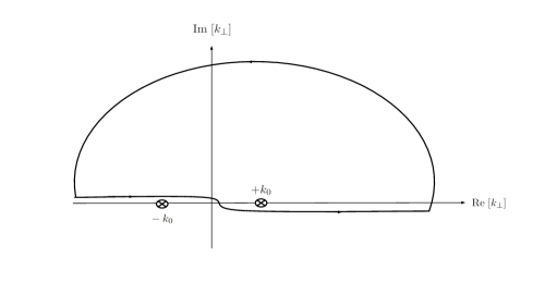
Figure 1: The Sommerfeld integration path. The path is above the logarithmic branch point singularity of $H_{0}^{(1)}(K_{\perp}R_{\perp})$ at $k_{\perp}=0$. Furthermore $k_{\parallel}=\sqrt{k_{0}^{2}-k_{\perp}^{2}}$ has singularities at $k_{\perp}=\pm k_{0}$.

In the following we concentrate upon the calculation of $f_{\eta}(\mathbf{x},\mathbf{x^{\prime}};\omega)$ in the far-zone regime, $r=|{\mathbf{x}}|\gg|{\mathbf{x^{\prime}}}|=r^{\prime}$, where we have highly oscillating functions in the integrand of Eq. (29). This property suggests the use of the stationary phase approximation (SPA) to evaluate the integral. We consider the approximation $R_{\perp}=|(\mathbf{x}-\mathbf{x^{\prime})}_{\perp}|=R|\sin\theta|$, together with $Z=|x_{3}-x_{3}^{\prime}|=R|\cos\theta|$, where $R=|(\mathbf{x}-\mathbf{x^{\prime})}|$ and $\theta$ is the polar angle of the observation point determined by $\mathbf{x}$. To assess the validity of the approximation we have to compare the directions of the vectors $\mathbf{x}$ and $\mathbf{R}=\mathbf{(x-x^{\prime})}$, with respect to the $z$-axis. In the most unfavorable situation, when $\mathbf{x^{\prime}}$ is orthogonal to $\mathbf{x}$, we can show that the angle $\Theta$ that the vector ($\mathbf{x}-\mathbf{x^{\prime}}$) makes with the $z$-axis is such that $\cos\Theta=\cos\theta-(r^{\prime}/r)\sin\theta$, to first order in $r^{\prime}/r$. That is to say, it is a very good approximation to take $\Theta\approx\theta$ in the regime $r^{\prime}/r\ll 1$. This, together with the asymptotic behavior

$$H_{0}^{(1)}(k_{\perp}R_{\perp})=\sqrt{\frac{2}{\pi k_{\perp}R_{\perp}}}e^{ik_{\perp}R_{\perp}-i\pi/4},$$ (30)

yields

$$f_{\eta}(\mathbf{x},\mathbf{x^{\prime}};\omega)=\frac{ie^{-i\pi/4}}{16\pi}\sqrt{\frac{2}{\pi}}\int_{-\infty}^{\infty}\frac{k_{\perp}\,dk_{\perp}}{k_{\parallel}}\,\frac{1}{\sqrt{k_{\perp}r\sin\theta}}\frac{1}{\eta b}\frac{e^{iR\left(k_{\perp}|\sin\theta|+\sqrt{k_{\parallel}^{2}+\eta b\,k_{\parallel}}|\cos\theta|\right)}}{\sqrt{k_{\parallel}^{2}+\eta b\,k_{\parallel}}}.$$ (31)

As usual, we further replace $R$ by $r$, except in the phase of the exponential, where we assume $R=\left(r-\hat{\mathbf{n}}\cdot\mathbf{x^{\prime}}\right)$, with $\mathbf{\hat{n}}=\mathbf{x}/r$, thus taking into account the phase modifications induced by the source.

We recall the general expression for the SPA

$$I=\int_{-\infty}^{+\infty}\,dt\,e^{iR\,h(t)}\,f(t)=e^{iR\,h(t_{0})}\,f(t_{0})\,\sqrt{\frac{2\pi i}{rh^{\prime\prime}(t_{0})}},$$ (32)

where $R\gg 1$ and $t_{0}$ is the solution of $h^{\prime}(t)=0$, which makes $h^{\prime}(t_{0})$ an extremum of $h(t).$ The prime (^′) denotes the derivatives with respect to $t$ in the usual fashion. The functions $h(t)$ and $f(t)$ are identified by comparing with those in Eq. (31) after the far field approximation is imposed. In Eq. (31), we choose to find the stationary phase by looking at the extreme of the functions,

$$h_{\eta}(k_{\perp})=k_{\perp}|\sin\theta|+\,\sqrt{k_{\parallel}^{2}+\eta b\,k_{\parallel}}\,|\cos\theta|>0.$$ (33)

To this end, we take the derivative of $h_{\eta}$ with respect to $k_{\parallel}$ for simplicity. Since $dk_{\parallel}/dk_{\perp}\neq 0$ and the resulting relation is set equal to zero, the outcome is independent of the variable chosen to calculate the derivative. After rearranging the result of $dh_{\eta}(k_{\perp})/dk_{\parallel}$, we find it convenient to present the condition for the extremum as

$${\frac{\kappa}{\sqrt{1-\kappa^{2}}}\tan\theta}=\left(1+\frac{\eta}{2}\frac{\beta}{\kappa}\right)\left(1+\eta\frac{\beta}{\kappa}\right)^{-1/2},$$ (34)

in terms of the dimensionless variables $\kappa$ and $\beta$, defined as

$$\kappa=\frac{k_{\parallel}}{k_{0}}>0,\qquad\beta=\frac{b}{k_{0}}>0.$$ (35)

The Eq. (34) is a quartic equation for $\kappa$ which is difficult to solve analytically. For a given $\beta$, the exact numerical solution $\kappa(\theta)$ of Eq. (34) is indicated with the dashed (red) line for $\eta=+1$ and with de dotted (blue) line for $\eta=-1$, in the panels of Fig. 2. To proceed further we resort to an approximation in the solution of Eq. (34) considering the limit $b\ll k_{\parallel}<k_{0}$, where $\beta/\kappa\ll 1$. Then, Eq. (34) simplifies as

$$\frac{\kappa^{2}}{1-\kappa^{2}}\tan^{2}\theta=1+{\frac{1}{4}}\left(\frac{\beta}{\kappa}\right)^{2}+O(\beta^{3}).$$ (36)

To first order in ${\beta}/{\kappa}$, we obtain $\kappa=\cos\theta$ as our approximate SPA solution, for each value of $\eta$. This choice yields

$$k_{\parallel}(\theta,\eta)=k_{0}|\cos\theta|,\qquad k_{\perp}(\theta,\eta)=k_{0}|\sin\theta|.$$ (37)

The solution (37), called the classical SPA, is plotted as the solid (magenta) line in Fig. 2. Let us emphasize that this approximation is taken only to have a simpler analytic way to proceed with the calculation and that $b,(\beta)$, is taken non-zero in all the required remaining functions. The approximation is valid whenever $\cos\theta\gg\beta/(2\sqrt{2})$, which should be verified at the end of any determination of a Cherenkov angle. In any case, Figs. 2 provide a qualitative idea of the validity of the approximation (37), showing that it is very good for the contribution $\eta=+1$ in the whole angular range. Looking back to Eq. (29) we realize that this is not the case for the contribution $\eta=-1$, which is suppressed to the right of the vertical (green) line shown in the figures, where $\sqrt{k^{2}_{\parallel}-bk_{\parallel}}$ becomes imaginary. This line corresponds to $\theta_{0}=\arccos\beta$.

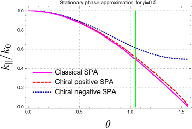
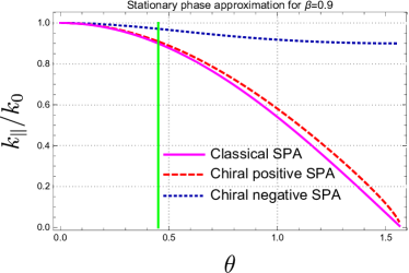
Figure 2: The exact numerical solution $\kappa(\theta)$ of Eq. (34) is indicated with the dashed (red) line for $\eta=+1$ and with the dotted (blue) line for $\eta=-1$. The solution $\kappa(\theta)$ of the approximation in Eq. (37), called classical SPA, is plotted as a solid (magenta) line. The vertical solid (green) line indicates the angle $\theta=\arccos\alpha$, to the right of which $\sqrt{k^{2}_{\parallel}-bk_{\parallel}}$ becomes imaginary. Left panel: $\beta=0.5$. Right panel: $\beta=0.9$

Recalling Eqs. (31) and (32), and substituting the SPA (37), we arrive at

$$f(\mathbf{x},\mathbf{x^{\prime}};\omega)|_{\rm SPA}\equiv\mathfrak{f}(\mathbf{x},\mathbf{x^{\prime}};\omega),$$

$$\mathfrak{f}(\mathbf{x},\mathbf{x^{\prime}};\omega)=\frac{1}{8\pi r}\frac{1}{k_{0}\,b|\cos\theta|}\sum_{\eta=\pm 1}\frac{e^{ik_{0}C_{\eta}(\theta)(r-\mathbf{\hat{n}}\cdot\mathbf{x^{\prime}})}}{g_{\eta}(\theta)},$$ (38)

with

$$C_{\eta}(\theta)=\left(\sin^{2}\theta+\cos^{2}\theta\sqrt{1+\eta\beta|\sec\theta|}\right),$$ (39)

$$g_{\eta}(\theta)=\frac{1}{\left(1+\eta\beta|\sec\theta|\right)^{1/4}}\sqrt{\left(1+\eta\beta|\sec\theta|\right)\left(1+\frac{\eta\beta}{2}|\sec\theta|\right)+\frac{\beta^{2}}{4}{\tan^{2}\theta}}.$$ (40)

Let us remark the following obvious symmetry properties in terms of the frequency

$$C_{\eta}(-\omega)=C_{-\eta}(\omega),\qquad g_{\eta}(-\omega)=g_{-\eta}(\omega),$$ (41)

which will be useful in the following. A word of caution is required here. If we had solved the stationary phase equation exactly, any change of variables in the subsequent integration would produce the same result. This is not the case when using an approximation as we have done. Since we have chosen $k_{\perp}$ as our integration variable, we have to make sure that the second derivative $h^{\prime\prime}_{\eta}$ is calculated with respect to $k_{\perp}$. Notice that in the limit $\alpha=0$ we have $C_{\eta}(\theta)=1$, and we recover the phase $ik_{0}R$ describing conventional radiation. Also, $g_{\eta}(\theta)=1$ in that limit.

We choose to split the GF in Eq. (20) as

$$G_{0}^{\mu\nu}(\mathbf{x},\mathbf{x^{\prime}};\omega) = -g^{\mu\nu}(k_{0}^{2}+\mbox{\boldmath$\nabla$}^{2})f(\mathbf{x},\mathbf{x^{\prime}};\omega),$$ (42)

$$G_{b}^{\mu\nu}(\mathbf{x},\mathbf{x^{\prime}};\omega) = -b\left[i\omega\epsilon^{\mu\nu 30}-\epsilon^{\mu\nu 3i}\partial_{i}\right]f(\mathbf{x},\mathbf{x^{\prime}};\omega),$$ (43)

$$G_{b^{2}}^{\mu\nu}(\mathbf{x},\mathbf{x^{\prime}};\omega) = -{\tilde{b}}^{\mu}{\tilde{b}}^{\nu}f(\mathbf{x},\mathbf{x^{\prime}};\omega),$$ (44)

whose evaluation requires the calculation on the action of the operators,

$$\left(k_{0}^{2}+\mbox{\boldmath$\nabla$}^{2}\right)=\left(k_{0}^{2}+\mbox{\boldmath$\nabla$}_{\bot}^{2}+\frac{\partial^{2}}{\partial Z^{2}}\right),$$ (45)

and $\partial_{i}$ on the function $\mathfrak{f}(\mathbf{x},\mathbf{x^{\prime}};\omega)$, which is the far field approximation of $f(\mathbf{x},\mathbf{x^{\prime}};\omega)$. Instead of applying these operators directly on $\mathfrak{f}(\mathbf{x},\mathbf{x^{\prime}};\omega)$, we choose to act upon the exact expressions (29) for $f_{\eta}(\mathbf{x},\mathbf{x^{\prime}};\omega)\;$ and subsequently evaluate the results in terms of the stationary phase proposed previously. The calculation is sketched in the Appendix A, yielding the result

$$G^{\mu\nu}(\mathbf{x},\mathbf{x^{\prime}};\omega)=\frac{1}{8\pi}\sum_{\eta=\pm 1}\frac{e^{ik_{0}C_{\eta}(\theta)r}}{g_{\eta}(\theta)}{H}_{\eta}{}^{\mu\nu}(\mathbf{\hat{n}})\frac{1}{r}\,e^{-ik_{0}\mathbf{\hat{n}}\cdot\mathbf{x^{\prime}}C_{\eta}(\theta)},$$ (46)

with

$${H}_{\eta}{}^{\mu\nu}(\mathbf{\hat{n}})=\begin{pmatrix}1&-i\eta|\tan\theta|\sin\phi&\ i\eta|\tan\theta|\cos\phi&0\\ i\eta|\tan\theta|\sin\phi&-1&\ i\eta|\sec\theta|&0\\ -i\eta|\tan\theta|\cos\phi&\ -i\eta|\sec\theta|&-1&0\\ 0&0&\ 0&-(1+\eta\beta|\sec\theta|).\end{pmatrix},$$ (47)

fulfilling the following symmetry property

$$H_{\eta}{}^{\mu\nu}(-\omega)=(H_{-\eta}{}^{\mu\nu}(\omega))^{*}.$$ (48)

As another check of consistency, let us recover the conventional GF when $\beta=0$. Recalling $C_{\eta}(\theta)=1$ and $g_{\eta}(\theta)=1$ in this case, the GF turns into

$$G^{\mu\nu}(\mathbf{x},\mathbf{x^{\prime}};\omega)=\frac{1}{8\pi}\frac{e^{ik_{0}(r-\mathbf{\hat{n}}\cdot\mathbf{x^{\prime}})}}{r}\sum_{\eta=\pm 1}{H}_{\eta}{}^{\mu\nu}(\mathbf{\hat{n}})=\eta^{\mu\nu}\frac{1}{4\pi}\frac{e^{ik_{0}(r-\mathbf{\hat{n}}\cdot\mathbf{x^{\prime}})}}{r},$$ (49)

since the non-diagonal terms in Eq. (47) cancel in the sum, while those in the diagonal get a factor of two.

V The electromagnetic fields in the radiation zone

In this section we calculate $\mathbf{E}$ and $\mathbf{B}$ in the far-field approximation, for an arbitrary localized current $J_{\nu}(\mathbf{x^{\prime}},\omega)$. We start from the vector potential together with the relation

$$A^{\mu}(\mathbf{x},\omega)=\frac{4\pi}{c}\int d^{3}x^{\prime}\;G^{\mu\nu}(\mathbf{x},\mathbf{x^{\prime}};\omega)\,J_{\nu}(\mathbf{x^{\prime}},\omega),$$ (50)

which, with the GF (46) implemented, yields

$$A^{\mu}(\mathbf{x},\omega)=\frac{1}{2c}\sum_{\eta=\pm 1}\frac{1}{g_{\eta}(\theta)}{H}_{\eta}{}^{\mu\nu}(\mathbf{\hat{n}})\frac{1}{r}e^{ik_{0}C_{\eta}(\theta)r}\int d^{3}x^{\prime}e^{-ik_{0}C_{\eta}(\theta)\hat{\mathbf{n}}\cdot\mathbf{x^{\prime}}}J_{\nu}(\mathbf{x^{\prime}},\omega),$$ (51)

where the only dependence of the GF on the source points $\mathbf{x}{{}^{\prime}}$ is in the exponential $\exp(-ik_{0}\hat{\mathbf{n}}\cdot\mathbf{x^{\prime}}\,C_{\eta}(\theta))$. Thus, the relevant integral is the space Fourier transform

$$\mathcal{J}^{\nu}({}\mathbf{k}{}_{\eta},\,\omega)=\int d^{3}x^{\prime}\,e^{-ik_{0}C_{\eta}(\theta)\hat{\mathbf{n}}\cdot\mathbf{x^{\prime}}}\ J^{\nu}(\mathbf{x^{\prime}},\omega),$$ (52)

with

$$\mathbf{k}{}_{\eta}=\mathbf{\hat{r}}k_{0}C_{\eta}(\theta),\qquad\mathbf{\hat{r}}=(\sin\theta\cos\phi,\,\sin\theta\sin\phi,\,\cos\theta),$$ (53)

where $\theta$ and $\phi$ are the observation angles in spherical coordinates. Let us remark that no absolute values in the $\theta$-dependent angular functions appear in $\mathbf{\hat{r}}$. The electromagnetic potential is then

$$A^{\mu}(\mathbf{x},\omega)=\frac{1}{2c}\sum_{\eta=\pm 1}\frac{1}{g_{\eta}(\theta)}{H}_{\eta}{}^{\mu\nu}(\hat{{\mathbf{r}}})\;{\mathcal{J}}_{\nu}({}\mathbf{k}{}_{\eta},\,\omega)\left(\frac{1}{r}e^{ik_{0}C_{\eta}(\theta)r}\right).$$ (54)

Collecting the symmetry properties given in Eqs. (41) and (48) and using $J^{\mu}(\mathbf{x},-\omega)=(J^{\mu}(\mathbf{x},\omega))^{*}$, we arrive at the relation

$$\qquad A^{\mu}_{\eta}(\mathbf{x},-\omega)=(A^{\mu}_{-\eta}(\mathbf{x},\omega))^{*}.$$ (55)

We can verify again the correct limit $\beta=0$, since now ${\mathbf{k}}_{\eta}={\mathbf{\hat{n}}k_{0}}$ independently of $\eta$, because $C_{\eta}(\theta)=1$, so that the sum in (54) reduces to ${\cal J}_{\nu}\sum_{\eta=\pm 1}H_{\eta}^{\mu\nu}$. As mentioned previously, the off-diagonal terms cancel and those in the diagonal yield $2\eta^{\mu\nu}$. Remember also that $g_{\eta}(\theta)=1$ when $\beta=0$.

To calculate the electromagnetic fields $\mathbf{E}(\mathbf{x},\omega)=ik_{0}\mathbf{A}(\mathbf{x},\omega)-\mbox{\boldmath$\nabla$}A^{0}(\mathbf{x},\omega)$ and $\mathbf{B}(\mathbf{x},\omega)=\mbox{\boldmath$\nabla$}\times\mathbf{A}(\mathbf{x},\omega)$, it is convenient to write the vector potential (54) in the form

$${A}^{\mu}=\sum_{\eta=\pm 1}A^{\mu}_{\eta},\quad A^{\mu}_{\eta}=\mathcal{A}_{\eta}^{\mu}(\theta,\phi)\left(\frac{1}{g_{\eta}(\theta)}\frac{1}{2cr}e^{ik_{0}C_{\eta}(\theta)r}\right),\,\,\,\,\,\mathcal{A}_{\eta}^{\mu}(\theta,\phi)={H}_{\eta}{}^{\mu\nu}(\mathbf{\hat{r}})\;{\mathcal{J}}_{\nu}({}\mathbf{k}{}_{\eta},\,\omega).$$ (56)

As usual, the form of the outgoing wave $\exp(ik_{0}C_{\eta}(\theta)r)/r$ in the radiation zone provides an important simplification when considering the action of the gradient operator. It is a direct calculation to show that

$${\mbox{\boldmath$\nabla$}}\Big{(}U(\theta,\phi)\frac{1}{r}e^{ik_{0}C_{\eta}(\theta)r}\Big{)}=ik_{0}{\mathbf{N}}_{\eta}\Big{(}U(\theta,\phi)\frac{1}{r}e^{ik_{0}C_{\eta}(\theta)r}\Big{)},$$ (57)

for an arbitrary angular function $U(\theta,\phi)$ in the far-field approximation, with

$${\mathbf{N}}_{\eta}=\Big{[}C_{\eta}(\theta)\,\hat{{\mathbf{r}}}+\frac{\partial C_{\eta}(\theta)}{\partial\theta}\,\mbox{\boldmath$\hat{\theta}$}\Big{]}.$$ (58)

In accordance with the expression (57), the equivalence $\mbox{\boldmath$\nabla$}=ik_{0}\mathbf{N}_{\eta}$ holds for the action of $\nabla$ on the function between parentesis in (57), to first order in $1/r$. This is the generalization of the familiar property, $\mbox{\boldmath$\nabla$}\rightarrow ik_{0}\mathbf{\hat{r}}$, in the scenario of conventional radiation. Let us observe that the dependence on $\hat{\theta}$, which is not present in the standard case, arises because the $\theta$-dependent phase factor $C_{\eta}(\theta)$ in the exponential $\exp(ik_{0}C_{\eta}(\theta)r)$. The electromagnetic fields can also be decomposed into their $\eta$-contributions and they are

$${\mathbf{B}}=\sum_{\eta=\pm 1}{\mathbf{B}}_{\eta},\quad{\mathbf{B}}_{\eta}=ik_{0}\big{(}{\mathbf{N}}_{\eta}\times\,\mathbf{A}_{\eta}\big{)},$$ (59)

$${\mathbf{E}}=\sum_{\eta=\pm 1}{\mathbf{E}}_{\eta},\quad{\mathbf{E}}_{\eta}=ik_{0}\Big{(}\mathbf{A}_{\eta}-{\mathbf{N}}_{\eta}\,{A}_{\eta}^{0}\Big{)},$$ (60)

where we recall that the expression of the vector potential $A^{\mu}$ in terms of the sources is given in Eq. (56). Equations (59) and (60) yield

$$\mathbf{N}_{\eta}\times\mathbf{E}_{\eta}=ik_{0}\big{(}\mathbf{N}_{\eta}\times\mathbf{A}_{\eta}\big{)}=\mathbf{B}_{\eta}.$$ (61)

Then we obtain $ik_{0}\big{(}\mathbf{N}_{\eta}\times\mathbf{E}_{\eta}\big{)}=\mbox{\boldmath$\nabla$}\times E_{\eta}=ik_{0}\mathbf{B}_{\eta}$ which readily implies Faraday law $\mbox{\boldmath$\nabla$}\times\mathbf{E}(\mathbf{x},\omega)=ik_{0}\mathbf{B}(\mathbf{x},\omega)$.

The explicit expression for the electric field in spherical coordinates is

$$\mathbf{E}_{\eta}(\mathbf{x},\omega)=ik_{0}\left[\left(A^{r}_{\eta}-C_{\eta}A^{0}_{\eta}\right)\hat{{\mathbf{r}}}+\left(A^{\theta}_{\eta}-\frac{\partial C_{\eta}}{\partial\theta}A^{0}_{\eta}\right)\mbox{\boldmath$\hat{\theta}$}+A^{\phi}_{\eta}\,\mbox{\boldmath$\hat{\phi}$}\right],$$ (62)

such that

$$\hat{{\mathbf{r}}}\cdot{\mathbf{E}}_{\eta}=ik_{0}\left(A^{r}_{\eta}-C_{\eta}A^{0}_{\eta}\right),$$ (63)

which will be non-zero in general. From Eqs. (60) and (61), we get

$${\mathbf{E}}\cdot{\mathbf{B}}=\frac{ik_{0}}{2c\,r}({\mathbf{E}}_{-}\times{\mathbf{E}}_{+})\cdot\left(\mathbf{N}_{-}-\mathbf{N}_{+}\right),$$ (64)

showing that ${\mathbf{E}}$ and ${\mathbf{B}}$ are generally non orthogonal. Furthermore, from Eq. (61) and (62), we obtain the additional projection

$$\hat{{\mathbf{r}}}\cdot{\mathbf{B}}_{\eta}=ik_{0}\frac{\partial C_{\eta}(\theta)}{\partial\theta}A_{\eta}^{\phi}.$$ (65)

This, together with Eqs. (63) and (64) indicates that the triad $\hat{{\mathbf{r}}},\mathbf{E},\mathbf{B}$ is not orthogonal as it is in the conventional case. The results (59) and (60) completely describe the properties of the radiation emitted by an arbitrary current $J^{\mu}(\mathbf{x}{{}^{\prime}},\omega)$ in a chiral material having ${\tilde{b}}_{\mu}=(0,0,0,b)$.

The ordinary properties of the radiation field when $\beta=0$ are easily recovered from previous equations. In this case $\mathbf{{N}_{+}}=\mathbf{{N}_{-}}=\hat{{\mathbf{r}}}$, with $C_{\eta}(\theta)=1$, which yield ${\mathbf{E}}\cdot{\mathbf{B}}=0$ and $\hat{{\mathbf{r}}}\cdot{\mathbf{B}}=0$. Also, $A^{\mu}_{+}({\mathbf{x}},\omega)=A^{\mu}_{-}({\mathbf{x}},\omega)=\frac{e^{ik_{0}r}}{2c\,r}\,{\cal J}^{\mu}(\mbox{\boldmath$\hat{r}$}k_{0},\omega)$, which allows to write Eq. (63) as

$$\hat{{\mathbf{r}}}\cdot{\mathbf{E}}=ik_{0}\left(\hat{{\mathbf{r}}}\cdot\mathbf{A}-A^{0}\right)=i\frac{e^{ik_{0}r}}{2c\,r}(k_{0}\,\hat{{\mathbf{r}}}\cdot\mbox{\boldmath$\cal J$}-k_{0}{\cal J}^{0})=-i\frac{e^{ik_{0}r}}{2c\,r}K_{\mu}{\cal J}^{\mu}(\mbox{\boldmath$\hat{r}$}k_{0},\omega)=0,$$ (66)

where the last term is zero by current conservation, with $K_{\mu}=(k_{0},k_{0}\hat{{\mathbf{r}}})$ in the radiation regime.

The explicit form of the electromagnetic potential in terms of an arbitrary current ${\cal J}^{\mu}({\mathbf{k}}_{\eta},\omega)$, together with the components of the electromagnetic fields and a general expression for the spectral distribution of the radiation, are given in the Appendix B.

Until now we have only considered the electromagnetic radiation produced in an ideal chiral medium with refraction index $n=1$. This case corresponds to what is called vacuum Cherenkov radiation in the literature POTTING1 ; POTTING2 , where it is assumed that the standard vacuum is filled with background fields codifying LIV, whose electromagnetic effects turn out to be analogous to a material medium. On the other hand, non-magnetic ($\mu=1$) chiral materials have refraction indices $n>1$, which we need to take into account. The transformations relating both regimes are presented in the Appendix D and for our immediate purposes they include the following replacements

$$q\,\,\rightarrow\,\,q/n,\quad c\,\,\rightarrow\,\,c/n,\qquad b\,\,\rightarrow\,\,b/n,\qquad\beta\,\,\rightarrow\,\,{\tilde{\beta}}=\frac{cb}{\omega}\frac{1}{n^{2}}={\beta}\frac{1}{n^{2}},$$ (67)

In the following we denote with a tilde the quantities which now are presented for arbitrary $n$ mainly to distinguish them from those in previous notation with $n=1$. In an abuse of notation we do not make this distinction in the resulting electromagnetic potentials and fields.

VI The Cherenkov radiation

Now we apply the general method developed in the previous sections to the case of a charge $q$ moving in chiral matter with constant velocity, ${{\mbox{\boldmath$v$}}}=v{\mbox{\boldmath$\hat{e}$}}_{z}$, parallel to $b$, along the $z$-axis, in order to maintain axial symmetry. The developments in this section rely heavily on previous results together of those in the Appendixes B and C, all of which were obtained for $n=1$. Nevertheless, as necessary for the description of non-magnetic chiral matter with refraction index $n>1$, we need to perform the substitutions indicated in Eq. (67). These are carried over for all the quantities we use for the remaining calculations and plots, and are indicated by adding an upper tilde over the respective seed function previously calculated for $n=1$. In other words, ${\tilde{F}}(n)$ is obtained from $F(n=1)$ after making the substitutions indicated in Eq. (67). The remaining symbols $q,c,b,\omega,\beta$ retain their original meaning indicated in the preceding sections.

VI.1 The electromagnetic fields

The sources in the frequency space are

$$\rho(\mathbf{x}^{\prime},\omega)=\frac{q}{nv}\delta(x^{\prime})\delta(y^{\prime})e^{i\omega\frac{z^{\prime}}{v}},\qquad\mathbf{J}(\mathbf{x}^{\prime},\omega)=\frac{q}{n}\delta(x^{\prime})\delta(y^{\prime})e^{i\omega\frac{z^{\prime}}{v}}.$$ (68)

In order to have a well defined limiting process in our calculation, we follow Refs. Panofsky ; PRDOJF integrating the charge trajectory in the interval $z\in(-\xi,\xi)$ and taking the limit $\xi\rightarrow\infty$, at the end of the calculation. From the charge and current densities, we obtain

$$\mathcal{J}^{0}({\mathbf{\tilde{k}}_{\eta}},\omega)=2\frac{q}{n}\frac{c}{v}\frac{\sin[\xi\,\tilde{\Xi}_{\eta}]}{\tilde{\Xi}_{\eta}},\qquad\mathcal{J}^{3}({\mathbf{\tilde{k}}_{\eta}},\omega)=2\frac{q}{n}\frac{\sin[\xi\,\tilde{\Xi}_{\eta}]}{\tilde{\Xi}_{\eta}},$$ (69)

where now we have

$$\tilde{\Xi}_{\eta}(\omega,\theta)=\frac{\omega}{v}\Big{(}1-\frac{nv}{c}\tilde{C}_{\eta}(\theta)\cos\theta\Big{)},\quad\tilde{C}_{\eta}(\omega,\theta)=\sin^{2}\theta+\cos^{2}\theta\sqrt{1+\eta{\tilde{\beta}}\sec\theta},$$ (70)

$$\tilde{g}_{\eta}(\omega,\theta)=\frac{1}{\left(1+\eta{\tilde{\beta}}\sec\theta\right)^{1/4}}\sqrt{\left(1+\eta{\tilde{\beta}}\sec\theta\right)\left(1+\frac{\eta{\tilde{\beta}}}{2}\sec\theta\right)+\frac{{\tilde{\beta}}^{2}}{4}{\tan^{2}\theta}},$$ (71)

and $\mathbf{\tilde{k}}{}_{\eta}=\mathbf{\hat{r}}\frac{n\omega}{c}{\tilde{C}}_{\eta}(\theta)$, with $\mathbf{\hat{r}}$ being the unit vector in the direction of the observation point. Using Eq. (47), the components of the electromagnetic potential (54) are conveniently written as

$$A_{\eta}^{0} = \frac{1}{v}\tilde{Q}_{\eta},\qquad A_{\eta}^{z}=\frac{1}{c}\left(1+\eta{\tilde{\beta}}|\sec\theta|\right)\tilde{Q}_{\eta},$$ (72)

$$A_{\eta}^{x} = \frac{1}{v}\Big{(}i\eta\sin\phi|\tan\theta|\Big{)}\tilde{Q}_{\eta},\qquad A_{\eta}^{y}=-\frac{1}{v}\Big{(}i\eta\cos\phi|\tan\theta|\Big{)}\tilde{Q}_{\eta},$$ (73)

with

$$\tilde{Q}_{\eta} = \frac{q}{n}\frac{1}{{\tilde{g}}_{\eta}(\theta)}\,\,\frac{\sin[\xi\,\tilde{\Xi}_{\eta}]}{\tilde{\Xi}_{\eta}}\frac{1}{r}e^{i\frac{n\omega}{c}{\tilde{C}}_{\eta}(\theta)r}.$$ (74)

An important simplifying feature in the calculation is the delta-like behavior of the function $\tilde{Q}_{\eta}$ in the limit

$$\lim_{\xi\rightarrow\infty}\frac{\sin[\xi\tilde{\Xi}_{\eta}]}{\tilde{\Xi}_{\eta}}=\pi\delta\left(\frac{\omega}{v}(1-\frac{nv}{c}\cos\theta\,\tilde{C}_{\eta}(\theta))\right),$$ (75)

which determines the allowed Cherenkov angles,

$$\cos\theta\,\tilde{C}_{\eta}(\theta)=\frac{c}{nv},$$ (76)

in complete analogy with the ordinary case. Since we discard the imaginary contributions to $\tilde{C}_{\eta}(\theta)$ in Eq. (70), the allowed values are positive and we conclude that the resulting angles $\theta_{\eta}$, determined from Eq. (76), are in the range $[0,\pi/2]$. In other words, there is radiation only in the forward direction.

An additional advantage is that now we can replace $|\cos\theta|$ by $\cos\theta$ in all previous functions. Making explicit the axial symmetry in polar coordinates, we introduce ${\mbox{\boldmath$\hat{\phi}$}}=\left[-\sin\phi\;{\mbox{\boldmath$\hat{e}$}}_{x}+\cos\phi\,{\mbox{\boldmath$\hat{e}$}}_{y}\right]$, leading to

$$\mathbf{A}_{\eta}(\mathbf{x},\omega)=A^{z}_{\eta}(\mathbf{x},\omega)\cos\theta\,\hat{{\mathbf{r}}}-A^{z}_{\eta}(\mathbf{x},\omega)\sin\theta\,{\mbox{\boldmath$\hat{\theta}$}}+A^{\phi}_{\eta}(\mathbf{x},\omega){\mbox{\boldmath$\hat{\phi}$}},$$ (77)

in spherical coordinates, with

$$A^{\phi}_{\eta}(\mathbf{x},\omega)=-i\eta\frac{1}{v}\tan\theta\,{\tilde{Q}}_{\eta}.$$ (78)

The associated electromagnetic fields are

$$\mathbf{E}(\mathbf{x},\omega)=\sum_{\eta=\pm 1}\mathbf{E}_{\eta}(\mathbf{x},\omega),$$ (79)

$$\mathbf{E}_{\eta}(\mathbf{x},\omega)=i\frac{n\omega}{c}\left[\left(\cos\theta A^{z}_{\eta}-\tilde{C}_{\eta}(\theta)A^{0}_{\eta}\right)\mathbf{\hat{r}}-\left(\sin\theta A^{z}_{\eta}+\frac{\partial\tilde{C}_{\eta}(\theta)}{\partial\theta}A^{0}_{\eta}\right)\mbox{\boldmath$\hat{\theta}$}+A^{\phi}_{\eta}\,\mbox{\boldmath$\hat{\phi}$}\right],$$ (80)

$$\mathbf{B}(\mathbf{x},\omega)=\sum_{\eta=\pm 1}\Big{(}\tilde{C}_{\eta}(\theta)\,{\mathbf{\hat{r}}}+\frac{\partial\tilde{C}_{\eta}(\theta)}{\partial\theta}\hat{\mbox{\boldmath$\theta$}}\Big{)}\times\mathbf{E}_{\eta}(\mathbf{x},\omega),$$ (81)

$$\mathbf{B}(\mathbf{x},\omega)=i\frac{n\omega}{c}\sum_{\eta=\pm 1}\left[\frac{\partial\tilde{C}_{\eta}(\theta)}{\partial\theta}A^{\phi}_{\eta}\,\mathbf{\hat{r}}-\tilde{C}_{\eta}(\theta)A^{\phi}_{\eta}\,\mbox{\boldmath$\hat{\theta}$}-\left(\tilde{C}_{\eta}(\theta)\sin\theta+\frac{\partial\tilde{C}_{\eta}(\theta)}{\partial\theta}\cos\theta\right)A^{z}_{\eta}\,\mbox{\boldmath$\hat{\phi}$}\right].$$ (82)

VI.2 The spectral distribution of the radiated energy

From Eq. (12) we recover the standard energy-momentum conservation law with the usual Poynting vector, $\mathbf{S}=\frac{c}{4\pi}\mathbf{E}\times\mathbf{B}$, when we adopt $b_{0}=0$. Taking into account the fields (79-82), the spectral energy distribution (SED)

$$\frac{d^{2}E}{d\Omega d\omega}=\frac{c}{4\pi^{2}}r^{2}\,\hat{\mathbf{r}}\cdot{\rm Re}\left[\mathbf{E}^{*}(\mathbf{x},\omega)\times\mathbf{B}(\mathbf{x},\omega)\right],$$ (83)

reads

$$\begin{split}\frac{d^{2}E}{d\Omega d\omega}&=\frac{n\omega^{2}q^{2}}{4\pi^{2}c^{3}}\left[\,\sum_{\eta=\pm 1}\frac{\sin^{2}[\xi\,{\tilde{\Xi}}_{\eta}]}{{\tilde{\Xi}}^{2}_{\eta}}\mathcal{\tilde{T}}_{1,\eta}(\omega,\theta)\frac{1}{{\tilde{g}}^{2}_{\eta}(\theta)}\right.\\ &\left.+\frac{\sin[\xi\,\tilde{\Xi}_{+}]}{\tilde{\Xi}_{+}}\frac{\sin[\xi\,\tilde{\Xi}_{-}]}{\tilde{\Xi}_{-}}\left[\mathcal{\tilde{T}}_{2,+}(\omega,\theta)+\mathcal{\tilde{T}}_{2,-}(\omega,\theta)\right]\frac{\cos(\frac{n\omega}{c}(\tilde{C}_{+}(\theta)-\tilde{C}_{-}(\theta))r)}{\tilde{g}_{+}(\theta)\tilde{g}_{-}(\theta)}\right].\end{split}$$ (84)

To express ${\cal\tilde{T}}_{1,\eta}$ and ${\cal\tilde{T}}_{2,\eta}$ in a compact way, it is first convenient to introduce the auxiliary functions

$$\tilde{p}_{\eta}(\omega,\theta)=\sin\theta+\eta{\tilde{\beta}}\tan\theta+\frac{c}{nv}\frac{\partial\tilde{C}_{\eta}}{\partial\theta},\qquad\tilde{q}_{\eta}(\omega,\theta)=\cos\theta+\eta{\tilde{\beta}}-\frac{c}{nv}\tilde{C}_{\eta},$$ (85)

which yield

$$\mathcal{\tilde{T}}_{1,\eta}=\left(\tilde{p}^{2}_{\eta}+\frac{c^{2}}{n^{2}v^{2}}\tan^{2}\theta\right)\tilde{C}_{\eta}+\tilde{p}_{\eta}\tilde{q}_{\eta}\frac{\partial\tilde{C}_{\eta}}{\partial\theta},\quad\mathcal{\tilde{T}}_{2,\eta}=\left(\tilde{p}_{-}\tilde{p}_{+}-\frac{c^{2}}{n^{2}v^{2}}\tan^{2}\theta\right)\tilde{C}_{-\eta}+\tilde{p}_{\eta}\tilde{q}_{-\eta}\frac{\partial\tilde{C}_{-\eta}}{\partial\theta}.$$

(86)

For simplicity we have not written the dependence upon $(\omega,\theta)$ in Eqs. (86). In the Appendix B we list the symmetry properties of some of the above functions under the change $\omega\rightarrow-\omega.$ From the condition (76), we note that $\tilde{C}_{+}=\tilde{C}_{-}$ only when $b=0$, so that the resulting angles $\theta_{\pm}$ will be different in a chiral media ($b\neq 0$), only coinciding when the material is nonchiral. This, together with the delta-like limit in Eq. (75), means that the cross term in Eq. (84),

$$\frac{\sin[\xi\,\tilde{\Xi}_{+}]}{\tilde{\Xi}_{+}}\frac{\sin[\xi\,\tilde{\Xi}_{-}]}{\tilde{\Xi}_{-}},$$ (87)

becomes zero in the final limit $\xi\rightarrow\infty$, leading to the following simpler expression for the SED

$$\frac{d^{2}E}{d\Omega d\omega}=\frac{n\omega^{2}q^{2}}{4\pi^{2}c^{3}}\,\sum_{\eta=\pm 1}\frac{\sin^{2}[\xi\,{\tilde{\Xi}}_{\eta}]}{{\tilde{\Xi}}^{2}_{\eta}}\mathcal{\tilde{T}}_{1,\eta}(\omega,\theta)\frac{1}{{\tilde{g}}^{2}_{\eta}(\theta)}.$$ (88)

VI.3 Determination of the Cherenkov angles

Now we consider in detail the Cherenkov condition (76), which can be expressed in terms of the function

$$H_{\eta}(\theta)\equiv\cos\theta\left(\sin^{2}\theta+\cos^{2}\theta\sqrt{1+\eta\,{\tilde{\beta}}\sec\theta}\right),$$ (89)

in such a way the Cherenkov angles, $\theta_{\eta}$ (with $\eta=+,-,\rm clas$), are determined by the intersection of the $H_{\eta}(\theta)$ curves with the horizontal lines $c/(nv)$, in accordance with the relation (76). See the plot of $H_{\eta}(\theta)$ intersecting the horizontal lines in Fig. 3, for $n=1$. In the limit of standard electrodynamics in vacuum ($n=1,b=0$), one has $H_{\rm clas}=\cos\theta$, implying the known condition $\cos\theta=c/v$, which forbids the Cherenkov radiation.

Figure 3: Plot of the functions $H_{+}(\theta)$ (solid line, red), $H_{\rm clas}(\theta)$ (dashed line, magenta) and $H_{-}(\theta)$ (dashed line, blue), for $\beta=bc/\omega=0.5$   ($n=1)$. The horizontal lines labeled by $u=v/c$ correspond to $H=1/u$ in the ordinate. The Cherenkov angles are in radians. Even though $n=1$ the hatched region indicates the presence of CHR in chiral matter.

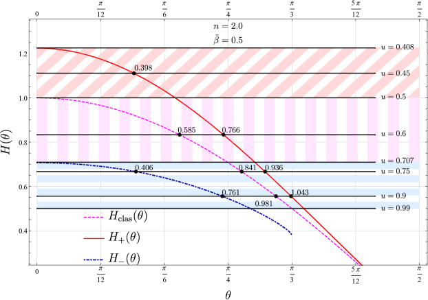
Figure 4: Plot of the functions $H_{+}(\theta)$ (solid line, red), $H_{\rm clas}(\theta)$ (dashed line, magenta) and $H_{-}(\theta)$ dash-dotted line, blue), for ${\tilde{\beta}}=0.5,\,n=2$. The horizontal lines labeled by $u=v/c$ correspond to $H=1/(nu)$ in the ordinate. The Cherenkov angles are in radians. Region A: upper white area, Region B: oblique hatched area (orange) , Region C: vertical hatched area (light magenta) and Region D: horizontal hatched area (light blue.)

In the following we list some important properties of the functions $H_{\eta}(\theta)$. They are decreasing functions of $\theta$ that satisfy $H_{-}<H_{\rm clas}<H_{+}$, for all values of $\theta$. This justifies the name of outer (inner) cone that we give to the radiation emitted at the angles $\theta_{+}$ ($\theta_{-}$), respectively.

The function $H_{+}$ is real for any value of ${\tilde{\beta}}$, while $H_{-}$ has the following restrictions: (i) it is imaginary when ${\tilde{\beta}}>1$, so that it does not contribute to the radiation in this case; (ii) when ${\tilde{\beta}}<1$, it is real only in the interval $0<\theta<\arccos{\tilde{\beta}}$, which constrains its contribution. The maximum values of each function at the origin are

$$H_{+}(\theta=0)=\sqrt{1+{\tilde{\beta}}},\quad H_{\rm clas}(\theta=0)=1,\quad H_{-}(\theta=0)=\sqrt{1-{\tilde{\beta}}}.$$ (90)

For a given material (fixed $n>1$), the evolution of the Cherenkov angles $\theta_{+},\theta_{-},\theta_{\rm clas},$ as a function of the particle velocity, $u=v/c$, are described as follows (the classical case is incorporated for comparison):

• Region A: No Cherenkov radiation when

  $$\sqrt{1+{\tilde{\beta}}}<1/(nu),$$ (91)

  corresponding to the upper white area above the $u=0.408$ horizontal line in Fig. 4.

• Region B: The region in which only $\theta_{+}$ arises is in the interval

  $$1<1/(nu)<\sqrt{1+{\tilde{\beta}}},$$ (92)

  defined by the orange oblique hatched area in Fig. 4. This is the vacuum Cherenkov radiation in the LIV case $(b\neq 0,n=1)$, which is not allowed in the classical situation POTTING1 ; POTTING2 .

• Region C: The region in which both $\theta_{+}$ and $\theta_{\rm clas}$ are present is in the interval

  $$\sqrt{1-{\tilde{\beta}}}<1/(nu)<1,$$ (93)

  shown by the pale magenta vertical hatched area in Fig. 4.

• Region D: The area in which all three angles, $\theta_{+}$, $\theta_{\rm clas}$ and $\theta_{-}$ coexist is in the interval

  $${\tilde{\beta}}\left(1-{\tilde{\beta}}^{2}\right)<1/(nu)<\sqrt{1-{\tilde{\beta}}},$$ (94)

  marked as the pale blue horizontal hatched area in Fig. 4.

• Region E: The lower region in which only $\theta_{+}$ and $\theta_{\rm clas}$ arise corresponds to the interval

  $$1/n<1/(nu)<{\tilde{\beta}}\left(1-{\tilde{\beta}}^{2}\right).$$ (95)

• The lower limit for $H=1/(nu)$ is $H=1/n$ and is given by the maximum velocity $u=1$.

The case of vacuum Cherenkov radiation ($n=1$) is illustrated in the Fig. 3 for $\beta=0.5$. A generic case for $n=2$ and ${\tilde{\beta}}=0.5$ is shown in the Fig. 4. Regions A, B, C and D are indicated in the figure caption. In this case the lower limit for $H$ is $1/2$, as approximately indicated by the horizontal line labeled by $u=0.99$. The values of the Cherenkov angles for different velocities corresponding to this case are also shown in Table 1. From the left panel of Fig. 2, we appreciate that the Cherenkov angles obtained in this case, with our choice for the SPA in Eq. (37), fall in a region where the classical SPA approximates very well the exact numerical values shown in the figure.

$u$	$\theta_{+}(\rm rad)$	$\theta_{\rm clas}(\rm rad)$	$\theta_{-}(\rm rad)$
$0.45$	$0.398$	$0.0$	$0.0$
$0.60$	$0.766$	$0.585$	$0.0$
$0.75$	$0.936$	$0.841$	$0.406$
$0.90$	$1.043$	$0.981$	$0.761$

Table 1: The possible Cherenkov angles for ${\tilde{\beta}}=0.5$ and $n=2$, exhibited in Fig. 4.

VI.4 Cherenkov angles $\theta_{+}$, $\theta_{-}$ as a function on $\beta$

In this subsection we investigate the dependence of the Cherenkov angles upon the chiral parameter $\beta=bc/\omega$, as a function of $n$ and $u$, paying attention to the points where these angles are cut down, as shown in the Fig. 5. In other words, we are interested in the functions $\theta_{\pm}(\beta)$ for fixed $n$ and $u$. Let us recall that $\beta(n)=\beta/n^{2}$. It can be shown that $\theta_{+}(\beta)$ ($\theta_{-}(\beta)$) is an increasing (decreasing) function of $\beta$.

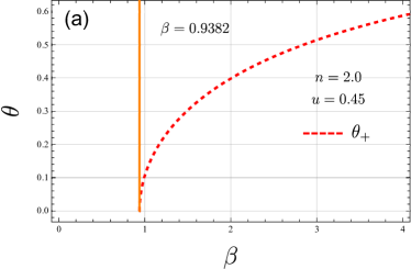
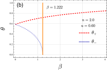
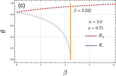
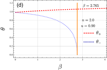
Figure 5: The Cherenkov angles $\theta_{+},\,\theta_{-}$, for $n=2$ and different values of $u$, as a function of $\beta$. Panel (a): $\theta_{+}$ vanishes at $\beta=\beta^{C}=0.938$. Panel (b): $\theta_{-}$ vanishes at $\beta=\beta^{C}=1.222$. Panel (c) : $\theta_{-}$ vanishes at $\beta=\beta^{C}=2.222$. Panel (d): $\theta_{-}$ vanishes at $\beta=\beta^{C}=2.765$.

We distinguish two cases:

1. $nu<1$. From Eqs. (92) and (93) we have only $\theta_{+}$. The angle $\theta_{+}$ starts at $\beta^{\text{C}}$, where $\theta_{+}(\beta^{\text{C}})=0$. By substituting this in Eq. (89), we obtain

   $$\beta^{\text{C}}=\frac{1}{u^{2}}-n^{2},$$ (96)

   as we can see from Fig. 5 (a).

2. $nu>1$. In this case we can have both $\theta_{+}$ and $\theta_{-}$, which start at $\beta=0$. Since $\theta_{-}$ is a decreasing function of $\beta$, we determine a cutoff $\beta^{\text{C}}$ by setting $\theta_{-}(\beta^{\text{C}})=0$. Replacing $\theta_{-}(\beta^{\text{C}})=0$ in Eq. (89) yields

   $$\beta^{\text{C}}=n^{2}-\frac{1}{u^{2}},$$ (97)

   which can be verified in Figs. 5(b-d).

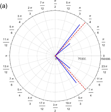
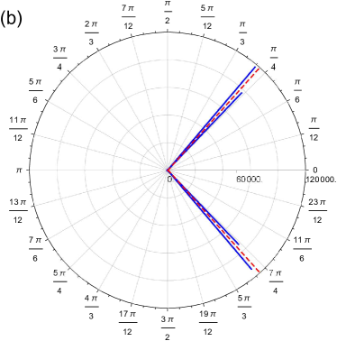
Figure 6: The angular distribution for the radiated energy per unit frequency (solid blue line) in a chiral dielectric medium with $n=2$, $\omega/c=14\;\text{$\mu$m}^{-1}$, $u=0.75$ and $\xi=100\;\text{$\mu$m}$. Panel (a) : ${\tilde{\beta}}=0.3$, and Panel (b) : ${\tilde{\beta}}=0.1$. The dashed red line corresponds to the conventional Cherenkov cone. The charge moves from left to right.

To close this section we present the figures 6(a-b) showing the SED for $n=2$, and the choices $\beta=1.2$ and $\beta=0.4$, which yield ${\tilde{\beta}}=0.3$ and ${\tilde{\beta}}=0.1$, respectively. In both figures the solid blue line corresponds to $\xi=100\;\text{$\mu$m}$ with $u=0.75$ and $\omega/c=14\;\text{$\mu$m}^{-1}$. We notice that as long as $\beta$ takes lesser values, the splitting between $\theta_{+}$ and $\theta_{-}$ closes up and the difference in the amplitudes of the lobes decreases. In Fig. 6a the angles of the chiral Cherenkov cones are $\theta_{+}=0.908$ and $\theta_{-}=0.700$, and in Fig. 6b they are $\theta_{+}=0.868$ and $\theta_{-}=0.807$. All plotted SED are expressed in units of the common factor $q^{2}/(4\pi^{2}c^{3})$ .

VII Total radiated energy per unit frequency

In this section, we calculate the total energy per unit frequency radiated by the charge on its path from $-\xi$ to $+\xi$. Also we consider the ratio of the radiated energy per unit frequency between the $\theta_{+}$ and the $\theta_{-}$ cones, as well as between them and the case of non-chiral materials $\theta_{\rm clas}$. We recall the calculation in the conventional Cherenkov case (non-chiral material), where we have

$$\begin{split}\frac{d^{2}E_{\rm{clas}}}{d\Omega d\omega}&=\frac{n\omega^{2}q^{2}}{\pi^{2}c^{3}}\left(1-\frac{c^{2}}{n^{2}v^{2}}\right)\frac{\sin^{2}[\xi\,\tilde{\Xi}]}{\tilde{\Xi}^{2}},\quad\tilde{\Xi}(\theta)=\frac{\omega}{v}\left(1-\frac{nv}{c}\cos\theta\right),\end{split}$$ (98)

given by the limit $\alpha=0$ in Eq.(88) . Axial symmetry, which is also present in our chiral case, yields

$$\frac{dE_{\rm{conv}}}{d\omega}=\frac{2n\omega^{2}q^{2}}{\pi c^{3}}\left(1-\frac{c^{2}}{n^{2}v^{2}}\right)\int_{0}^{\pi}d\theta\sin\theta\frac{\sin^{2}[\xi\,\tilde{\Xi}]}{\tilde{\Xi}^{2}}.$$ (99)

The trick to perform the remaining angular integration in the limit $\xi\rightarrow\infty$ is to use Eq. (75), obtaining

$$\frac{\sin^{2}[\xi\,\tilde{\Xi}]}{\tilde{\Xi}^{2}}=\pi\delta(\tilde{\Xi})\frac{\sin[\xi\,\tilde{\Xi}]}{\tilde{\Xi}}=\pi\xi\delta(\tilde{\Xi}),$$ (100)

leaving a final integration over $\delta(\tilde{\Xi})$. The result is

$$\frac{dE_{\rm{conv}}}{d\omega}=\frac{q^{2}\omega L}{c^{2}}\left(1-\frac{c^{2}}{n^{2}v^{2}}\right),$$ (101)

where we have denoted by $L=2\xi$ the total distance traveled by the charged particle in the medium. Let us emphasize that in general $n=n(\omega)$, which we do not consider here. From Eq. (88) we have

$$\frac{d^{2}E}{d\Omega d\omega}=\sum_{\eta=\pm 1}\frac{d^{2}E_{\eta}}{d\Omega d\omega},\qquad\frac{d^{2}E_{\eta}}{d\Omega d\omega}=\frac{n\omega^{2}q^{2}}{4\pi^{2}c^{3}}{\cal\tilde{K}}_{\eta}(\omega,\theta)\frac{\sin^{2}[\xi\tilde{\Xi}_{\eta}]}{\tilde{\Xi}^{2}_{\eta}},\qquad{\cal\tilde{K}}_{\eta}(\omega,\theta)=\frac{\mathcal{\tilde{T}}_{1,\eta}(\omega,\theta)}{\tilde{g}^{2}_{\eta}(\theta)},$$ (102)

in the chiral case. The angular integration is similar to the non-chiral case: the functions ${\cal\tilde{K}}_{\eta}(\omega,\theta)$ are evaluated at the respective Cherenkov angles $\theta_{\eta}$, while the integration over $\delta(\tilde{\Xi}_{\eta})$ is a bit more involved. The result is

$$\frac{dE_{\eta}}{d\omega}=\frac{\omega q^{2}L}{4c^{2}}\left[\frac{\sin\theta\,\cal{\tilde{K}}_{\eta}(\omega,\theta)}{\Big{|}{\sin\theta\,\tilde{C}_{\eta}(\theta)-\cos\theta\,\frac{\partial\tilde{C}_{\eta}(\theta)}{\partial\theta}}\Big{|}}\right]_{\theta=\theta_{\eta}}.$$ (103)

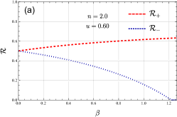
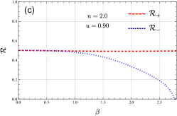
Figure 7: Ratio between the total energy per unit frequency, as a function of $\beta$, radiated by each cone ($\theta_{+},\theta_{-}$ ) in the chiral Cherenkov case, with respect to the conventional case, for $n=2.0$. Panel (a): $u=0.6$, panel (b) : $u=0.75$ and panel (c) : $u=0.9$. The dashed (red) line corresponds to ${\cal R}_{+}$ and the dotted (blue) line is for ${\cal R}_{-}$.

Now, we compare the contribution to the total energy radiated per unit frequency from each distribution in Eq. (103), as a function of the chiral parameter $\beta$. We define the ratios

$$\mathcal{R}_{\eta}=\frac{dE_{\eta}/d\omega}{dE_{\text{class}}/d\omega}=\frac{1}{4}\frac{1}{1-\frac{c^{2}}{v^{2}n^{2}}}\left[\frac{\sin\theta\,\cal{\tilde{K}}_{\eta}(\omega,\theta)}{\Big{|}{\sin\theta\,\tilde{C}_{\eta}(\theta)-\cos\theta\,\frac{\partial\tilde{C}_{\eta}(\theta)}{\partial\theta}}\Big{|}}\right]_{\theta=\theta_{\eta}},$$ (104)

which account for the fraction of the radiated energy per unit frequency that is produced by each cone in the chiral case, with respect to the energy per unit frequency emitted in the conventional case.

Figures 7(a-c) show that when $\alpha_{0}$ is close to zero the contribution of the radiation for each $\eta$ in Eq. (103) is approximately $0.5$. As $\beta$ takes larger values we see that the contribution of the radiation produced by the inner cone, $\theta_{-}$, gets smaller and smaller until it disappears completely. The value of $\beta$ at which this occurs is given by the vanishing of $\theta_{-}$ in Figs. 5 (b-d). In the limit when $\mathcal{R}_{-}$ vanishes, we observe that the contribution of the radiation from the outer cone is just a fraction of the radiation in the conventional case.

To complete the analysis, we consider the ratio

$$\mathcal{R}_{-}/\mathcal{R}_{+}=\frac{dE_{-}/d\omega}{dE_{+}/d\omega}=\frac{\sin\theta_{-}\,\cal{\tilde{K}}_{-}(\omega,\theta_{-})}{\sin\theta_{+}\,\cal{\tilde{K}}_{+}(\omega,\theta_{+})}\frac{\Big{|}{\sin\theta\,\tilde{C}_{+}-\cos\theta\,\frac{\partial\tilde{C}_{+}}{\partial\theta}}\Big{|}_{\theta=\theta_{+}}}{\Big{|}{\sin\theta\,\tilde{C}_{-}-\cos\theta\,\frac{\partial\tilde{C}_{-}}{\partial\theta}}\Big{|}_{\theta=\theta_{-}}},$$ (105)

which is a measure of how larger the contribution to the radiation from the inner cone is with respect to the outer one. Figures 8(a-c) show that the output from the inner cone is always smaller than that from the outer cone. This ratio decreases as $\beta$ takes larger values, until it gets to zero when the inner cone vanishes.

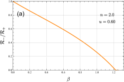
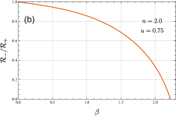
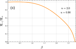
Figure 8: Ratio between the total energy radiated by the inner Cherenkov cone with respect to the outer one, for $n=2.0$. Panel (a) : $u=0.6$, panel (b) : $u=0,75$ and panel (c) : $u=0.9$.

VIII Summary and conclusions

In the far field approximation, we study the electromagnetic response of a non magnetic chiral media to arbitrary time-dependent sources in the framework of the Carroll, Field and Jackiw (CFJ) electrodynamics, which includes the additional parameters $b_{0}$ and $\mathbf{b}$ giving rise to the magnetoelectric effect. Examples of materials described by this effective electrodynamics are the Weyl semimetals, where these parameters describe the separation of the Weyl points in energy ($b_{0}$) and momentum ($\mathbf{b}$), in the reciprocal space. It is interesting to remark that this model also arises in the CPT-odd sector of the Standard Model Extension designed to probe Lorentz invariance violations in fundamental interactions. We restrict ourselves to the case $b_{0}=0$ and choose the $z$ axis of our coordinate system in the direction of $\mathbf{b}$. Most of our calculations are performed in vacuum ($n=1$) and the generalization to arbitrary ponderable media required to deal with a real material is performed following the substitutions indicated in the Appendix B.

As discussed in section II, the linear dependence $\theta(x)=b_{\mu}x^{\mu}$ on the coordinates in the CFJ electrodynamics preserves the invariance under translations of the Lagrangian density up to a total derivative. The system has axial symmetry with respect to the vector $\mathbf{b}$. In Eq. (20) we obtained the Green’s function (GF) of the system, $G^{\mu\nu}(x,x^{\prime})$, in terms of a differential matrix operator acting on the scalar function $f(\mathbf{x},\mathbf{x^{\prime}},\omega)$, given in Eq. (28). This function exhibits two contributions accounting for the birefringence of the medium, which are inherited by the remaining observables. The next step was to calculate the general expression for the GF in the radiation zone. To this end we considered the stationary phase approximation in the far zone ($R\rightarrow\infty$), where the function $f(\mathbf{x},\mathbf{x^{\prime}},\omega)$ is highly oscillating according to $\exp(iR\,h_{\eta}(k_{\perp}))$ in Eqs. (31) and (33). Still, the resulting stationary phase equation (34) is quartic in the momentum, which called for a further approximation to keep an analytic calculation. We studied the numerical solution of Eq. (34) and concluded that, within specific ranges of the observation angle $\theta$, the choice in Eq. (37), corresponding to the conventional case with $\mathbf{b}=0$, is adequate. A qualitative measure of how good this approximation is for increasing values of $\beta=c|\mathbf{b}|/\omega$ is shown in Fig. 2. Yet at the end of the calculation of a Cherenkov angle one should identify its position in the corresponding graph in order to asses it validity. Next, for an arbitrary source we determine the electromagnetic potentials in the radiation zone and give a general expression for the electromagnetic fields in Eqs. (59) and (60). We show that the triad ${\mbox{\boldmath$\hat{n}$}},\mathbf{E},\mathbf{B}$ is not orthogonal and explain how the conventional case is obtained. The general expression for the spectral distribution of the radiation follows from the Eqs. (54), (147), (153) and (154). Some symmetry properties of the fields under the change $\omega\rightarrow-\omega$ are useful to show that this rather complicated expression is real, as expected. Also at each step in the calculation we able to recover the well known conventional results by setting $b=0$.

Next we turn to the particular case of Cherenkov radiation where the source is a charge moving at constant velocity parallel to $\mathbf{b}$, thus ignoring recoil effects. The electromagnetic potentials and fields results by the direct substitution of the charge current in the previous general expressions. In analogy with the conventional case, substantial simplifications arise from the form of the outgoing radiation wave which now acquires additional angular dependence which modify the conventional Cherenkov condition. Yet this condition also arises as a delta-like contribution in the spectral distribution of the radiation which fixes the allowed angles according to the Eq. (76), which is conveniently written as $H_{\eta}(\theta)=c/nv$ as in Eq. (89). Then, for given values of $b,n$ and $u=v/c$, the Cherenkov angles are determined by the intersection of $H_{\eta}$ with the straight line $1/nu$, as shown in Figs 3 and 4, where we also plot the conventional case $H_{{\rm clas}}(\theta)$ for comparison. The functions $H(\theta)$ are decreasing in the angle. Figure 3 is for $n=1$ and depicts what is normally called vacuum Cherenkov radiation that is forbidden in the conventional case. Here only the angle $\theta_{+}$ is present. Figure 4 is for $n>1$ and shows zero, one or two Cherenkov angles. The limits of such regions is determined by the maximum values $H(\theta=0)$ in the following way: (i) no Cherenkov angle occurs when $1/nu>H_{+}(0)$, (ii) when $1/nu<H_{+}(0)$ the angle $\theta_{+}$ is always present and starts to be accompanied by the conventional angle when $1/nu<1$. The angle $\theta_{-}$ occurs only in the interval $\alpha(n)(1-\alpha^{2}(n)<1/nu<H_{-}(0)$. To avoid confusion, let us observe that the horizontal lines labeled by $u$ in those figures correspond to the value $1/nu$ in the ordinate. The relation $\theta_{-}<\theta_{\rm clas}<\theta_{+}$ always hold and $\theta_{\pm}$ merge into $\theta_{\rm clas}$ as $|\mathbf{b}|\rightarrow 0$.

We also study the dependence of the angles $\theta_{\pm}$ as a function of the chiral parameter $\beta$ for fixed $n$ and $u$. As shown in Fig. 5, we find two relevant cases: (1) for $nu<1$ we only have $\theta_{+}$ which starts at the minimum $\beta$ determined by the Eq. (96), (2) for $nu>1$ both $\theta_{\pm}$ start at $\beta=0$. While $\theta_{+}$ is an increasing function, $\theta_{-}$ is a decreasing one which reaches zero at a value given by the Eq. (97).

Angular plots of the spectral distribution are presented in the Fig. 6, showing the separation of the cones as ${\tilde{\beta}}$ increases. Also a qualitative measure of the energy output of each cone in given by the length of the radial lines, showing that $\theta_{-}$ radiates less than $\theta_{+}$. A better comparison is obtained by calculating the ratios of the energy per unit frequency radiated in the $\theta_{\pm}$ cones with respect to the conventional case (Fig. 7). We find that the contribution of the outer cone ($\theta_{+}$) gets bigger, while that of the inner cone ($\theta_{-}$) gets smaller as $\beta=cb/\omega$ takes larger values, until it reaches the value zero. This behavior is also evident in Fig. 8, which depicts the ratio of the energy radiated per unit frequency between the $\theta_{-}$ and the $\theta_{+}$ cones.

We successfully compare our result for the vacuum Cherenkov angle $\theta_{+}$ with that obtained in Eq. (40) of Ref. TUCHIN3 in the high energy approximation. This requires $\theta_{+}<<1$, $\beta=bc/\omega<<1$, together with a highly relativistic velocity for the charge, which we take as $v=c$. Under these conditions, our Eq. (76) reduces to

$$\cos\theta_{+}\left[1+\frac{1}{2}\beta\cos\theta_{+}\right]=1,$$ (106)

whose solution yields $\cos\theta_{+}=1-{\beta}/{2}$, providing $\theta_{+}=\sqrt{\beta}$ in the small angle approximation. This result is precisely that of Ref. TUCHIN3 , restricted to our case when $\mathbf{v}$ is parallel to $\mathbf{b}$ and $\lambda=+$.

We expect that our general description of radiation in chiral matter provides the basis for the study of further processes such as Cherenkov radiation with a charge velocity $\mathbf{v}$ in arbitrary direction with respect to $\mathbf{b}$, charged particle energy losses and synchrotron radiation, for example. Regarding the case of Cherenkov radiation and without entering in any experimental detail, which is far beyond our theoretical understanding, we envisage that the two Cherenkov angles predicted in this work could be measured by sending the charge through a slab of material and using either a differential Cherenkov counter or a ring imaging Cherenkov counter ratcliff . It is interesting to observe that the measure of $\theta_{+}$ would provide an optical experimental determination of the parameter $|\mathbf{b}|$ of the chiral medium, according to the expression

$$|\mathbf{b}|=n^{2}\left(\frac{\omega}{c}\right)\frac{1}{\cos^{5}\theta_{+}}\left(\frac{c}{nv}-\cos\theta_{+}+2\cos^{3}\theta_{+}\right)\left(\frac{c}{nv}-\cos\theta_{+}\right).$$ (107)

When both $\theta_{\pm}$ are present, $|\mathbf{b}|$ can be determined from the measurement of either one, and consistency yields a relationship between $\theta_{+}$ and $\theta_{-}$, which is not very illuminating to be presented explicitly. In our restricted formulation ($\mathbf{v}$ parallel to $\mathbf{b}$) at least one should know the direction of $\mathbf{b}$ in the sample to correctly send the incident charge parallel to $\mathbf{b}$. Due to the far reaching applications of Cherenkov radiation and since chiral matter constitutes a genuine new state of matter recently discovered, it could prove valuable to study its practical applications as a Cherenkov radiator.

Appendix A The calculation of the GF in the radiation zone

In this Appendix we summarize the calculation of the GF (20) in the far-field approximation, using the stationary phase method. We start from the splitting of the GF introduced in Eqs. (42), (43) and (44).

A.1 $G^{\mu\nu}_{0}(\mathbf{x},\mathbf{x^{\prime}};\omega)$ in the far-field approximation

Using $k^{2}=k_{0}^{2}-k_{\perp}^{2}+\partial_{Z}^{2}$ we further split $G^{\mu\nu}_{0}(\mathbf{x},\mathbf{x^{\prime}};\omega)$ into

$$\begin{split}G^{\mu\nu}_{0}(\mathbf{x},\mathbf{x^{\prime}};\omega)&=-\eta^{\mu\nu}k_{0}^{2}\frac{i}{16\pi b}\int^{\infty}_{-\infty}\frac{dk_{\perp}k_{\perp}}{k_{\parallel}}H_{0}^{(1)}(k_{\perp}R_{\perp})\left[\frac{e^{i\sqrt{k_{\parallel}^{2}+bk_{\parallel}}Z}}{\sqrt{k_{\parallel}^{2}+bk_{\parallel}}}-\frac{e^{i\sqrt{k_{\parallel}^{2}-bk_{\parallel}}Z}}{\sqrt{k_{\parallel}^{2}-bk_{\parallel}}}\right]\\ &+\eta^{\mu\nu}\frac{i}{16\pi b}\int^{\infty}_{-\infty}\frac{dk_{\perp}k_{\perp}k^{2}_{\perp}}{k_{\parallel}}H_{0}^{(1)}(k_{\perp}R_{\perp})\left[\frac{e^{i\sqrt{k_{\parallel}^{2}+bk_{\parallel}}Z}}{\sqrt{k_{\parallel}^{2}+bk_{\parallel}}}-\frac{e^{i\sqrt{k_{\parallel}^{2}-bk_{\parallel}}Z}}{\sqrt{k_{\parallel}^{2}-bk_{\parallel}}}\right]\\ &-\eta^{\mu\nu}\partial^{2}_{Z}\frac{i}{16\pi b}\int^{\infty}_{-\infty}\frac{dk_{\perp}k_{\perp}}{k_{\parallel}}H_{0}^{(1)}(k_{\perp}R_{\perp})\left[\frac{e^{i\sqrt{k_{\parallel}^{2}+bk_{\parallel}}Z}}{\sqrt{k_{\parallel}^{2}+bk_{\parallel}}}-\frac{e^{i\sqrt{k_{\parallel}^{2}-bk_{\parallel}}Z}}{\sqrt{k_{\parallel}^{2}-bk_{\parallel}}}\right].\end{split}$$ (108)

These three terms can be integrated using the stationary phase method in the same way as we have computed the function

$$f(\mathbf{x},\mathbf{x^{\prime}};\omega)=\frac{i}{16\pi b}\int^{\infty}_{-\infty}\frac{dk_{\perp}k_{\perp}}{k_{\parallel}}H_{0}^{(1)}(k_{\perp}R_{\perp})\left[\frac{e^{i\sqrt{k_{\parallel}^{2}+bk_{\parallel}}Z}}{\sqrt{k_{\parallel}^{2}+bk_{\parallel}}}-\frac{e^{i\sqrt{k_{\parallel}^{2}-bk_{\parallel}}Z}}{\sqrt{k_{\parallel}^{2}-bk_{\parallel}}}\right],$$ (109)

in the far-field approximation, previously obtaining

$$\mathfrak{f}(\mathbf{x},\mathbf{x^{\prime}};\omega)=\frac{1}{8\pi r}\frac{1}{k_{0}b\cos\theta}\left[\frac{e^{ik_{0}C_{+}(\theta)(r-\hat{n}\cdot\mathbf{x^{\prime}})}}{g_{+}(\theta)}-\frac{e^{ik_{0}C_{-}(\theta)(r-\hat{n}\cdot\mathbf{x^{\prime}})}}{g_{-}(\theta)}\right],$$ (110)

in Eq. (38), with $k_{0}=\omega/c$. Let us recall that we are denoting by $\mathfrak{f}(\mathbf{x},\mathbf{x^{\prime}};\omega)$ the function ${f}(\mathbf{x},\mathbf{x^{\prime}};\omega)$ evaluated in SPA and that according to our additional approximation in the SPA we set

$$(k_{\parallel})_{s}=k_{0}\cos\theta,\qquad(k_{\perp})_{s}=k_{0}\sin\theta,$$ (111)

in the final result.

The first integral in (108) is proportional to $f$ yielding the contribution

$$-\eta^{\mu\nu}k^{2}_{0}\,\mathfrak{f}(\mathbf{x},\mathbf{x^{\prime}};\omega),$$ (112)

in the SPA. The second one has an extra factor of $k_{\perp}^{2}$ in the integrand, which is evaluated in the stationary phase point (111), giving the contribution

$$\eta^{\mu\nu}k_{0}^{2}\sin^{2}\theta\,\mathfrak{f}(\mathbf{x},\mathbf{x^{\prime}};\omega).$$ (113)

The third term in (108) requires the second derivative with respect Z, which is

$$\partial^{2}_{Z}\left[\frac{e^{i\sqrt{k_{\parallel}^{2}+bk_{\parallel}}Z}}{\sqrt{k_{\parallel}^{2}+bk_{\parallel}}}-\frac{e^{i\sqrt{k_{\parallel}^{2}-bk_{\parallel}}Z}}{\sqrt{k_{\parallel}^{2}-bk_{\parallel}}}\right]=-\left[\sqrt{k_{\parallel}^{2}+bk_{\parallel}}e^{i\sqrt{k_{\parallel}^{2}+bk_{\parallel}}Z}-\sqrt{k_{\parallel}^{2}-bk_{\parallel}}e^{i\sqrt{k_{\parallel}^{2}-bk_{\parallel}}Z}\right],$$ (114)

and can be rewritten as

$$\begin{split}\eta^{\mu\nu}\frac{i}{16\pi b}&\int^{\infty}_{-\infty}\frac{dk_{\perp}k_{\perp}}{k_{\parallel}}H_{0}^{(1)}(k_{\perp}R_{\perp})\left[(k_{\parallel}^{2}+bk_{\parallel})\frac{e^{i\sqrt{k_{\parallel}^{2}+bk_{\parallel}}Z}}{\sqrt{k_{\parallel}^{2}+bk_{\parallel}}}-(k_{\parallel}^{2}-bk_{\parallel})\frac{e^{i\sqrt{k_{\parallel}^{2}-bk_{\parallel}}Z}}{\sqrt{k_{\parallel}^{2}-bk_{\parallel}}}\right],\\ &=\eta^{\mu\nu}k_{0}^{2}\cos^{2}\theta\Big{[}(1+\alpha\sec\theta)\mathfrak{f}_{+}(\mathbf{x},\mathbf{x^{\prime}};\omega)-(1-\alpha\sec\theta)\mathfrak{f}_{-}(\mathbf{x},\mathbf{x^{\prime}};\omega)\Big{]},\end{split}$$ (115)

after evaluating the additional factors in the SPA. Substituting (113) and (115) into (108), we finally obtain

$$G^{\mu\nu}_{0}(\mathbf{x},\mathbf{x^{\prime}};\omega)=\eta^{\mu\nu}\frac{1}{8\pi r}\left[\frac{e^{ik_{0}C_{+}(\theta)(r-\hat{n}\cdot\mathbf{x^{\prime}})}}{g_{+}(\theta)}+\frac{e^{ik_{0}C_{-}(\theta)(r-\hat{n}\cdot\mathbf{x^{\prime}})}}{g_{-}(\theta)}\right].$$ (116)

A.2 $G^{\mu\nu}_{\text{\tiny{b}}}(\mathbf{x},\mathbf{x^{\prime}};\omega)$ in the far-field approximation

Our starting point is the contribution linear in $b$ in the second Eq.(20), which we rewrite

$$G^{\;\;\mu\nu}_{\text{\tiny{b}}\;\;}(\mathbf{x},\mathbf{x^{\prime}};\omega)=ib\epsilon^{\mu\nu\sigma 3}\int\frac{d^{3}\mathbf{k}}{(2\pi)^{3}}\frac{k_{\sigma}}{k^{4}+\tilde{b}^{2}k^{2}-(\tilde{b}\cdot k)^{2}}e^{i\mathbf{k}\cdot(\mathbf{x}-\mathbf{x^{\prime}})}.$$ (117)

Here $\sigma=0,1,2$ and $k_{\sigma}=(k_{0},-\mathbf{k})$. It is convenient to define the following integral

$$I_{\alpha}(\mathbf{x},\mathbf{x^{\prime}};\omega)=\int\frac{d^{3}\mathbf{k}}{(2\pi)^{3}}\frac{k_{\alpha}}{k^{4}+\tilde{b}^{2}k^{2}-(\tilde{b}\cdot k)^{2}}e^{i\mathbf{k}\cdot(\mathbf{x}-\mathbf{x^{\prime}})},$$ (118)

such that

$$G_{b}^{\mu\nu}=ib\epsilon^{\mu\nu\sigma 3}I_{\sigma}.$$ (119)

For $\sigma=0$ we have straightforward result

$$I_{0}(\mathbf{x},\mathbf{x^{\prime}};\omega)=k_{0}\,\mathfrak{f}(\mathbf{x},\mathbf{x^{\prime}};\omega).$$ (120)

Also, the contribution from $I_{3}(\mathbf{x},\mathbf{x^{\prime}};\omega)$ yields zero in the GF due to the Levi-Civita tensor.

Next we consider $\sigma=i=1,2$, and we perform the integration of $k_{z}$ in the complex plane, as we did previously in the calculation yielding Eq. (28). We are left with

$$I^{i}(\mathbf{x},\mathbf{x^{\prime}};\omega)=\ \frac{1}{(2\pi)^{3}}\int^{\infty}_{0}dk_{\perp}k_{\perp}\int^{2\pi}_{0}d\phi\,k^{i}e^{ik_{\perp}R_{\perp}\cos\phi}\int^{\infty}_{-\infty}dk_{z}\frac{e^{ik_{z}Z}}{(k_{0}^{2}-\mathbf{k}^{2})^{2}-b^{2}(k_{0}^{2}-\mathbf{k}^{2})-b^{2}k_{z}^{2}},$$

$$\hskip 62.59596pt=\frac{i}{16\pi^{2}b}\int^{\infty}_{0}\frac{dk_{\perp}k^{2}_{\perp}}{k_{\parallel}}\int^{2\pi}_{0}d\phi\begin{bmatrix}\cos\phi\\ \sin\phi\end{bmatrix}e^{ik_{\perp}R_{\perp}\cos\phi}\left[\frac{e^{i\sqrt{k_{\parallel}^{2}+bk_{\parallel}}Z}}{\sqrt{k_{\parallel}^{2}+bk_{\parallel}}}-\frac{e^{i\sqrt{k_{\parallel}^{2}-bk_{\parallel}}Z}}{\sqrt{k_{\parallel}^{2}-bk_{\parallel}}}\right],$$

(121)

where we recall that $\phi$ is the angle between ${\mathbf{R}}_{\perp}$ and ${\mathbf{k}}_{\perp}$. In the second line of (121) we have chosen a coordinate system $\cal{S}$ with the $x$-axis in the direction of ${\mathbf{R}}_{\perp}$, such that $k^{1}=k_{\perp}\cos\phi$ and $k^{2}=k_{\perp}\sin\phi$. The angular integrals are

$$\int^{2\pi}_{0}d\phi\cos\phi e^{ik_{\perp}R_{\perp}\cos\phi}=2\pi iJ_{1}(k_{\perp}R_{\perp}),\qquad\int^{2\pi}_{0}d\phi\sin\phi e^{ik_{\perp}R_{\perp}\cos\phi}=0.$$ (122)

Using the recurrence

$$J_{1}(k_{\perp}R_{\perp})=-\frac{1}{k_{\perp}}\frac{\partial}{\partial R_{\perp}}J_{0}(k_{\perp}R_{\perp}),$$ (123)

the integral (121) can be written as

$$\begin{split}\mathbf{I}_{\mathcal{S}}(\mathbf{x},\mathbf{x^{\prime}};\omega)&=-\frac{1}{8\pi^{2}b}\int^{\infty}_{0}\frac{dk_{\perp}k^{2}_{\perp}}{k_{\parallel}}\begin{bmatrix}J_{1}(k_{\perp}R_{\perp})\\ 0\end{bmatrix}\left[\frac{e^{i\sqrt{k_{\parallel}^{2}+bk_{\parallel}}Z}}{\sqrt{k_{\parallel}^{2}+bk_{\parallel}}}-\frac{e^{i\sqrt{k_{\parallel}^{2}-bk_{\parallel}}Z}}{\sqrt{k_{\parallel}^{2}-bk_{\parallel}}}\right],\\ &=\frac{\partial}{\partial R_{\perp}}\frac{1}{16\pi b}\int^{\infty}_{-\infty}\frac{dk_{\perp}k_{\perp}}{k_{\parallel}}\begin{bmatrix}H_{0}(k_{\perp}R_{\perp})\\ 0\end{bmatrix}\left[\frac{e^{i\sqrt{k_{\parallel}^{2}+bk_{\parallel}}Z}}{\sqrt{k_{\parallel}^{2}+bk_{\parallel}}}-\frac{e^{i\sqrt{k_{\parallel}^{2}-bk_{\parallel}}Z}}{\sqrt{k_{\parallel}^{2}-bk_{\parallel}}}\right],\\ &=\frac{1}{i}\begin{bmatrix}1\\ 0\end{bmatrix}\frac{\partial}{\partial R_{\perp}}f(\mathbf{x},\mathbf{x^{\prime}};\omega).\end{split}$$ (124)

In the chosen coordinate system we have $I^{2}=0$. Then the vector $\mathbf{I}(\mathbf{x},\mathbf{x^{\prime}};\omega)=(I^{1},0)$ is parallel to $\mathbf{R_{\perp}}$ and we can write the general result

$$\mathbf{I}(\mathbf{x},\mathbf{x^{\prime}};\omega)=\frac{1}{i}\frac{(\mathbf{x}-\mathbf{x^{\prime}})_{\perp}}{R_{\perp}}\frac{\partial}{\partial R_{\perp}}f(\mathbf{x},\mathbf{x^{\prime}};\omega).$$ (125)

From the recurrence relations of the Hankel functions we obtain

$$\frac{\partial}{\partial R_{\perp}}H_{0}^{(1)}(k_{\perp}R_{\perp})=k_{\perp}\frac{\partial}{\partial(k_{\perp}R_{\perp})}H_{0}^{(1)}(k_{\perp}R_{\perp})=-k_{\perp}H_{1}^{(1)}(k_{\perp}R_{\perp}),$$ (126)

which yields

$$\frac{\partial}{\partial R_{\perp}}f(\mathbf{x},\mathbf{x^{\prime}};\omega)=-\frac{i}{16\pi b}\int^{\infty}_{-\infty}\frac{dk_{\perp}k^{2}_{\perp}}{k_{\parallel}}H_{1}^{(1)}(k_{\perp}R_{\perp})\left[\frac{e^{i\sqrt{k_{\parallel}^{2}+bk_{\parallel}}Z}}{\sqrt{k_{\parallel}^{2}+bk_{\parallel}}}-\frac{e^{i\sqrt{k_{\parallel}^{2}-bk_{\parallel}}Z}}{\sqrt{k_{\parallel}^{2}-bk_{\parallel}}}\right].$$ (127)

In the asymptotic limit $k_{\perp}R_{\perp}\rightarrow\infty$, we can approximate abramowitz

$$H_{1}^{(1)}(k_{\perp}R_{\perp})=\sqrt{\frac{2}{\pi k_{\perp}R_{\perp}}}e^{ik_{\perp}R_{\perp}-i\frac{\pi}{4}}e^{-i\frac{\pi}{2}}=H_{0}^{(1)}(k_{\perp}R_{\perp})e^{-i\frac{\pi}{2}}=-iH_{0}^{(1)}(k_{\perp}R_{\perp}),$$ (128)

$$\frac{\partial}{\partial R_{\perp}}f(\mathbf{x},\mathbf{x^{\prime}};\omega)=i\frac{i}{16\pi b}\int^{\infty}_{-\infty}\frac{dk_{\perp}k^{2}_{\perp}}{k_{\parallel}}\,H_{0}^{(1)}(k_{\perp}R_{\perp})\,\left[\frac{e^{i\sqrt{k_{\parallel}^{2}+bk_{\parallel}}Z}}{\sqrt{k_{\parallel}^{2}+bk_{\parallel}}}-\frac{e^{i\sqrt{k_{\parallel}^{2}-bk_{\parallel}}Z}}{\sqrt{k_{\parallel}^{2}-bk_{\parallel}}}\right],\\$$ (129)

which again has the form of the function $f(\mathbf{x},\mathbf{x^{\prime}};\omega)$ in Eq. (109), except for an additional factor $k_{\perp}$ in the integrand. In the SPA this implies

$$\frac{\partial}{\partial R_{\perp}}f(\mathbf{x},\mathbf{x^{\prime}};\omega)=ik_{0}\sin\theta\,\mathfrak{f}(\mathbf{x},\mathbf{x^{\prime}};\omega),\quad\rightarrow\quad\mathbf{I}(\mathbf{x},\mathbf{x^{\prime}};\omega)=k_{0}\hat{\mathbf{n}}_{\perp}\mathfrak{f}(\mathbf{x},\mathbf{x^{\prime}};\omega),$$ (130)

where $\hat{\mathbf{n}}_{\perp}=(\sin\theta\cos\phi,\sin\theta\sin\phi)$. This completes the calculation of $G_{b}^{\mu\nu}$ in Eq. (43).

A.3 $G^{\mu\nu}_{\text{\tiny{b}}^{2}}(\mathbf{x},\mathbf{x^{\prime}};\omega)$ in the far-field approximation

This term is the easiest to calculate, because it is proportional to $f(\mathbf{x},\mathbf{x^{\prime}};\omega)$, with

$$G^{\mu\nu}_{\text{\tiny{b}}^{2}}(\mathbf{x},\mathbf{x^{\prime}};\omega)=-\tilde{b}^{\mu}\tilde{b}^{\nu}f(\mathbf{x},\mathbf{x^{\prime}};\omega).$$ (131)

The only non-zero contribution in SPA is

$$G^{33}_{\text{\tiny{b}}^{2}}(\mathbf{x},\mathbf{x^{\prime}};\omega)=-b^{2}\mathfrak{f}(\mathbf{x},\mathbf{x^{\prime}};\omega).$$ (132)

Appendix B Electromagnetic fields and the spectral distibution of the radiation for $n=1$

First we write the Cartesian components of $A^{\mu}$ for an arbitrary current $J^{\mu}(\mathbf{x^{\prime}},\omega)$ in terms of the Fourier transform ${\cal J}^{\mu}({\mathbf{k}}_{\eta},\omega)$, defined in Eq. (52), which we denote as ${\cal J}^{\mu}_{\eta}$. From Eq. (51) and in the notation of Eq. (56) we have

$${\cal A}^{0}_{\eta}(\mathbf{\hat{n}},\omega)={\cal J}^{0}_{\eta}+i\eta\tan\theta\sin\phi\,{\cal J}^{1}_{\eta}-i\eta\tan\theta\cos\phi\,{\cal J}^{2}_{\eta},$$

$${\cal A}^{1}_{\eta}(\mathbf{\hat{n}},\omega)=i\eta\tan\theta\sin\phi\,{\cal J}^{0}_{\eta}+{\cal J}^{1}_{\eta}-i\eta\sec\theta\,{\cal J}^{2}_{\eta},$$

$${\cal A}^{2}_{\eta}(\mathbf{\hat{n}},\omega)=-i\eta\tan\theta\cos\phi\,{\cal J}^{0}_{\eta}+i\eta\sec\theta\,{\cal J}^{1}_{\eta}+{\cal J}^{2}_{\eta},$$

$${\cal A}^{3}_{\eta}(\mathbf{x},\omega)=(1+\eta\,\beta\sec\theta){\cal J}^{3}_{\eta}.$$ (133)

The transformation to spherical coordinates yields

$${\cal A}^{r}_{\eta}(\mathbf{\hat{n}},\omega) = \sin\theta\cos\phi{\cal A}^{1}_{\eta}+\sin\theta\sin\phi{\cal A}^{2}_{\eta}+\cos\theta{\cal A}^{3}_{\eta},$$

$${\cal A}^{\theta}_{\eta}(\mathbf{\hat{n}},\omega) = \cos\theta\cos\phi{\cal A}^{1}_{\eta}+\cos\theta\sin\theta{\cal A}^{2}_{\eta}-\sin\theta{\cal A}^{3}_{\eta},$$ (134)

$${\cal A}^{\phi}_{\eta}(\mathbf{\hat{n}},\omega) = -\sin\theta{\cal A}^{1}_{\eta}+\cos\phi{\cal A}^{2}_{\eta}.$$ (135)

Using Eq. (57) for the expression of the gradient operator in the radiation zone in the conventional relations

$$\mathbf{E}(\mathbf{x},\omega)=ik_{0}\mathbf{A}(\mathbf{x},\omega)-\mbox{\boldmath$\nabla$}A^{0}(\mathbf{x},\omega),\qquad\mathbf{B}(\mathbf{x},\omega)=\mbox{\boldmath$\nabla$}\times\mathbf{A}(\mathbf{x},\omega),$$ (136)

and splitting the electromagnetic fields as shown in Eqs. (59) and (60) we have

$$\mathbf{E}_{\eta}(\mathbf{x},\omega)=ik_{0}\left(\mathbf{A}_{\eta}(\mathbf{x},\omega)-{\mathbf{N}}_{\eta}A^{0}_{\eta}(\mathbf{x},\omega)\right),$$ (137)

$$\mathbf{B}_{\eta}(\mathbf{x},\omega)={\mathbf{N}}_{\eta}\times\mathbf{E}_{\eta}(\mathbf{x},\omega),$$ (138)

recalling the definition of ${\mathbf{N}}_{\eta}$ in Eq. (58). The explicit form of the radiation electric field in spherical coordinates is

$$\mathbf{E}_{\eta}(\mathbf{x},\omega)=ik_{0}\left[\left(A^{r}_{\eta}-C_{\eta}A^{0}_{\eta}\right)\hat{{\mathbf{r}}}+\left(A^{\theta}_{\eta}-\frac{\partial C_{\eta}}{\partial\theta}A^{0}_{\eta}\right)\mbox{\boldmath$\hat{\theta}$}+A^{\phi}_{\eta}\,\mbox{\boldmath$\hat{\phi}$}\right],$$ (139)

Now we are in position to calculate the spectral energy distribution (SED) of the radiation: the energy radiated per unit solid angle and per unit frequency. We have taken $b_{0}=0$ which yield the Poynting vector

$$\mathbf{S}(\mathbf{x},t)=\frac{c}{4\pi}\mathbf{E}(\mathbf{x},t)\times\mathbf{B}(\mathbf{x},t).$$ (140)

Thus, the total radiated energy crossing the area $\hat{{\mathbf{r}}}\,dA$ is

$$\begin{split}\int_{-\infty}^{\infty}dt(\hat{\mathbf{r}}\cdot\mathbf{S}(\mathbf{x},t))\,dA&=\frac{c}{4\pi}\int_{-\infty}^{\infty}\frac{d\omega}{2\pi}\,\hat{\mathbf{r}}\cdot\left(\mathbf{E}^{*}(\mathbf{x},\omega)\times\mathbf{B}(\mathbf{x},\omega)\right)\,dA,\\ &=\frac{c}{4\pi^{2}}\int_{0}^{\infty}d\omega\,\hat{\mathbf{r}}\cdot{\rm Re}\Big{[}\mathbf{E}^{*}(\mathbf{x},\omega)\times\mathbf{B}(\mathbf{x},\omega)\Big{]}r^{2}d\Omega,\end{split}$$ (141)

where $dA=r^{2}d\Omega$ and we read the SED

$$\frac{d^{2}E}{d\Omega d\omega}=\frac{c}{4\pi^{2}}r^{2}\,\hat{\mathbf{r}}\cdot{\rm Re}\Big{[}\mathbf{E}^{*}(\mathbf{x},\omega)\times\mathbf{B}(\mathbf{x},\omega)\Big{]}.$$ (142)

The last step in Eq. (141) is a consequence of the relation

$$\mathbf{E}^{*}(\mathbf{x},-\omega)\times\mathbf{B}(\mathbf{x},-\omega)=\mathbf{E}(\mathbf{x},\omega)\times\mathbf{B}^{*}(\mathbf{x},\omega)=(\mathbf{E}^{*}(\mathbf{x},\omega)\times\mathbf{B}(\mathbf{x},\omega))^{*},$$ (143)

in the integral $-\infty<\omega<+\infty$, which follows because the electromagnetic fields are real in coordinate space. Now we calculate the term

$$\mathbf{E}^{*}(\mathbf{x},\omega)\times\mathbf{B}(\mathbf{x},\omega)=\sum_{\eta,\eta^{\prime}=\pm 1}\mathbf{E}^{*}_{\eta^{\prime}}(\mathbf{x},\omega)\times\mathbf{B}_{\eta}(\mathbf{x},\omega).$$ (144)

From Eq. (138) we have

$$\mathbf{E}^{*}_{\eta^{\prime}}\times\mathbf{B}_{\eta}=\mathbf{E}^{*}_{\eta^{\prime}}(\mathbf{x},\omega)\times\left[{\mathbf{N}}_{\eta}\times\mathbf{E}_{\eta}(\mathbf{x},\omega)\right]\\ =(\mathbf{E}^{*}_{\eta^{\prime}}\cdot\mathbf{E}_{\eta}){\mathbf{N}}_{\eta}-(\mathbf{E}^{*}_{\eta^{\prime}}\cdot{\mathbf{N}}_{\eta})\mathbf{E}_{\eta}.$$ (145)

Fom Eq. (139), the electric field can be rewritten in spherical components as

$$\mathbf{E}_{\eta}(\mathbf{x},\omega)=ik_{0}\Big{[}\mathcal{E}^{r}_{\eta}\hat{{\mathbf{r}}}+\mathcal{E}^{\theta}_{\eta}\mbox{\boldmath$\hat{\theta}$}+\mathcal{E}^{\phi}_{\eta}\mbox{\boldmath$\hat{\phi}$}\Big{]},$$

$$\mathbf{E}^{*}_{\eta^{\prime}}(\mathbf{x},\omega)=-ik_{0}\Big{[}(\mathcal{E}^{r}_{\eta^{\prime}})^{*}\hat{{\mathbf{r}}}+(\mathcal{E}^{\theta}_{\eta^{\prime}})^{*}\mbox{\boldmath$\hat{\theta}$}+(\mathcal{E}^{\phi}_{\eta^{\prime}})^{*}\mbox{\boldmath$\hat{\phi}$}\Big{]},$$ (146)

where

$$\mathcal{E}_{\eta}^{r} = A^{r}_{\eta}-C_{\eta}A^{0}_{\eta},\qquad\mathcal{E}_{\eta}^{\theta}=A^{\theta}_{\eta}-\frac{\partial C_{\eta}}{\partial\theta}A^{0}_{\eta},\qquad\mathcal{E}_{\eta}^{\phi}=A^{\phi}_{\eta}.$$ (147)

With these we compute

$$\mathbf{E}^{*}_{\eta^{\prime}}\cdot{\mathbf{N}}_{\eta}=\mathbf{E}^{*}_{\eta^{\prime}}\cdot\left(C_{\eta}\mbox{\boldmath$\hat{r}$}+\frac{\partial C_{\eta}}{\partial\theta}\mbox{\boldmath$\hat{\theta}$}\right)=-ik_{0}\left[(\mathcal{E}^{r}_{\eta^{\prime}})^{*}C_{\eta}+(\mathcal{E}^{\theta}_{\eta^{\prime}})^{*}\frac{\partial C_{\eta}}{\partial\theta}\right],$$ (148)

$$\mathbf{E}^{*}_{\eta^{\prime}}\cdot\mathbf{E}_{\eta}=k_{0}^{2}\Big{[}(\mathcal{E}^{r}_{\eta^{\prime}})^{*}\mathcal{E}^{r}_{\eta}+(\mathcal{E}^{\theta}_{\eta^{\prime}})^{*}\mathcal{E}^{\theta}_{\eta}+(\mathcal{E}^{\phi}_{\eta^{\prime}})^{*}\mathcal{E}^{\phi}_{\eta}\Big{]},$$ (149)

yielding

$$\begin{split}\mathbf{E}^{*}_{\eta^{\prime}}\times\mathbf{B}_{\eta}&=k_{0}^{2}\Big{[}(\mathcal{E}^{r}_{\eta^{\prime}})^{*}\mathcal{E}^{r}_{\eta}+(\mathcal{E}^{\theta}_{\eta^{\prime}})^{*}\mathcal{E}^{\theta}_{\eta}+(\mathcal{E}^{\phi}_{\eta^{\prime}})^{*}\mathcal{E}^{\phi}_{\eta}\Big{]}\left(C_{\eta}\hat{{\mathbf{r}}}+\frac{\partial C_{\eta}}{\partial\theta}\mbox{\boldmath$\hat{\theta}$}\right)\\ &-k_{0}^{2}\left[(\mathcal{E}^{r}_{\eta^{\prime}})^{*}C_{\eta}+(\mathcal{E}^{\theta}_{\eta^{\prime}})^{*}\frac{\partial C_{\eta}}{\partial\theta}\right]\Big{[}\mathcal{E}^{r}_{\eta}\hat{{\mathbf{r}}}+\mathcal{E}^{\theta}_{\eta}\mbox{\boldmath$\hat{\theta}$}+\mathcal{E}^{\phi}_{\eta}\mbox{\boldmath$\hat{\phi}$}\Big{]}.\end{split}$$ (150)

From the above equation we obtain

$${\hat{{\mathbf{r}}}}\cdot(\mathbf{E}^{*}_{\eta^{\prime}}\times\mathbf{B}_{m})=k_{0}^{2}\left[\Big{(}(\mathcal{E}^{\theta}_{\eta^{\prime}})^{*}\mathcal{E}^{\theta}_{\eta}+(\mathcal{E}^{\phi}_{\eta^{\prime}})^{*}\mathcal{E}^{\phi}_{\eta}\Big{)}C_{\eta}-(\mathcal{E}^{\theta}_{\eta^{\prime}})^{*}\mathcal{E}^{r}_{\eta}\frac{\partial C_{\eta}}{\partial\theta}\right]\equiv{\cal I}_{\eta^{\prime}\eta}(\hat{{\mathbf{r}}},\omega)),$$ (151)

which produces the final result

$$\hat{{\mathbf{r}}}\cdot(\mathbf{E}^{*}(\mathbf{x},\omega)\times\mathbf{B}(\mathbf{x},\omega))=\sum_{\eta,\eta^{\prime}=\pm 1}{\cal I}_{\eta^{\prime}\eta}(\hat{{\mathbf{r}}},\omega)),$$ (152)

with the explicit expressions

$${\cal I}_{++}(\hat{{\mathbf{r}}},\omega)) = k_{0}^{2}\left[\Big{(}(\mathcal{E}^{\theta}_{+})^{*}\mathcal{E}^{\theta}_{+}+(\mathcal{E}^{\phi}_{+})^{*}\mathcal{E}^{\phi}_{+}\Big{)}C_{+}-(\mathcal{E}^{\theta}_{+})^{*}\mathcal{E}^{r}_{+}\frac{\partial C_{+}}{\partial\theta}\right],$$

$${\cal I}_{--}(\hat{{\mathbf{r}}},\omega)) = k_{0}^{2}\left[\Big{(}(\mathcal{E}^{\theta}_{-})^{*}\mathcal{E}^{\theta}_{-}+(\mathcal{E}^{\phi}_{-})^{*}\mathcal{E}^{\phi}_{-}\Big{)}C_{-}-(\mathcal{E}^{\theta}_{-})^{*}\mathcal{E}^{r}_{-}\frac{\partial C_{-}}{\partial\theta}\right],$$

$${\cal I}_{+-}(\hat{{\mathbf{r}}},\omega)) = k_{0}^{2}\left[\Big{(}(\mathcal{E}^{\theta}_{+})^{*}\mathcal{E}^{\theta}_{-}+(\mathcal{E}^{\phi}_{+})^{*}\mathcal{E}^{\phi}_{-}\Big{)}C_{-}-(\mathcal{E}^{\theta}_{+})^{*}\mathcal{E}^{r}_{-}\frac{\partial C_{-}}{\partial\theta}\right],$$

$${\cal I}_{-+}(\hat{{\mathbf{r}}},\omega)) = k_{0}^{2}\left[\Big{(}(\mathcal{E}^{\theta}_{-})^{*}\mathcal{E}^{\theta}_{+}+(\mathcal{E}^{\phi}_{-})^{*}\mathcal{E}^{\phi}_{+}\Big{)}C_{+}-(\mathcal{E}^{\theta}_{-})^{*}\mathcal{E}^{r}_{+}\frac{\partial C_{+}}{\partial\theta}\right].$$ (153)

Thus, by substituting (152) into (142), it provides the final expression

$$\frac{d^{2}E}{d\Omega d\omega}=\frac{c}{4\pi^{2}}r^{2}\,{\rm Re}\Big{[}\sum_{\eta,\eta^{\prime}=\pm 1}{\cal I}_{\eta^{\prime}\eta}(\mbox{\boldmath$\hat{r}$},\omega)\Big{]},$$ (154)

for the SED of the radiation in terms of the electromagnetic fields for arbitrary sources $J^{\mu}(\mathbf{x},t)$ in the case $n=1$.

Using the definitions (147), Eqs. (41) and (55) allow to obtain the symmetry relations

$$\mathcal{E}_{\eta}^{r}(-\omega)=(\mathcal{E}_{-\eta}^{r}(\omega))^{*},\qquad\mathcal{E}_{\eta}^{\theta}(-\omega)=(\mathcal{E}_{-\eta}^{\theta}(\omega))^{*},\quad\mathcal{E}_{\eta}^{\phi}(-\omega)=(\mathcal{E}_{-\eta}^{\phi}(\omega))^{*},$$ (155)

which then yield

$$\mathcal{I}_{++}(\hat{{\mathbf{r}}},-\omega)=(\mathcal{I}_{--}(\hat{{\mathbf{r}}},\omega))^{*},\qquad{\cal I}_{+-}(\hat{{\mathbf{r}}},-\omega)=({\cal I}_{-+}(\hat{{\mathbf{r}}},\omega))^{*}.$$ (156)

To conclude we summarize additional symmetry properties used along the text, resulting from the transformation $\omega\rightarrow-\omega$, which produces $\beta\rightarrow-\beta$, that in turn can be absorbed in the change $\eta\rightarrow-\eta,\,$ together with complex conjugation in some cases

$$J^{\mu}(\mathbf{x},-\omega)=(J^{\mu}(\mathbf{x},\omega))^{*},\qquad A^{\mu}_{\eta}(\mathbf{x},-\omega)=(A^{\mu}_{-\eta}(\mathbf{x},\omega))^{*},$$

$$\tilde{C}_{\eta}(-\omega,\theta)=\tilde{C}_{-\eta}(\omega,\theta),\qquad\tilde{g}_{\eta}(-\omega,\theta)=\tilde{g}_{-\eta}(\omega,\theta).$$ (157)

Appendix C The spectral distribution in the Cherenkov radiation for $n=1$

We present only the main steps in the calculation of the SED for the Cherenkov radiation. We start from the sources in frequency space

$$\rho(\mathbf{x}^{\prime},\omega)=\frac{q}{v}\delta(x^{\prime})\delta(y^{\prime})e^{i\omega\frac{z^{\prime}}{v}},\qquad{J}^{3}(\mathbf{x}^{\prime},\omega)=q\delta(x^{\prime})\delta(y^{\prime})e^{i\omega\frac{z^{\prime}}{v}},\quad J^{1}=J^{2}=0,$$ (158)

describing a charge $q$ moving in the third direction $z$ with constant speed $v$. In order to have a well defined limiting process in our calculation we follow Refs. Panofsky ; PRDOJF integrating the charge trajectory in the interval $z\in(-\xi,\xi)$ and taking the limit $\xi\rightarrow\infty$ at the end of the calculation. In terms of the Fourier transform ${\cal J}^{\mu}({\mathbf{k}}_{\eta},\omega)$, defined in Eq. (52), we obtain the vector potential ${\cal A}_{\mu}$ from Eqs. (133) and (135) which yield the electric field (139), from where we read the components ${\cal E}_{\eta}^{r},\,{\cal E}_{\eta}^{\theta},\,{\cal E}_{\eta}^{\phi}$, according to Eq. (147)

$$\mathcal{E}^{r}_{\eta} = \frac{q}{cr}\frac{\sin[\xi\,\Xi_{\eta}]}{\Xi_{\eta}}\left[\cos\theta+\eta\beta-\frac{c}{v}C_{\eta}(\theta)\right]\frac{e^{ik_{0}rC_{\eta}(\theta)}}{g_{\eta}(\theta)},$$ (159)

$$\mathcal{E}^{\theta}_{\eta} = -\frac{q}{cr}\frac{\sin[\xi\,\Xi_{\eta}]}{\Xi_{\eta}}\left[\sin\theta+\eta\beta\tan\theta+\frac{c}{v}\frac{\partial C_{\eta}(\theta)}{\partial\theta}\right]\frac{e^{ik_{0}rC_{\eta}(\theta)}}{g_{\eta}(\theta)},$$ (160)

$$\mathcal{E}^{\phi}_{\eta} = -\frac{q}{cr}\frac{\sin[\xi\,\Xi_{\eta}]}{\Xi_{\eta}}\left[i\,\eta\frac{c}{v}\tan\theta\right]\frac{e^{ik_{0}rC_{\eta}(\theta)}}{g_{\eta}(\theta)}.$$ (161)

The expressions for $C_{\eta}(\theta)$ and $g_{\eta}(\theta)$ are given in Eqs. (39) and (40), respectively, and we have

$$\Xi_{\eta}=\frac{\omega}{v}\Big{(}1-\frac{v}{c}C_{\eta}(\theta)\cos\theta\Big{)}.$$ (162)

Finally, we substitute these expressions for the components of the electric field in Eqs. (153) to obtain

$$\mathcal{I}_{++}(\mbox{\boldmath$\hat{r}$},\omega) = \frac{k_{0}^{2}q^{2}}{c^{2}r^{2}}\frac{\sin^{2}[\xi\,\Xi_{+}]}{\Xi^{2}_{+}}\mathcal{T}_{1,+}(\omega,\theta)\frac{1}{g^{2}_{+}(\theta)},$$

$$\mathcal{I}_{--}(\mbox{\boldmath$\hat{r}$},\omega) = \frac{k_{0}^{2}q^{2}}{c^{2}r^{2}}\frac{\sin^{2}[\xi\,\Xi_{-}]}{\Xi^{2}_{-}}\mathcal{T}_{1,-}(\omega,\theta)\frac{1}{g^{2}_{-}}(\theta),$$

$$\mathcal{I}_{+-}(\mbox{\boldmath$\hat{r}$},\omega) = \frac{k_{0}^{2}q^{2}}{c^{2}r^{2}}\frac{\sin[\xi\,\Xi_{+}]}{\Xi_{+}}\frac{\sin[\xi\,\Xi_{-}]}{\Xi_{-}}\mathcal{T}_{2,+}(\omega,\theta)\frac{e^{ik_{0}r(C_{-}(\theta)-C_{+}(\theta))}}{g_{+}(\theta)g_{-}(\theta)},$$

$$\mathcal{I}_{-+}(\mbox{\boldmath$\hat{r}$},\omega) = \frac{k_{0}^{2}q^{2}}{c^{2}r^{2}}\frac{\sin[\xi\,\Xi_{+}]}{\Xi_{+}}\frac{\sin[\xi\,\Xi_{-}]}{\Xi_{-}}\mathcal{T}_{2,-}(\omega,\theta)\frac{e^{-ik_{0}r(C_{-}(\theta)-C_{+}(\theta))}}{g_{+}(\theta)g_{-}(\theta)},$$ (163)

The functions ${\cal{T}}_{1,\eta}$ and ${\cal{T}}_{2,\eta}$ are written in a compact by introducing the the auxiliary quantities

$${p}_{\eta}(\omega,\theta)=\sin\theta+\eta{\beta}\tan\theta+\frac{c}{v}\frac{\partial{C}_{\eta}}{\partial\theta},\qquad{q}_{\eta}(\omega,\theta)=\cos\theta+\eta{\beta}-\frac{c}{v}{C}_{\eta},$$ (164)

and they read

$$\mathcal{{T}}_{1,\eta}=\left({p}^{2}_{\eta}+\frac{c^{2}}{v^{2}}\tan^{2}\theta\right){C}_{\eta}+{p}_{\eta}{q}_{\eta}\frac{\partial{C}_{\eta}}{\partial\theta},\quad\mathcal{{T}}_{2,\eta}=\left({p}_{-}{p}_{+}-\frac{c^{2}}{v^{2}}\tan^{2}\theta\right){C}_{-\eta}+{p}_{\eta}{q}_{-\eta}\frac{\partial{C}_{-\eta}}{\partial\theta}.$$

(165)

The symmetry properties of the remaining functions are

$$\tilde{\Xi}_{\eta}(-\omega,\theta)=-\tilde{\Xi}_{-\eta}(\omega,\theta),\qquad\tilde{p}_{\eta}(-\omega,\theta)=\tilde{p}_{-\eta}(\omega,\theta),\qquad\tilde{q}_{\eta}(-\omega,\theta)=\tilde{q}_{-\eta}(\omega,\theta),$$

$$\mathcal{\tilde{T}}_{1,\eta}(-\omega,\theta)=\mathcal{\tilde{T}}_{1,-\eta}(\omega,\theta),\qquad\mathcal{\tilde{T}}_{2,\eta}(-\omega,\theta)=\mathcal{\tilde{T}}_{2,-\eta}(\omega,\theta).$$ (166)

The final expression for the SED is obtained by substituting the relations (163) in Eq. (154).

Appendix D Introducing ponderable media with parameters $\epsilon$ and $\mu$

In this Appendix we relate the physical Maxwell equations describing chiral matter for a non-dispersive, non-disipative medium with those used in the manuscript given in Eq.  (6) and (7). In unrationalized Gaussian units the Maxwell equations for an ideal chiral medium with $\epsilon=\mu=1$ are

$$\mbox{\boldmath$\nabla$}\cdot\mathbf{E}^{\prime}=\frac{4\pi}{c^{\prime}}J^{{}^{\prime}0}-\mathbf{\ b}^{\prime}\cdot\mathbf{B}^{\prime},\qquad\mbox{\boldmath$\nabla$}\times\mathbf{B}^{\prime}-\frac{1}{c^{\prime}}\frac{\partial\mathbf{E}^{\prime}}{\partial t}=\frac{4\pi}{c^{\prime}}\mathbf{J}^{\prime}+{\ b}_{0}^{\prime}\mathbf{B}^{\prime}+\mathbf{\ b}^{\prime}\times\mathbf{E}^{\prime},$$

$$\mbox{\boldmath$\nabla$}\cdot\mathbf{B}^{\prime}=0,\qquad\mbox{\boldmath$\nabla$}\times\mathbf{E}^{\prime}+\frac{1}{c^{\prime}}\frac{\partial\mathbf{B}^{\prime}}{\partial t}=0.$$ (167)

It can be readily verified that the changes

$$\mathbf{E}^{\prime}=\sqrt{\epsilon}\mathbf{E},\qquad\mathbf{B}^{\prime}=\frac{1}{\sqrt{\mu}}\mathbf{B},\qquad c^{\prime}=\frac{c}{\sqrt{\mu\epsilon}}\qquad\mathbf{\;}\rho^{\prime}=\frac{\rho}{\sqrt{\epsilon}},\qquad\mathbf{J}^{\prime}=\frac{1}{\sqrt{\epsilon}}\mathbf{J},$$

$$\mathbf{b}^{\prime}=\sqrt{\frac{\mu}{\epsilon}}\,\mathbf{b},\qquad b_{0}^{\prime}=\mu\,b_{0},$$ (168)

produce Maxwell equations for a chiral medium with arbitrary $\epsilon$ and $\mu$

$$\epsilon\mbox{\boldmath$\nabla$}\cdot\mathbf{E}=\frac{4\pi}{c}J^{0}-\mathbf{\ b}\cdot\mathbf{B},\qquad\frac{1}{\mu}\mbox{\boldmath$\nabla$}\times\mathbf{B}-\frac{1}{c}\epsilon\frac{\partial\mathbf{E}}{\partial t}=\frac{4\pi}{c}\mathbf{J}+{\ b}_{0}\mathbf{B}+\mathbf{\ b}\times\mathbf{E},$$

$$\mbox{\boldmath$\nabla$}\cdot\mathbf{B}=0,\qquad\mbox{\boldmath$\nabla$}\times\mathbf{E}+\frac{1}{c}\frac{\partial\mathbf{B}}{\partial t}=0.$$ (169)

References

- (1) P. A. Cherenkov, Visible luminescence of pure liquids under the influence of -radiation. Dokl. Akad. Nauk SSSR 2, 451 (1934).
- (2) S. I. Vavilov, On the possible causes of blue -glow of liquids. Dokl. Akad. Nauk SSSR 2, 457 (1934).
- (3) J. V. Jelley, Cherenkov radiation and its applications, Br. J. Appl. Phys. 6, 227 (1955).
- (4) J. V. Jelley, Cherenkov Radiation and its Applications, 1958 ( Pergamon Press, New York).
- (5) I. M. Frank and I. E. Tamm. Coherent visible radiation of fast electrons passing through matter, Dokl. Akad. Nauk. 14, 107 (1937) [Compt. Rend. (Dokl) 14, 109 (1937)].
- (6) T. Ypsilantis and J. Seguinot. Theory of ring imaging Cherenkov counters, Nucl. Instrum. Meth. A 343, 30–51 (1994).
- (7) See for example the section 35.5 in C. Patrignani et al. (Particle Data Group), Chin. Phys. C 40, 100001 (2016) and 2017 update.
- (8) O. Chamberlain, E. Segre, C. Wiegand, and T. Ypsilantis, Observation of Antiprotons, Phys. Rev. 100, 947 (1955).
- (9) J. J. Aubert, et al., Experimental Observation of a Heavy Particle J, Phys. Rev. Lett. 33, 1404 (1974).
- (10) R. Peccei and H. Quinn. Constraints imposed by CP conservation in the presence of pseudoparticles, Phys. Rev. D 16, 1791 (1977).
- (11) P. Sikivie, Experimental tests of the ”Invisible” axion, Phys. Rev. Lett. 51, 1415 (1983).
- (12) F. Wilczek, Two Applications of Axion Electrodynamics, Phys. Rev. Lett. 58, 1799 (1987).
- (13) A. Sekine and K. Nomura, Axion electrodynamics in topological materials, J. Appl. Phys. 129, 141101 (2021).
- (14) M. E. Tobar, B. T. McAllister, and M. Goryachev, Modified axion electrodynamics as impressed electromagnetic sources through oscillating background polarization and magnetization, Phys. Dark Universe 26, 100339 (2019).
- (15) J. M. A. Paixão, L. P. R. Ospedal, M. J. Neves, and J. A. Helayël-Neto, The axion-photon mixing in non-linear electrodynamic scenarios, J. High Energ. Phys. 2022, 160 (2022).
- (16) T. H. O’Dell, The Electrodynamics of Magneto-Electric Media (North-Holland, Amsterdam, 1970); L. D. Landau, E. M. Lifshitz and L. P. Pitaevskii, Electrodynamics of Continuous Media (Course of Theoretical Physics vol 8) (Oxford: Pergamon Press, 1984).
- (17) J. A. Kong, Electromagnetic Wave Theory (Wiley, New York, 1986).
- (18) A. H. Sihvola and I. V. Lindell, Bi-isotropic constitutive relations, Microw. Opt. Technol. Lett., 4 (8), 295-297 (1991); A. H. Sihvola and I. V. Lindell, Properties of bi-isotropic Fresnel reflection coefficients, Optics Communications 89, 11992); S. Ougier, I. Chenerie, A. Sihvola, and A. Priou, Propagation in bi-isotropic media: effect of different formalisms on the propagation analysis, Progress In Electromagnetics Research 09, 19 (1994).
- (19) P. Hillion, Manifestly covariant formalism for electromagnetism in chiral media, Phys. Rev. E 47, 1365 (1993); I. Yakov, Dispersion relation for electromagnetic waves in anisotropic media, Phys. Lett. A 374, 1113 (2010); N.J. Damaskos, A.L. Maffett and P.L.E. Uslenghi, Dispersion relation for general anisotropic media, IEEE Trans. Antennas Propagat. AP-30, 991 (1982).
- (20) Y. T. Aladadi and M. A. S. Alkanhal, Classification and characterization of electromagnetic materials, Sci. Rep. 10, 11406 (2020).
- (21) W. Mahmood and Q. Zhao, The Double Jones Birefringence in Magneto-electric Medium, Sci. Rep. 5, 13963 (2015).
- (22) V. A. De Lorenci and G. P. Goulart, Magnetoelectric birefringence revisited, Phys. Rev. D 78, 045015 (2008).
- (23) P. D. S. Silva, R. Casana, and M. M. Ferreira Jr., Symmetric and antisymmetric constitutive tensors for bi-isotropic and bi-anisotropic media, Phys. Rev. A 106, 042205 (2022).
- (24) A. Martín-Ruiz, M. Cambiaso and L. F. Urrutia, The magnetoelectric coupling in Electrodynamics. Int. J. Mod. Phys. A 34, 1941002 (2019).
- (25) X. L. Qi, T. L. Hughes and S. Ch. Zhang, {Topological field theory of time-reversal invariant insulators, Phys. Rev. B 78, 195424 (2008); Erratum, Phys. Rev. B 81, 159901 (2010); Y. Tokura, K. Yasuda, A. Tsukazaki, Magnetic topological insulators. Nat. Rev. Phys. 1, 126 (2019).
- (26) A. Martín-Ruiz, M. Cambiaso, and L.F. Urrutia, Electro- and magnetostatics of topological insulators as modeled by planar, spherical, and cylindrical boundaries: Green’s function approach, Phys. Rev. D 93, 045022 (2016).
- (27) J. Maciejko, X.-L. Qi, H. D. Drew, S.-C. Zhang. Topological quantization in units of the fine structure constant, Phys. Rev. Lett. 105, 166803 (2010).
- (28) Ming-Che Chang and Min-Fong Yang, Optical signature of topological insulators, Phys. Rev. B 80, 113304 (2009).
- (29) Zheng-Wei Zuo, Dong-Bo Ling, L.Sheng, D.Y.Xing, Optical properties for topological insulators with metamaterials, Phys. Lett. A 377, 2909 (2013).
- (30) A. Lakhtakia and T. G. Mackay, Classical electromagnetic model of surface states in topological insulators, J. Nanophoton. 10 (3), 033004 (2016).
- (31) T. M. Melo, D. R. Viana, W. A. Moura-Melo, J. M. Fonseca, A. R. Pereira, Topological cutoff frequency in a slab waveguide: Penetration length in topological insulator walls, Phys, Lett. A 380, 973 (2016).
- (32) Z.-X. Li, Yunshan Cao, Peng Yan, Topological insulators and semimetals in classical magnetic systems, Phys. Report 915, 1 (2021).
- (33) R. Li, J. Wang, Xiao-Liang Qi and S.-C. Zhang, Dynamical axion field in topological magnetic insulators, Nature Phys. 6, 284 (2010).
- (34) L. Ohnoutek et. al., Strong interband Faraday rotation in 3D topological insulator , Sci. Rep.6, 19087 (2016).
- (35) L. Wu, M. Salehi, N. Koirala, J. Moon, S. Oh, N. P. Armitage, Quantized Faraday and Kerr rotation and axion electrodynamics of a 3D topological insulator, Science 354, 6316 (2016).
- (36) W.-K. Tse, A. H. MacDonald, Giant magneto-optical Kerr effect and universal Faraday effect in thin-film topological insulators, Phys. Rev. Lett. 105, 057401 (2010); Magneto-optical and magnetoelectric effects of topological insulators in quantizing magnetic fields, Phys. Rev. B 82, 161104 (2010); Magneto-optical Faraday and Kerr effects in topological insulator films and in other layered quantized Hall systems, Phys. Rev. B 84, 205327 (2011).
- (37) N.P. Armitage, E.J. Mele and A. Vishwanath, Weyl and Dirac semimetals in three-dimensional solids, Rev. Mod. Phys. 90, 015001 (2018).
- (38) K. Landsteiner, Anomalous transport of Weyl fermions in Weyl semimetals, Phys. Rev. B 89, 075124 (2014).
- (39) A. Martín-Ruiz, M. Cambiaso, and L.F. Urrutia, Electromagnetic fields induced by an electric charge near a Weyl semimetal, Phys. Rev. B 99, 155142 (2019).
- (40) K. Deng, J. S. Van Dyke, D. Minic, J. J. Heremans, and E. Barnes, Exploring self-consistency of the equations of axion electrodynamics in Weyl semimetals, Phys. Rev. B 104, 075202 (2021).
- (41) R. E. Throckmorton, J. Hofmann, E. Barnes, and S. D. Sarma, Many-body effects and ultraviolet renormalization in three-dimensional Dirac materials, Phys. Rev. B 92, 115101 (2015).
- (42) E. Barnes, J. J. Heremans, and Djordje Minic, Electromagnetic Signatures of the Chiral Anomaly in Weyl Semimetals, Phys. Rev. Lett. 117, 217204 (2016).
- (43) P. Hosur, and X-L. Qi, Tunable circular dichroism due to the chiral anomaly in Weyl semimetals, Phys. Rev. B 91, 081106(R) (2015).
- (44) U. Dey, S. Nandy, and A. Taraphder, Dynamic chiral magnetic effect and anisotropic natural optical activity of tilted Weyl semimetals, Sci Rep 10, 2699 (2020).
- (45) L. Shaposhnikov, M. Mazanov, D. A. Bobylev, F. Wilczek, and M. A. Gorlach, Emergent axion response in multilayered metamaterials, arXiv preprint arXiv:2302.05111 (2023).
- (46) F. R. Prudêncio and M. G. Silveirinha, Synthetic axion response with space-time crystals, Phys. Rev. Appl. 19, 024031 (2023).
- (47) X.-L. Qi, R. Li, J. Zang and S.-C. Zhang, Inducing a magnetic monopole with topological surface States, Science 323, 1184 (2009).
- (48) D.E. Kharzeev, The chiral magnetic effect and anomaly-induced transport, Prog. Part. Nucl. Phys. 75, 133 (2014); D.E. Kharzeev, J. Liao, S.A. Voloshin, and G. Wang, Chiral magnetic and vortical effects in high-energy nuclear collisions – A status report, Prog. Part. Nucl. Phys. 88, 1 (2016);
- (49) D. Kharzeev, K. Landsteiner, A. Schmitt and H.U. Yee, Strongly Interacting Matter in Magnetic Fields, Lect. Notes Phys. 871 (Springer-Verlag, Berlin Heidelberg, 2013).
- (50) K. Fukushima, D.E. Kharzeev, and H.J. Warringa, Chiral magnetic effect, Phys. Rev. D 78, 074033 (2008); D.E. Kharzeev and H. J. Warringa, Chiral magnetic conductivity, Phys. Rev. D 80, 034028 (2009).
- (51) Q. Li, D.E. Kharzeev, C. Zhang, Y. Huang, I. Pletikosić, A.V. Fedorov, R.D. Zhong, J.A. Schneeloch, G.D Gu, and T. Valla, Chiral magnetic effect in , Nature Phys. 12, 550 (2016).
- (52) A. Vilenkin, Equilibrium parity-violating current in a magnetic field, Phys. Rev. D 22, 3080 (1980); A. Vilenkin and D.A. Leahy, Parity nonconservation and the origin of cosmic magnetic fields, Astrophys. J. 254, 77 (1982).
- (53) G. Inghirami, M. Mace, Y. Hirono, L. Del Zanna, D.E. Kharzeev, and M. Bleicher, Magnetic fields in heavy ion collisions: flow and charge transport, Eur. Phys. J. C 80, 293 (2020).
- (54) E.C.I van der Wurff and H.T.C. Stoof, Anisotropic chiral magnetic effect from tilted Weyl cones, Phys. Rev. B 96, 121116(R) (2017).
- (55) M.-C. Chang and M.-F. Yang, Chiral magnetic effect in a two-band lattice model of Weyl semimetal, Phys. Rev. B 91, 115203 (2015).
- (56) P.D.S. Silva, M.M. Ferreira Jr., M. Schreck, and L.F. Urrutia, Magnetic-conductivity effects on electromagnetic propagation in dispersive matter, Phys. Rev. D 102, 076001 (2020).
- (57) S. Kaushik, D.E. Kharzeev, and E.J. Philip, Transverse chiral magnetic photocurrent induced by linearly polarized light in symmetric Weyl semimetals, Phys. Rev. Research 2, 042011(R) (2020).
- (58) O. J. Franca, L. F. Urrutia and O. Rodríguez-Tzompantzi, Reversed electromagnetic Cherenkov radiation in naturally existing magnetoelectric media, Phys. Rev. D 99, 116020 (2019).
- (59) V. G. Veselago, The electrodynamics of substances with simultaneously negative values of and , Sov. Phys. Usp. 10, 509 (1968).
- (60) D. R. Smith, W. J. Padilla, D. C. vier, S. C. Nemat-Nasser, and S. Schultz, Composite medium with simultaneously negative permeability and permittivity, Phys. Rev. Lett. 84, 4184 (2000).
- (61) R. A. Shelby, D. R. Smith, and S. Schultz, Experimental verification of a negative index of refraction, Science 292, 77 (2001).
- (62) C. G. Parazzoli, R. B. Greegor, K. Li, B. E. C. Koltenbah, and M. Tanielian, Experimental verification and simulation of negative index of refraction using Snells’ law, Phys. Rev. Lett. 90, 107401 (2003).
- (63) A. A. Houck, J. B. Brock, and I. L. Chuang, Experimental observations of a left-handed material that obeys Snell’s law, Phys. Rev. Lett. 90, 137401 (2003).
- (64) M. Kadic, G. W. Milton, M. van Hecke, and M. Wegener, 3D metamaterials, Nat. Rev. Phys. 1, 198-210 (2019).
- (65) N. Engheta and R. W. Ziolkowski (editors), Metamaterials: Physics and Engineering Explorations (Wiley-Interscience, New Jersey, 2006).
- (66) J.B. Pendry, A.J. Holden, W.J. Stewart, I. Youngs, Extremely low frequency plasmons in metallic mesostructures, Phys. Rev. Lett. 76, 4773 (1996).
- (67) J.B. Pendry, A.J. Holden, D.J. Robbins, W.J. Stewart, Magnetism from conductors and enhanced nonlinear phenomena, IEEE Trans. Microwave Theory Tech. 47, 2075 (1999).
- (68) J. Lu, T.M. Grzegorczyk, Y. Zhang, J. Pacheco Jr., B.-I. Wu, J.A. Kong, M. Chen. Cherenkov radiation in materials with negative permittivity and permeability, Opt.Exp. 11, 723 (2003).
- (69) C. Luo, M. Ibanescu, S.G. Johnson, J.D. Joannopoulos, Cerenkov radiation in photonic crystals, Science 229, 368 (2003).
- (70) Z.Y. Duan, B.-I. Wu, S. Xi, H.S. Chen, M. Chen, Research progress in reversed Cherenkov radiations in double-negative metamaterials., Prog. Electromagn. Res. 90, 75 (2009)
- (71) S. Xi, H. Chen, T. Jiang, L. Ran, J. Huangfu, B.-I. Wu, J.A. Kong, M. Chen, Experimental verification of reversed Cherenkov radiation in left-handed metamaterial, Phys. Rev. Lett. 103, 194801 (2009).
- (72) H. Chen, M. Chen, Flipping photons backward: reversed Cherenkov radiation, Materials Today 14, 34 (2011).
- (73) Z. Duan, X. Tang, Z.Wang,Y. Zhang, X. Chen, M. Chen,Y. Gong, Observation of the reversed Cherenkov radiation. Nat. Commun. 8, 14901 (2017).
- (74) J. Tao, Q. J. Wang, J. Zhang, Y. Luo, Reverse surface-polariton Cherenkov radiation, Sci. Rep. 6, 30704 (2016).
- (75) D. Colladay and V.A. Kostelecký, CPT violation and the standard model, Phys. Rev. D 55, 6760 (1997); D. Colladay and V.A. Kostelecký, Lorentz-violating extension of the standard model, Phys. Rev. D 58, 116002 (1998).
- (76) S. M. Carroll, G. B. Field and R. Jackiw, Limits on a Lorentz- and parity-violation modification of electrodynmics, Phys. Rev. D 41, 1231 (1990).
- (77) B. Yan and C. Felser, “Topological Materials: Weyl Semimetals,” Ann. Rev. Condensed Matter Phys. 8, 337 (2017); H. Gao, J.W.F. Venderbos, Y. Kim, and A.M. Rappe, “Topological Semimetals from first-principles,” Ann. Rev. Condensed Matter Phys. 49, 153 (2019).
- (78) A.A. Zyuzin, A.A Burkov, Topological response in Weyl semimetals and the chiral anomaly, Phys. Rev. B 86, 115133 (2012).
- (79) M. M. Vazifeh and M. Franz, Electromagnetic response of Weyl semimetals, Phys. Rev. Lett. 111, 027201 (2013).
- (80) R. Lehnert and R. Potting, Vacuum Cherenkov radiation, Phys. Rev. Letts. 93, 110402 (2004).
- (81) R. Lehnert and R. Potting, Cherenkov effcet in Lorentz-violating vacua, Phys. Rev.D 70, 125010 (2004); Erratum, Phys. Rev. D 70, 129906(E) (2004).
- (82) B. Altschul, Vaccum Cherenkov Radiation in Lorentz-Violating theories Without Violation, Phys. Rev. Letts. 98, 041603 (2007).
- (83) B. Altschul, Chrenkov radiation in a Lorentz-violating and birefringent vacuum, Phys. Rev. D 75, 105003 (2007).
- (84) M. Schreck, Vacuum Cherenkov radiation for Lorentz-violating fermions, Phys. Rev. D 96, 095026 (2017).
- (85) J. Schwinger, W-y. Tsai and T. Erber, Classical and Quantum Theory of Synergic Synchrotron-Cherenkov Radiation, Ann. Phys. 96, 303 (1976).
- (86) A. J. Macleod, A. Noble and D. A. Jaroszynski, Cherenkov Radiation from the Quantum Vacuum, Phys. Rev. Lett. 122, 161601 (2019).
- (87) Xu-G. Huang and K. Tuchin, Transition radiation as a probe of the chiral anomaly, Phys. Rev. Lett. 121, 182301 (2018).
- (88) K. Tuchin, Radiative instability of quantum electrodynamics in chiral matter, Phys. Lett. B 786, 249 (2018).
- (89) K. Tuchin, Chiral Cherenkov and chiral transition radiation in anisotropic matter, Phys. Rev. D 98, 114026 (2018).
- (90) K. Tuchin, Anomalous scattering and transport in chiral matter, Phys. Lett. B 808, 135680 (2020).
- (91) J. Hansen and K. Tuchin, Collisional energy loss and the chiral magnetic effect, Phys. Rev. C 104, 034903 (2021); Bremsstrahlung in chiral medium: Anomalous magnetic contribution to the Bethe-Heitler formula, Phys. Rev. D 105, 116008 (2022).
- (92) J. Schwinger, L. L. DeRaad Jr., K. A. Milton and Wu-y. Tsai. Classical Electrodynamics. Perseus Books., USA, 1998.
- (93) J. D. Jackson. Classical Electrodynamics, third edition. John Wiley & Sons, Inc., New York, 1999.
- (94) W. K. H. Panofsky and M. Phillips. Classical Electricity and Magnetism, second edition, Addison-Wesley Publishing, Inc., USA, 1962.
- (95) A. Martín-Ruiz, M. Cambiaso and L. F. Urrutia, A Green’s function approach to the Casimir effect on topological insulators with planar symmetry, Eur. Phys. Lett. 113, 60005 (2016).
- (96) A. Martín-Ruiz, M. Cambiaso, L. F. Urrutia, Green’s function approach to Chern-Simons extended electrodynamics: An effective theory describing topological insulators, Phys. Rev. D 92, 125015 (2015).
- (97) A. Martín-Ruiz, M. Cambiaso, L. F. Urrutia, Electromagnetic description of three-dimensional time-reversal invariant ponderable topological insulators, Phys. Rev. D 94, 085019 (2016); A. Martín-Ruiz, Magnetoelectric effect in cylindrical topological insulators, Phys. Rev. D 98, 056012 (2018).
- (98) Z. Qiu, G. Cao and Xu. Huang, Electrodynamics of chiral matter, Phys. Rev. D 95, 036002 (2017).
- (99) P. D. S. Silva, L. L. Santos, M. M. Ferreira, Jr., and M. Schreck, Effects of CPT-odd terms of dimensions three and five on electromagnetic propagation in continuous matter, Phy. Rev. D 104, 116023 (2021).
- (100) M. Abramowitz, I. Stegun, Handbook of Mathematical Functions with Formulas, Graphs and Mathematical Tables. Dover Publications. Nueva York, 1972.
- (101) B. Ratcliff and J. Schwiening, Cherenkov Counters, in Handbook of Particle Detection and Imaging, C. Grupen, I. Buvat (eds.), Springer-Verlag, Berlin Heidelberg, 2012.