More for Less: Safe Policy Improvement
With Stronger Performance Guarantees

Abstract

In an offline reinforcement learning setting, the safe policy improvement (SPI) problem aims to improve the performance of a behavior policy according to which sample data has been generated. State-of-the-art approaches to SPI require a high number of samples to provide practical probabilistic guarantees on the improved policy’s performance. We present a novel approach to the SPI problem that provides the means to require less data for such guarantees. Specifically, to prove the correctness of these guarantees, we devise implicit transformations on the data set and the underlying environment model that serve as theoretical foundations to derive tighter improvement bounds for SPI. Our empirical evaluation, using the well-established SPI with baseline bootstrapping (SPIBB) algorithm, on standard benchmarks shows that our method indeed significantly reduces the sample complexity of the SPIBB algorithm.

1 Introduction

Markov decision processes (MDPs) are the standard model for sequential decision-making under uncertainty Puterman (1994). Reinforcement learning (RL) solves such decision-making problems, in particular when the environment dynamics are unknown Sutton and Barto (1998).

In an online RL setting, an agent aims to learn a decision-making policy that maximizes the expected accumulated reward by interacting with the environment and observing feedback, typically in the form of information about the environment state and reward. While online RL has shown great performance in solving hard problems Mnih et al. (2015); Silver et al. (2018), the assumption that the agent can always directly interact with the environment is not always realistic. In real-world applications such as robotics or healthcare, direct interaction can be impractical or dangerous Levine et al. (2020). Furthermore, alternatives such as simulators or digital twins may not be available or insufficiently capture the nuances of the real-world application for reliable learning Ramakrishnan et al. (2020); Zhao et al. (2020).

Offline RL (or batch RL) Lange et al. (2012) mitigates this concern by restricting the agent to have only access to a fixed data set of past interactions. As a common assumption, the data set has been generated by a so-called behavior policy. An offline RL algorithm aims to produce a new policy without further interactions with the environment Levine et al. (2020). Methods that can reliably improve the performance of a policy are key in (offline) RL.

Safe policy improvement (SPI) algorithms address this challenge by providing (probabilistic) correctness guarantees on the reliable improvement of policies Thomas et al. (2015); Petrik et al. (2016). These guarantees depend on the size of the data set and usually adhere to a conservative bound on the minimal amount of samples required. Since this bound often turns out to be too large for practical applications of SPI, it is instead turned into a hyperparameter (see, e.g., Laroche et al. (2019)). The offline nature of SPI prevents further data collection, which steers the key requirements of SPI in practical settings: (1) exploit the data set as efficiently as possible and (2) compute better policies from smaller data sets.

Figure 1: Overview of our approach. The solid arrows indicate how the full derivation of the improvement guarantees is done, while the dashed line indicates that the transformations are only used in the proofs and that in practice, we can immediately use $\zeta^{\mathsf{2s}}$ or $\zeta^{\beta}$ as bounds.

1.0.1 Contributions.

Our contribution provides the theoretical foundations to improve the understanding of SPI algorithms in general. Specifically, in a general SPI setting, we can guarantee a higher performance for significantly less data. Equivalently, we can allow the same amount of data and consequently provide significantly less performance guarantees. Our main technical contribution is an transformation of the underlying MDP model into a two-successor MDP (2sMDP) along with adjustments to the data set, that allows us to prove these tighter bounds. A 2sMDP is an MDP where each state-action pair has at most two successors, hence limiting the branching factor of an MDP to only two. These transformations preserve (the optimal) performance of policies and are reversible. In the context of SPI these transformations are implicit, i.e., do not have to be computed explicitly. Hence, we are able to apply standard SPI algorithms such as SPI with baseline bootstrapping (SPIBB) Laroche et al. (2019), and use our novel improvement guarantees without any algorithmic changes necessary, as also illustrated in Figure 1.

Following the theoretical foundations for the MDP and data set transformations (Section 4), we present two different methods to compute the new performance guarantees (Section 5). The first uses Weissman’s bound Weissman et al. (2003), as also used in, e.g., standard SPIBB, while the second uses the inverse incomplete beta function Temme (1992). Our experimental results show a significant reduction in the amount of data required for equal performance guarantees (Section 6). Concretely, where the number of samples required at each state-action pair of standard SPIBB grows linearly in the number of states, our approach only grows logarithmic in the number of states for both methods. We also demonstrate the impact on three well-known benchmarks in practice by comparing them with standard SPIBB across multiple hyperparameters.

2 Preliminaries

Let $X$ be a finite set. We denote the number of elements in $X$ by $|X|$. A discrete probability distribution over $X$ is a function $\mu\colon X\to[0,1]$ where $\sum_{x\in X}\mu(x)=1$. The set of all such distributions is denoted by $\Delta(X)$. The $L_{1}$-distance between two probability distributions $\mu$ and $\sigma$ is defined as $\lVert\mu-\sigma\rVert_{1}=\sum_{x\in X}|\mu(x)-\sigma(x)|$. We write $[m:n]$ for the set of natural numbers $\{m,\dots,n\}\subset\mathbb{N}$, and $\mathbb{I}[x{=}x^{\prime}]$ for the indicator function, returning $1$ if $x=x^{\prime}$ and $0$ otherwise.

Definition 1 (MDP).

A Markov decision process (MDP) is a tuple $M=(S,A,\iota,P,R,\gamma)$, where $S$ and $A$ are finite sets of states and actions, respectively, $\iota\in S$ an initial state, $P\colon S\times A\rightharpoonup\Delta(S)$ is the (partial) transition function, $R\colon S\times A\rightharpoonup[-R_{\text{max}},R_{\text{max}}]$ is the reward function bounded by some known value $R_{\text{max}}\in\mathbb{R}$, and $\gamma\in(0,1)\subset\mathbb{R}$ is the discount factor.

We say that an action $a$ is enabled in state $s$ if $P(s,a)$ is defined. We write $P(s^{\prime}\,|\,s,a)$ for the transition probability $P(s,a)(s^{\prime})$, and $\mathit{Post}_{M}(s,a)$ for the set of successor states reachable with positive probability from the state-action pair $(s,a)$ in $M$. A path in $M$ is a finite sequence $\langle s_{1},a_{1},\ldots,a_{n-1},s_{n}\rangle\in(S\times A)^{*}\times S$ where $s_{i}\in\mathit{Post}_{M}(s_{i-1},a_{i-1})$ for all $i\in[2{:}n]$. The probability of following a path $\langle s_{1},a_{1},\dots,a_{n-1},s_{n}\rangle$ in the MDP $M$ given a deterministic sequence of actions is written as $\mathbb{P}_{M}(\langle s_{1},a_{1},\dots,a_{n-1},s_{n}\rangle)$ and can be computed by repeatedly applying the transition probability function, i.e., $\mathbb{P}_{M}(\langle s_{1},a_{1},\dots,a_{n-1},s_{n}\rangle)=\prod_{i=1}^{{n-1}}P(s_{i+1}\,|\,s_{i},a_{i})$.

A memoryless stochastic policy for $M$ is a function $\pi\colon S\to\Delta(A)$. The set of such policies is $\Pi$. The goal is to find a policy maximizing the expected discounted reward

$$\max_{\pi\in\Pi}\mathbb{E}\left[\sum_{t=1}^{\infty}\gamma^{t}r_{t}\right],$$

where $r_{t}$ is the reward the agent collects at time $t$ when following policy $\pi$ in the MDP.

We write $V_{M}^{\pi}(s)$ for the state-based value function of an MDP $M$ under a policy $\pi$. Whenever clear from context, we omit $M$ and $\pi$. The value of a state $s$ in an MDP $M$ is the least solution of the Bellman equation and can be computed by, e.g., value iteration Puterman (1994). The performance $\rho(\pi,M)$ of a policy $\pi$ in an MDP $M$ is defined as the value in the initial state $\iota\in S$, i.e., $\rho(\pi,M)=V_{M}^{\pi}(\iota)$.

3 Safe Policy Improvement

In safe policy improvement (SPI), we are given an MDP $M$ with an unknown transition function, a policy $\pi_{b}$, also known as the behavior policy, and a data set $\mathcal{D}$ of paths in $M$ under $\pi_{b}$. The goal is to derive a policy $\pi_{I}$ from $\pi_{b}$ and $\mathcal{D}$ that with high probability $1{-}\delta$ guarantees to improve $\pi_{b}$ on $M$ up to an admissible performance loss $\zeta$. That is, the performance of $\pi_{I}$ is at least that of $\pi_{b}$ tolerating an error of $\zeta$:

$$\rho(\pi_{I},M)\geq\rho(\pi_{b},M)-\zeta.$$ (1)

3.1 Maximum Likelihood Estimation

We use maximum likelihood estimation (MLE) to derive an MLE-MDP $\tilde{M}$ from the data set $\mathcal{D}$. For a path $\rho\in\mathcal{D}$, let $\#_{\rho}(s,a)$ and $\#_{\rho}(s,a,s^{\prime})$ be the number of (sequential) occurrences of a state-action pair $(s,a)$ and a transition $(s,a,s^{\prime})$ in $\rho$, respectively. We lift this notation the level of the data set $\mathcal{D}$ by defining $\#_{\mathcal{D}}(s,a)=\sum_{\rho\in\mathcal{D}}\#_{\rho}(s,a)$ and $\#_{\mathcal{D}}(s,a,s^{\prime})=\sum_{\rho\in\mathcal{D}}\#_{\rho}(s,a,s^{\prime})$.

Definition 2 (MLE-MDP).

The maximum likelihood MDP (MLE-MDP) of an MDP $M=(S,A,\iota,P,R,\gamma)$ and data set $\mathcal{D}$ is a tuple ${\tilde{M}}=(S,A,\iota,\tilde{P},R,\gamma)$ where $S,\iota,A,R,$ and $\gamma$ are as in $M$ and the transition function is estimated from $\mathcal{D}$:

$$\tilde{P}(s^{\prime}\,|\,s,a)=\frac{\#_{\mathcal{D}}(s,a,s^{\prime})}{\#_{\mathcal{D}}(s,a)}.$$

Let $e\colon S{\times}A\to\mathbb{R}$ be an error function. We define $\Xi_{e}^{{\tilde{M}}}$ as the set of MDPs $M^{\prime}$ that are close to ${\tilde{M}}$, i.e., where for all state-action pairs $(s,a)$ the $L_{1}$-distance between the transition function $P^{\prime}(\cdot\,|\,s,a)$ and $\tilde{P}(\cdot\,|\,s,a)$ is at most $e(s,a)$:

$$\Xi_{e}^{{\tilde{M}}}=\{M^{\prime}\mid\forall(s,a).\lVert P^{\prime}(\cdot\,|\,s,a)-\tilde{P}(\cdot\,|\,s,a)\rVert_{1}\leq e(s,a)\}.$$

SPI methods aim at defining the error function $e$ in such a way that $\Xi_{e}^{{\tilde{M}}}$ contains the true MDP $M$ with high probability $1-\delta$. Computing a policy that is an improvement over the behavior policy for all MDPs in this set then also guarantees an improved policy for the MDP $M$ with high probability $1-\delta$ Petrik et al. (2016). The amount of data required to achieve a $\zeta^{\text{SPI}}$-approximately safe policy improvement with probability $1-\delta$ (recall Equation 1) for all state-action pairs has been established by Laroche et al. (Laroche et al. (2019)) as

$$\#_{\mathcal{D}}(s,a)\geq N_{\wedge}^{\text{SPI}}=\frac{8V_{max}^{2}}{({\zeta^{\text{SPI}}})^{2}(1-\gamma)^{2}}\log\frac{2|S||A|2^{|S|}}{\delta}.$$ (2)

Intuitively, if the data set $\mathcal{D}$ satisfies the constraint in Equation 2, the MLE-MDP estimated from $\mathcal{D}$ will be close enough to the unknown MDP $M$ used to obtain $\mathcal{D}$. To this end, it would be likely that a policy in the MLE-MDP with better performance will also have a better performance in $M$.

3.2 SPI with Baseline Bootstrapping

The constraint in Equation 2 has to hold for all state-action pairs in order to guarantee a $\zeta$-approximate improvement and thus requires a large data set with good coverage of the entire model. SPI with baseline bootstrapping (SPIBB) Laroche et al. (2019) relaxes this requirement by only changing the behavior policy in those pairs for which the data set contains enough samples and follows the behavior policy otherwise. Specifically, state-action pairs with less than $N_{\wedge}^{\text{SPIBB}}$ samples are collected in a set of unknown state-action pairs $\mathcal{U}$:

$$\mathcal{U}=\{(s,a)\in S\times A\mid\#_{\mathcal{D}}(s,a)\leq N_{\wedge}^{\text{SPIBB}}\}.$$

SPIBB then determines an improved policy $\pi_{I}$ similar to (standard) SPI, except that if $(s,a)\in\mathcal{U}$, $\pi_{I}$ is required to follow the behavior policy $\pi_{b}$:

$$\forall(s,a)\in\mathcal{U}.\,\pi_{I}(a\,|\,s)=\pi_{b}(a\,|\,s).$$

Then, $\pi_{I}$ is an improved policy as in Equation 1, where $N_{\wedge}^{\text{SPIBB}}$ is treated as a hyperparameter and $\zeta$ is given by

$$\zeta^{\text{SPIBB}} =\frac{4V_{max}}{1-\gamma}\sqrt{\frac{2}{N_{\wedge}^{\text{SPIBB}}}\log\frac{2|S||A|2^{|S|}}{\delta}}$$

$$\qquad\qquad\qquad\qquad-\rho(\pi_{I},{\tilde{M}})+\rho(\pi_{b},{\tilde{M}}).$$

We can rearrange this equation to compute the number of necessary samples for a $\zeta^{\text{SPIBB}}$-approximate improvement. As $\rho(\pi_{I},{\tilde{M}})$ is only known at runtime, we have to employ an under-approximation $\rho(\pi_{b},{\tilde{M}})$ to a priori compute

$$N_{\wedge}^{\text{SPIBB}}=\frac{32V_{max}^{2}}{{(\zeta^{\text{SPIBB}}})^{2}(1-\gamma)^{2}}\log\frac{2|S||A|2^{|S|}}{\delta}.$$

Thus, the sample size constraint $N_{\wedge}^{\text{SPIBB}}$ grows approximately linearly in terms of the size of the MDP. The exponent of the term $2^{|S|}$ is an over-approximation of the maximum branching factor of the MDP, since worst-case, the MDP can be fully connected. In the following Section, we present our approach to limit the branching factor of an MDP. After that, we present two methods that exploit this limited branching factor to derive improved sampling size constraints for SPI that satisfy the same guarantees.

4 Tighter Improvement Bounds for SPI

In the following, we present the technical construction of two-successor MDPs and the data set transformation that allows us to derive the tighter performance guarantees in SPI.

4.1 From MDP to Two-Successor MDP

A two-successor MDP (2sMDP) is an MDP ${M^{\mathsf{2s}}}$ where each state-action pair $(s,a)$ has at most two possible successors states, i.e., $|\mathit{Post}_{M^{2s}}(s,a)|\leq 2$. To transform an MDP $M=(S,A,\iota,P,R,\gamma)$ into a 2sMDP, we introduce a set of auxiliary states $S_{\text{aux}}$ along with the main states $S$ of the MDP $M$. Further, we include an additional action $\tau$ and adapt the probability and reward functions towards a 2sMDP ${M^{\mathsf{2s}}}=(S\cup S_{\text{aux}},A\cup\{\tau\},\iota,P^{\mathsf{2s}},R^{\mathsf{2s}},\gamma^{\mathsf{2s}})$.

For readability, we now detail the transformation for a fixed state-action pair $(s,a)$ with three or more successors. The transformation of the whole MDP follows from repeatedly applying this transformation to all such state-action pairs.

We enumerate the successor states of $(s,a)$, i.e., $\mathit{Post}_{M}(s,a)=\{s_{1},\dots,s_{k}\}$ and define $p_{i}=P(s_{i}\,|\,s,a)$ for all $i=1,\dots,k$. Further, we introduce $k-2$ auxiliary states $S_{\text{aux}}^{s,a}=\{x_{2},\dots,x_{k-1}\}$, each with one available action with a binary outcome. Concretely, the two possible outcomes in state $x_{i}$ are “move to state $s_{i}$” or “move to one of the states $s_{i+1},\dots,s_{k}$” where the latter is represented by moving to an auxiliary state $x_{i+1}$, unless $i=k-1$ in which case we immediately move to $s_{k}$. Formally, the new transition function $P^{\mathsf{2s}}(\cdot\,|\,s,a)$ is:

$$P^{\mathsf{2s}}(s_{1}\,|\,s,a) =p_{1},\quad P^{\mathsf{2s}}(x_{2}\,|\,s,a)=1-p_{1}.$$

For the transition function $P^{\mathsf{2s}}$ in the auxiliary states we define a new action $\tau$ that will be the only enabled action in these states. For $i>1$, the transition function $P^{\mathsf{2s}}$ is then

$$P^{\mathsf{2s}}(s_{i}\,|\,x_{i},\tau) =\frac{p_{i}}{1-(p_{1}+\dots+p_{i-1})},$$

$$P^{\mathsf{2s}}(x_{i+1}\,|\,x_{i},\tau,i<k-1) =1-\frac{p_{i}}{1-(p_{1}+\dots+p_{i-1})},$$

$$P^{\mathsf{2s}}(s_{k}\,|\,x_{k-1},\tau) =1-\frac{p_{k}}{1-(p_{i-1}+p_{k})}.$$

An example of this transformation is shown in Figure 2, where Figure 2(a) shows the original MDP and Figure 2(b) shows the resulting 2sMDP.

(a) MDP $M$.

(b) 2sMDP ${M^{\mathsf{2s}}}$.

Figure 2: Example for a transformation from an MDP to a 2sMDP, where the single and double arc indicate different actions.

As we introduce $|\mathit{Post}(s,a)|$ auxiliary states for a state-action pair $(s,a)$, and $k\leq|S|$ in the worst-case of a fully connected MDP, we can bound the number of states in the 2sMDP by $|S\cup S_{\text{aux}}|\leq|S|+|S||A|(|S|-2)\leq|S|^{2}|A|$. Note that we did not specify a particular order for the enumeration of the successor states. Further, other transformations utilizing auxiliary states with a different structure (e.g., a balanced binary tree) are possible. However, neither the structure of the auxiliary states, nor the order of successor states changes the total number of states in the 2sMDP, which is the deciding factor for the application of this transformation in the context of SPI algorithms.

The extension of the reward function is straightforward, i.e., the agent receives the same reward as in the original MDP when in main states and no reward when in auxiliary states:

$$R^{\mathsf{2s}}(s,a)=\begin{cases}R(s,a)&s\in S,a\in A,\\ 0&\text{otherwise}.\end{cases}$$

Any policy $\pi$ for the MDP $M$ can be extended into a policy ${\pi^{\mathsf{2s}}}$ for the 2sMDP ${M^{\mathsf{2s}}}$ by copying $\pi$ for states in $S$ and choosing $\tau$ otherwise:

$${\pi^{\mathsf{2s}}}(a\,|\,s)=\begin{cases}\pi(a\,|\,s)&s\in S,\\ \mathbb{I}[a=\tau]&s\in S_{\text{aux}}.\end{cases}$$

Finally, in order to preserve discounting correctly, we introduce a state-dependent discount factor $\gamma^{\mathsf{2s}}$, such that discounting only occurs in the main states, i.e.,

$$\gamma^{\mathsf{2s}}(s)\ =\ \begin{cases}\gamma&s\in S,\\ 1&s\in S_{\text{aux}}.\end{cases}$$

This yields the following value function for the 2sMDP ${M^{\mathsf{2s}}}$:

$$V_{M^{\mathsf{2s}}}^{\pi^{\mathsf{2s}}}(s) =\sum\limits_{a\in A}{\pi^{\mathsf{2s}}}(a\,|\,s)\Big{(}R^{\mathsf{2s}}(s,a)$$

$$\qquad+\gamma^{\mathsf{2s}}(s)\sum\limits_{s^{\prime}\in S}P^{\mathsf{2s}}(s^{\prime}\,|\,s,a)V_{M^{\mathsf{2s}}}^{\pi^{\mathsf{2s}}}(s^{\prime})\Big{)}.$$

The performance of policy ${\pi^{\mathsf{2s}}}$ on ${M^{\mathsf{2s}}}$ uses the value function defined above and is denoted by $\rho^{\mathsf{2s}}({\pi^{\mathsf{2s}}},{M^{\mathsf{2s}}})=V_{M^{\mathsf{2s}}}^{\pi^{\mathsf{2s}}}(\iota)$, for the initial state $\iota\in S$. Our transformation described above, together with the adjusted value function, indeed preserves the performance of the original MDP and policy:

Theorem 1 (Preservation of transition probabilities).

For every transition $(s,a,s^{\prime})$ in the original MDP $M$, there exists a unique path $\langle s,a,x_{2},\tau,\dots,x_{i},\tau,s^{\prime}\rangle$ in the 2sMDP ${M^{\mathsf{2s}}}$ with the same probability. That is,

$$\mathbb{P}_{M}(\langle s,a,s^{\prime}\rangle)=\mathbb{P}_{{M^{\mathsf{2s}}}}(\langle s,a,x_{2},\tau,\dots,x_{i},\tau,s^{\prime}\rangle).$$

Appendix A provides the proofs of all theoretical results.

Corollary 1 (Preservation of performance).

Let $M$ be an MDP, $\pi$ a policy for $M$, and ${M^{\mathsf{2s}}}$ the two-successor MDP with policy ${\pi^{\mathsf{2s}}}$ constructed from $M$ and $\pi$ as described above. Then $\rho(\pi,M)=\rho^{\mathsf{2s}}({\pi^{\mathsf{2s}}},{M^{\mathsf{2s}}})$.

4.2 Data-set Transformation

In the previous section, we discussed how to transform an MDP into a 2sMDP. However, for SPI we do not have access to the underlying MDP, but only to a data set $\mathcal{D}$ and the behavior policy $\pi_{b}$ used to collect this data. In this section, we present a transformation similar to the one from MDP to 2sMDP, but now for the data set $\mathcal{D}$. This data set transformation allows us to estimate a 2sMDP from the transformed data via maximum likelihood estimation (MLE).

We again assume a data set $\mathcal{D}$ of observed states and actions of the form $\mathcal{D}=\langle s_{t},a_{t}\rangle_{t\in[1:m]}$ from an MDP $M$. We transform the data set $\mathcal{D}$ into a data set ${\mathcal{D}^{\mathsf{2s}}}$ that we use to define a two-successor MLE-MDP ${\tilde{M}^{\mathsf{2s}}}$. Each sample $(s_{t},a_{t},s_{t+1})$ in $\mathcal{D}$ is transformed into a set of samples, each corresponding to a path from $s_{t}$ to $s_{t+1}$ via states in $S_{\text{aux}}$ in ${M^{\mathsf{2s}}}$. Importantly, the data set transformation only relies on $\mathcal{D}$ and not on any additional knowledge about $M$.

Similar to the notation in Section 3, let $\#_{\mathcal{D}}(x)$ denote the number of times $x$ occurs in $\mathcal{D}$. For each state-action pair $(s,a)\in S\times A$ we denote its successor states in ${\tilde{M}}$ as $\mathit{Post}_{{\tilde{M}}}(s,a)=\{s_{i}\,|\,\#_{\mathcal{D}}(s,a,s_{i})>0\}$, which are again enumerated by $\{s_{1},\dots,s_{k}\}$. Similarly as for the MDP transformation, we define $\mathit{Post}_{{\tilde{M}^{\mathsf{2s}}}}(s,a)=\mathit{Post}_{{\tilde{M}}}(s,a)$ if $k\leq 2$ and $\mathit{Post}_{{\tilde{M}^{\mathsf{2s}}}}(s,a)=\{s_{1},x_{2}\}$ otherwise. For auxiliary states $x_{i}\in S_{\text{aux}}^{s,a}$, we define $\mathit{Post}_{{\tilde{M}^{\mathsf{2s}}}}(x_{i},\tau)=\{s_{i},x_{i+1}\}$ for $i<k{-}1$ and $\mathit{Post}_{{\tilde{M}^{\mathsf{2s}}}}(x_{k-1},\tau)=\{s_{k-1},s_{k}\}$. We then define the transformed data set ${\mathcal{D}^{\mathsf{2s}}}$ from $\mathcal{D}$ for each $s\in S$ and $s^{\prime}\in\mathit{Post}_{{\tilde{M}^{\mathsf{2s}}}}(s,a)$ as follows:

$$\#_{{\mathcal{D}^{\mathsf{2s}}}}(s,a,s^{\prime})=\begin{cases}\#_{\mathcal{D}}(s,a,s^{\prime})&s^{\prime}\in S,\\ \sum\limits_{j=2}^{k}\#_{\mathcal{D}}(s,a,s_{j})&s^{\prime}=x_{2}\in S_{\text{aux}}^{s,a},\\ 0&\text{otherwise.}\end{cases}$$

Further, for each $x_{i}\in S_{\text{aux}}^{s,a}$ and $s^{\prime}\in\mathit{Post}_{{\tilde{M}^{\mathsf{2s}}}}(s,a)$

$$\#_{{\mathcal{D}^{\mathsf{2s}}}}(x_{i},\tau,s^{\prime})=\begin{cases}\#_{\mathcal{D}}(s,a,s^{\prime})&s^{\prime}\in S,\\ \sum\limits_{j=i+1}^{k}\#_{\mathcal{D}}(s,a,s_{j})&s^{\prime}=x_{i+1}\in S_{\text{aux}}^{s,a},\\ 0&\text{otherwise.}\end{cases}$$

The following preservation results for data generated MLE-MDPs are in the line of Theorem 1 and Corollary 1. See Figure 1 for an overview of the relationships between theorems.

Theorem 2 (Preservation of estimated transition probabilities).

Let $\mathcal{D}$ be a data set and ${\mathcal{D}^{\mathsf{2s}}}$ be the data set obtained by the transformation above. Further, let ${\tilde{M}}$ and ${\tilde{M}^{\mathsf{2s}}}$ be the MLE-MDPs constructed from $\mathcal{D}$ and ${\mathcal{D}^{\mathsf{2s}}}$, respectively. Then for every transition $(s,a,s^{\prime})$ in ${\tilde{M}}$ there is a unique path $\langle s,a,x_{2},\tau,\dots,x_{i},\tau,s^{\prime}\rangle$ in ${\tilde{M}^{\mathsf{2s}}}$ with the same probability:

$$\mathbb{P}_{{\tilde{M}}}(\langle s,a,s^{\prime}\rangle)=\mathbb{P}_{{\tilde{M}^{\mathsf{2s}}}}(\langle s,a,x_{2},\tau,\dots,x_{i},\tau,s^{\prime}\rangle).$$

Corollary 2 (Preservation of estimated performance).

Let ${\tilde{M}}$ and ${\tilde{M}^{\mathsf{2s}}}$ be the MLE-MDPs as above, constructed from $\mathcal{D}$ and ${\mathcal{D}^{\mathsf{2s}}}$, respectively. Further, let $\tilde{\pi}$ be an arbitrary policy on ${\tilde{M}}$ and $\tilde{\pi}^{\mathsf{2s}}$ the policy that extends $\pi$ for ${\tilde{M}^{\mathsf{2s}}}$ by choosing $\tau$ in all auxiliary states. Then $\rho(\tilde{\pi},{\tilde{M}})=\rho^{\mathsf{2s}}(\tilde{\pi}^{\mathsf{2s}},{\tilde{M}^{\mathsf{2s}}})$.

We want to emphasize that while $\mathcal{D}^{\mathsf{2s}}$ may contain more samples than $\mathcal{D}$, it does not yield any additional information. Rather, instead of viewing each transitions sample as an atomic data point, in $\mathcal{D}^{\mathsf{2s}}$ transition samples are considered like a multi-step process. E.g, The sample $(s,a,s_{3})\in\mathcal{D}$ would be transformed into the samples $\{(s,a,x_{2}),(x_{2},\tau,x_{3}),(x_{3},\tau,s_{3})\}\in\mathcal{D}^{\mathsf{2s}}$ which in the construction of the MLE-MDP are used to estimate the probabilities $P(s^{\prime}\neq s_{1}\,|\,s,a),P(s^{\prime}\neq s_{2}\,|\,s,a,s^{\prime}\neq s_{1})$ and $P(s^{\prime}=s_{3}\,|\,s,a,s^{\prime}\neq s_{1},s^{\prime}\neq s_{2})$, respectively. The probabilities of these events are mutually independent, but when multiplied give exactly $P(s_{3}\,|\,s,a)$.

5 SPI in Two-Successor MDPs

In this section, we discuss how SPI can benefit from two-successor MDPs as constructed following our new transformation presented in Section 4. The dominating term in the bound $N$ obtained by Laroche et al. (2019) is the branching factor of the MDP, which, without any prior information, has to necessarily be over-approximated by $|S|$ (cf. Section 3.2). We use our transformation above to bound the branching factor to $k=2$, which allows us to provide stronger guarantees with the same data set (or conversely, require less data to guarantee a set maximum performance loss). Note that bounding the branching factor by any other constant can be achieved by a similar transformation as in Section 4, but $k=2$ leads to an optimal bound (cf. Appendix A).

Let ${\tilde{M}}$ and ${\tilde{M}^{\mathsf{2s}}}$ be the MLE-MDPs inferred from data sets $\mathcal{D}$ and ${\mathcal{D}^{\mathsf{2s}}}$, respectively. Further, let $\pi_{\odot}$ and $\pi^{\mathsf{2s}}_{\odot}$ denote the optimal policies in these MLE-MDPs, constrained to the set of policies that follow $\pi_{b}$ for state-action pairs $(s,a)\in\mathcal{U}$. Note that these optimal policies can easily be computed using, e.g., standard value iteration. First, we show how to improve the admissible performance loss $\zeta$ in SPI on two-successor MDPs.

Lemma 1.

Let ${M^{\mathsf{2s}}}$ be a two-successor MDP with behavior policy $\pi_{b}$. Then, $\pi^{\mathsf{2s}}_{\odot}$ is a $\zeta$-approximately safe policy improvement over $\pi_{b}$ with high probability $1-\delta$, where:

$$\zeta =\frac{4V_{max}}{1-\gamma}\sqrt{\frac{2}{N_{\wedge}}\log\frac{8\lvert S\rvert\lvert A\rvert}{\delta}}+\tilde{\rho}^{\mathsf{2s}},$$

with $\tilde{\rho}^{\mathsf{2s}}=-\rho^{\mathsf{2s}}(\pi^{\mathsf{2s}}_{\odot},{\tilde{M}^{\mathsf{2s}}})+\rho^{\mathsf{2s}}(\pi_{b},{\tilde{M}^{\mathsf{2s}}})$.

For a general MDP $M$, we can utilize this result by first applying the transformation from Section 4.1.

Theorem 3 (Weissman-based tighter improvement guarantee).

Let $M$ be an MDP with behavior policy $\pi_{b}$. Then, $\pi_{\odot}$ is a $\zeta^{\mathsf{2s}}$-approximate safe policy improvement over $\pi_{b}$ with high probability $1-\delta$, where:

$$\zeta^{\mathsf{2s}}=\frac{4V_{max}}{1-\gamma}\sqrt{\frac{2}{N_{\wedge}^{\mathsf{2s}}}\log\frac{8\lvert S\rvert^{2}\lvert A\rvert^{2}}{\delta}}-\rho(\pi_{\odot},{\tilde{M}})+\rho(\pi_{b},{\tilde{M}}).$$

As for $\zeta^{\text{SPIBB}}$, we can rearrange the equation to compute the number of necessary samples for a $\zeta^{\mathsf{2s}}$-safe improvement:

$$N_{\wedge}^{\mathsf{2s}} =\frac{32V_{max}^{2}}{(\zeta^{\mathsf{2s}})^{2}(1-\gamma)^{2}}\log\frac{8\lvert S\rvert^{2}\lvert A\rvert^{2}}{\delta}.$$

Note that $\zeta^{\mathsf{2s}}$ and $N_{\wedge}^{\mathsf{2s}}$ only depend on parameters of $M$ and policy performances on ${\tilde{M}}$, which follows from Corollary 2 yielding $\rho(\pi_{\odot},{\tilde{M}})=\rho^{\mathsf{2s}}(\pi_{\odot},{\tilde{M}^{\mathsf{2s}}})$. Hence, it is not necessary to explicitly compute the transformed MLE-MDP ${\tilde{M}^{\mathsf{2s}}}$.

5.1 Uncertainty in Two-Successor MDPs

So far, the methods we outlined relied on a bound of the $L_{1}$-distance between a probability vector and its estimate based on a number of samples Weissman et al. (2003). In this section, we outline a second method to tighten this bound for two-successor MDP and how to apply it to obtain a smaller approximation error $\zeta^{\beta}$ for a fixed $N_{\wedge}^{\beta}$.

Formally, given a 2sMDP ${M^{\mathsf{2s}}}$ and an error tolerance $\delta$, we construct an error function $e\colon S\times A\rightarrow\mathbb{R}$ that ensures with probability $1-\delta$ that $\lVert P(s,a)-\hat{P}(s,a)\rVert_{1}\leq e(s,a)$ for all $(s,a)$. To achieve this, we distribute $\delta$ uniformly over all states to obtain $\delta_{T}=\nicefrac{{\delta}}{{|S|}}$, independently ensuring that for each state-action pair $(s,a)$ the condition $\lVert P(s,a)-\hat{P}(s,a)\rVert_{1}\leq e(s,a)$ is satisfied with probability at least $1-\delta_{T}$.

We now fix a state-action pair $(s,a)$. Since we are dealing with a two-successor MDP, there are only two successor states, $s_{1}$ and $s_{2}$. To bound the error function, we view each sample of action $a$ in state $s$ as a Bernoulli trial. As shorthand notation, we define $p=P(s,a,s_{1})$, and consequently we have $1-p=P(s,a,s_{2})$. Using a uniform prior over $p$ and given a data set $\mathcal{D}$ in which $(s,a,s_{1})$ occurs $k_{1}$ times and $(s,a,s_{2})$ occurs $k_{2}$ times, the posterior probability over $p$ is given by a beta distribution with parameters $k_{1}{+}1$ and $k_{2}{+}1$, i.e., $\Pr(p\,|\,\mathcal{D})\sim B(k_{1}{+}1,k_{2}{+}1)$ Jaynes (2003). We can express the error function in terms of the probability of $p$ being contained in a given interval $[\underline{p},\overline{p}]$ as $e(s,a)=\overline{p}-\underline{p}.$

The task that remains is to find such an interval $[\underline{p},\overline{p}]$ for which we can guarantee with probability $\delta_{T}$ that $p$ is contained within it. Formally, we can express this via the incomplete regularized beta function $I$, which in turn is defined as the cumulative density function of the beta distribution $B$:

$$\mathbb{P}(p\in[\underline{p},\overline{p}])=I_{\underline{p},\overline{p}}(k_{1}{+}1,k_{2}{+}1).$$

We show that we can define the smallest such interval in terms of the inverse incomplete beta function Temme (1992), denoted as $I_{\delta}^{-1}$.

Lemma 2.

Let $k\sim\mathit{Bin(n,p)}$ be a random variable according to a binomial distribution. Then the smallest interval $[\underline{p},\overline{p}]$ for which

$$\mathbb{P}\left(p\in\left[\underline{p},\overline{p}\right]\right)\geq 1-\delta_{T}$$

holds, has size

$$\overline{p}-\underline{p}\leq 1-2I_{\nicefrac{{\delta_{T}}}{{2}}}^{-1}\left(\frac{n}{2}+1,\frac{n}{2}+1\right).$$

Next, we show how to utilize this bound for the interval size in MDPs with arbitrary topology. The core idea is the same as in Theorem 3: We transform the MDP into a 2sMDP and apply the error bound $e(s,a)=\overline{p}-\underline{p}$ from Lemma 2.

Theorem 4 (Beta-based tighter improvement guarantee).

Let $M$ be an MDP with behavior policy $\pi_{b}$. Then, $\pi_{\odot}$ is a $\zeta^{\beta}$-approximate safe policy improvement over $\pi_{b}$ with high probability $1-\delta$, where:

$$\zeta^{\beta}= \frac{4V_{max}}{1-\gamma}\left(1-I^{-1}_{\nicefrac{{\delta_{T}}}{{2}}}\left(\frac{N_{\wedge}^{\beta}}{2}+1,\frac{N_{\wedge}^{\beta}}{2}+1\right)\right)+\tilde{\rho},$$

with $\delta_{T}=\frac{\delta}{|S|^{2}|A|^{2}}$, and $\tilde{\rho}=-\rho(\pi_{\odot},{\tilde{M}})+\rho(\pi_{b},{\tilde{M}})$.

There is no closed formula to directly compute $N_{\wedge}^{\beta}$ for a given $\zeta^{\beta}$. However, for a given admissible performance loss $\zeta$, we can perform a binary search to obtain the smallest natural number $N_{\wedge}^{\beta}$ such that $\zeta^{\beta}\leq\zeta$ given in Theorem 4.

Method	Admissible performance loss $\zeta$	Number of samples $N_{\wedge}$
Standard SPI Petrik et al. (2016)	$\displaystyle\zeta^{\text{SPI}}=\frac{2\gamma V_{max}}{1-\gamma}\sqrt{\frac{2}{N_{\wedge}^{\text{SPI}}}\log\frac{2|S||A|2^{|S|}}{\delta}}$	$\displaystyle N_{\wedge}^{\text{SPI}}=\frac{8V_{max}^{2}}{{\zeta^{\text{SPI}}}^{2}(1-\gamma)^{2}}\log\frac{2|S||A|2^{|S|}}{\delta}\quad(\star)$
Standard SPIBB Laroche et al. (2019)	$\displaystyle\zeta^{\text{SPIBB}}=\frac{4V_{max}}{1-\gamma}\sqrt{\frac{2}{N_{\wedge}^{\text{SPIBB}}}\log\frac{2|S||A|2^{|S|}}{\delta}}+\tilde{\rho}$	$\displaystyle N_{\wedge}^{\text{SPIBB}}=\frac{32V_{max}^{2}}{{\zeta^{\text{SPIBB}}}^{2}(1-\gamma)^{2}}\log\frac{2|S||A|2^{|S|}}{\delta}$
Two-Successor SPIBB (Theorem 3)	$\displaystyle\zeta^{\mathsf{2s}}=\frac{4V_{max}}{1-\gamma}\sqrt{\frac{2}{N_{\wedge}^{\mathsf{2s}}}\log\frac{8\lvert S\rvert^{2}\lvert A\rvert^{2}}{\delta}}+\tilde{\rho}$	$\displaystyle N_{\wedge}^{\mathsf{2s}}=\frac{32V_{max}^{2}}{(\zeta^{\mathsf{2s}})^{2}(1-\gamma)^{2}}\log\frac{8\lvert S\rvert^{2}\lvert A\rvert^{2}}{\delta}$
Inverse beta SPIBB (Theorem 4)	$\displaystyle\zeta^{\beta}=\frac{4V_{max}}{1-\gamma}\left(1-2I^{-1}_{\nicefrac{{\delta_{T}}}{{2}}}\left(\frac{N_{\wedge}^{\beta}}{2}\!+\!1,\frac{N_{\wedge}^{\beta}}{2}\!+\!1\right)\right)+\tilde{\rho}$	No closed formula available (use binary search to compute)

Table 1: Overview of the different $\zeta$ and $N_{\wedge}$ we obtain, where $\delta_{T}=\frac{\delta}{|S|^{2}|A|^{2}}$ and $\tilde{\rho}=-\rho(\pi_{\odot},{\tilde{M}})+\rho(\pi_{b},{\tilde{M}})$ is the difference in performance between optimal and behavior policy on the MLE-MDP. $(\star)$ Standard SPI requires at least $N_{\wedge}^{\text{SPI}}$ samples in all state-action pairs.

5.1.1 Comparison of Different $N_{\wedge}$.

In the context of SPI, finding an $N_{\wedge}$ that is as small as possible while still guaranteeing $\zeta$-approximate improvement is the main objective. An overview of the different $\zeta$ and $N_{\wedge}$ that are available is given in Table 1.

Comparing the equations for different $N_{\wedge}$, we immediately see that $N_{\wedge}^{\mathsf{2s}}\leq N_{\wedge}^{\text{SPIBB}}$ if and only if $2^{|S|}\geq 4|S||A|$. This means the only MDPs where standard SPIBB outperforms our 2sMDP approach are environments with a small state-space but a large action-space.

By Lemma 2, we have that the error term $e(s,a)$ used to compute $\zeta^{\beta}$ is minimal in the 2sMDP , and in particular it is smaller than the error term used to compute $\zeta^{\mathsf{2s}}$. Thus we always have $N_{\wedge}^{\beta}\leq N_{\wedge}^{\mathsf{2s}}$. In case $2^{|S|}<4|S||A|$ it is also possible to compute both $N_{\wedge}^{\text{SPIBB}}$, and $N_{\wedge}^{\beta}$ and simply choose the smaller one.

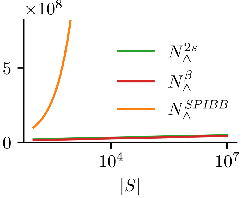
(a) $N_{\wedge}^{\text{SPIBB}},N_{\wedge}^{\mathsf{2s}}$ and $N_{\wedge}^{\beta}$.

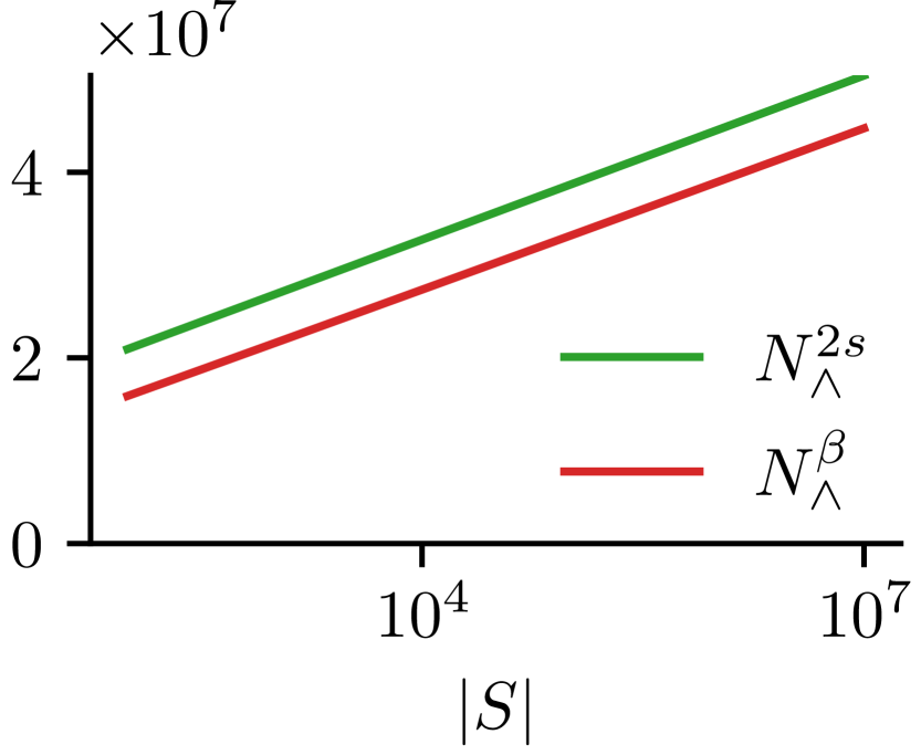
(b) $N_{\wedge}^{\mathsf{2s}}$ and $N_{\wedge}^{\beta}$.

Figure 3: Required number of samples for different $|S|$ with $|A|=4,V_{max}=1,\gamma=0.95,\delta=0.1$ and $\zeta=0.1$.

6 Implementation and Evaluation

We provide an evaluation of our approach from two different perspectives. First, a theoretical evaluation of how the different $N_{\wedge}$ depend on the size of a hypothetical MDP, and second, a practical evaluation to investigate how smaller $N_{\wedge}$ values translate to the performance of the improved policies.

6.1 Example Comparison of Different $N_{\wedge}$

To render the theoretical differences between the possible $N_{\wedge}$ discussed at the end of Section 5 more tangible, we now give a concrete example. We assume a hypothetical MDP with $|A|=4$, $V_{max}=1$, $\gamma=0.95$, and SPIBB parameters $\delta=0.1$ and $\zeta=0.1$. For varying sizes of the state-space, we compute all three sample size constraints: $N_{\wedge}^{\text{SPIBB}}$, $N_{\wedge}^{\mathsf{2s}}$, and $N_{\wedge}^{\beta}$. The results are shown in Figure 3, where Figure 3(a) shows the full plot and Figure 3(b) provides an excerpt to differentiate between the $N_{\wedge}^{\mathsf{2s}}$ and $N_{\wedge}^{\beta}$ plots by scaling down the $y$-axis. Note that the $x$-axis, the number of states in our hypothetical MDP, is on a log-scale. We see that $N_{\wedge}^{\text{SPIBB}}$ grows linearly with the number of states, whereas $N_{\wedge}^{\mathsf{2s}}$ and $N_{\wedge}^{\beta}$ are logarithmic in the number of states. Further, we note that $N_{\wedge}^{\beta}$ is significantly below $N_{\wedge}^{\mathsf{2s}}$, which follows from Lemma 1. Finally, the difference between $N_{\wedge}^{\text{SPIBB}}$ and $N_{\wedge}^{\mathsf{2s}}$ is for small MDPs of around a hundred states already a factor $10$.

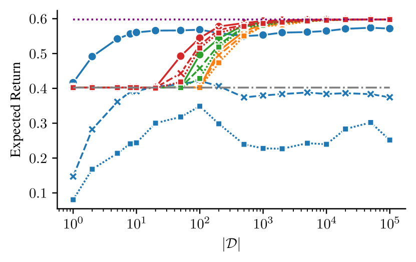
(a) $N_{\wedge}^{\text{SPIBB}}\!=\!100,N_{\wedge}^{\mathsf{2s}}\!=\!55,N_{\wedge}^{\beta}\!=\!27$.

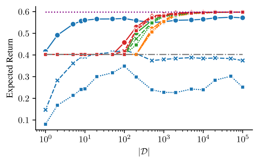
(b) $N_{\wedge}^{\text{SPIBB}}\!=\!200,N_{\wedge}^{\mathsf{2s}}\!=\!110,N_{\wedge}^{\beta}\!=\!67$.

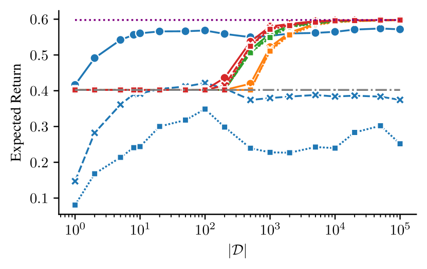
(c) $N_{\wedge}^{\text{SPIBB}}\!=\!400,N_{\wedge}^{\mathsf{2s}}\!=\!219,N_{\wedge}^{\beta}\!=\!146$.

Figure 4: Safe policy improvement on the Gridworld environment.

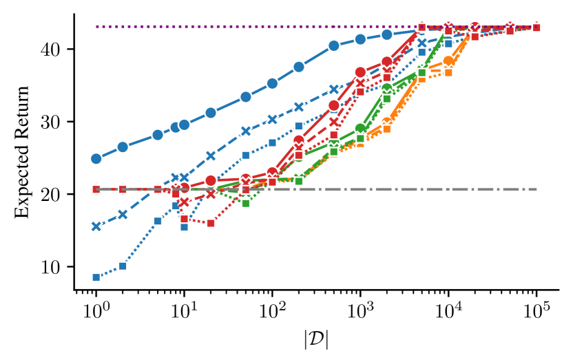
(a) $N_{\wedge}^{\text{SPIBB}}\!=\!60,N_{\wedge}^{\mathsf{2s}}\!=\!34,N_{\wedge}^{\beta}\!=\!10$.

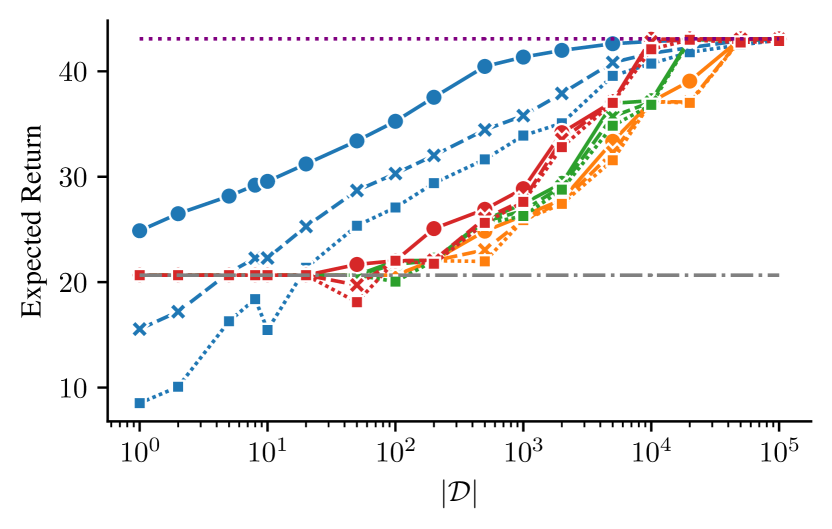
(b) $N_{\wedge}^{\text{SPIBB}}\!=\!120,N_{\wedge}^{\mathsf{2s}}\!=\!67,N_{\wedge}^{\beta}\!=\!36$.

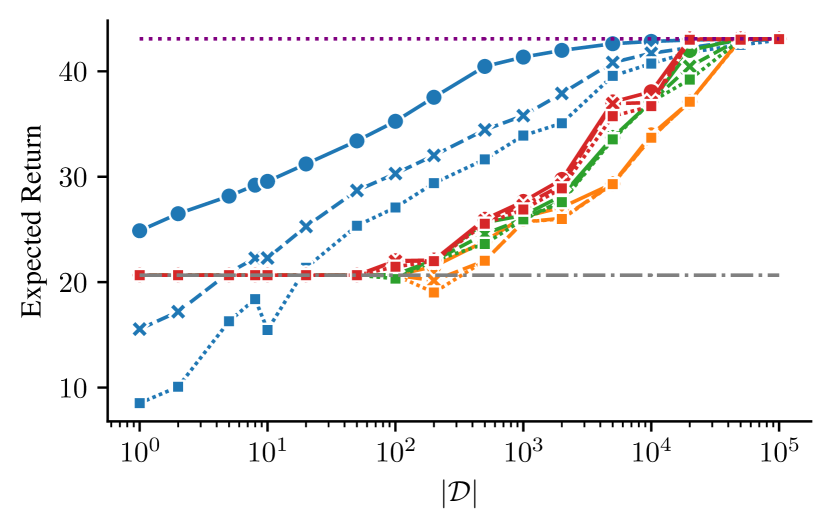
(c) $N_{\wedge}^{\text{SPIBB}}\!=\!180,N_{\wedge}^{\mathsf{2s}}\!=\!101,N_{\wedge}^{\beta}\!=\!61$.

Figure 5: Safe policy improvement on the Wet Chicken environment.

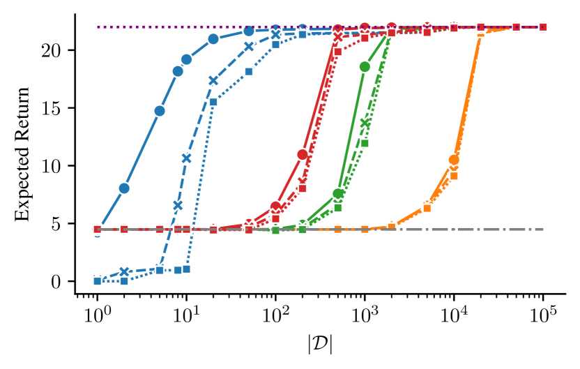
(a) $N_{\wedge}^{\text{SPIBB}}\!=\!600,N_{\wedge}^{\mathsf{2s}}\!=\!43,N_{\wedge}^{\beta}\!=\!12$.

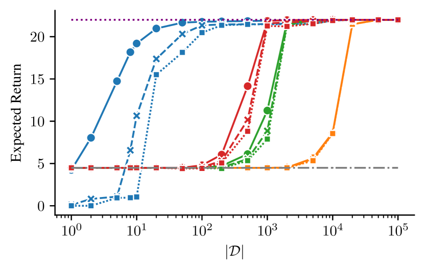
(b) $N_{\wedge}^{\text{SPIBB}}\!=\!800,N_{\wedge}^{\mathsf{2s}}\!=\!57,N_{\wedge}^{\beta}\!=\!25$.

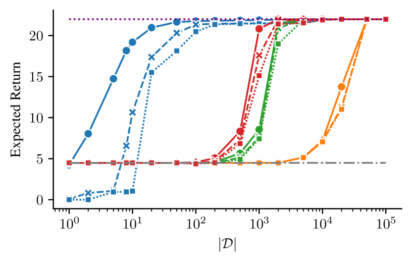
(c) $N_{\wedge}^{\text{SPIBB}}\!=\!1000,N_{\wedge}^{\mathsf{2s}}\!=\!71,N_{\wedge}^{\beta}\!=\!37$.

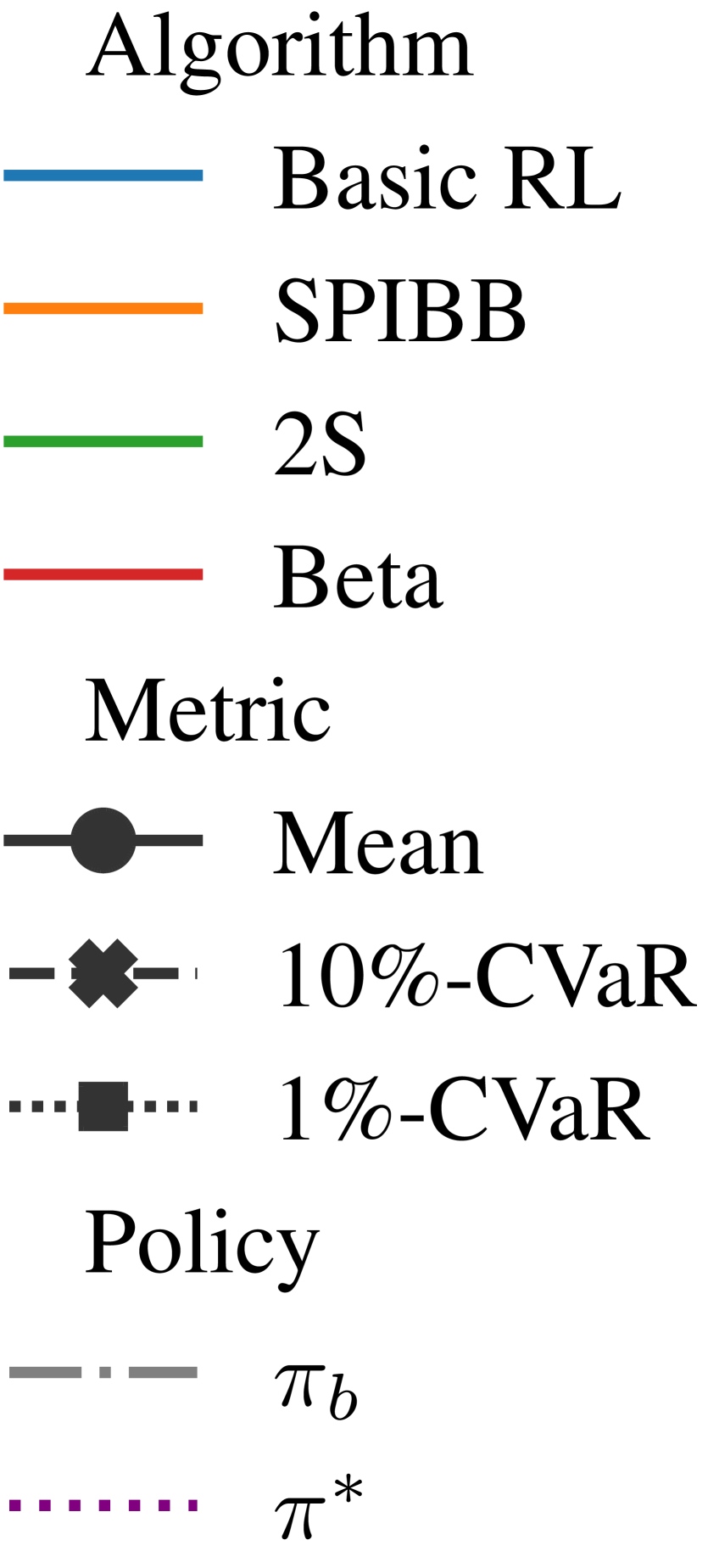
Figure 6: Safe policy improvement on the Resource Gathering environment.

6.1.1 Discussion.

While we show that a significant reduction of the required number of samples per state-action pair $N_{\wedge}$ is possible via our two approaches, we note that even for small MDPs (e.g., $|S|=100$) we still need over $10$ million samples per state-action pair to guarantee that an improved policy is safe w.r.t. the behavior policy. That is, with probability $1-\delta=0.9$, an improved policy will have an admissible performance loss of at most $\zeta=0.1$, which is infeasible in practice. Nevertheless, a practical evaluation of our approaches is possible taking on a different perspective, which we address in the next section.

6.2 Evaluation in SPIBB

We integrate our novel results for computing $\zeta^{\mathsf{2s}},\zeta^{\beta},N_{\wedge}^{\mathsf{2s}}$, and $N_{\wedge}^{\beta}$ into the implementation of SPIBB Laroche et al. (2019).

Benchmarks.

We consider two standard benchmarks used in SPI and one other well-known MDP: the $25$-state Gridworld proposed by Laroche et al. (2019), the $25$-state Wet Chicken benchmark Hans and Udluft (2009), which was used to evaluate SPI approaches by Scholl et al. (2022), and a $376$-state instance of Resource Gathering proposed by Barrett and Narayanan (2008).

Behavior policy.

For the Gridworld, we use the same behavior policy as Laroche et al. (2019). For the Wet Chicken environment, we use Q-Learning with a softmax function to derive a behavior policy. The behavior policy of Resource Gathering was derived from the optimal policy by selecting each non-optimal action with a probability of 1e-5.

Methodology.

Recall that in the standard SPIBB approach, $N_{\wedge}$ is used as a hyperparameter, since the actual $N_{\wedge}$ for reasonable $\delta$ and $\zeta$ are infeasible. While our methods improve significantly on $N_{\wedge}$, the values we obtain are still infeasible in practice, as discussed in Section 6.1. We still use $N_{\wedge}^{\text{SPIBB}}$ as a hyperparameter, and then run the SPIBB algorithm and compute the resulting $\zeta^{\text{SPIBB}}$. This $\zeta^{\text{SPIBB}}$ is consequently used to compute the values $N_{\wedge}^{\mathsf{2s}}$ and $N_{\wedge}^{\beta}$ that ensure the same performance loss. We then run SPIBB again with these two values for $N_{\wedge}$. As seen in the previous experiment, and detailed at the end of Section 5, for most MDPs – including our examples – we have $N_{\wedge}^{\beta}\leq N_{\wedge}^{\mathsf{2s}}\leq N_{\wedge}^{\text{SPIBB}}$ for a fixed $\zeta$.

Evaluation metrics.

For each data set size, we repeat each experiment $1000$ times and report the mean performance of the learned policy, as well as the $10\%$ and $1\%$ conditional value at risk (CVaR) values Rockafellar et al. (2000), indicating the mean performance of the worst $10\%$ and $1\%$ runs. To give a complete picture, we also include the performance of basic RL (dynamic programming on the MLE-MDP Sutton and Barto (1998)), the behavior policy $\pi_{b}$, and the optimal policy $\pi^{*}$ of the underlying MDP.

6.2.1 Results.

We present the results for the Gridworld, Wet Chicken, and Resource Gathering environments for three different hyperparameters $N_{\wedge}^{\text{SPIBB}}$ in Figures 4, 5, and 6, respectively. In all instances, we see similar and improved behaviors as we presumed by sharpening the sampling bounds with our new approaches. Smaller values for $N_{\wedge}$ typically require smaller data sets for a policy to start improving, and this is precisely what our methods set out to do. In particular, we note that our methods (2S and Beta) are quicker to converge to an optimal policy than standard SPIBB. Beta is, as expected, the fastest, and starts to improve over the behavior policy for data sets about half the size compared to SPIBB in the Gridworld. Further, while theoretically, the factor between the different $N_{\wedge}$ does not directly translate to the whole data set size, we see that in practice on all three benchmarks this is roughly the case. Finally, we note that Basic RL is unreliable compared to the SPI methods, as seen by the CVaR values being significantly below the baseline performance for several data set sizes in all three environments. This is as expected and in accordance with well-established results.

7 Related Work

A variant of our transformation from MDP to 2sMDP was introduced by Mayr and Munday Mayr and Munday (2023), utilizing binary trees built from auxiliary states as gadgets. Similar to our construction, Junges et al. Junges et al. (2018) transform a partially observable MDP (POMDP) Kaelbling et al. (1998); Spaan (2012) into a simple POMDP, where each state has either one action choice, and an arbitrary number of successor states, or where there are multiple actions available but each action has a single successor state. The same transformation was applied to uncertain POMDPs Cubuktepe et al. (2021).

Besides the main approaches to SPI mentioned in Section 3, there are a number of other noteworthy works in this area. SPIBB has been extended to soft baseline bootstrapping in Nadjahi et al. (2019), where instead of either following the behavior policy or the optimal policy in the MLE-MDP in a state-action pair, randomization between the two is applied. However, the theoretical guarantees of this approach rely on an assumption that rarely holds Scholl et al. (2022).

Incorporating structural knowledge of the environment has been shown to improve the sample complexity of SPI algorithms Simão and Spaan (2019a, b). It is also possible to deploy the SPIBB algorithm in problems with large state space using MCTS Castellini et al. (2023). For a more detailed overview of SPI approaches and an empirical comparison between them, see Scholl et al. (2022). For an overview of how these algorithms scale in the number of states, we refer to Brandfonbrener et al. (2022).

Other related work investigated how to relax some of the assumptions SPI methods make. In Simão et al. (2020), a method for estimating the behavior policy is introduced, relaxing the need to know this policy. Finally, a number of recent works extend the scope and relax common assumptions by introducing SPI in problems with partial observability Simão et al. (2023), non-stationary dynamics Chandak et al. (2020), and multiple objectives Satija et al. (2021).

Finally, we note that SPI is a specific offline RL problem Levine et al. (2020) and there have been significant advances in the general offline setting recently Kidambi et al. (2020); Yu et al. (2020); Kumar et al. (2020); Smit et al. (2021); Yu et al. (2021); Rigter et al. (2022). While these approaches may be applicable to high dimensional problems such as control tasks and problems with large observation space Fu et al. (2020), they often ignore the inherent reliability aspect of improving over a baseline policy, as SPI algorithms do. Nevertheless, it remains a challenge to bring SPI algorithms to high-dimensional problems.

8 Conclusion

We presented a new approach to safe policy improvement that reduces the required size of data sets significantly. We derived new performance guarantees and applied them to state-of-the-art approaches such as SPIBB. Specifically, we introduced a novel transformation to the underlying MDP model that limits the branching factor, and provided two new ways of computing the admissible performance loss $\zeta$ and the sample size constraint $N_{\wedge}$, both exploiting the limited branching factor in SPI(BB). This improves the overall performance of SPI algorithms, leading to more efficient use of a given data set.

Appendix A Proofs

Proof Theorem 1.

Fix a state $s\in S$ and action $a\in A$ that is enabled in $s$ and assume $\mathit{Post}_{M}(s,a)=\{s_{1},\dots,s_{k}\}$. We define $p_{i}=P(s_{i}\,|\,s,a)$ for all $i=1,\dots,k$.

By definition, for each $s_{i}\in\mathit{Post}_{M}(s,a)$ with $i<k$ a path $\langle s,a,x_{2},\tau,\dots,x_{i},\tau,s_{i}\rangle$ and has positive probability. For $i=k$ the path is $\langle s,a,x_{2},\tau,\dots,x_{k-1},\tau,s_{k}\rangle$ instead. Note that there is exactly one incoming transition for each auxiliary state $x_{i}\in S_{\text{aux}}^{s,a}$ and each $s_{i}\in\mathit{Post}_{M}(s,a)$ has exactly one predecessor in $S_{\text{aux}}^{s,a}$. Further, $\mathit{Post}_{M^{\mathsf{2s}}}(s,a)\subseteq S_{\text{aux}}^{s,a}\cup\mathit{Post}_{M}(s,a)$ and also $\mathit{Post}_{M^{\mathsf{2s}}}(x,\tau)\subseteq S_{\text{aux}}^{s,a}\cup\mathit{Post}_{M}(s,a)$ for all $x\in S_{\text{aux}}^{s,a}$, i.e., any path $\langle s,a,\dots\rangle$ must stay in the set $S_{\text{aux}}^{s,a}$ until it reaches a state in $\mathit{Post}_{M}(s,a)$. Thus the path from $s$ to $s_{i}$ must be unique.

We now show that the probabilities pre- and post-transformation match, i.e., $\mathbb{P}_{M}(\langle s,a,s_{i}\rangle)=\mathbb{P}_{{M^{\mathsf{2s}}}}(\langle s,a,x_{2},\tau,\dots,x_{i},\tau,s_{i}\rangle)$. For $s_{i}=s_{1}$ the statement holds by definition. Now, consider the case $2\leq i\leq k-1$. Then we can compute the probability of the path as

$$\mathbb{P}_{{M^{\mathsf{2s}}}}(\langle s,a,x_{2},\tau,\dots,x_{i},\tau,s_{i}\rangle) =P^{\mathsf{2s}}(x_{2}\,|\,s,a)\left(\prod_{j=2}^{i-1}P^{\mathsf{2s}}(x_{j+1}\,|\,x_{j},\tau)\right)P^{\mathsf{2s}}(s_{i}\,|\,x_{i},\tau)$$

$$=(1-p_{1})\left(\prod_{j=2}^{i-1}1-\frac{p_{j}}{1-(p_{1}+\dots+p_{j-1})}\right)\frac{p_{i}}{1-(p_{1}+\dots+p_{i-1})}$$

$$=(1-p_{1})\left(\prod_{j=2}^{i-1}\frac{1-(p_{1}+\dots+p_{j})}{1-(p_{1}+\dots+p_{j-1})}\right)\frac{p_{i}}{1-(p_{1}+\dots+p_{i-1})}$$

$$=p_{i}$$

$$=\mathbb{P}_{M}(\langle s,a,s_{i}\rangle).$$

For the case $i=k$ the proof is analogous to the case $i=k-1$, replacing the last factor by $P^{\mathsf{2s}}(s_{k}\,|\,x_{k-1},\tau)$. ∎

Proof Corollary 1.

Recall that the auxiliary states can only choose action $\tau$ which does not yield any reward. Further, since no discount is applied in auxiliary states, for all states $s\in S$ we have

$$V_{M^{\mathsf{2s}}}^{\pi^{\mathsf{2s}}}(s)\ =\ \sum\limits_{a\in A}{\pi^{\mathsf{2s}}}(a\,|\,s)\Big{(}R^{\mathsf{2s}}(s,a)+\gamma^{\mathsf{2s}}(s)\sum\limits_{s^{\prime}\in S}P^{\mathsf{2s}}(s^{\prime}\,|\,s,a)V_{M^{\mathsf{2s}}}^{\pi^{\mathsf{2s}}}(s^{\prime})\Big{)}$$

$$=\ \sum\limits_{a\in A}\pi(a\,|\,s)\Big{(}R(s,a)+\gamma\sum\limits_{s^{\prime}\in S}\mathbb{P}_{{M^{\mathsf{2s}}}}(s_{i}\,|\,s,a,x_{2},\tau,\dots,x_{i},\tau)V_{M^{\mathsf{2s}}}^{\pi^{\mathsf{2s}}}(s^{\prime})\Big{)}$$

$$=\ \sum\limits_{a\in A}\pi(a\,|\,s)\Big{(}R(s,a)+\gamma\sum\limits_{s^{\prime}\in S}P(s,a)V_{M^{\mathsf{2s}}}^{\pi^{\mathsf{2s}}}(s^{\prime})\Big{)}.$$

This is exactly the defining Bellman equation for $V_{m}^{\pi}$, i.e., by definition, we have

$$V_{m}^{\pi}(s)=\sum\limits_{a\in A}\pi(a\,|\,s)\Big{(}R(s,a)+\gamma\sum\limits_{s^{\prime}\in S}P(s,a)V_{M}^{\pi}(s^{\prime})\Big{)}.$$

As the Bellman equation has a unique fixed point for a discount factor $\gamma<1$ (see e.g. Sutton and Barto [1998]), we must have $V_{m}^{\pi}=V_{M^{\mathsf{2s}}}^{\pi^{\mathsf{2s}}}(s)$ for all $s\in S$. In particular, this holds for $s=\iota$, and thus $\rho(M,\pi)=\rho({M^{\mathsf{2s}}},{\pi^{\mathsf{2s}}})$ ∎

Proof Theorem 2.

The proof is similar to the proof of Theorem 1.

Again, fix a state $s\in S$ and action $a\in A$ that is enabled in $s$ and assume $\mathit{Post}_{{\tilde{M}}}(s,a)=\{s_{1},\dots,s_{k}\}$. For the case $k\leq 2$ the statement trivially holds as $\#_{\mathcal{D}}(s,a,\cdot)=\#_{\mathcal{D}^{\mathsf{2s}}}(s,a,\cdot)$. We now consider the case $k>2$.

As we have $\tilde{P}^{\mathsf{2s}}(s^{\prime}\,|\,s,a)>0$ if and only if $\#_{\mathcal{D}^{\mathsf{2s}}}(s,a,s^{\prime})>0$ for all $s,s^{\prime}\in S\cup S_{\text{aux}}$, and for each $s^{\prime}\in S_{\text{aux}}^{s,a}\cup\mathit{Post}_{{\tilde{M}}}(s,a)$ by definition there is exactly one state $s\in S_{\text{aux}}^{s,a}\cup\{s\}$ for which $\#_{\mathcal{D}^{\mathsf{2s}}}(s,a,s^{\prime})>0$, there for each $i\in\{1,\dots,k\}$ must be exactly one unique path $\langle s,a,x_{2},\tau,\dots,x_{i},\tau,s_{i}\rangle$ in ${\tilde{M}^{\mathsf{2s}}}$.

We now show that $\mathbb{P}_{{\tilde{M}}}(\langle s,a,s_{i}\rangle)=\mathbb{P}_{{\tilde{M}^{\mathsf{2s}}}}(\langle s,a,x_{2},\tau,\dots,x_{i},\tau,s_{i}\rangle)$. For $s_{i}=s_{1}$ the statement holds by definition. Now consider the case $2\leq i\leq k-1$. Then we can compute the probability of the path as

$$\mathbb{P}_{{\tilde{M}^{\mathsf{2s}}}}(\langle s,a,x_{2},\tau,\dots,x_{i},\tau,s_{i}\rangle) =P_{\tilde{M}^{\mathsf{2s}}}(x_{2}\,|\,s,a)\left(\prod_{j=2}^{i-1}P_{\tilde{M}^{\mathsf{2s}}}(x_{j+1}\,|\,x_{j},\tau)\right)P_{\tilde{M}^{\mathsf{2s}}}(s_{i}\,|\,x_{i},\tau)$$

$$=\frac{\#_{\mathcal{D}^{\mathsf{2s}}}(s,a,x_{2})}{\sum_{s^{\prime}}\#_{\mathcal{D}^{\mathsf{2s}}}(s,a,s^{\prime})}\left(\prod_{j=2}^{i-1}\frac{\#_{\mathcal{D}^{\mathsf{2s}}}(x_{i},\tau,x_{j+1})}{\sum_{s^{\prime}}\#_{\mathcal{D}^{\mathsf{2s}}}(x_{j},\tau,s^{\prime})}\right)\frac{\#_{\mathcal{D}^{\mathsf{2s}}}(x_{i},\tau,s_{i})}{\sum_{s^{\prime}}\#_{\mathcal{D}^{\mathsf{2s}}}(x_{i},\tau,s^{\prime})}$$

$$=\frac{\#_{\mathcal{D}^{\mathsf{2s}}}(s,a,x_{2})}{\#_{\mathcal{D}^{\mathsf{2s}}}(s,a,s_{1})+\#_{\mathcal{D}^{\mathsf{2s}}}(s,a,x_{2})}\left(\prod_{j=2}^{i-1}\frac{\#_{\mathcal{D}^{\mathsf{2s}}}(x_{i},\tau,x_{j+1})}{\#_{\mathcal{D}^{\mathsf{2s}}}(x_{j},\tau,s_{j})+\#_{\mathcal{D}^{\mathsf{2s}}}(x_{j},\tau,x_{j+1})}\right)$$

$$\phantom{==}\frac{\#_{\mathcal{D}^{\mathsf{2s}}}(x_{i},\tau,s_{i})}{\#_{\mathcal{D}^{\mathsf{2s}}}(x_{i},\tau,s_{i})+\#_{\mathcal{D}^{\mathsf{2s}}}(x_{i},\tau,x_{i+1})}$$

$$=\frac{\sum_{m=2}^{k}\#_{\mathcal{D}}(s,a,s_{m})}{\#_{\mathcal{D}}(s,a,s_{1})+\sum_{m=2}^{k}\#_{\mathcal{D}}(s,a,s_{m})}\left(\prod_{j=2}^{i-1}\frac{\sum_{m=j+1}^{k}\#_{\mathcal{D}}(s,a,s_{m})}{\#_{\mathcal{D}}(s,a,s_{j})+\sum_{m=j+1}^{k}\#_{\mathcal{D}}(s,a,s_{m})}\right)$$

$$\phantom{==}\frac{\#_{\mathcal{D}}(s,a,s_{i})}{\#_{\mathcal{D}}(s,a,s_{i})+\sum_{m=i+1}^{k}\#_{\mathcal{D}}(s,a,s_{m})}$$

$$=\frac{\sum_{m=2}^{k}\#_{\mathcal{D}}(s,a,s_{m})}{\sum_{m=1}^{k}\#_{\mathcal{D}}(s,a,s_{m})}\left(\prod_{j=2}^{i-1}\frac{\sum_{m=j+1}^{k}\#_{\mathcal{D}}(s,a,s_{m})}{\sum_{m=j}^{k}\#_{\mathcal{D}}(s,a,s_{m})}\right)\frac{\#_{\mathcal{D}}(s,a,s_{i})}{\sum_{m=i}^{k}\#_{\mathcal{D}}(s,a,s_{m})}$$

$$=\frac{\#_{\mathcal{D}}(s,a,s_{i})}{\sum_{m=1}^{k}\#_{\mathcal{D}}(s,a,s_{m})}$$

$$=\frac{\#_{\mathcal{D}}(s,a,s_{i})}{\sum_{s^{\prime}}\#_{\mathcal{D}}(s,a,s^{\prime})}$$

$$=\mathbb{P}_{\tilde{M}}(s_{i}\,|\,s,a).$$

The case where $i=k$ is analogous to the case $i=k-1$. ∎

Proof Corollary 2.

Using Theorem 2, the proof is analogous to the proof of Corollary 1. ∎

Proof Lemma 1.

The proof follows a similar argumentation as [Laroche et al., 2019, Theorem 2]. First, note that we cannot directly apply the cited theorem as we deal with a two-successor MDP for which $\rho(\cdot,\cdot)$ is defined in a different manner. More precisely, the discount rate $\gamma$ is not constant. We now show that the results can still be applied in our setting by adapting the proof of [Laroche et al., 2019, Theorem 2].

Let ${M^{\mathsf{2s}}}=(S\cup S_{\text{aux}},A\cup\{\tau\},P^{\mathsf{2s}},R^{\mathsf{2s}},\gamma)$ be the given two-successor MDP, $\mathcal{D}$ a data-set of trajectories over ${M^{\mathsf{2s}}}$ and $N_{\wedge}\in\mathbb{N}$ a given parameter. The set of bootstrapped state-action pairs is defined as $\mathcal{U}=\{(s,a)\mid\#_{{\mathcal{D}^{\mathsf{2s}}}}(s,a)<N_{\wedge}\}\cup\{(s,\tau)\mid s\in S\}$. Note that actions in auxiliary states are always bootstrapped. The behavior policy $\pi_{b}$ is decomposed into $\tilde{\pi}_{b}$, for bootstrapped actions, and $\dot{\pi}_{b}$, for non-bootstrapped actions, i.e.,

$$\tilde{\pi}_{b}=\begin{cases}\pi_{b}(a\,|\,s)&(a\,|\,s)\in\mathcal{U}\\ 0&\text{else}\end{cases}$$

and $\dot{\pi}_{b}(a\,|\,s)=\pi_{b}(a\,|\,s)-\tilde{\pi}_{b}(a\,|\,s)$.

We now transform ${M^{\mathsf{2s}}}$ into a its corresponding bootstrapped semi-MDP Sutton and Barto [1998] counterpart $\ddot{M}$. Precisely, $\ddot{M}=(S\cup S_{\text{aux}},\Omega_{A},\ddot{P},\ddot{R},\Gamma)$ with $\Omega_{A}=\{\omega_{a}\}_{a\in A}$ where for each $a\in A$

$$\omega_{a}=\langle I_{a},a:\pi_{b},\beta(s)\rangle\begin{cases}I_{a}=\{s\mid(s,a)\not\in\mathcal{U}\}\\ a:\pi_{b}\dots\text{choose $a$, then follow $\pi_{b}$}\\ \beta(s)=\sum_{a^{\prime}\in A\cup\{\tau\}}{\dot{\pi}_{b}(s,a^{\prime})}\end{cases}$$

and

$$\Gamma(s,a)=\begin{cases}\gamma&s\in S\\ 1&s\in S_{\text{aux}}\end{cases}$$

$P$ and $R$ are naturally extended to options, i.e., $\ddot{P}(s,\omega_{a})=P^{2s}(s,a)$ and $\ddot{R}(s,\omega_{a})=R^{2s}(s,a)$. In the same fashion we transform the MLE MDP ${\tilde{M}^{\mathsf{2s}}}$ into its bootstrapped counterpart $\tilde{\ddot{M}}^{2s}=(S\cup S_{\text{aux}},\Omega_{A},\tilde{\ddot{P}},\ddot{R},\Gamma)$.

Using Theorem 2.1 from Weissman et al. [2003] on all $(s,a)\not\in\mathcal{U}$ we obtain that for all $a\in A$ and $s\in I_{a}$, with probability at least $1-\delta$ we have

$$\lVert\gamma\ddot{P}(s,a)-\gamma\tilde{\ddot{P}}(s,a)\rVert_{1} \leq\sqrt{\frac{2}{\min_{a\in A,s\in I_{a}}\#_{{\mathcal{D}^{\mathsf{2s}}}}(s,a)}\log\frac{2|S||A|2^{\max_{a\in A,s\in I_{a}}|\mathit{Post}(s,a)|}}{\delta}}$$

$$\leq\sqrt{\frac{2}{N_{\wedge}}\log\frac{8|S||A|}{\delta}}$$

This means we can apply Lemma 1 from Laroche et al. [2019] to ${M^{\mathsf{2s}}}$ and ${\tilde{M}^{\mathsf{2s}}}$ for arbitrary bootstrapped policies to obtain

$$|\rho(\pi^{\mathsf{2s}}_{\odot},{M^{\mathsf{2s}}})-\rho(\pi^{\mathsf{2s}}_{\odot},{\tilde{M}^{\mathsf{2s}}})| \leq\frac{2V_{max}}{1-\gamma}\sqrt{\frac{2}{N_{\wedge}}\log\frac{8|S||A|}{\delta}}$$

$$|\rho(\pi^{\mathsf{2s}}_{b},{M^{\mathsf{2s}}})-\rho(\pi^{\mathsf{2s}}_{b},{\tilde{M}^{\mathsf{2s}}})| \leq\frac{2V_{max}}{1-\gamma}\sqrt{\frac{2}{N_{\wedge}}\log\frac{8|S||A|}{\delta}}$$

Combining these inequalities we obtain the final result

$$\zeta^{2s} =\rho(\pi^{\mathsf{2s}}_{b},{M^{\mathsf{2s}}})-\rho(\pi^{\mathsf{2s}}_{\odot},{M^{\mathsf{2s}}})$$

$$\leq\frac{4V_{max}}{1-\gamma}\sqrt{\frac{2}{N_{\wedge}}\log\frac{8|S||A|}{\delta}}-\rho(\pi^{\mathsf{2s}}_{\odot},{\tilde{M}^{\mathsf{2s}}})+\rho(\pi^{\mathsf{2s}}_{b},{\tilde{M}^{\mathsf{2s}}}).\qed$$

Proof Theorem 3.

$$\rho(\pi_{\odot},M) =\rho(\pi^{\mathsf{2s}}_{\odot},{M^{\mathsf{2s}}})$$

$$\geq\rho(\pi_{b}^{\mathsf{2s}},{M^{\mathsf{2s}}})-\frac{4V_{max}}{1-\gamma}\sqrt{\frac{2}{N_{\wedge}}\log\frac{8\lvert S\rvert^{2}\lvert A\rvert^{2}}{\delta}}-\rho(\pi^{\mathsf{2s}}_{\odot},{\tilde{M}^{\mathsf{2s}}})+\rho(\pi_{b}^{\mathsf{2s}},{\tilde{M}^{\mathsf{2s}}})$$

$$=\rho(\pi_{b},M)-\zeta^{\mathsf{2s}}$$

Both equalities follow by applying Theorem 1 and Theorem 2. The inequality is obtained by applying Lemma 1 to ${M^{\mathsf{2s}}}$ where the size of the state space of ${M^{\mathsf{2s}}}$ is bounded by $|S\cup S_{\text{aux}}|\leq|S|^{2}|A|$ (cf. Section 4.1). ∎

$k$-successor MDPs.

We saw that the $N_{\wedge}^{\text{SPIBB}}$ grows linearly in $|S|$ whereas $N_{\wedge}^{\mathsf{2s}}$ grows logarithmically in $|S|$. The contributing factor to this was that for any state-action pair $(s,a)$ the $L_{1}$-norm between the true successor distribution $P(s,a)$ and its maximum likelihood estimate can only be bounded linearly in terms of the branching factor $k=|\mathit{Post}(s,a)|$ when applying the bound obtained by Weissman et al. [2003]. Hence, the idea behind our 2sMDP transformation was to bound the branching factor by a constant. To achieve this, we necessarily needed to introcude auxiliary state, essentially creating a trade-off between branching factor and size of the state space. One question that may arise is whether it may be beneficial to allow for a larger branching factor $k$ than $2$, possibly harvesting the advantage of having to introduce less auxiliary states. In Section 4.1 we hint at the fact that for SPI algorithms, $k=2$ is indeed optimal. We now outline why this is the case.

First, notice that we can easily adapt the transformation outlined in Section 4.1 towards $k$-successor MDPs by structuring the auxiliary nodes in a tree with branching factor $2$ rather than in a binary tree, resulting in up to $\nicefrac{{|S|}}{{k-1}}$ auxiliary states in each tree. Thus, when transforming an arbitrary MDP into a $k$-successor MDP, we can bound the $L_{1}$-error in the same fashion as in Theorem 3 to obtain

$$N_{\wedge}^{ks}=\frac{32V_{max}^{2}}{\zeta^{2}(1-\gamma)^{2}}\log\frac{2\lvert S\rvert^{2}\lvert A\rvert^{2}2^{k}}{(k-1)\delta}$$

As all terms are positive his expression is minimal if and only if $\frac{2^{k}}{k-1}$ is minimal, which is the case for $k=2$ and $k=3$. Hence, 2sMDP are optimal for SPIBB when utilizing the $L_{1}$-norm bound by Weissman et al. [2003].

The main reason why we choose a branching factor of $k=2$ over $k=3$ is that for $k=2$ we can give even tighter bounds on the $L_{1}$-norm by computing integrals over the pdf of the transition probabilities that is given by a beta distribution as described in Section 5.1. Next, we provide proofs for the Lemma and Theorem in that section.

Proof Lemma 2.

We first show that for $k=\frac{n}{2}$ the statement holds.

Let $B(\cdot,\cdot)$ denote the beta function and $f_{B}(\cdot;a,b)$ the probability density function of the Beta distribution with parameters $a$ and $b$.

Consider the interval $[\underline{p},\overline{p}]=[\frac{1}{2}-h,\frac{1}{2}+h]$ with $h=\frac{1}{2}\left(1-2I_{\nicefrac{{\delta_{T}}}{{2}}}^{-1}\left(\frac{n}{2}+1,\frac{n}{2}+1\right)\right)$. The interval clearly has size $\overline{p}-\underline{p}=1-2I_{\nicefrac{{\delta_{T}}}{{2}}}^{-1}\left(\frac{n}{2}+1,\frac{n}{2}+1\right)$. Now we show that it contains $p$ with probability $1-\delta_{T}$.

$$\mathbb{P}\left(p\in\left[\underline{p},\overline{p}\right]\right) =\int_{\frac{1}{2}-h}^{\frac{1}{2}+h}f_{B}(u,\frac{n}{2}+1,\frac{n}{2}+1)$$ (3)

$$=\int_{\frac{1}{2}-h}^{\frac{1}{2}+h}\frac{u^{\frac{n}{2}}\left(1-u\right)^{\frac{n}{2}}}{B\left(\frac{n}{2}+1,\frac{n}{2}+1\right)}du$$ (4)

$$=I_{\frac{1}{2}+h}\left(\frac{n}{2}+1,\frac{n}{2}+1\right)-I_{\frac{1}{2}-h}\left(\frac{n}{2}+1,\frac{n}{2}+1\right)$$ (5)

$$=1-2\cdot I_{\frac{1}{2}-h}\left(\frac{n}{2}+1,\frac{n}{2}+1\right)$$ (6)

$$=1-2I_{I_{\nicefrac{{\delta_{T}}}{{2}}}^{-1}\left(\frac{n}{2}+1,\frac{n}{2}+1\right)}\left(\frac{n}{2}+1,\frac{n}{2}+1\right)$$ (7)

$$=1-2\frac{\delta_{T}}{2}$$ (8)

$$=1-\delta_{T}$$ (9)

Note that Equation 3 assumes a unform prior. Equation 5 is obtained by definition and Equation 6 by using the symmetry of $I(a,a)$.

Due to symmetry of $f_{B}(\cdot,\frac{n}{2},\frac{n}{2})$ and its monotonicity on the intervals $[0,\frac{1}{2})$ and $(\frac{1}{2},1]$ we have for all $r\in[0,\frac{1}{2}-h]\cup[\frac{1}{2}+h,1]$ and $s\in[\frac{1}{2}-h,\frac{1}{2}+h]$ that

$$f_{B}(r,\frac{n}{2},\frac{n}{2})\leq f_{B}(\frac{1}{2}-h,\frac{n}{2},\frac{n}{2})=f_{B}(\frac{1}{2}+h,\frac{n}{2},\frac{n}{2})\leq f_{B}(s,\frac{n}{2},\frac{n}{2})$$

Further, as $f_{B}(\cdot,\frac{n}{2},\frac{n}{2})$ is positive on $[0,1]$, we conclude that for any interval $[\underline{p}^{\prime},\overline{p}^{\prime}]$ with $\overline{p}^{\prime}-\underline{p}^{\prime}=\overline{p}-\underline{p}$ we have $\mathbb{P}\left(p\in\left[\underline{p}^{\prime},\overline{p}^{\prime}\right]\right)\leq\mathbb{P}\left(p\in\left[\underline{p},\overline{p}\right]\right)$. As all steps in the chain above are equalities, $\left[\underline{p},\overline{p}\right]$ is indeed the smallest interval for which we can guarantee $\mathbb{P}\left(p\in\left[\underline{p},\overline{p}\right]\right)\geq 1-\delta_{T}$.

Next, we consider arbitrary $1\leq k\leq n-1$. In this case we construct the following interval which contains $p$ with probability $1-\delta_{T}$ by definition:

$$\left[\underline{p}_{k},\overline{p}_{k}\right]=[I^{-1}_{\nicefrac{{\delta_{T}}}{{2}}}(k,n-k),I^{-1}_{1-\nicefrac{{\delta_{T}}}{{2}}}(k,n-k)]$$

Note that for $k=\nicefrac{{n}}{{2}}$ the intervals $\left[\underline{p},\overline{p}\right]$ and $\left[\underline{p}_{k},\overline{p}_{k}\right]$ coincide.

We now show that the size of the interval $\overline{p}_{k}-\underline{p}_{k}$ is maximal if $k=\nicefrac{{n}}{{2}}$. We do this by computing the derivative with respect to k. Substituting $a=k$ and $b=n-k$, using symmetry, applying the multi-variable chain rule, and renaming integration variables we obtain

$$\frac{\partial}{\partial k}(I^{-1}_{1-\nicefrac{{\delta_{T}}}{{2}}}(k,n-k)-I^{-1}_{\nicefrac{{\delta_{T}}}{{2}}}(k,n-k))$$

$$=\frac{\partial}{\partial k}(I^{-1}_{1-\nicefrac{{\delta_{T}}}{{2}}}(a,b)-I^{-1}_{\nicefrac{{\delta_{T}}}{{2}}}(a,b))$$

$$=\frac{\partial}{\partial k}(1-I^{-1}_{\nicefrac{{\delta_{T}}}{{2}}}(b,a)-I^{-1}_{\nicefrac{{\delta_{T}}}{{2}}}(a,b))$$

$$=\frac{\partial}{\partial b}I^{-1}_{\nicefrac{{\delta_{T}}}{{2}}}(b,a)-\frac{\partial}{\partial a}I^{-1}_{\nicefrac{{\delta_{T}}}{{2}}}(b,a)-\frac{\partial}{\partial a}I^{-1}_{\nicefrac{{\delta_{T}}}{{2}}}(a,b)+\frac{\partial}{\partial b}I^{-1}_{\nicefrac{{\delta_{T}}}{{2}}}(a,b)$$

$$=\frac{\partial}{\partial c}I^{-1}_{\nicefrac{{\delta_{T}}}{{2}}}(c,a)-\frac{\partial}{\partial c}I^{-1}_{\nicefrac{{\delta_{T}}}{{2}}}(b,c)-\frac{\partial}{\partial c}I^{-1}_{\nicefrac{{\delta_{T}}}{{2}}}(c,b)+\frac{\partial}{\partial c}I^{-1}_{\nicefrac{{\delta_{T}}}{{2}}}(a,c)$$

$$=\frac{\partial}{\partial c}\left(I^{-1}_{\nicefrac{{\delta_{T}}}{{2}}}(c,a)-I^{-1}_{\nicefrac{{\delta_{T}}}{{2}}}(c,b)\right)-\frac{\partial}{\partial c}\left(I^{-1}_{\nicefrac{{\delta_{T}}}{{2}}}(b,c)-I^{-1}_{\nicefrac{{\delta_{T}}}{{2}}}(a,c)\right)$$

$$=\frac{\partial}{\partial c}\left(I^{-1}_{\nicefrac{{\delta_{T}}}{{2}}}(c,b)-I^{-1}_{\nicefrac{{\delta_{T}}}{{2}}}(c,a)\right)+\frac{\partial}{\partial c}\left(I^{-1}_{1-\nicefrac{{\delta_{T}}}{{2}}}(c,b)-I^{-1}_{1-\nicefrac{{\delta_{T}}}{{2}}}(c,a)\right)$$

Clearly, for $a=b$ the expression equals 0, i.e., for $k=\nicefrac{{n}}{{2}}$ the interval size reaches an extreme point. As the function $a\mapsto I^{-^{1}}_{p}(a,b)$ for any $p\in(0,1)$ and $b\geq 1$ is concave on $[1,\infty)$ Askitis [2021], both $\frac{\partial}{\partial c}(I^{-1}_{1-\nicefrac{{\delta_{T}}}{{2}}}(b,c)-I^{-1}_{1-\nicefrac{{\delta_{T}}}{{2}}}(a,c))$ and $\frac{\partial}{\partial c}(I^{-1}_{\nicefrac{{\delta_{T}}}{{2}}}(b,c)-I^{-1}_{\nicefrac{{\delta_{T}}}{{2}}}(a,c))$ are positive if and only if $b>a$, i.e., exactly when $\nicefrac{{k}}{{2}}<n$. Analogously, the expression is negative for $\nicefrac{{k}}{{2}}>n$. Thus, $k=\nicefrac{{n}}{{2}}$ is the only extreme point in the interval $[0,1]$ and a maximum.

This means for every $k$ we have an interval $\left[\underline{p}_{k},\overline{p}_{k}\right]$ that contains $p$ with probability at least $1-\delta_{T}$ and has size bounded by

$$\overline{p}_{k}-\underline{p}_{k}\leq 1-2I_{\nicefrac{{\delta_{T}}}{{2}}}^{-1}\left(\frac{n}{2}+1,\frac{n}{2}+1\right)$$

and for $k=\nicefrac{{n}}{{2}}$ no smaller interval exists. ∎

Note that in Equation 3 we assumed a uniform prior in the binomial distribution. However, we can easily generalize this result for other choices of beta-distributed priors. Observe that the proof only relies on the parameters of the beta distribution but not how the parameters are composed, i.e., to which extent the prior hyperparameters or the samples contributed. Thus, we can generalize the result as follows:

Corollary 3.

Let $k\sim\mathit{Bin(n,p)}$ be a random variable according to a binomial distribution. Assume a a beta-distributed prior $p\sim B(\alpha_{1},\alpha_{2})$ Then the smallest interval $[\underline{p},\overline{p}]$ for which

$$\mathbb{P}\left(p\in\left[\underline{p},\overline{p}\right]\right)\geq 1-\delta_{T}$$

holds, has size

$$\overline{p}-\underline{p}\leq 1-2I_{\nicefrac{{\delta_{T}}}{{2}}}^{-1}\left(\frac{n+\alpha_{1}+\alpha_{2}}{2},\frac{n+\alpha_{1}+\alpha_{2}}{2}\right).$$

Note that the interval size decreases monotonically as $n+\alpha_{1}+\alpha_{2}$ increases. As $\alpha_{1},\alpha_{2}>0$, in case no information about the prior distribution of $p$ is present, we can still give a lower bound of the interval size, namely $1-2I_{\nicefrac{{\delta_{T}}}{{2}}}^{-1}\left(\frac{n}{2},\frac{n}{2}\right)$ by underapproximating $\alpha_{1}=\alpha_{2}=0$.

Proof Theorem 4.

Let ${M^{\mathsf{2s}}}=(S\cup S_{\text{aux}},A\cup\{\tau\},P^{\mathsf{2s}},R^{\mathsf{2s}},\gamma)$ be the 2-successor MDP obtained by transforming $M$ as in Section 4.1. We then define the set of bootstrapped state-action pairs in ${M^{\mathsf{2s}}}$ as $\mathfrak{B}^{\mathsf{2s}}=\{(s,a)\mid s\in S,\mathcal{D}^{\mathsf{2s}}(s,a)<N_{\wedge}^{\beta}\}\cup\{(s,\tau)\mid s\in S_{\text{aux}}\}$. This means the set of non-bootstrapped actions is of size at most $|S||A|$, i.e., $\lvert\{(s,a)\mid(s,a)\not\in\mathfrak{B}^{2s}\}\rvert\leq|S||A|$. Distributing the error tolerance $\delta$ uniformly over all state-action pairs and by applying Corollary 3 we can ensure with high probability $1-\delta$ that $e(s,a)\leq 1-2I_{\nicefrac{{\delta_{T}}}{{2}}}^{-1}\left(\frac{n}{2}+1,\frac{n}{2}+1\right)$ for all $(s,a)\not\in\mathfrak{B}$. Note that although we assumed uniform priors for all transitions in $M$, we do not necessarily have uniform priors for all transitions in ${M^{\mathsf{2s}}}$. Precisely, by the marginal distributions of the Dirichlet distribution, all transitions $(s,a)$ in ${M^{\mathsf{2s}}}$ have a prior of $B(1,m)$ where $m$ is the number of states reachable from $s$ by action $a$ through only auxiliary states. This is why we have to apply Corollary 3 rather than Lemma 2. However, the bound from Lemma 2 is still as tight as possible since there are transitions with $m=1$, namely all $\tau$-transitions from the last auxiliary state after the transformation and all transitions that were already binary before the transformation.

We then finish this proof in the same fashion as the proof of Theorem 3 and Lemma 1, but use the above mentioned bound for the $L_{1}$ error instead of the bound obtained in Weissman et al. [2003]. ∎

References

- Askitis [2021] Dimitris Askitis. Logarithmic concavity of the inverse incomplete beta function with respect to the first parameter. Mathematica Scandinavica, 127(1):111–130, Feb. 2021.
- Barrett and Narayanan [2008] Leon Barrett and Srini Narayanan. Learning all optimal policies with multiple criteria. In ICML, pages 41–47. ACM, 2008.
- Brandfonbrener et al. [2022] David Brandfonbrener, Remi Tachet des Combes, and Romain Laroche. Incorporating explicit uncertainty estimates into deep offline reinforcement learning. arXiv preprint arXiv:2206.01085, 2022.
- Castellini et al. [2023] Alberto Castellini, Federico Bianchi, Edoardo Zorzi, Thiago D. Simão, Alessandro Farinelli, and Matthijs T. J. Spaan. Scalable Safe Policy Improvement via Monte Carlo Tree Search. In ICML, 2023.
- Chandak et al. [2020] Yash Chandak, Scott M. Jordan, Georgios Theocharous, Martha White, and Philip S. Thomas. Towards safe policy improvement for non-stationary MDPs. In NeurIPS, pages 9156–9168. Curran Associates, Inc., 2020.
- Cubuktepe et al. [2021] Murat Cubuktepe, Nils Jansen, Sebastian Junges, Ahmadreza Marandi, Marnix Suilen, and Ufuk Topcu. Robust finite-state controllers for uncertain POMDPs. In AAAI, pages 11792–11800. AAAI Press, 2021.
- Fu et al. [2020] Justin Fu, Aviral Kumar, Ofir Nachum, George Tucker, and Sergey Levine. D4rl: Datasets for deep data-driven reinforcement learning. arXiv preprint arXiv:2004.07219, 2020.
- Hans and Udluft [2009] Alexander Hans and Steffen Udluft. Efficient uncertainty propagation for reinforcement learning with limited data. In ICANN (1), pages 70–79. Springer, 2009.
- Jaynes [2003] E. T. Jaynes. Probability Theory: The Logic of Science. Cambridge University Press, 2003.
- Junges et al. [2018] Sebastian Junges, Nils Jansen, Ralf Wimmer, Tim Quatmann, Leonore Winterer, Joost-Pieter Katoen, and Bernd Becker. Finite-state controllers of POMDPs using parameter synthesis. In UAI, pages 519–529. AUAI Press, 2018.
- Kaelbling et al. [1998] Leslie Pack Kaelbling, Michael L. Littman, and Anthony R. Cassandra. Planning and acting in partially observable stochastic domains. Artif. Intell., 101(1-2):99–134, 1998.
- Kidambi et al. [2020] Rahul Kidambi, Aravind Rajeswaran, Praneeth Netrapalli, and Thorsten Joachims. MOReL: Model-based offline reinforcement learning. In NeurIPS, pages 21810–21823. Curran Associates, Inc., 2020.
- Kumar et al. [2020] Aviral Kumar, Aurick Zhou, George Tucker, and Sergey Levine. Conservative Q-learning for offline reinforcement learning. In NeurIPS, pages 1179–1191. Curran Associates, Inc., 2020.
- Lange et al. [2012] Sascha Lange, Thomas Gabel, and Martin A. Riedmiller. Batch reinforcement learning. In Reinforcement Learning, volume 12 of Adaptation, Learning, and Optimization, pages 45–73. Springer, 2012.
- Laroche et al. [2019] Romain Laroche, Paul Trichelair, and Remi Tachet des Combes. Safe policy improvement with baseline bootstrapping. In ICML, pages 3652–3661. PMLR, 2019.
- Levine et al. [2020] Sergey Levine, Aviral Kumar, George Tucker, and Justin Fu. Offline reinforcement learning: Tutorial, review, and perspectives on open problems. arXiv preprint arXiv:2005.01643, 2020.
- Mayr and Munday [2023] Richard Mayr and Eric Munday. Strategy Complexity of Point Payoff, Mean Payoff and Total Payoff Objectives in Countable MDPs. Logical Methods in Computer Science, Volume 19, Issue 1, March 2023.
- Mnih et al. [2015] Volodymyr Mnih, Koray Kavukcuoglu, David Silver, Andrei A. Rusu, Joel Veness, Marc G. Bellemare, Alex Graves, Martin A. Riedmiller, Andreas Fidjeland, Georg Ostrovski, Stig Petersen, Charles Beattie, Amir Sadik, Ioannis Antonoglou, Helen King, Dharshan Kumaran, Daan Wierstra, Shane Legg, and Demis Hassabis. Human-level control through deep reinforcement learning. Nat., 518(7540):529–533, 2015.
- Nadjahi et al. [2019] Kimia Nadjahi, Romain Laroche, and Rémi Tachet des Combes. Safe policy improvement with soft baseline bootstrapping. In ECML/PKDD (3), pages 53–68. Springer, 2019.
- Petrik et al. [2016] Marek Petrik, Mohammad Ghavamzadeh, and Yinlam Chow. Safe policy improvement by minimizing robust baseline regret. In NIPS, pages 2298–2306. Curran Associates, Inc., 2016.
- Puterman [1994] Martin L. Puterman. Markov Decision Processes: Discrete Stochastic Dynamic Programming. Wiley Series in Probability and Statistics. Wiley, 1994.
- Ramakrishnan et al. [2020] Ramya Ramakrishnan, Ece Kamar, Debadeepta Dey, Eric Horvitz, and Julie Shah. Blind spot detection for safe sim-to-real transfer. J. Artif. Intell. Res., 67:191–234, 2020.
- Rigter et al. [2022] Marc Rigter, Bruno Lacerda, and Nick Hawes. RAMBO-RL: Robust adversarial model-based offline reinforcement learning. In NeurIPS, pages 16082–16097. Curran Associates, Inc., 2022.
- Rockafellar et al. [2000] R Tyrrell Rockafellar, Stanislav Uryasev, et al. Optimization of conditional value-at-risk. Journal of risk, 2:21–42, 2000.
- Satija et al. [2021] Harsh Satija, Philip S. Thomas, Joelle Pineau, and Romain Laroche. Multi-objective SPIBB: seldonian offline policy improvement with safety constraints in finite MDPs. In NeurIPS, pages 2004–2017, 2021.
- Scholl et al. [2022] Philipp Scholl, Felix Dietrich, Clemens Otte, and Steffen Udluft. Safe policy improvement approaches on discrete Markov decision processes. In ICAART (2), pages 142–151. SCITEPRESS, 2022.
- Silver et al. [2018] David Silver, Thomas Hubert, Julian Schrittwieser, Ioannis Antonoglou, Matthew Lai, Arthur Guez, Marc Lanctot, Laurent Sifre, Dharshan Kumaran, Thore Graepel, Timothy Lillicrap, Karen Simonyan, and Demis Hassabis. A general reinforcement learning algorithm that masters chess, shogi, and Go through self-play. Science, 362(6419):1140–1144, 2018.
- Simão and Spaan [2019a] Thiago D. Simão and Matthijs T. J. Spaan. Safe policy improvement with baseline bootstrapping in factored environments. In AAAI, pages 4967–4974. AAAI Press, 2019.
- Simão and Spaan [2019b] Thiago D. Simão and Matthijs T. J. Spaan. Structure learning for safe policy improvement. In IJCAI, pages 3453–3459. ijcai.org, 2019.
- Simão et al. [2020] Thiago D. Simão, Romain Laroche, and Rémi Tachet des Combes. Safe policy improvement with an estimated baseline policy. In AAMAS, pages 1269–1277. IFAAMAS, 2020.
- Simão et al. [2023] Thiago D. Simão, Marnix Suilen, and Nils Jansen. Safe policy improvement for POMDPs via finite-state controllers. In AAAI. AAAI Press, 2023.
- Smit et al. [2021] Jordi Smit, Canmanie Ponnambalam, Matthijs T.J. Spaan, and Frans A. Oliehoek. PEBL: Pessimistic ensembles for offline deep reinforcement learning. In IJCAI Workshop on Robust and Reliable Autonomy in the Wild (R2AW), 2021.
- Spaan [2012] Matthijs T. J. Spaan. Partially observable Markov decision processes. In Reinforcement Learning, volume 12 of Adaptation, Learning, and Optimization, pages 387–414. Springer, 2012.
- Sutton and Barto [1998] Richard S. Sutton and Andrew G. Barto. Reinforcement learning - an introduction. Adaptive computation and machine learning. MIT Press, 1998.
- Temme [1992] N.M. Temme. Asymptotic inversion of the incomplete beta function. Journal of Computational and Applied Mathematics, 41(1):145–157, 1992.
- Thomas et al. [2015] Philip S. Thomas, Georgios Theocharous, and Mohammad Ghavamzadeh. High confidence policy improvement. In ICML, pages 2380–2388. PMLR, 2015.
- Weissman et al. [2003] Tsachy Weissman, Erik Ordentlich, Gadiel Seroussi, Sergio Verdú, and Marcelo J. Weinberger. Inequalities for the L1 deviation of the empirical distribution. Hewlett-Packard Labs, Tech. Rep, 2003.
- Yu et al. [2020] Tianhe Yu, Garrett Thomas, Lantao Yu, Stefano Ermon, James Y Zou, Sergey Levine, Chelsea Finn, and Tengyu Ma. MOPO: Model-based offline policy optimization. In NeuRIPS, pages 14129–14142. Curran Associates, Inc., 2020.
- Yu et al. [2021] Tianhe Yu, Aviral Kumar, Rafael Rafailov, Aravind Rajeswaran, Sergey Levine, and Chelsea Finn. COMBO: conservative offline model-based policy optimization. In NeurIPS, pages 28954–28967. Curran Associates, Inc., 2021.
- Zhao et al. [2020] Wenshuai Zhao, Jorge Peña Queralta, and Tomi Westerlund. Sim-to-real transfer in deep reinforcement learning for robotics: a survey. In SSCI, pages 737–744. IEEE, 2020.