Image Segmentation via Probabilistic Graph Matching

Abstract

This work presents an unsupervised and semi-automatic image segmentation approach where we formulate the segmentation as a inference problem based on unary and pairwise assignment probabilities computed using low-level image cues. The inference is solved via a probabilistic graph matching scheme, which allows rigorous incorporation of low level image cues and automatic tuning of parameters. The proposed scheme is experimentally shown to compare favorably with contemporary semi-supervised and unsupervised image segmentation schemes, when applied to contemporary state-of-the-art image sets.

I Introduction

Image segmentation is a fundamental problem in computer vision, and numerous approaches for the efficient partitioning of images into several regions, or subsets, were derived. In this work we study foreground-background segmentation, where given an input image $I$ we aim to classify its pixels as one of two mutually exclusive classes, $\mathcal{F}$ and $\mathcal{B}$, corresponding to foreground and background image objects, respectively. We consider the semi-automatic segmentation, where certain a-priori knowledge concerning the sought after segmentation is provided. The a-priori cues are given by associating certain regions or pixels within the processed image, with either $\mathcal{F}$ or $\mathcal{B}$. Such a-priori information is applicable in computer graphics applications (“Magic Wand” etc.), as well as in detection-based approaches [15, 17, 20, 32], that first recover the foreground’s bounding box.

Contemporary foreground-background ($\mathcal{F}$/$\mathcal{B}$) segmentation schemes introduce unary and pairwise potentials [33, 5, 21, 38, 18, 8]. A unary potential quantifies the similarity of a pixel to the classes $\mathcal{F}$ and $\mathcal{B}$, while the pairwise term quantifies the similarity between pairs of pixels. Pairwise and unary terms can be represented via graphs, and the optimization of functionals involving them, can be formulated via graph algorithms.

In their seminal work [35], Shi and Malik formulated the image segmentation problem as a graph partitioning problem, where the resulting minimization is shown to be NP-hard, and the solution was thus approximated via spectral relaxation. This approach is related to spectral embeddings and clustering [28] that allows multiclass clustering, and the introduction of constraints into the spectral formulation [35, 42, 44].

Boykov and Jolly [5] proposed to solve the min-cut problem by the graph-cuts approach that formulates the min-cut minimization as a graph-based maximum flow problem, following the “Max-flow min-cut” theorem. This is a discrete optimization approach that paved the way for a gamut of extensions in foreground-background segmentation [33, 5, 21, 38, 8], that utilized the graph-cut solver and its extensions [2].

These approaches (as well as the proposed scheme) are unsupervised as the class of the segmented objects is unknown apriori and the unary potentials are learnt based on the input image alone. Hence, such approaches can be applied to images containing any classes of objects. In contrast, supervised schemes utilize a training set of images for object segmentation [20, 26, 45] and detection [31]. Segmentation schemes can also be either automatic or semi-automatic, where automatic schemes [45] are only given the input image with no user interaction, while semi-automatic schemes, such as GrabCut utilize user interaction to coarsely localize the object of interest (foreground). With the significant advance in Deep Learning-based object detection [31], the need for manual coarse foreground localization is less essential.

In this work, we formulate the foreground-background segmentation as a semi-automatic unsupervised probabilistic inference problem, where we first aim to estimate the marginal assignment probabilities of image elements $\left\{\mathbf{x}_{i}\right\}$, superpixels in our implementation, to either of the labels $L=\left\{\mathcal{F},\mathcal{B}\right\}$. The image segmentation is thus given by their maximum likelihood assignments

$$p\left(\mathbf{x}_{i}\right)=\left[p\left(\mathbf{x}_{i}\in\mathcal{F}\right),p\left(\mathbf{x}_{i}\in\mathcal{B}\right)\right]^{T}$$ (1)

Our approach utilizes empirically estimated pairwise assignment probabilities

$$p\left(\mathbf{x}_{i},\mathbf{x}_{j}\right)=\\ \left[p\left(\mathbf{x}_{i}\in\mathcal{F},\mathbf{x}_{j}\in\mathcal{F}\right),...,p\left(\mathbf{x}_{i}\in\mathcal{B},\mathbf{x}_{j}\in\mathcal{B}\right)\right]^{T}$$ (2)

and unary assignment probabilities,

$$p_{u}\left(\mathbf{x}_{i}\right)=\left[p\left(\mathbf{x}_{i}\in\mathcal{F}\right),p\left(\mathbf{x}_{i}\in\mathcal{B}\right)\right]^{T},$$ (3)

respectively.

The inference is derived using the Probabilistic graph matching (PGM) approach introduced by Egozi et al. [10], where it was shown that spectral graph matching can be applied to inference problems. The PGM approach introduces two inference schemes. The first applies spectral relaxation to a NP-hard inference problem, similar to Spectral min-cut approaches [35, 35, 42, 44], and the second is an iterative Bayesian inference scheme, providing improved inference accuracy. In contrast to both spectral and Max-flow approaches, no graph-based metric (such as min-cut/max-flow) is optimized by the PGM, and the result is the set of marginal assignment probabilities $p\left(\mathbf{x}_{i}\in\mathcal{L}\right)$, that allow maximum likelihood image segmentation. The iterative Bayesian inference [10] utilizes the estimated marginal assignment $p_{m}\left(s_{i}\in L_{k}\right)$ probabilities to adaptively reweigh the pairwise assignment probabilities $p\left(s_{i}\in L_{k_{1}},s_{j}\in L_{k_{2}}\right)$. Thus, for $p_{m}\left(s_{1}\in B\right)\approx 0$, we set $p\left(s_{1}\in B,s_{j}\in L_{k_{2}}\right)=0$ $\forall j$, and the inference can be recomputed using the refined pairwise probabilities.

As the classification of each pixel individually might prove exhaustive in terms of memory and computational power, we follow recent approaches [25] that utilize superpixels (SPs) by partitioning the input image into small homogeneous regions. In this work we apply our approach using color-based binary and unary assignment probabilities, following the potentials used in previous works [33, 5, 21, 38, 8]. Yet, it can be applied with any viable assignment probabilities, such as those derived by Deep Learning [26, 45].

As such we present the following contributions:

First, we propose a probabilistic inference approach to image segmentation, that is solved using probabilistic graph matching. Second, we show how to extend the PGM approach to utilize unary probabilities, that were not used in the original formulation by Egozi et al. [10]. Third, the scheme is shown to compute a maximum-likelihood estimate of the segmentation, in contrast to prior works, that optimized graph-based measures such as minimal-cut and max-flow. Last, we propose an iterative refinement scheme for both the segmentation (as in prior schemes), and the parameters used to compute the assignment probabilities. We present promising results for both semi-automatic and automatic segmentations.

This paper is organized as follows: In Section II we review prior approaches to $\mathcal{F}$/$\mathcal{B}$ image segmentation. We detail the proposed approach in Section III, and report the experimental results in Section IV, where we compare against contemporary state-of-the-art schemes using standard sets of test images. Concluding remarks are presented in Section V.

II Background

Shi and Malik formulated image segmentation as a graph partitioning problem [35], solved by minimizing the normalized cuts objective function via spectral relaxation, resulting in a generalized eigenvalue problem. Their seminal work paved the way to multiple extensions. Yu and Shi studied constrained image segmentation into $K$ disjoined partitions [44], by applying the normalized cuts criterion, and a relaxing the problem, utilizing the $K$ leading eigenvectors of the corresponding affinity matrix. Xu et al. optimized a relaxed formulation of the normalized cuts criterion under linear constraints [42], as an eigendecomposition, solved by the projection of the leading eigenvector onto the subspace of linear constraints. The segmentation problem was formulated as a spectral clustering problem by Ng et al [28]. The $K$ leading eigenvectors of the normalized affinity matrix are used as the embedding of the image pixels in $R^{K}$. These points can be clustered into $K$ distinct clusters using K-Means.

In the seminal work of Boykov and Jolly [5], the user provides hard segmentation constraints by labeling certain pixels as “object” and other as “background”. These are denoted as hard constraints, as the resulting segmentation has to adhere with this labeling. The labeled pixels allow to compute intensity distribution models for the object and background. Soft segmentation constraints are provided through a cost function, which considers the region and boundary properties of the segment, and the segmentation is derived by Graph-Cuts minimization of a binary cost function.

Rother et al. extended the graph-cut approach by the GrabCut framework [33], where the user provides as input an initial TriMap $T=\{T_{B},T_{U},T_{F}\}$. The background region, $T_{B}$, is specified by the user, such that a pixel $p\in T_{B}$ has to be labeled as background. The $\mathcal{F}$ and $\mathcal{B}$ regions are modeled by Gaussian mixture models (GMMs), that define unary potentials, that are iteratively optimized alongside pairwise terms using Graph Cuts.

Lempitsky et al. [21] proposed to improve the accuracy of the initial $\mathcal{F}$/$\mathcal{B}$ models, and consequently the segmentation accuracy of [33, 21] by first computing an initial background model, and using a third of the pixels within the bounding box, most different from the background model, to train the initial foreground model. They also propose a tightness prior assuming that the bounding box is adjacent to the edges of the object, such that the prior is combined with the Graph-Cut cost function.

Shape priors allow to restrict the segmentation results to a particular class of shapes. Veksler et al. [38] propose a star-based shape model, that is combined with terms that encode the region and boundary properties to derive a modified cost function. As Graph-Cuts schemes show a bias toward small segments, Veksler proposes a prior term that encourages larger segments. The compact shape prior introduced by Das et al. [9] is combined with the graph-cut framework, and allows to reduce the required user interaction. The authors also propose a “quality check” measure of the resulting segmentation, that allows to automatically refine the schemes parameters.

The use of shape prior for medical imaging was studied by Freedman et al. [14], as such images often contain multiple objects lacking salient edges, that might cause graph-cut-based approaches to fail. It was shown that the use of shape priors in the graph-cut framework resolves the problem. Slabaugh et al. utilize an elliptical shape prior [36] that is shown to be efficient in the segmentation of blood vessels and lymph nodes. Chen et al. derived a novel approach for inducing topological constraints [8], by defining an energy function that combines unary and pairwise potentials, which is minimized subject to topological considerations.

Lazy snapping [24] is a semi-automatic image segmentation approach related to the graph-cut framework, which utilizes additional user interaction to improve upon graph-cut segmentation. The nodes of the graph are SPs, reducing the computational complexity, and provides instant visual feedback. A secondary marking scheme is employed to further improve the segmentation. Krahenbuhl and Koltun [19] formulated the image segmentation as an inference over a fully connected Conditional Random Field (CRF) model, that is constructed over pixels rather than SPs, using a computationally efficient approximate inference scheme based on a linear combination of Gaussian kernels.

The work of Alpert et al. [1] is of particular interest to us, as it presents a probabilistic multiscale bottom-up approach to image segmentation. In particular, the authors show how to quantify unary assignment probabilities based on low level image cues such as color and texture. These unary cues are fused using a “Mixture of experts” formulation. A geometric prior is used to encode the geometry of the regions. A coarse-to-fine approach propagates the classification probabilities from the coarse resolution scales to the finer ones. In contrast, the focal point of our scheme is the solution of probabilistic high order assignment program that utilizes both unary and pairwise cues.

Carreira et al. proposed the Constrained Parametric Min-Cuts (CPMC) approach [7], that starts by detecting multiple segmentations by computing multiple binary min-cuts segmentations in multiple image resolutions. The resulting set of segments is pruned by removing trivial solutions and applying a ranking regressor trained to predict the validity of the resulting segments.

A segmentation prior for estimating the foreground’s spatial support was introduced by Rosenfeld and Weinshall [32]. It is a general-purpose object detector, which provides a coarse localization of the foreground in an image. For each test image the GIST descriptor [29] is computed, and the most similar training images are found. A summation of the ground truth classification of these images is used to approximate the foreground classification probability in the test image. A supervised approach for learning the unary affinities was suggested by Kuettel and Ferrari [20], by partitioning the input image into multiple foreground windows. These are matched to their nearest neighbors in a set of training windows, marked in images annotated with foreground-background masks. Thus, deriving the unary potentials of a binary objective function, that is minimized via graph-cuts.

Hariharan et al. proposed a Simultaneous Detection and Segmentation [17] approach, that utilizes state-of-the-art object detection schemes [15], based on Deep-Learning. The detection is used to initiate the segmentation scheme by providing a bounding box hypothesis. In particular, such a scheme is category-specific as it is based on a category-specific object detector and learning set. In contrast, prior works, as well as ours, do not assume any particular object category or learning set.

Image partitioning using superpixels [39, 23] is commonly used in segmentation schemes. In our work we used the watershed algorithm [39] as it provides accurate over-segmentation without geometric regularization that might hamper the over-segmentation accuracy.

III Image segmentation by probabilistic graph matching

In Foreground/Background ($\mathcal{F}$/$\mathcal{B)}$ image segmentation, each image element $s_{i}$ (pixels, SPs) is classified as either $\mathcal{F}$ or $\mathcal{B}$, such that $s_{i}\in\mathcal{F}$ or $s_{i}\in\mathcal{B}$. Let $S=\{s_{i}\}_{i=1}^{n}$ be the set of SPs in an input image $I$. The core of our approach is to estimate the marginal assignment probabilities

$$p\left(\mathbf{x}_{i}\right)=\left[p\left(\mathbf{x}_{i}\in\mathcal{F}\right),p\left(\mathbf{x}_{i}\in\mathcal{B}\right)\right]^{T},$$ (4)

based on the empirical unary and pairwise assignment probabilities as in Eqs. 3 and 2, that are detailed in Sections III-A and III-B, respectively.

Our approach is fully unsupervised, based on the input image only, and thus differs form recent works on Deep Learning based semantic segmentation [26], that require a large training set consisting of the classes of objects that might appear in the image. However, given a class-specific detector [15], or a training set [20], their output can be incorporated into the proposed schemes, as either priors or unary and pairwise probability models.

A gamut of image cues such as color, texture, and contours, to name a few, were used in previous works [37]. These can be encoded by different image descriptors (SIFT, HOG, GIST, etc.) and representations (histograms, GMMs, Gaussians, etc.). A segmentation scheme can utilize multiple cues and representations [1]. In this work, we use color as a single cue for simplicity and comparison to prior schemes in $\mathcal{F}$/$\mathcal{B}$ segmentation.

III-A Unary assignment probabilities

The unary probabilities $\left[p_{u}\left(\mathbf{s}_{i}\in\mathcal{F}\right),p_{u}\left(\mathbf{s}_{i}\in\mathcal{B}\right)\right]^{T}$ of an SP $s_{i}$, encoded by a Gaussian model $G_{i}$ of the pixels in the LAB color space, are estimated by their distance to the GMM color models of the foreground and background, $GMM_{F}$ and $GMM_{B}$, respectively, using a Radial Basis Functions (RBF) kernel

$$p_{u}\left(\mathbf{s}_{i}\in\mathcal{L}\right)\propto\exp\left(-\frac{\tilde{D}_{KL}(G_{i}\|GMM_{\mathcal{L}})}{\sigma_{u}}\right)\newline \newline ,$$ (5)

where

$$\tilde{D}_{KL}(G_{i}\|GMM)=\min_{j}(D_{KL}(\mathbf{G}_{i}\|o_{j})-\log(\alpha_{j}))$$ (6)

is an approximate KL divergence [16]. The GMM model

$$GMM=\mathbf{\Sigma}_{k=1}^{K}\alpha_{k}o_{k},$$ (7)

consists of $K$ Gaussians, and $\alpha_{k}$ is the prior of a Gaussian $o_{k}$, and the RBF bandwidth $\sigma_{u}$ is set to

$$\sigma_{u}=\underset{G_{i}\in\mathcal{F}}{median}\tilde{D}_{KL}(G_{i}\|GMM_{\mathcal{F}}).$$ (8)

which is a robust (median-based) maximum-likelihood estimate of a Gaussian’s bandwidth.

III-B Pairwise assignment probabilities

The pairwise assignment probabilities $p\left(s_{i},s_{j}\right)$ quantify the probability of two SPs to have the same assignment, where similar SPs are expected to have the same labels

$$p\left(s_{i}\in\mathcal{F},s_{j}\in\mathcal{F}\right) =p\left(s_{i}\in\mathcal{B},s_{j}\in\mathcal{B}\right)$$ (9)

$$\propto\exp\left(-D_{KL}^{s}(G_{i}\|G_{j})/\sigma_{p}\right),$$

where $D_{KL}^{s}(G_{i}\|G_{j})$, is a the symmetric Kullback-Liebler (KL) Divergence [16] between Gaussians

$$D_{KL}^{s}(s_{i}\|s_{j})=\min(D_{KL}(s_{i}\|s_{j}),D_{KL}(s_{j}\|s_{i})).$$ (10)

such that

$$2D_{KL}(G_{i}\|G_{j})=\log\left({\frac{|\mathbf{\Sigma}_{j}|}{|\mathbf{\Sigma}_{\mathbf{i}}|}}\right)+\mathrm{tr}\left(\mathbf{\Sigma}_{j}^{-1}\mathbf{\Sigma}_{\mathbf{i}}\right)\\ +\left(\mathbf{\mu}_{j}-\mathbf{\mu}_{i}\right)^{\top}\mathbf{\Sigma}_{j}^{-1}(\mathbf{\mu}_{j}-\mathbf{\mu}_{i}),$$ (11)

where $\Sigma$_i and $\mu$_i are the covariance and mean, respectively, of the Gaussian $G_{i}$. Equation 11 is symmetrized as in Eq. 10 by computing the minimal KL divergence, as the distance between a Gaussian with an ill-conditioned covariance matrix $\Sigma$_i to any other Gaussian might be large, even for similar SPs. In that we follow the work of Goldberger et al. [16], where the KL-divergence between two GMMs $GMM_{1}$ and $GMM_{2}$ is approximated using the minimal KL-divergence between components of $GMM_{1}$ and $GMM_{2}$.

As an SP can be assigned to either $\left\{\mathcal{B},\mathcal{F}\right\}$ we have that

$$p\left(s_{i}\in\mathcal{B},s_{j}\in\mathcal{F}\right) =p\left(s_{i}\in\mathcal{F},s_{j}\in\mathcal{B}\right)$$ (12)

$$\propto 1-p\left(s_{i}\in\mathcal{B},s_{j}\in\mathcal{B}\right),$$

where the RBF bandwidth $\sigma_{p}$ is given by

$$\sigma_{p}=medianD_{KL}^{s}(G_{i}\|G_{j}),G_{i},G_{j}\mathbf{\in\{\mathcal{F},\mathcal{B}\}}$$ (13)

As each SP can be assigned to a single class

$$p\left(s_{i}\in\mathcal{B},s_{j}\in\mathcal{B}\right)+p\left(s_{i}\in\mathcal{F},s_{j}\in\mathcal{F}\right)+\\ p\left(s_{i}\in\mathcal{B},s_{j}\in\mathcal{F}\right)+p\left(s_{i}\in\mathcal{F},s_{j}\in\mathcal{B}\right)=1.$$ (14)

III-C Probabilistic inference

Given the unary and pairwise assignment probabilities, estimated as in Sections III-A and III-B, we aim to derive an inference scheme able to estimate the marginal assignment probabilities as in Eq. 1. Quadratic inference problems with discrete labels are known to be NP-hard, as they can be formulated as second order Markov Random Field (MRF) inference. Yet, efficient approximate solutions have been derived, such as Graph Cuts [4] and Loopy Belief Propagation (LBP) [43, 40].

In this work we apply the Probabilistic Graph Matching approach by Egozi et al. [10], who showed that spectral graph matching (SGM) [22] can be applied to efficiently approximate MRF inference, yielding a maximum likelihood estimate of the marginal assignment probabilities $p\left(\mathbf{s}_{i}\right)$. The authors also proposed the Probabilistic Graph Matching (PGM) improved inference scheme, based on iterative Bayesian estimation. In contrast to Graph Cuts (Max Flow) schemes that optimize graph-related metrics, SGM, PGM, and LBP estimate marginal probabilities. Moreover, SGM and PGM can be applied to pairwise probabilities represented by dense graphs [34], while the LBP is commonly applied to sparse, tree-like graphs.

Both SGM and PGM are applied to the matrix of pairwise assignment probabilities $\mathbf{P\in\mathbb{R}}_{+}^{2n\times 2n}$, such that

$$p_{2i-1,2j-1} =p\left(s_{i}\in\mathcal{\mathbf{F}},s_{j}\in\mathcal{\mathbf{F}}\right)$$ (15)

$$p_{2i,2j} =p\left(s_{i}\in\mathcal{\mathbf{B}},s_{j}\in\mathcal{\mathbf{B}}\right)$$

$$p_{2i-1,2j} =p_{2i,2j-1}=p\left(s_{i}\in\mathcal{B},s_{j}\in\mathcal{F}\right)$$

and normalized according to Eq. 14, such that

$$p_{2i-1,2j-1}+p_{2i,2j}+p_{2i-1,2j}+p_{2i,2j-1}=1.$$

III-C1 Integrating pairwise and unary probabilities

The probabilistic inference formulation discussed by Egozi et al. [10], only utilized pairwise assignment probabilities, as it was derived from SGM. In order to incorporate the estimated unary probabilities $p_{u}\left(\mathbf{s}_{i}\right)$, we note that one can recover the marginals $p\left(\mathbf{s}_{i}\right)$ as the leading eigenvector of the diagonal matrix $\mathbf{C\in\mathbb{R}}_{+}^{2n\times 2n}$ such that

$$c_{{}_{2i-1,2i-1}}=p_{u}\left(s_{i}\in\mathcal{\mathbf{F}}\right)^{2},c_{{}_{2i,2i}}=p_{u}\left(s_{i}\in\mathcal{\mathbf{B}}\right)^{2}$$

Thus, the marginals $p\left(\mathbf{s}_{i}\right)$ can be estimated by applying either the SGM or PGM inference schemes to $\overline{\mathbf{P}}\mathbf{\in\mathbb{R}}_{+}^{2n\times 2n}$

$$\overline{\mathbf{P}}=\mathbf{P+\lambda}^{2}\mathbf{C,}$$ (16)

where $\mathbf{\lambda}^{2}$ is a weighting factor set manually, that balances the terms. $\overline{\mathbf{P}}$ is symmetric with non-negative entries, and it follows by the Perron-Frobenius theorem that it is guaranteed to have a single eigenvector (at least) with non-negative entries. This property guarantees the numerical robustness of the SGM and PGM schemes.

III-D Iterative refinement and parameters auto-tuning

The inference scheme proposed in Section III-C can be extended by iteratively refining the segmentation and GMM representation of $\mathcal{F}$ and $\mathcal{B}$, by training them on the refined sets of SPs $\mathcal{F}_{t}$ and $\mathcal{B}_{t}$. In turn, this allows to refine the estimation of the unary and pairwise assignment probabilities.

Let $\mathcal{F}_{t}=\left\{s_{i}\in\mathcal{F}\right\}_{t}$ and $\mathcal{B}_{t}=\left\{s_{i}\in\mathcal{B}\right\}_{t}$ be the sets of SPs assigned to $\mathcal{F}$ and $\mathcal{B}$ in iteration $t$, respectively. Following the probabilistic interpretation in Section III-C, we aim to derive a maximum likelihood auto-tuning scheme for the bandwidth of the RBF kernels used to estimate the assignment probabilities. The core of our auto-tuning approach is to estimate the $\sigma_{u}^{B}$ and $\sigma_{u}^{F}$, the RBF bandwidths, as the average distance within each class, corresponding to a maximum likelihood estimate of the parameters of a Gaussian model

$$\sigma_{u}^{F}=\frac{1}{\left|\mathcal{F}_{t}\right|}{\displaystyle\sum\limits_{s_{i}\in\mathcal{B}_{t}}}KL\left(GMM_{F}^{t},s_{i}\right)$$ (17)

and $\sigma_{u}^{B}$ is computed mutatis mutandis.

As for the pairwise bandwidths, we computed three bandwidths, $\sigma_{p}^{B}$, $\sigma_{p}^{F}$, $\sigma_{p}^{B/F}$ corresponding to the distances within the classes $KL\left(s_{i}\in\mathcal{B},s_{j}\in\mathcal{B}\right)$, $KL\left(s_{i}\in\mathcal{F},s_{j}\in\mathcal{F}\right)$, and the inter-class distance $KL\left(s_{i}\in\mathcal{F},s_{j}\in\mathcal{B}\right)$. The pairwise bandwidths are computed by

$$\sigma_{p}^{B}=\frac{1}{\left|\mathcal{B}_{t}\right|}{\displaystyle\sum\limits_{s_{i},s_{i}\in\mathcal{B}_{t}}}KL\left(s_{i},s_{j}\right),$$ (18)

where the other bandwidths are computed mutatis mutandis. The distance between the object model and the background model is estimated as the median distance between SPs classified as $\mathcal{F}$ and $\mathcal{B}$ SPs in the latest iteration.

III-E Extension to fully automatic segmentation

In order to extend the proposed scheme to image segmentation with no user input, an object detection scheme is required to provide an initial estimate of $\mathcal{F}$/$\mathcal{B}$. There are a gamut of object detection schemes [32, 15], where the most accurate are supervised class specific [15], namely, meant to detect a particular class of objects. As such schemes are supervised, one can learn additional cues, such as texture, color and shape, that can be used to improve the initial estimate of the $\mathcal{F}$/$\mathcal{B}$ models.

In this work, in sake of simplicity, aiming to retain the focal point of the proposed scheme, and being able to directly compare against prior results, we implemented the prior proposed by Rosenfeld and Weinshall [32], that coarsely estimates the general location of the foreground in an image, by computing the foreground probability. We set a high background detection threshold, such that we are assured that the initial estimate of the foreground encloses the actual foreground object.

III-F Implementation issues and future extensions

We tested various approaches for estimating the optimal rank of the GMM models based on the AIC and BIC criteria [30, 27], but these did not prove efficient. As both the foreground and background might be comprised of multiple visually dissimilar regions, dissimilar neighboring SPs might belong to the same object. Hence, local dissimilarity of SPs is less meaningful than local similarity, as similar neighboring SPs always relate to the same label.

The proposed scheme can be extended in future in several ways. First, the representation of SPs and $\mathcal{F}$/$\mathcal{B}$ via Gaussians and GMMs respectively, entails numerical difficulties. First, setting of the number GMM components, and second, the numerical instability of the representation of smooth image patches, having singular covariance matrices. Thus, causing the computation of the $KL$ distance between SPs to be numerically unstable and inaccurate. For that, we propose to utilize a histogram-based approach for SP and object representation. Such a representation would be based on computing an adaptive dictionary for the $\mathcal{F}$/$\mathcal{B}$ objects and SPs.

Second, the use of the probabilistic framework allows to pave the way for a multiscale Bayesian formulation where the assignment probabilities inferred in a coarse scale are used as priors in the succeeding finer resolution scale. Thus, Eq. 9 can be reformulated as

$$p\left(\left(s_{i},s_{j}\right)\in\mathcal{F}|s_{i}\in\mathcal{F},s_{j}\in\mathcal{F}\right)\propto\exp(-\frac{D_{KL}^{s}(G_{i}\|G_{j})}{\sigma_{p}}),$$ (19)

where $p\left(\left(s_{i},s_{j}\right)\in\mathcal{F}\right)$ is the pairwise probability that both $s_{i}$ and $s_{j}$ are labeled as $\mathcal{F}$, while the term $s_{i}\in\mathcal{F}$ relates to the unary assignment.

Note that in the formulation presented in Section III-B the pairwise and unary probabilities are derived from different image cues. Thus, $p\left(\left(s_{i},s_{j}\right)\in\mathcal{F}\right)=p\left(\left(s_{i},s_{j}\right)\in\mathcal{B}\right)$, implying that if the SPs are similar (r.h.s. in Eq. 19), both are of the same label, while the particular labeling can not be deduced. But, the unary term relates to the labeling of each particular SP $s_{i}$. Thus, by assuming that the marginal unary assignment probabilities are independent from the pairwise term

$$p\left(\left(s_{i},s_{j}\right)\in\mathcal{F}\right)=\\ p\left(\left(s_{i},s_{j}\right)\in\mathcal{F}|s_{i}\in\mathcal{F},s_{j}\in\mathcal{F}\right)p_{u}\left(s_{i}\in\mathcal{F}\right)p_{u}\left(s_{j}\in\mathcal{F}\right)$$ (20)

where the unary probabilities $p_{u}\left(\cdot\right)$ might be given by the marginals computed in a coarser resolution scale. Equation 20 has a straightforward interpretation, as if both SPs are similar ($\exp(-\frac{D_{KL}^{s}(G_{i}\|G_{j})}{\sigma_{p}})\sim 1$), and both SPs are of a particular label $\mathcal{L}$ ($p_{u}\left(s_{i}\in\mathcal{L}\right)\sim 1$), then we have that the pairwise probability $p\left(\left(s_{i},s_{j}\right)\in\mathcal{L}\right)\sim 1$.

IV Experimental Results

The proposed scheme was experimentally verified by applying it to the state-of-the-art GrabCut, Pascal VOC09 [11], VOC10 and VOC11 datasets, all of which have ground-truth annotations. The GrabCut dataset uses a semi-interactive setup where the user supplies initial image markings, while the Pascal datasets are fully unsupervised.

We applied the Watershed algorithm [39] to the initial partitioning of the image to SPs. As it utilizes random seeding for initiation, the resulting output is not repeatable. Hence, we rerun the segmentation scheme ten times per image and classified pixels as belonging to a particular class, using majority voting.

Following Section III-F, we computed the pairwise assignment probabilities, such that the pairwise probabilities is nonzero for its $m$ most similar neighboring SPs. Thus, insuring that only similar SPs will affect the segmentation. We used $m=4$ and $m=8$ for the GrabCut, and PASCAL (VOC09, VOC10, VOC11) simulations, respectively.

IV-A GrabCut Image Database

The GrabCut database consists of $50$ color images with corresponding groundtruth annotations, and several user marking conventions. We applied our approach using the user marking used by Lempitsky et al. [21], defining the foreground’s bounding box. The classification of the pixels in the bounding box is unknown, while those outside of it are known to be background. The pixels within a ten pixel distance from the bounding box are used to train the background model.

We compared the GrabCut, GrabCut-Pinpoint [33, 21], and the TopoCuts [8] segmentation schemes, where the results of [33, 21] are cited from [21]. The proposed scheme was applied using the initialization scheme and bounding boxes used in [21]. The results for TopoCuts are cited from [8], where Lasso trimaps were used instead of bounding boxes.

Table I reports the mean relative segmentation error within the bounding box of our framework. The most accurate segmentation is achieved by the GrabCut-Pinpoint approach, and we attribute that to the incorporation of the tightness prior of the bounding box, that provides an additional segmentation cue. Yet, it might complicate user interaction, and is inapplicable to automatic segmentation, as in the Pascal datasets (Section IV-B), where a detector is applied to recover a coarse estimate of the foreground. The proposed scheme is on par with the GrabCut approach, as due to the small size of this dataset (50 images over all), and the high segmentation accuracy rate, the differences between the leading schemes are essentially negligible. We also cite the results of running the Matlab-based implementation of GrabCut by Ming Xiumingzhang [41] that we used in the following simulations to quantify the GrabCut’s sensitivity to parameters, and compare it to the proposed scheme. We note that Xiumingzhang’s implementation, as well as the proposed scheme, do not utilize the segmentation refinement phase detailed in [33] and is thus less accurate by 2%-3%. We also report the results of replacing the PBM inference scheme [10] by Loopy Belief Propagation (LBP), and Max-Flow [3] as solvers.

Algorithm	Mean Error
GrabCut [33]	5.1-5.9%
GrabCut-Reference [41]	9.1%
GrabCut-Pinpoint [21]	3.7-4.5%
TopoCuts[8]	6.3-7.7%
LBP + proposed	7.3%
Max-Flow + proposed	10%
Proposed scheme	5.7%

TABLE I: Segmentation results for the GrabCut dataset. We report the mean error within the bounding box. We report the results of applying a reference implementation of GrabCut [41], and the optimization of the proposed assignment probabilities using Loopy Belief Propagation (LBP), and Max-Flow [3] as solvers.

The foreground and background are modeled by GMMs with $K=3$ components, which were shown to yield the highest average accuracy over the entire image set. Yet, some images are better segmented using a different number of components. This is depicted in Fig. 1 that presents the segmentation results for $K=\{3,4,5\}$, and it follows that having a data-driven approach to setting the number of GMM mixtures, might significantly improve the segmentation results for certain images.

Input image	$K=3$	$K=4$	$K=5$

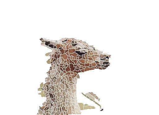
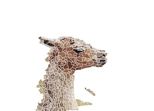
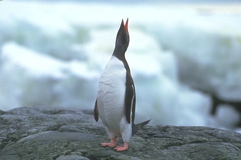
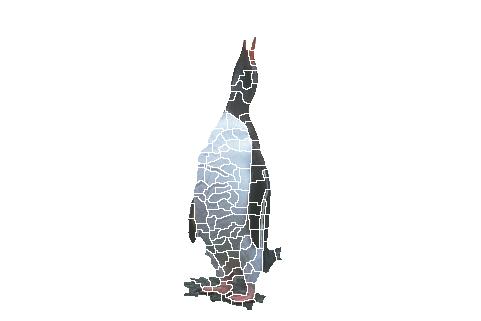
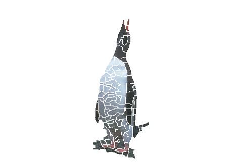
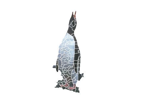
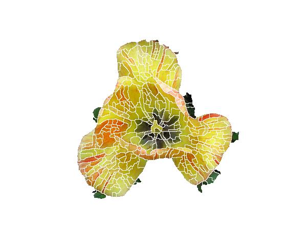
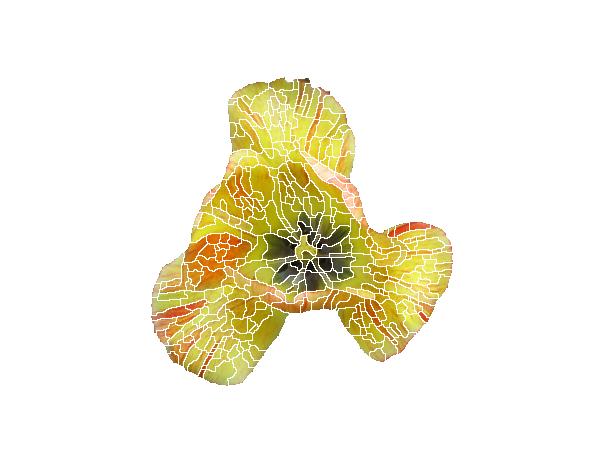
Figure 1: Segmentation results of the GrabCut dataset for a varying number of GMM components $K$. The left column depicts the input image.

The average segmentation accuracy with respect to $K$ is depicted in Fig. 2, for the proposed scheme and the GrabCut approach. It follows that the average accuracy is insensitive to the choice of $K$, and the mean accuracy of the proposed scheme is shown to outperform the GrabCut segmentation accuracy.

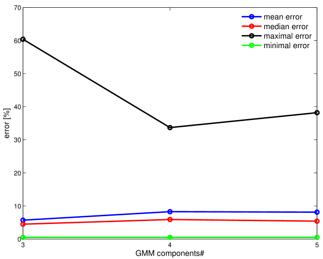
(a) Proposed scheme

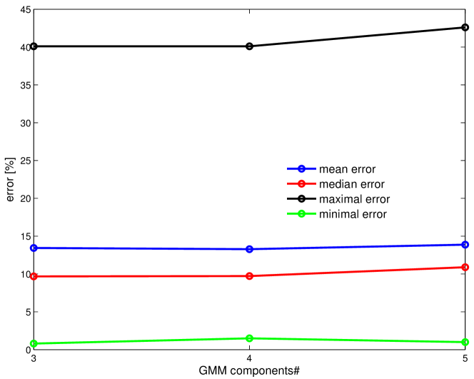
(b) GrabCut

Figure 2: Segmentation results of the GrabCut dataset for a varying number of GMM components $K=\left\{3,4,5\right\}$, for the proposed scheme (a) and GrabCut scheme (b).

We also studied the accuracy sensitivity with respect to $\lambda$, the relative weighting of the unary and binary terms, in Fig. 3. The average accuracy seems insensitive to the choice of $\lambda$, similar to the results in Fig. 2, where the proposed scheme outperforms the GrabCut. We note that due to the different potentials and weights used by the proposed scheme and GrabCut, respectively, we did not use the same values of $\lambda$ for both schemes. We varied $\lambda$ for both schemes around their default values.

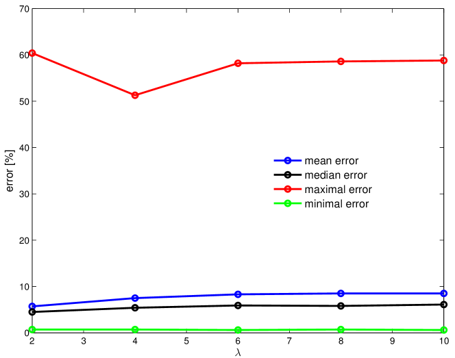
(a) Proposed scheme

(b) GrabCut

Figure 3: Segmentation accuracy of the GrabCut dataset using varying $\lambda$, the relative weighting of the unary and binary terms, for the proposed scheme (a) and GrabCut scheme (b).

Following Eq. 16, the larger $\lambda,$ the more relative weight is given to the unary probabilities that encode the $\mathcal{F}$/$\mathcal{B}$ color models. In contrast, the pairwise assignment probabilities encode the local classification structure. This is exemplified in Fig. 4 where we depict the visual outcome of varying $\lambda$. For $\lambda=2$ the pairwise probabilities dominate the segmentation, resulting in accurate boundaries, while as $\lambda$ increases the segmentation becomes less accurate.

$\lambda=2$	$\lambda=4$	$\lambda=6$	$\lambda=10$

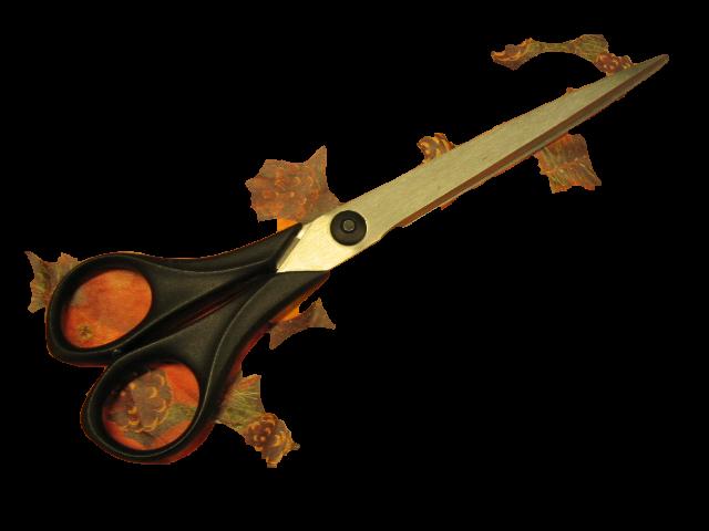
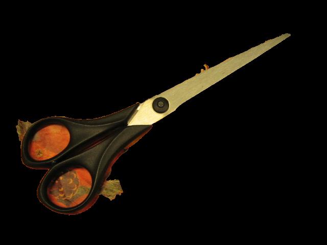
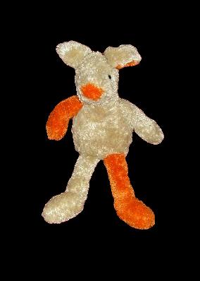
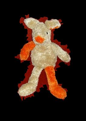
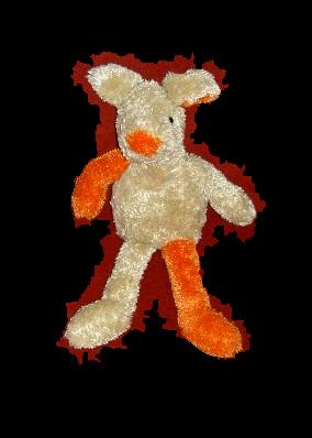
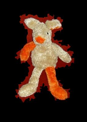
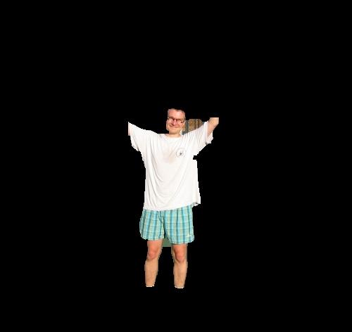
Figure 4: Segmentation results of the GrabCut dataset for varying weighting tradeoffs $\lambda$ between the unary and binary terms. The larger $\lambda$ the more emphasis is given to the unary term in Eq. 16.

In order to quantify the relative influence of the proposed inference scheme (Section III-C) and the proposed unary and pairwise terms (Sections III-C and III-A, respectively), on the segmentation accuracy, we reformulated the unary and pairwise terms as weights, and applied a state-of-the-art max-flow/min-cut solver . The unary and binary weights are given by

$$\phi\left(s_{i}\right)=1-p_{u}\left(s_{i}\in\mathcal{F}\right),$$ (21)

and

$$\phi\left(s_{i},s_{j}\right)={2\cdot}p\left(s_{i}\in\mathcal{F},s_{j}\in\mathcal{B}\right),$$ (22)

respectively, where $p_{u}\left(\cdot\right)$ and $p\left(\cdot,\cdot\right)$ are the unary and pairwise probabilities defined in Sections III-C and III-A. Figures 5a and 5b depict the results for a varying number of GMM components $K$ and relative weighting $\lambda$, respectively. It follows that using the proposed probabilities with the max-flow/min-cut solver results in lower segmentation accuracy.

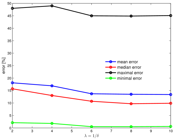
(a) Varying $\lambda$

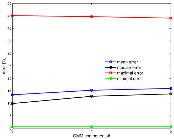
(b) Varying $K$

Figure 5: Image segmentation using the max-flow solver and the proposed probabilities as potentials. (a) Segmentation accuracy with respect to the relative weighting $\lambda$ using GMMs with $K=3$, and with respect to a varying number of GMM components in (b) .

We also applied the Loopy Belief Propagation (LBP) as a solver utilizing the unary and binary probabilities as in Fig. 5. For that we utilized the UGM toolbox, and the results are shown in Fig. 6. The LBP-based solver relates to the proposed scheme as both are probabilistic inference schemes, in contrast to the MaxFlow [3] that is a discrete optimization scheme. The main difference being that the PGM [10] is able to handle probabilities represented by dense graphs, while the LBP is optimal for trees and might diverge when applied to dense probabilistic graphs. The inference graph in image segmentation is typically sparse, as the pairwise probabilities only relate to neighboring SPs, thus allowing the LBP to converge. In our simulations depicted in Fig. 6, the LBP-based solver yielded an accuracy 7.3%, that is inferior to the proposed scheme.

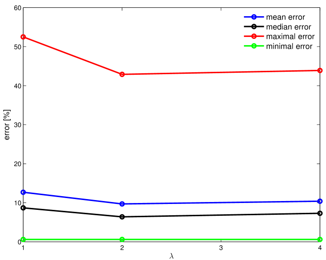
(a) Varying $\lambda$

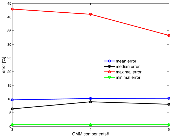
(b) Varying $K$

Figure 6: Image segmentation using the Loopy Belief Propagation solver and the proposed probabilities as potentials. (a) Segmentation accuracy with respect to the relative weighting $\lambda$ using GMMs with $K=3$.  (b) Segmentation accuracy with respect to the number of GMM components $K$ and $\lambda=2.$

We present additional qualitative segmentation results of the proposed scheme in Fig. 7

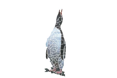
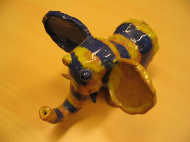
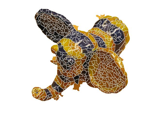
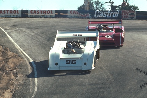
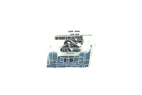
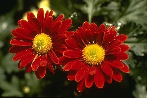
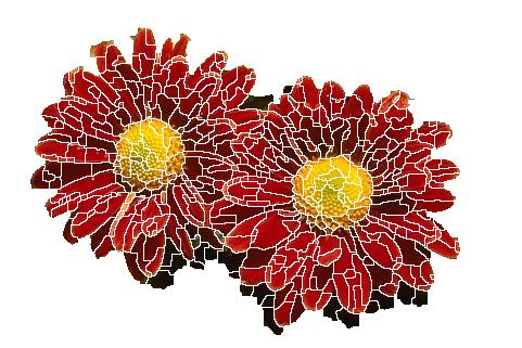
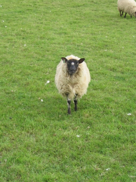
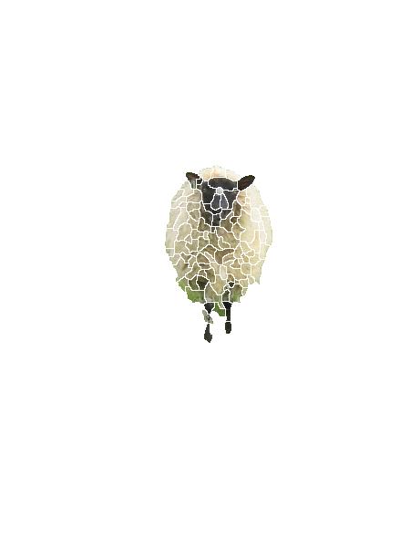
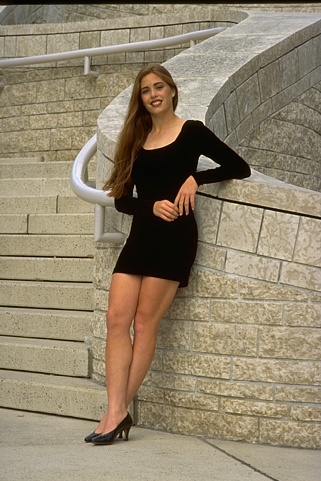
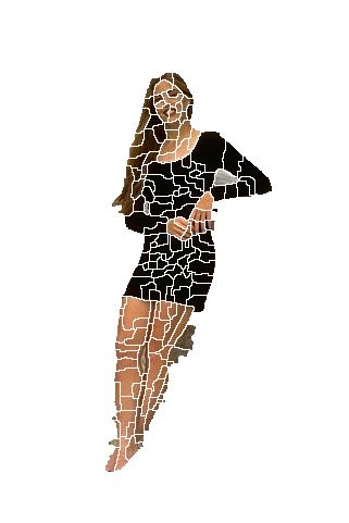
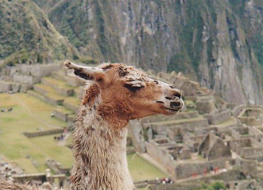
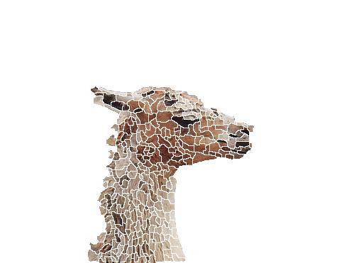
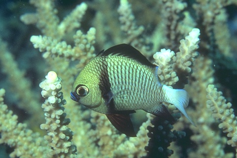
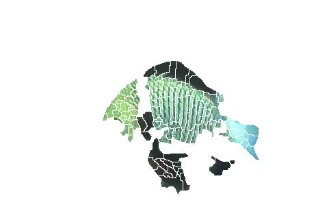
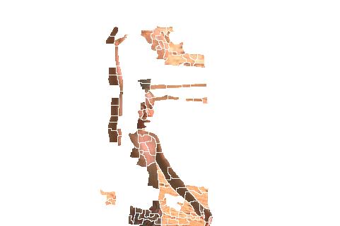
Figure 7: Segmentation results of the GrabCut dataset, using GMMs with $K=3$ components, and $N=3$ KNN for the pairwise assignment probabilities.

IV-B Pascal VOC Datasets

The Pascal VOC09 [11], Pascal VOC10 [12] and PASCAL VOC11 [13] datasets consist of 1499, 1928 and 2223 images, respectively. The PASCAL dataset groundtruth annotation consists of the annotations of 20 classes of objects, and we considered each annotated pixel as belonging to the foreground.

In this dataset the TriMap initialization set is not utilized, as in the GrabCut database, and is segmented in automatically. To add an initialization step, that provides a coarse estimate of the segmentation, we implemented the segmentation prior proposed by Rosenfeld et al. [32] and detailed in Section III-E, using $p_{0}=0.4$ as the background probability detection threshold. For each dataset, we randomly chose half of the images to train the detector. The background pixels closest to the unclassified portion of the image were used for background model training, similar to the user provided input in the semi-automatic formulation of our approach, and the proposed scheme was applied as in Section IV-A. We experimentally used $K=5$ GMM components for background modeling, and $K=3$ for foreground modeling, while the RBF bandwidths are auto-tuned using Eqs. 17 and 18.

We segment the image into $\mathcal{F}$/$\mathcal{B}$ regions, considering all the objects in the image as being foreground, and quantify the segmentation accuracy using the overlap score [32]

$$overlap=|\frac{S\cap S^{\prime}}{S\cup S^{\prime}}|$$ (23)

where $S$ is the ground truth and $S^{\prime}$ is the segmentation result.

Table II compares the mean overlap score for the segmentation of the Pascal VOC09, Pascal VOC10 and Pascal VOC11 datasets using the proposed scheme, CPMC [6] and the work of Kuettel et al. [20]. We also compare against Global Image Neighbor Transfer (GINT) and GrabCut 50% (GC50) that were used as a baseline by Kuettel et al. [20]. In GINT, the $m=5$ training images most similar to the test image, (according to the GIST descriptor) were averaged and thresholded to produce the final segmentation. In GC50, a patch consisting of 50% of the image size, located at the image center, was used as an initial estimate of the foreground.

We also compared against a variant of the proposed scheme, where the initial unary probabilities are estimated using only the background. The gist of this formulation is that the initial unknown region is known to consist of both $\mathcal{F}$ and $\mathcal{B}$ SPs, while the initial background region only consists of $\mathcal{B}$ SPs. The initial estimate of  the GMMs is thus given by

$$p_{u}\left(\mathbf{s}_{i}\in\mathcal{B}\right) =\exp\left(-\frac{\tilde{D}_{KL}(G_{i}\|GMM_{\mathcal{B}})}{\sigma_{u}}\right)\newline \newline ,$$ (24)

$$p_{u}\left(\mathbf{s}_{i}\in\mathcal{F}\right) =1-p_{u}\left(\mathbf{s}_{i}\in\mathcal{B}\right)$$ (25)

where $\sigma_{u}$ is estimated by

$$\sigma_{u}=\underset{G_{i}\in\mathcal{B}}{median}\tilde{D}_{KL}(G_{i}\|GMM_{\mathcal{B}}).$$ (26)

The remainder of the iterative refinement is applied as in Section III-D.

Method	VOC 2009	VOC 2010	VOC 2011
GC50[20]	-	0.30	-
GINT[20]	-	0.27	-
CPMC [6] (best K)	-	0.34	-
Kuettel et al [20]	-	0.48	-
Proposed scheme	0.46	0.47	0.47
Proposed scheme-gb	0.47	0.48	0.48

TABLE II: Segmentation results for the Pascal VOC09, VOC2010 and VOC11 datasets using the overlap score. The higher the overlap score, the better the segmentation accuracy.

Representative qualitative results are shown in Fig. 8.

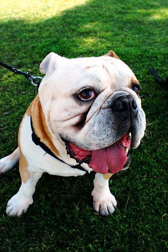
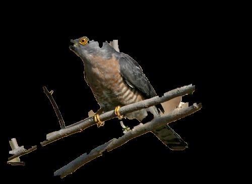
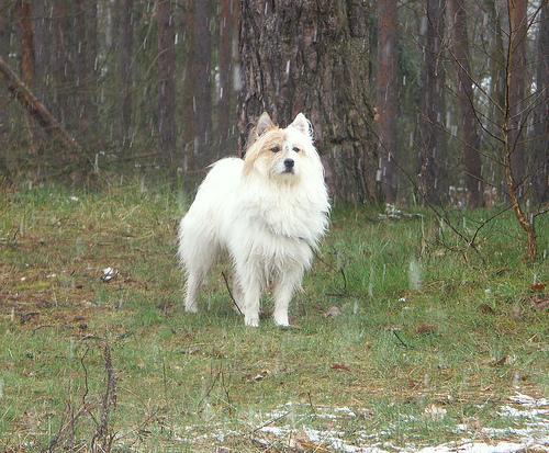
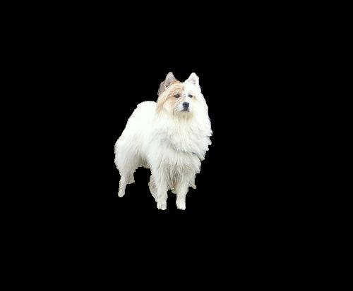
Figure 8: Representative segmentation results for the Pascal VOC 2011 dataset. We model both the foreground and the background as GMMs with $K=3$ components. The pairwise assignment probabilities utilize $m=3$ nearest neighbors, and the prior by Rosenfeld et al. [32] was used for initialization.

It follows that the proposed scheme compares favorably with contemporary state-of the-art schemes such as CPMC [6] all using the same initialization scheme, and performs similarly to Kuettel et al. [20], whose initialization scheme is more elaborated.

IV-C Runtime and Implementation

The proposed scheme was implemented in unoptimized Matlab code, and the simulations were ran on a Intel core i7 PC equipped with 8Gb of RAM. The runtime of the algorithm is 1-2 seconds per iteration, such that the runtime of 10 iterations is 15 seconds. As the distance matrix between the SPs is computed once (in the first iteration), most of the running time is spent computing the refined $\mathcal{F}$/$\mathcal{B}$ GMM models at each iteration. The spectral solver detailed in Section III-C requires $\sim 100ms$.

V Conclusions

In this work we presented an approach for Foreground/Backgrounds ($\mathcal{F}$/$\mathcal{B}$) image segmentation. Our scheme represents an image as a set of SPs, that are classified to either $\mathcal{F}$/$\mathcal{B}$. The classification is formulated using a probabilistic framework consisting of unary and pairwise probabilities estimated using low-level image features. SPs are statistically characterized by Gaussian models, allowing to define neighboring pairwise probabilities in terms of the KL distances between neighboring superpixels. The foreground and background are modeled via Gaussian mixture models, yielding a global representation of both, and estimate unary assignment probability by way of KL distances between the classes (GMMs) and the superpixels (Gaussians). The segmentation is thus formulated as an inference problem over a two-dimensional MRF. For that we applied a novel variation of a probabilistic inference scheme [10], which allows improved insights and an iterative auto-tuning scheme for the parameters of the unary and pairwise assignment probabilities. The proposed scheme is applied in both semi-supervised and unsupervised settings, and is shown to compare favorably with state-of-the-art schemes when applied to contemporary image testsets.

Ayelet Heimowitz received the BSc degree in Computer Engineering in 2009 from Bar Ilan University, Israel. She received the MSc degree in Electrical Engineering in 2011. She is currently studying toward the Ph.D. degree in Electrical Engineering in the Faculty of Engineering, Bar-Ilan University, Ramat-Gan, Israel.

Yosi Keller received the BSc degree in Electrical Engineering in 1994 from the Technion-Israel Institute of Technology, Haifa. He received the MSc and PhD degrees in electrical engineering from Tel-Aviv University, Tel-Aviv, in 1998 and 2003, respectively. From 2003 to 2006 he was a Gibbs assistant professor with the Department of Mathematics, Yale University. He is an Associate Professor at the Faculty of Engineering in Bar Ilan University, Israel.

References

- [1] S. Alpert, M. Galun, A. Brandt, and R. Basri. Image segmentation by probabilistic bottom-up aggregation and cue integration. IEEE Transactions on Pattern Analysis and Machine Intelligence (PAMI), 34(2):315–327, 2012.
- [2] Y. Boykov and V. Kolmogorov. Computing geodesics and minimal surfaces via graph cuts. In Proceedings of the International Conference on Computer Vision (ICCV), pages 26–33 vol.1, October 2003.
- [3] Y. Boykov and V. Kolmogorov. Computing geodesics and minimal surfaces via graph cuts. In Proceedings of the International Conference on Computer Vision (ICCV), pages 26–33 vol.1, October 2003.
- [4] Yuri Boykov, Olga Veksler, and Ramin Zabih. Fast approximate energy minimization via graph cuts. IEEE Transactions on Pattern Analysis and Machine Intelligence (PAMI), 23(11):1222–1239, November 2001.
- [5] Y.Y. Boykov and M.-P. Jolly. Interactive graph cuts for optimal boundary amp; region segmentation of objects in n-d images. In Proceedings of the International Conference on Computer Vision (ICCV), volume 1, pages 105–112 vol.1, 2001.
- [6] J. Carreira and C. Sminchisescu. Constrained parametric min-cuts for automatic object segmentation. In Proceedings of the IEEE Conference on Computer Vision and Pattern Recognition (CVPR), pages 3241–3248, June 2010.
- [7] Joao Carreira and Cristian Sminchisescu. CPMC: Automatic object segmentation using constrained parametric min-cuts. IEEE Transactions on Pattern Analysis and Machine Intelligence (PAMI), 34(7):1312–1328, 2012.
- [8] Chao Chen, D. Freedman, and Christoph H. Lampert. Enforcing topological constraints in random field image segmentation. In Proceedings of the IEEE Conference on Computer Vision and Pattern Recognition (CVPR), pages 2089–2096, June 2011.
- [9] P. Das and O. Veksler. Semiautomatic segmentation with compact shapre prior. In Computer and Robot Vision, 2006. The 3rd Canadian Conference on, page 28, June 2006.
- [10] A. Egozi, Y. Keller, and H. Guterman. A probabilistic approach to spectral graph matching. IEEE Transactions on Pattern Analysis and Machine Intelligence (PAMI), 35(1):18–27, January 2013.
- [11] M. Everingham, L. Van Gool, C. K. I. Williams, J. Winn, and A. Zisserman. The PASCAL Visual Object Classes Challenge 2009 (VOC2009) Results. http://www.pascal-network.org/challenges/VOC/voc2009/workshop/index.html.
- [12] M. Everingham, L. Van Gool, C. K. I. Williams, J. Winn, and A. Zisserman. The PASCAL Visual Object Classes Challenge 2010 (VOC2010) Results. http://www.pascal-network.org/challenges/VOC/voc2010/workshop/index.html.
- [13] M. Everingham, L. Van Gool, C. K. I. Williams, J. Winn, and A. Zisserman. The PASCAL Visual Object Classes Challenge 2011 (VOC2011) Results. http://www.pascal-network.org/challenges/VOC/voc2011/workshop/index.html.
- [14] D. Freedman and Tao Zhang. Interactive graph cut based segmentation with shape priors. In Proceedings of the IEEE Conference on Computer Vision and Pattern Recognition (CVPR), volume 1, pages 755–762, June 2005.
- [15] R. Girshick, J. Donahue, T. Darrell, and J. Malik. Rich feature hierarchies for accurate object detection and semantic segmentation. In Proceedings of the IEEE Conference on Computer Vision and Pattern Recognition (CVPR), pages 580–587, Los Alamitos, CA, USA, June 2014. IEEE Computer Society.
- [16] J. Goldberger, S. Gordon, and H. Greenspan. An efficient image similarity measure based on approximations of kl-divergence between two gaussian mixtures. In Proceedings of the International Conference on Computer Vision (ICCV), pages 487–493 vol.1, October 2003.
- [17] Bharath Hariharan, Pablo Arbeláez, Ross Girshick, and Jitendra Malik. Simultaneous detection and segmentation. In Proceedings of the European Conference on Computer Vision (ECCV), 2014.
- [18] S. Jianbo and J. Malik. Normalized cuts and image segmentation. IEEE Transactions on Pattern Analysis and Machine Intelligence (PAMI), 22(8):888 –905, August 2000.
- [19] Philipp Krähenbühl and Vladlen Koltun. Efficient inference in fully connected crfs with gaussian edge potentials. In J. Shawe-Taylor, R.S. Zemel, P.L. Bartlett, F. Pereira, and K.Q. Weinberger, editors, Neural Information Processing Systems (NeurIPS), pages 109–117. Curran Associates, Inc., 2011.
- [20] D. Kuettel and V. Ferrari. Figure-ground segmentation by transferring window masks. In Proceedings of the IEEE Conference on Computer Vision and Pattern Recognition (CVPR), pages 558–565, June 2012.
- [21] V. Lempitsky, P. Kohli, C. Rother, and T. Sharp. Image segmentation with a bounding box prior. In Proceedings of the International Conference on Computer Vision (ICCV), pages 277–284, September 2009.
- [22] M. Leordeanu and M. Hebert. A spectral technique for correspondence problems using pairwise constraints. In Proceedings of the International Conference on Computer Vision (ICCV), volume 2, pages 1482 – 1489, October 2005.
- [23] A. Levinshtein, A. Stere, K.N. Kutulakos, D.J. Fleet, S.J. Dickinson, and K. Siddiqi. TurboPixels: Fast superpixels using geometric flows. IEEE Transactions on Pattern Analysis and Machine Intelligence (PAMI), 31(12):2290–2297, December 2009.
- [24] Yin Li, Jian Sun, Chi-Keung Tang, and Heung-Yeung Shum. Lazy snapping. ACM Trans. Graph., 23(3):303–308, August 2004.
- [25] H. Lombaert, Yiyong Sun, L. Grady, and Chenyang Xu. A multilevel banded graph cuts method for fast image segmentation. In Proceedings of the International Conference on Computer Vision (ICCV), volume 1, pages 259–265 Vol. 1, October 2005.
- [26] Jonathan Long, Evan Shelhamer, and Trevor Darrell. Fully convolutional networks for semantic segmentation. Proceedings of the IEEE Conference on Computer Vision and Pattern Recognition (CVPR), November 2015.
- [27] G. J. McLachlan and D. Peel. Finite mixture models. Wiley Series in Probability and Statistics, New York, 2000.
- [28] Andrew Y. Ng, Michael I. Jordan, and Yair Weiss. On spectral clustering: Analysis and an algorithm. In T.G. Dietterich, S. Becker, and Z. Ghahramani, editors, Neural Information Processing Systems (NeurIPS), pages 849–856. MIT Press, 2002.
- [29] Aude Oliva and Antonio Torralba. Modeling the shape of the scene: A holistic representation of the spatial envelope. International Journal of Computer Vision (IJCV), 42(3):145–175, May 2001.
- [30] Ana Oliveira-Brochado and Francisco Vitorino Martins. Assessing the Number of Components in Mixture Models: a Review. FEP Working Papers 194, Universidade do Porto, Faculdade de Economia do Porto, November 2005.
- [31] Shaoqing Ren, Kaiming He, Ross Girshick, and Jian Sun. Faster R-CNN: Towards real-time object detection with region proposal networks. In Neural Information Processing Systems (NeurIPS), 2015.
- [32] A. Rosenfeld and D. Weinshall. Extracting foreground masks towards object recognition. In Proceedings of the International Conference on Computer Vision (ICCV), pages 1371 –1378, nov. 2011.
- [33] Carsten Rother, Vladimir Kolmogorov, and Andrew Blake. ”grabcut”: Interactive foreground extraction using iterated graph cuts. ACM Trans. Graph., 23(3):309–314, August 2004.
- [34] A. Septimus, Y. Keller, and I. Bergel. A spectral approach to inter-carrier interference mitigation in ofdm systems. Communications, IEEE Transactions on, 62(8):2802–2811, August 2014.
- [35] Jianbo Shi and Jitendra Malik. Normalized cuts and image segmentation. IEEE Transactions on Pattern Analysis and Machine Intelligence (PAMI), 22(8):888–905, August 2000.
- [36] G. Slabaugh and G. Unal. Graph cuts segmentation using an elliptical shape prior. In Proceedings of the IEEE International Conference on Image Processing (ICIP), volume 2, pages II–1222, 2005.
- [37] K.E.A. van de Sande, T. Gevers, and C.G.M. Snoek. Evaluating color descriptors for object and scene recognition. IEEE Transactions on Pattern Analysis and Machine Intelligence (PAMI), 32(9):1582–1596, September 2010.
- [38] Olga Veksler. Star shape prior for graph-cut image segmentation. In Proceedings of the 10th European Conference on Computer Vision: Part III, Proceedings of the European Conference on Computer Vision (ECCV), pages 454–467, Berlin, Heidelberg, 2008. Springer-Verlag.
- [39] L. Vincent and P. Soille. Watersheds in digital spaces: An efficient algorithm based on immersion simulations. IEEE Transactions on Pattern Analysis and Machine Intelligence (PAMI), 13:583–598, 1991.
- [40] Y. Weiss and W. T. Freeman. On the optimality of solutions of the max-product belief-propagation algorithm in arbitrary graphs. IEEE Transactions on Information Theory, 47(2):736–744, September 2001.
- [41] Ming Xiumingzhang. GrabCut Matlab implmentation. https://github.com/xiumingzhang/grabcut.
- [42] Linli Xu, Wenye Li, and D. Schuurmans. Fast normalized cut with linear constraints. In Proceedings of the IEEE Conference on Computer Vision and Pattern Recognition (CVPR), pages 2866–2873, June 2009.
- [43] Qingxiong Yang, Liang Wang, and N. Ahuja. A constant-space belief propagation algorithm for stereo matching. In Proceedings of the IEEE Conference on Computer Vision and Pattern Recognition (CVPR), pages 1458–1465, June 2010.
- [44] S.X. Yu and Jianbo Shi. Segmentation given partial grouping constraints. IEEE Transactions on Pattern Analysis and Machine Intelligence (PAMI), 26(2):173–183, Feb 2004.
- [45] S. Zheng, S. Jayasumana, B. Romera-Paredes, V. Vineet, Z. Su, D. Du, C. Huang, and P.H.S. Torr. Conditional Random Fields as Recurrent Neural Networks. In Proceedings of the International Conference on Computer Vision (ICCV), 2015.