APNet: An All-Frame-Level Neural Vocoder Incorporating Direct Prediction of Amplitude and Phase Spectra

Abstract

This paper presents a novel neural vocoder named APNet which reconstructs speech waveforms from acoustic features by predicting amplitude and phase spectra directly. The APNet vocoder is composed of an amplitude spectrum predictor (ASP) and a phase spectrum predictor (PSP). The ASP is a residual convolution network which predicts frame-level log amplitude spectra from acoustic features. The PSP also adopts a residual convolution network using acoustic features as input, then passes the output of this network through two parallel linear convolution layers respectively, and finally integrates into a phase calculation formula to estimate frame-level phase spectra. Finally, the outputs of ASP and PSP are combined to reconstruct speech waveforms by inverse short-time Fourier transform (ISTFT). All operations of the ASP and PSP are performed at the frame level. We train the ASP and PSP jointly and define multilevel loss functions based on amplitude mean square error, phase anti-wrapping error, short-time spectral inconsistency error and time domain reconstruction error. Experimental results show that our proposed APNet vocoder achieves an approximately 8x faster inference speed than HiFi-GAN v1 on a CPU due to the all-frame-level operations, while its synthesized speech quality is comparable to HiFi-GAN v1. The synthesized speech quality of the APNet vocoder is also better than that of several equally efficient models. Ablation experiments also confirm that the proposed parallel phase estimation architecture is essential to phase modeling and the proposed loss functions are helpful for improving the synthesized speech quality.

I Introduction

Speech synthesis, also known as text-to-speech (TTS), converts any input text into natural and fluent speech and solves the problem of how to make machines speak like humans. A speech synthesis system with high naturalness, intelligibility and expressiveness is a goal pursued by speech synthesis researchers. In recent years, statistical parametric speech synthesis (SPSS) [1] has become the mainstream speech synthesis method. It has the advantages of small system size, high robustness and flexibility. The acoustic model and vocoder are two key modules in the SPSS framework. The acoustic model describes the mapping relationship from text to acoustic features and currently incorporates many advanced structures, such as Tacotron [2], Tacotron2 [3], and Transformer [4], which outperform the conventional hidden Markov model (HMM) [5], deep neural network (DNN) [6] and recurrent neural network (RNN) [7] based methods. Vocoders [8], which reconstruct speech waveforms from acoustic features (e.g., mel spectrograms), also play an important role in SPSS. Their performance significantly affects the quality of synthetic speech. Some conventional vocoders (e.g., STRAIGHT [9] and WORLD [10]) have some deficiencies, such as the loss of spectral details and phase information. Thanks to the development of deep learning and neural networks, neural vocoders have emerged and gradually replaced the conventional ones. Neural vocoders can also be applied to other tasks, such as voice conversion [11], bandwidth extension [12] and speech enhancement [13].

The synthesized speech quality and inference efficiency are the two main considerations for evaluating neural vocoders. Initially, autoregressive neural waveform generation models represented by WaveNet [14], SampleRNN [15] and WaveRNN [16] were proposed and successfully applied in the construction of neural vocoders [17, 18, 19, 20, 21, 22]. Although autoregressive neural vocoders achieved breakthroughs in synthesized speech quality compared to conventional ones, their inference efficiency was unsatisfactory due to the autoregressive inference mode of raw waveforms with a high sampling rate. Subsequently, knowledge-distilling-based models (e.g., Parallel WaveNet [23] and ClariNet [24]), flow-based models (e.g., WaveGlow [25] and WaveFlow [26]), and glottis-based models (e.g., GlotNet [27] and LPCNet [28]) were proposed. Although the inference efficiency of these models has improved significantly, the overall computational complexity was still high, limiting their use in resource-constrained environments such as embedded devices. Recently, waveform generation models without autoregressive and flow-like structures have received more attention. The neural source-filter (NSF) model [29] combined speech production mechanisms with neural networks and achieved the prediction of speech waveforms from explicit F0 and mel spectrograms. Generative adversarial network (GAN) [30] based models, such as WaveGAN [31], GAN-TTS [32], MelGAN [33], Parallel WaveGAN [34] and HiFi-GAN [35], leveraged GANs to ensure the synthesized speech quality and improved the efficiency by parallelizable training and inference through noncausal convolutions. For example, HiFi-GAN [35] cascades multiple upsampling layers and residual convolution networks to gradually upsample the input mel spectrogram to the sampling rate of the final waveform while performing convolution operations. It also adopts adversarial training to ensure high-fidelity waveform generation. However, these GAN-based models always directly predict the final waveforms, so the problem of slow inference still exists.

A speech waveform can be interconverted with its amplitude and phase spectra. Predicting the amplitude and phase spectra instead of the waveform from the input acoustic features is a new approach to build neural vocoders. To improve the inference efficiency of HiFi-GAN, ISTFTNET [36] proposes to output the amplitude and phase spectra close to the waveform sampling rate in the middle layer of HiFi-GAN and then synthesize the final waveform through inverse short-time Fourier transform (ISTFT). However, the results reported in ISTFTNET [36] show that predicting amplitude and phase spectra at low sampling rates is difficult. In our previous work, we proposed a neural vocoder named HiNet [37] which reconstructs speech waveforms from acoustic features by predicting amplitude and phase spectra hierarchically. The predicted spectra are at the same sampling rate as the acoustic features. Unfortunately, limited by the issue of phase wrapping and the difficulty of phase modeling, the HiNet vocoder still needs an NSF-like model to generate an intermediate waveform for further phase extraction through short-time Fourier transform (STFT). To our knowledge, synthesizing a waveform by predicting its raw amplitude and phase spectra directly has not yet been thoroughly investigated.

Therefore, this paper proposes a novel neural vocoder named APNet, which incorporates the direct prediction of amplitude and phase spectra. Similar to the HiNet vocoder, the proposed APNet vocoder consists of an amplitude spectrum predictor (ASP) and a phase spectrum predictor (PSP). The ASP and PSP predict the raw amplitude and phase spectra at the same sampling rate as the acoustic features, respectively, and then the final waveform is synthesized through ISTFT. Compared to the HiNet vocoder, the APNet vocoder 1) jointly trains the ASP and PSP and 2) predicts the phase spectra directly. The ASP is a residual convolution network which predicts frame-level log amplitude spectra from acoustic features. The PSP also adopts a residual convolution network using acoustic features as input. Then, the output of the network is passed through two parallel linear convolution layers respectively to obtain two outputs, and then the frame-level phase spectra are estimated by a phase calculation formula. Therefore, all operations in APNet are performed at the frame level, expecting to significantly improve the inference efficiency. We also propose multilevel loss functions defined on predicted log amplitude spectra, phase spectra, reconstructed STFT spectra and final waveforms to ensure the fidelity of the amplitude spectra, the precision of the phase spectra, the consistency of the STFT spectra and the quality of the final waveforms. Experimental results show that the synthesized speech quality of our proposed APNet vocoder is comparable to that of HiFi-GAN v1 [35], but its inference efficiency is significantly improved due to the all-frame-level operations, reaching 14x real-time on a CPU, which is 8x faster than HiFi-GAN v1. Although the inference efficiency on a CPU of multi-band MelGAN [38] and ISTFTNET [36] is similar to our model, their synthesized speech quality is clearly inferior to our model. The APNet vocoder outperforms the HiNet vocoder in terms of both synthesized speech quality and inference efficiency. We also conduct several ablation experiments to explore the roles of specific structures and loss functions. Interestingly, the proposed parallel phase estimation architecture is the key to successful phase modeling. The proposed loss functions also help to improve the synthesized speech quality.

There are two main contributions of the APNet vocoder. First, the APNet achieves all-frame-level speech waveform generation, which greatly improves the inference efficiency by predicting the frame-level amplitude and phase spectra. Second, the proposed parallel phase estimation architecture in APNet successfully achieves phase modeling using neural networks, which provides a new idea for the tricky phase estimation task.

This paper is organized as follows: In Section II, we briefly review the HiFi-GAN [35], ISTFTNET [36] and our previously proposed HiNet vocoder [37], respectively. In Section III, we provide details on our proposed APNet vocoder. In Section IV, we present our experimental results. Finally, we give conclusions in Section V.

II Related Works

In this section, we briefly introduce the HiFi-GAN [35], ISTFTNET [36] and HiNet vocoders [37], respectively. These vocoders are used for comparison with our proposed APNet vocoder in the experiments. Figure 1 shows a model structure comparison among the four vocoders.

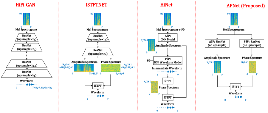
Figure 1: Model structure comparison among the HiFi-GAN, ISTFTNET, HiNet and APNet vocoders. Here, ASP and PSP represent the amplitude spectrum predictor and phase spectrum predictor, respectively. ResNet, CNN and NSF represent the residual convolution network, convolutional neural network and neural source-filter, respectively. STFT and ISTFT represent the short-time Fourier transform and inverse short-time Fourier transform, respectively.

II-A HiFi-GAN

As shown in Figure 1, HiFi-GAN [35] cascades $B$ residual convolution networks, converting 80-dimensional frame-level mel spectrogram $\bm{M}\in\mathbb{R}^{F\times 80}$ with length $F$ to waveform $\hat{\bm{x}}\in\mathbb{R}^{T}$ with length $T$. $\frac{T}{F}$ is also equal to the frame shift when extracting the mel spectrogram from a waveform. The residual convolution network includes dilated convolution, residual connections, skip connections, etc. There is an upsampling layer in front of each convolutional network, gradually raising the length $F$ of $\bm{M}$ to the length $T$ of $\hat{\bm{x}}$. Suppose the upsampling ratio of the $b$-th residual convolution network is $h_{b}$, where $b=1,2,\dots,B$, then we can obtain $T=H_{B}\cdot F$, where $H_{b}=h_{1}\cdot h_{2}\cdots h_{b},b=1,\dots,B$. Assume that the sampling rate of the waveform is $f_{s}$. Obviously, HiFi-GAN operates at multiple sampling rates, which are $F\cdot\frac{f_{s}}{T},H_{1}F\cdot\frac{f_{s}}{T},\dots,H_{B-1}F\cdot\frac{f_{s}}{T},f_{s}$. HiFi-GAN adopts adversarial training with multi-period discriminator (MPD) and multi-scale discriminator (MSD) to ensure high-fidelity waveform generation. The final loss of HiFi-GAN is a combination of GAN loss, feature matching loss and mel spectrogram loss.

II-B ISTFTNET

To improve the inference efficiency, ISTFTNET [36] incorporates ISTFT into HiFi-GAN. As shown in Figure 1, ISTFTNET outputs the amplitude spectrum $\hat{\bm{A}}\in\mathbb{R}^{T_{b}\times(N_{b}/2+1)}$ and phase spectrum $\hat{\bm{P}}\in\mathbb{R}^{T_{b}\times(N_{b}/2+1)}$ with sampling rate $H_{b}F\cdot\frac{f_{s}}{T}$ after the intermediate $b$-th ($1<b<B$) residual convolution network of HiFi-GAN and then synthesizes the final waveform through ISTFT. Although the predicted amplitude and phase spectra are of length $T_{b}=H_{b}\cdot F>F$, their FFT point number is $N_{b}=\frac{N}{H_{b}}<N$, where $N$ is the FFT point number when extracting the mel spectrogram from a waveform. That is, ISTFTNET predicts amplitude and phase spectra with high time resolution and low frequency resolution. Therefore, ISTFTNET operates at multiple sampling rates, which are $F\cdot\frac{f_{s}}{T},H_{1}F\cdot\frac{f_{s}}{T},\dots,H_{b}F\cdot\frac{f_{s}}{T}$, and hence achieves higher inference efficiency than HiFi-GAN. However, the results reported in ISTFTNET [36] show that predicting amplitude and phase spectra at low sampling rates is tricky, i.e., $T_{b}$ cannot be too small than $T$.

II-C HiNet

In our previous work, we proposed the HiNet vocoder [37] and its variant [39]. We have also successfully applied the HiNet vocoder in the reverberation modeling task [40] and denoising and dereveberation task [41, 42], respectively. As shown in Figure 1, the HiNet vocoder uses an ASP and a PSP to predict the frame-level log amplitude spectrum and phase spectrum of a waveform, respectively. During the inference process, the ASP predicts the log amplitude spectrum $\log\hat{\bm{A}}\in\mathbb{R}^{F\times(N/2+1)}$ from the input mel spectrogram and F0, and the PSP predicts the phase spectrum $\hat{\bm{P}}\in\mathbb{R}^{F\times(N/2+1)}$ from the input F0 and predicted log amplitude spectrum by ASP. The length and FFT point number of $\hat{\bm{A}}$ and $\hat{\bm{P}}$ are $F$ and $N$ respectively, which are the same as those of the input mel spectrogram. It then reconstructs the waveform from the predicted amplitude and phase spectra through ISTFT. The ASP is a frame-level convolutional neural network (CNN) containing multiple convolutional layers. However, limited by the difficulty of phase modeling, the PSP is constructed by concatenating a lightweight NSF-like neural waveform model with a phase spectrum extractor. The NSF-like model predicts an intermediate waveform $\hat{\bm{x}}_{I}\in\mathbb{R}^{T}$ and then the extractor extracts the phase spectrum from $\hat{\bm{x}}_{I}$ through STFT. HiNet operates at two sampling rates which are $F\cdot\frac{f_{s}}{T}$ and $f_{s}$, and still fails to achieve all-frame-level waveform generation at the unique raw sampling rate $F\cdot\frac{f_{s}}{T}$.

III Proposed Methods

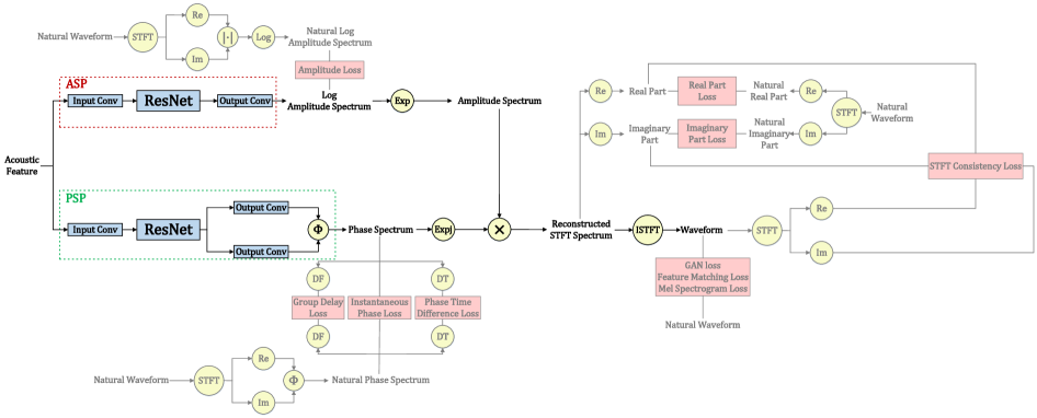
Figure 2: Details of the APNet vocoder. Here, ASP and PSP represent the amplitude spectrum predictor and phase spectrum predictor, respectively. Blue boxes, red boxes and yellow circles represent trainable modules, loss functions and basic operations, respectively. ResBlock and Conv represent the residual convolution network and linear convolution layer, respectively. STFT, ISTFT, Re, Im, $|\cdot|$, $\Phi$, DF, DT, Exp, Log, Expj and $\times$ represent the short-time Fourier transform, inverse short-time Fourier transform, real part calculation, imaginary part calculation, amplitude calculation, phase calculation, differential along frequency axis, differential along time axis, natural exponential function, logarithm, complex exponential function $e^{j\cdot}$ and element-wise multiplication, respectively. GAN denotes generative adversarial network. Gray parts do not appear during inference.

As shown in Figure 1, the proposed APNet vocoder directly predicts the speech amplitude spectrum $\hat{\bm{A}}\in\mathbb{R}^{F\times(N/2+1)}$ and phase spectrum $\hat{\bm{P}}\in\mathbb{R}^{F\times(N/2+1)}$ at unique raw sampling rate $F\cdot\frac{f_{s}}{T}$ from input acoustic feature (e.g., mel spectrogram $\bm{M}\in\mathbb{R}^{F\times 80}$). Then, the amplitude and phase spectra are reconstructed to the STFT spectrum $\hat{\bm{S}}\in\mathbb{C}^{F\times(N/2+1)}$, and finally, a waveform $\hat{\bm{x}}\in\mathbb{R}^{T}$ is recovered through ISTFT. The whole process can be described by the following mathematical expression:

$$\log\hat{\bm{A}}=ASP(\bm{M}),$$ (1)

$$\hat{\bm{P}}=PSP(\bm{M}),$$ (2)

$$\hat{\bm{S}}=\hat{\bm{A}}\cdot e^{j\hat{\bm{P}}},$$ (3)

$$\hat{\bm{x}}=ISTFT(\hat{\bm{S}}).$$ (4)

Therefore, the APNet vocoder is an all-frame-level model and only operates at sampling rate $F\cdot\frac{f_{s}}{T}$. Detailed structure and loss functions are shown in Figure 2. In Figure 2, only the blue boxes are trainable, and the gray part disappears during the inference process.

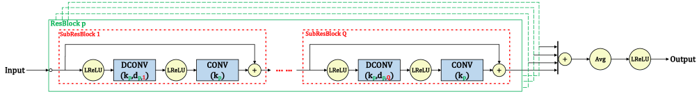
Figure 3: Details of the residual convolution network used in the ASP and PSP. Here, CONV, DCONV, ResBlock and SubResBlock represent the linear convolution layer, linear dilated convolution layer, residual convolution block and residual convolution subblock, respectively. LReLU, Avg and $+$ represent leaky rectified linear unit, average and addition, respectively. $k_{*}$ and $d_{*,*}$ denotes kernel size and dilation factor, respectively.

III-A Amplitude Spectrum Predictor

As shown in Figure 2, the ASP predicts the log amplitude spectrum $\log\hat{\bm{A}}$ from input acoustic feature (i.e., Equation 1). It consists of an input linear convolution layer, a residual convolution network and an output linear convolution layer. The details of the residual convolution network are shown in Figure 3. The residual convolution network consists of $P$ parallel residual convolution blocks (i.e., ResBlock in Figure 3), all of which have the same input. Then, the outputs of these $P$ blocks are summed (i.e., skip connections), averaged (i.e., divided by $P$), and finally activated by a leaky rectified linear unit (LReLU) [43]. The $p$-th block ($p=1,\dots,P$) is formed by concatenating $Q$ residual convolution subblocks (i.e., SubResBlock in Figure 3). In the $q$-th subblock ($q=1,\dots,Q$) of the $p$-th block ($p=1,\dots,P$), the input is first activated by LReLU, then passes through a linear dilated convolution layer (kernel size $=k_{p}$ and dilation factor $=d_{p,q}$), then is activated by LReLU again, passes through a normal linear convolution layer (kernel size $=k_{p}$), and finally superimposes with the input (i.e., residual connections) to obtain the output.

III-B Phase Spectrum Predictor

As shown in Figure 2, the PSP predicts the phase spectrum $\hat{\bm{P}}$ from input acoustic feature (i.e., Equation 2). It consists of an input linear convolution layer, a residual convolution network, two parallel output linear convolution layers and a phase calculation formula $\bm{\Phi}$. The residual convolution network is exactly the same as the one used in ASP. Assuming that two parallel output layers output $\bm{\widetilde{R}}$ and $\bm{\widetilde{I}}$ respectively, then

$$\hat{\bm{P}}=\bm{\Phi}(\bm{\widetilde{R}},\bm{\widetilde{I}}).$$ (5)

Note that Equation 5 is calculated element-wise, i.e., $\hat{P}_{f,n}=\bm{\Phi}(\widetilde{R}_{f,n},\widetilde{I}_{f,n}$), $f=1,\dots,F,n=1,\dots,\frac{N}{2}+1$, where $\hat{P}_{f,n}$, $\widetilde{R}_{f,n}$ and $\widetilde{I}_{f,n}$ are the elements in $\hat{\bm{P}}$, $\bm{\widetilde{R}}$ and $\bm{\widetilde{I}}$, respectively. The range of values for the phase is $-\pi<\hat{P}_{f,n}\leq\pi$.

We derive the mathematical expression for phase calculation formula $\bm{\Phi}$. First, we define two real numbers $R\in\mathbb{R}$ and $I\in\mathbb{R}$, and define a new symbolic function

$$Sgn^{*}(x)=\left\{\begin{array}[]{rl}1,&x\geq 0\\ -1,&x<0\end{array}\right..$$ (8)

The phase calculation formula $\bm{\Phi}$ is a function with two variables. Since $\arctan(-\infty)=-\frac{\pi}{2}$ and $\arctan(+\infty)=\frac{\pi}{2}$, $\bm{\Phi}(R,I)$ can be written by arctangent and symbolic functions as follows

$$\bm{\Phi}(R,I)=\arctan\left(\dfrac{I}{R}\right)-\dfrac{\pi}{2}\cdot Sgn^{*}(I)\cdot\left[Sgn^{*}(R)-1\right],$$ (9)

and sets $\bm{\Phi}(0,0)=0$. For $\forall R\in\mathbb{R}$ and $I\in\mathbb{R}$, $-\pi<\bm{\Phi}(R,I)\leq\pi$ (i.e., the resulting phase value is restricted within the principal value interval $(-\pi,\pi]$). To visually explain Equation 9, we draw a quadrant diagram shown in Figure 4. The horizontal and vertical axes represent $R$ and $I$, respectively. Figure 4 reveals the value range of $\bm{\Phi}(R,I)$ when $R$ and $I$ take different values. When the vector $(R,I)$ is located at the origin or on the real horizontal axis, $\bm{\Phi}(R,I)=0$; when the vector $(R,I)$ is in the first and second quadrants (including the positive vertical axis and negative horizontal axis), $\bm{\Phi}(R,I)$ is the angle through which the vector $(1,0)$ rotates counterclockwise to the vector $(R,I)$; when the vector $(R,I)$ is in the third and fourth quadrants (including the negative vertical axis), $\bm{\Phi}(R,I)$ is the negative angle through which the vector $(1,0)$ rotates clockwise to the vector $(R,I)$.

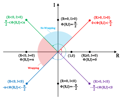
Figure 4: A quadrant diagram used to explain the phase calculation formula $\bm{\Phi}(R,I)$ and the phase wrapping issue.

We name these two parallel output layers and the phase calculation formula $\bm{\Phi}$ as parallel phase estimation architecture. The proposed architecture is the key to successful phase modeling, which is confirmed in the following experiments.

III-C Training and Inference Process

At the training stage, we jointly train the ASP and PSP and define multilevel loss functions on predicted log amplitude spectra, phase spectra, reconstructed STFT spectra and final waveforms as shown in the red boxes in Figure 2. These loss functions are expected to ensure the fidelity of the amplitude spectra, the precision of the phase spectra, the consistency of the STFT spectra and the quality of the final waveforms. These loss functions are described below.

III-C1 Losses defined on log amplitude spectra

The losses defined on log amplitude spectra are used to close the gap between the predicted log amplitude spectra and the natural ones, facilitating the generation of high-quality and high-fidelity log amplitude spectra, including:

• Amplitude Loss: The amplitude loss is the mean square error (MSE) between the predicted log amplitude spectrum $\log\hat{\bm{A}}$ and the natural one $\log\bm{A}$, i.e.,

  $$\mathcal{L}_{A}=\mathbb{E}_{\left(\log\hat{\bm{A}},\log\bm{A}\right)}\overline{\left(\log\hat{\bm{A}}-\log\bm{A}\right)^{2}},$$ (10)

  where $\overline{\bm{X}}$ means averaging all elements in the matrix $\bm{X}$. Here, to extract the natural log amplitude spectrum, we first perform STFT on the natural speech waveform $\bm{x}$ to obtain the STFT spectrum $\bm{S}$, i.e.,

  $$\bm{S}=STFT\left(\bm{x};L,\frac{T}{F},N\right),$$ (11)

  where $L$, $\frac{T}{F}$ and $N$ are the frame length, frame shift and FFT point number, respectively. Then, the natural log amplitude spectrum is calculated by the following amplitude calculation formula

  $$\log\bm{A}=\log\sqrt{Re^{2}(\bm{S})+Im^{2}(\bm{S})},$$ (12)

  where $Re$ and $Im$ are the real part calculation and imaginary part calculation, respectively.

III-C2 Losses defined on phase spectra

The losses defined on phase spectra are well designed to overcome the phase wrapping issue and used to close the gap between the predicted phase spectra and the natural ones, expecting to improve the precision and continuity of phase spectra, including:

• Instantaneous Phase Loss: The instantaneous phase loss is the negative cosine loss between the predicted instantaneous phase spectrum $\hat{\bm{P}}$ and the natural one $\bm{P}$, i.e.,

  $$\mathcal{L}_{IP}=-\mathbb{E}_{\left(\hat{\bm{P}},\bm{P}\right)}\overline{\cos\left(\hat{\bm{P}}-\bm{P}\right)}.$$ (13)

  The natural instantaneous phase spectrum is calculated by Equation 9 as follows:

  $$\bm{P}=\bm{\Phi}\left(Re(\bm{S}),Im(\bm{S})\right).$$ (14)

• Group Delay Loss: Group delay is defined as the negative derivative of phase by frequency, reflecting phase variations in neighboring frequency bins. For the discrete phase spectrum, its group delay is the difference along the frequency axis. Define the group delay matrix as follows:

  $$\bm{W}=\left[\bm{w}_{1},\dots,\bm{w}_{n},\dots,\bm{w}_{\frac{N}{2}+1}\right],$$ (15)

  $$\bm{w}_{n}=\left[\mathop{0}_{\text{1st}},\dots,\mathop{0},\mathop{1}_{n\text{-th}},\mathop{-1},\mathop{0},\dots,\mathop{0}_{\left(\frac{N}{2}+1\right)\text{-th}}\right]^{\top}.$$ (16)

  Therefore, we can calculate the group delay of $\hat{\bm{P}}$ and $\bm{P}$ by

  $$\Delta_{DF}\hat{\bm{P}}=\hat{\bm{P}}\bm{W},$$ (17)

  $$\Delta_{DF}\bm{P}=\bm{P}\bm{W}.$$ (18)

  The group delay loss is the negative cosine loss between the predicted group delay $\Delta_{DF}\hat{\bm{P}}$ and the natural one $\Delta_{DF}\bm{P}$, i.e.,

  $$\mathcal{L}_{GD}=-\mathbb{E}_{\left(\Delta_{DF}\hat{\bm{P}},\Delta_{DF}\bm{P}\right)}\overline{\cos\left(\Delta_{DF}\hat{\bm{P}}-\Delta_{DF}\bm{P}\right)}.$$ (19)

  The group delay loss narrows the difference in continuity of natural and predicted phases along the frequency axis.

• Phase Time Difference Loss: Similarly, we define the phase time difference matrix

  $$\bm{V}=\left[\bm{v}_{1},\dots,\bm{v}_{f},\dots,\bm{v}_{F}\right]^{\top},$$ (20)

  $$\bm{v}_{f}=\left[\mathop{0}_{\text{1st}},\dots,\mathop{0},\mathop{1}_{f\text{-th}},\mathop{-1},\mathop{0},\dots,\mathop{0}_{F\text{-th}}\right]^{\top},$$ (21)

  and calculate the time difference of $\hat{\bm{P}}$ and $\bm{P}$ as follows:

  $$\Delta_{DT}\hat{\bm{P}}=\bm{V}\hat{\bm{P}},$$ (22)

  $$\Delta_{DT}\bm{P}=\bm{V}\bm{P}.$$ (23)

  The phase time difference loss is the negative cosine loss between the predicted phase time difference $\Delta_{DT}\hat{\bm{P}}$ and the natural one $\Delta_{DT}\bm{P}$, i.e.,

  $$\mathcal{L}_{PTD}=-\mathbb{E}_{\left(\Delta_{DT}\hat{\bm{P}},\Delta_{DT}\bm{P}\right)}\overline{\cos\left(\Delta_{DT}\hat{\bm{P}}-\Delta_{DT}\bm{P}\right)}.$$ (24)

  The phase time difference loss narrows the difference in continuity of natural and predicted phases along the time axis.

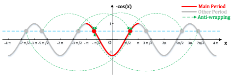
Figure 5: An interpretation diagram of the negative cosine function used as phase-related loss evaluation.

The total loss defined on phase spectra is

$$\mathcal{L}_{P}=\mathcal{L}_{IP}+\mathcal{L}_{GD}+\mathcal{L}_{PDT}.$$ (25)

The negative cosine function used in Equation 13, 19 and 24 is suitable for the definition of phase-related losses because of its three properties, including:

a) The parity. The negative cosine function is an even function that only cares about the absolute value of the phase difference and ignores its sign. This is reasonable since we expect the predicted phase to approximate the natural one regardless of the direction from which it is approached.

b) The periodicity. The negative cosine function has a period of $2\pi$, which can potentially avoid the issue caused by phase wrapping. As shown in Figure 4, the absolute values of the phase difference represented by the blue and red shaded areas are equal. However, in the actual calculation, the phase difference of the red shaded area (denoted by $P_{diff}^{wrapping}$) has a wrapping issue (i.e., $P_{diff}^{wrapping}\notin(-\pi,\pi]$) and its relationship with the phase difference of the blue shaded area (denoted by $P_{diff}^{no-wrapping}$) is

$$|P_{diff}^{no-wrapping}|=2\pi-|P_{diff}^{wrapping}|.$$ (26)

Then we can get

$$-\cos\left(P_{diff}^{no-wrapping}\right)=-\cos\left(P_{diff}^{wrapping}\right),$$ (27)

which indicates that the negative cosine function is an anti-wrapping function which can avoid the error caused by phase wrapping. Therefore, as shown in Figure 5, when calculating $\mathcal{L}_{IP}$, $\mathcal{L}_{GD}$ and $\mathcal{L}_{PTD}$, the negative cosine function potentially moves values outside $(-\pi,\pi]$ (i.e., gray dots) to the corresponding values within $(-\pi,\pi]$ (i.e., red dots), which performs anti-wrapping operation.

c) The monotonicity. The negative cosine function is monotonically increasing in interval $[0,\pi]$, ensuring that the smaller the absolute value of the phase difference, the smaller the loss.

III-C3 Losses defined on reconstructed STFT spectra

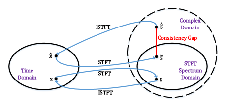
Figure 6: An interpretation diagram of the STFT spectrum consistency issue.

We first explain the short-time spectral inconsistency issue [44]. As shown in Figure 6, the STFT spectrum domain $\mathbb{S}^{F\times\left(\frac{N}{2}+1\right)}$ is a subset of the complex domain $\mathbb{C}^{F\times\left(\frac{N}{2}+1\right)}$, i.e., $\mathbb{S}^{F\times\left(\frac{N}{2}+1\right)}\subset\mathbb{C}^{F\times\left(\frac{N}{2}+1\right)}$. For a speech waveform $\bm{x}\in\mathbb{R}^{T}$, there must be

$$\bm{S}=STFT\left(\bm{x};L,\frac{T}{F},N\right)\in\mathbb{S}^{F\times\left(\frac{N}{2}+1\right)},$$ (28)

$$ISTFT\left(\bm{S};L,\frac{T}{F},N\right)=\bm{x}.$$ (29)

As shown in Figure 6, assume that the reconstructed STFT spectrum $\hat{\bm{S}}\in\mathbb{C}^{F\times\left(\frac{N}{2}+1\right)}-\mathbb{S}^{F\times\left(\frac{N}{2}+1\right)}$ (i.e., Equation 3), there must be

$$\hat{\bm{x}}=ISTFT\left(\hat{\bm{S}};L,\frac{T}{F},N\right),$$ (30)

$$STFT\left(\hat{\bm{x}};L,\frac{T}{F},N\right)=\tilde{\bm{S}}\in\mathbb{S}^{F\times\left(\frac{N}{2}+1\right)}\neq\hat{\bm{S}}.$$ (31)

At this point, an inconsistency problem occurs and the reconstructed $\hat{\bm{S}}$ is a “fake” STFT spectrum. The consistent spectrum corresponding to $\hat{\bm{S}}$ is $\tilde{\bm{S}}$. The difference between them is the consistency gap, which needs to be narrowed.

To alleviate short-time spectral inconsistency error, we define the following loss functions.

• STFT Consistency Loss: The STFT consistency loss aims to narrow the gap between $\hat{\bm{S}}$ and its consistent spectrum $\tilde{\bm{S}}$ and it is calculated as follows:

  $$\mathcal{L}_{C}=\mathbb{E}_{\left(\hat{\bm{S}},\tilde{\bm{S}}\right)}\overline{\left\{\left[Re(\hat{\bm{S}})-Re(\tilde{\bm{S}})\right]^{2}+\left[Im(\hat{\bm{S}})-Im(\tilde{\bm{S}})\right]^{2}\right\}}.$$ (32)

• Real and Imaginary Part Losses: The real and imaginary part losses are proposed to narrow the gap between $\hat{\bm{S}}$ and its natural spectrum $\bm{S}$, and they are defined as the mean L1 distance of the real parts and imaginary parts, respectively, i.e.,

  $$\mathcal{L}_{R}=\mathbb{E}_{\left(\hat{\bm{S}},\bm{S}\right)}\overline{|Re(\hat{\bm{S}})-Re(\bm{S})|},$$ (33)

  $$\mathcal{L}_{I}=\mathbb{E}_{\left(\hat{\bm{S}},\bm{S}\right)}\overline{|Im(\hat{\bm{S}})-Im(\bm{S})|}.$$ (34)

The total loss defined on reconstructed STFT spectra is

$$\mathcal{L}_{S}=\mathcal{L}_{C}+\lambda_{RI}\mathcal{L}_{R}+\lambda_{RI}\mathcal{L}_{I},$$ (35)

where $\lambda_{RI}$ is hyperparameter.

III-C4 Losses defined on final waveforms

The losses defined on final waveforms aim to narrow the gap between the final synthesized waveform $\hat{\bm{x}}$ through ISTFT (i.e., Equation 4) and the natural one $\bm{x}$. The losses are exactly the same as those used in HiFi-GAN [35], which adopts GAN-based training, including the GAN losses $\mathcal{L}_{GAN-G}$ and $\mathcal{L}_{GAN-D}$ for the generator and discriminator, respectively, feature matching loss $\mathcal{L}_{FM}$ and mel spectrogram loss $\mathcal{L}_{Mel}$. The total loss defined on final waveforms is

$$\mathcal{L}_{W}=L_{GAN-G}+\mathcal{L}_{FM}+\lambda_{Mel}\mathcal{L}_{Mel},$$ (36)

where $\lambda_{Mel}$ is hyperparameter.

III-C5 The final loss for model training

The training of the APNet vocoder follows the standard training process of GAN. The final generator loss is a linear combination of multilevel losses, i.e.,

$$\mathcal{L}_{G}=\lambda_{A}\mathcal{L}_{A}+\lambda_{P}\mathcal{L}_{P}+\lambda_{S}\mathcal{L}_{S}+\mathcal{L}_{W}.$$ (37)

where $\lambda_{A}$, $\lambda_{P}$ and $\lambda_{S}$ are hyperparameters. The discriminator loss is $\mathcal{L}_{D}=\mathcal{L}_{GAN-D}$.

III-C6 The inference process

The inference process strictly follows the all-frame-level calculation process from Equation 1 to Equation 4, as shown in the black part of Figure 2 (i.e., ignore the gray part).

IV Experiments

IV-A Experimental Setup

The LJSpeech dataset [45] was adopted in our experiments. We chose 10480 and 1310 utterances to construct the training set and the validation set, respectively, and the remaining 1310 utterances were used as the test set. The original waveforms in this dataset were downsampled to 16 kHz for our experiments. When extracting features (e.g., mel spectrograms, amplitude spectra, phase spectra and F0) from natural waveforms for vocoders, the window size was 20 ms (i.e., $L=320$), the window shift was 5 ms (i.e., $\frac{T}{F}=80$), and the FFT point number was 1024 (i.e., $N=1024$). For TTS experiments, we followed the open source implementation of a FastSpeech2-based acoustic model [46].

The subsequent experiments are organized as follows. We first compared our proposed APNet vocoder with other neural vocoders by analysis-synthesis (i.e., using natural acoustic features as input) and TTS (i.e., using acoustic features predicted by acoustic models as input) experiments. Then, we further conducted ablation experiments on the APNet vocoder to explore the role of the proposed parallel phase estimation architecture and loss functions.

IV-B Comparison among neural vocoders

TABLE I: Objective and subjective evaluation results of APNet, HiFi-GAN v1, HiFi-GAN v2, ISTFTNET, HiNet and MB-MelGAN on the test sets of the LJSpeech dataset. Here, “AS” and “TTS” represent analysis-synthesis and TTS tasks respectively. “$a\times$” represents $a\times$ real time. Objective results were calculated only on the analysis-synthesis task.

	SNR(dB)$\uparrow$	LAS-RMSE(dB)$\downarrow$	MCD(dB)$\downarrow$	F0-RMSE(cent)$\downarrow$	V/UV error(%)$\downarrow$	RTF (CPU)$\downarrow$	RTF (GPU)$\downarrow$	MOS(AS)$\uparrow$	MOS(TTS)$\uparrow$
Natural Speech	–	–	–	–	–	–	–	4.01$\pm$0.056	4.00$\pm$0.054
APNet	5.834	3.522	0.7729	19.83	3.142	0.068 (14.7$\times$)	0.0033 (303$\times$)	3.93$\pm$0.057	3.90$\pm$0.053
HiFi-GAN v1	7.528	3.207	0.5874	16.88	2.112	0.57 (1.76$\times$)	0.0034 (291$\times$)	3.99$\pm$0.056	3.90$\pm$0.060
HiFi-GAN v2	4.937	4.721	1.150	36.71	4.164	0.30 (3.28$\times$)	0.0027 (366$\times$)	3.86$\pm$0.057	3.87$\pm$0.059
ISTFTNET	4.824	4.905	1.252	38.04	4.490	0.077 (13.1$\times$)	0.0012 (817$\times$)	3.87$\pm$0.060	3.86$\pm$0.056
HiNet	3.429	5.394	1.515	38.78	5.301	5.6 (0.178$\times$)	0.22 (4.45$\times$)	3.82$\pm$0.062	–
MB-MelGAN	3.669	6.744	2.077	40.11	7.029	0.054 (18.4$\times$)	0.0015 (672$\times$)	3.82$\pm$0.062	3.80$\pm$0.061

We first conducted objective and subjective experiments to compare the performance of our proposed APNet vocoder and other neural vocoders. The descriptions of these vocoders are as follows.

• APNet: The proposed APNet vocoder. The input was 80-dimensional mel spectrograms. The residual convolution network in both ASP and PSP consisted of 3 parallel blocks (i.e., $P=3$), and each block was formed by concatenating 3 subblocks (i.e., $Q=3$). The kernel sizes of blocks were $k_{1}=3$, $k_{2}=7$ and $k_{3}=11$, and the dilation factors of subblocks within each block were $d_{*,1}=1$, $d_{*,2}=3$ and $d_{*,3}=5$. The channel size of the convolution operations in both ASP and PSP was 512, except for output layers. In particular, the channel size of the output layers was 513 (i.e., $\frac{N}{2}+1=513$). The hyperparameters for loss functions were set as $\lambda_{A}=\lambda_{Mel}=45$, $\lambda_{P}=100$, $\lambda_{S}=20$ and $\lambda_{RI}=2.25$. The model was trained using the AdamW optimizer [47] with $\beta_{1}=0.8$ and $\beta_{2}=0.99$ on a single Nvidia 3090Ti GPU. The learning rate decay was scheduled by a 0.999 factor in every epoch with an initial learning rate of 0.0002. The batch size was 16, and the truncated waveform length was 8000 samples (i.e., 0.5 s) for each training step. The model was trained until 3100 epochs.

• HiFi-GAN v1: The v1 version of the HiFi-GAN vocoder [35]. The input was 80-dimensional mel spectrograms. We reimplemented it using the open source implementation. We made small modifications to the open source code to fit our configurations. The upsampling ratios were set as $h_{1}=5$, $h_{2}=4$, $h_{3}=2$ and $h_{4}=2$. The training configuration is exactly the same as that of APNet.

• HiFi-GAN v2: The v2 version of the HiFi-GAN vocoder [35]. Compared with HiFi-GAN v1, it just reduced the channel size of the convolution operations from 512 to 128.

• ISTFTNET: The v2 version of the ISTFTNET vocoder [36]. The input was 80-dimensional mel spectrograms. We reimplemented it using the open source implementation. We made small modifications to the open source code to fit our configurations, and it was designed based on HiFi-GAN v2. The ISTFTNET passed 80-dimensional mel spectrograms through the first two residual networks incorporating upsampling layers of HiFi-GAN v2 (i.e., $h_{1}=5$ and $h_{2}=4$) and then outputted the amplitude and phase spectra at a 4 kHz sampling rate. The training configuration is exactly the same as that of APNet.

• HiNet: The HiNet vocoder [37] we previously proposed. The model configurations were the same as those used in the Baseline-HiNet model of our previous work [42]. The input included the 80-dimensional mel spectrograms, F0 extracted using YAPPT [48], and a voiced/unvoiced flag.

• MB-MelGAN: The multi-band MelGAN vocoder [38]. We reimplemented it using the open source implementation. We made small modifications to the open source code to fit our configurations. The model generated 4 subband waveforms with a 4 kHz sampling rate, and the upsampling ratios for each band were set as 5, 2 and 2. Finally, the full-band waveform was reconstructed by integrating these subband waveforms. This method significantly improved the inference efficiency compared with the original MelGAN [33].

We compared the performance of these vocoders using both objective and subjective evaluations. Five objective metrics used in our previous work [37] were adopted here, including the signal-to-noise ratio (SNR), which reflected the distortion of waveforms, root MSE (RMSE) of log amplitude spectra (denoted by LAS-RMSE), which reflected the distortion in the frequency domain, mel-cepstrum distortion (MCD), which described the distortion of mel-cepstra, RMSE of F0 (denoted by F0-RMSE), which reflected the distortion of F0, and V/UV error, which was the ratio between the number of frames with mismatched V/UV flags and the total number of frames. Among these metrics, SNR can be considered as an overall measurement of the distortions of both amplitude and phase spectra, while LAS-RMSE and MCD mainly present the distortion of amplitude spectra. To evaluate the inference efficiency, the real-time factor (RTF), which is defined as the ratio between the time consumed to generate speech waveforms and the duration of the generated speech, was also utilized as an objective metric. In our implementation, the RTF value was calculated as the ratio between the time consumed to generate all test sentences using a single Nvidia 3080Ti GPU or a single Intel Xeon E5-2680 CPU core and the total duration of the test set.

Regarding the subjective evaluation, mean opinion score (MOS) tests were conducted to compare the naturalness of these vocoders. In each MOS test, twenty test utterances synthesized by vocoders along with the natural utterances were evaluated by at least 30 native English listeners on the crowdsourcing platform of Amazon Mechanical Turk with anti-cheating considerations [49]. Listeners were asked to give a naturalness score between 1 and 5, and the score interval was 0.5. To compare the differences between the two vocoders individually, the ABX preference tests were also conducted on the Amazon Mechanical Turk platform and evaluated by at least 30 English native listeners. In each ABX test, twenty utterances were randomly selected from the test set synthesised by two comparative vocoders. The listeners were asked to judge which utterance in each pair had better speech quality or whether there was no preference. In addition to calculating the average preference scores, the $p$-value of a $t$-test was used to measure the significance of the difference between two vocoders.

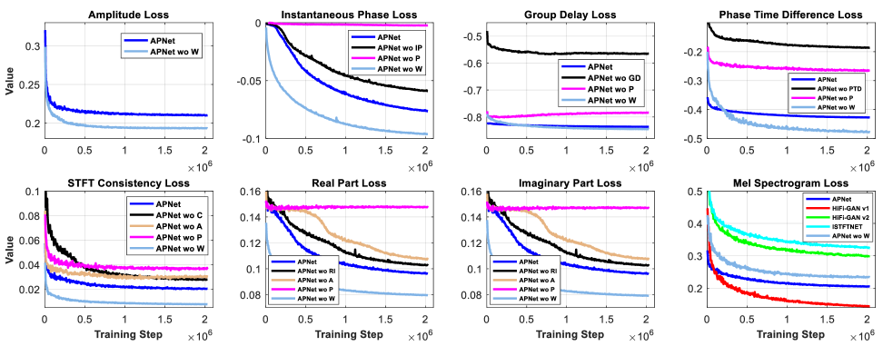
Figure 7: Loss curves for the validation set when training on the LJSpeech dataset.

The objective results on the test sets of the LJSpeech dataset for the analysis-synthesis task are listed in Table I. It is obvious that HiFi-GAN v1 achieved the highest scores for all objective metrics. Our proposed APNet outperformed HiFi-GAN v2, ISTFTNET, HiNet and MB-MelGAN on all objective metrics, which demonstrates the strong performance on synthesized speech quality of the proposed methods. For more evidence, Figure 7 draws the curves of the losses on the validation set as a function of training steps on the LJSpeech dataset. The APNet, HiFi-GAN v1, HiFi-GAN v2 and ISTFTNET are comparable because they all employ similar training modes and the common losses (e.g., the mel spectrogram loss) defined on the waveform. Consistent with the previous observations, the mel spectrogram loss convergence value of APNet was higher than that of HiFi-GAN v1 but significantly lower than that of HiFi-GAN v2 and ISTFTNET. Besides, we can see that all losses in APNet converged normally.

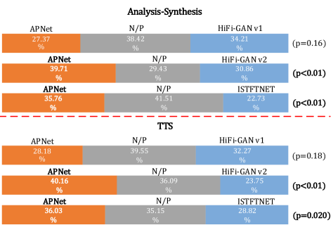
Figure 8: Average preference scores (%) of ABX tests on speech quality between APNet and three other vocoders (i.e., HiFi-GAN v1, HiFi-GAN v2 and ISTFTNET), where N/P stands for “no preference” and $p$ denotes the $p$-value of a $t$-test between two vocoders.

The subjective MOS test results and RTFs on the test set of the LJSpeech dataset are also listed in Table I. Interestingly, the gap between our proposed APNet and the state-of-the-art HiFi-GAN v1 was only 0.06 MOS scores for the analysis-synthesis task. The MOS scores of APNet and HiFi-GAN v1 were very close to those of ground truth. For the TTS task, the APNet and HiFi-GAN v1 had similar MOS scores, which indicated that the proposed APNet vocoder was robust to the acoustic features predicted by acoustic models. Our proposed APNet also had better synthesized speech quality than HiFi-GAN v2, ISTFTNET, HiNet and MB-MelGAN regarding the MOS scores for both analysis-synthesis and TTS tasks. The HiNet was discarded in the TTS task because it still required additional F0 input. To further investigate the quality differences among APNet, HiFi-GAN v1, HiFi-GAN v2 and ISTFTNET, we additionally performed several groups of ABX tests to compare the APNet with HiFi-GAN v1, HiFi-GAN v2 and ISTFTNET, separately. The results of the ABX tests are shown in Figure 8. The performance of APNet was not significantly different from that of HiFi-GAN v1 ($p>0.05$) but significantly better than that of HiFi-GAN v2 and ISTFTNET ($p<0.05$), both for analysis-synthesis and TTS tasks. According to the listener’s feedback, a few sentences of HiFi-GAN v2 and ISTFTNET were slightly jittery or blurred. Regarding the RTF, the ISTFTNET showed the fastest inference speed on GPU. The inference speed of our proposed APNet on GPU was similar to the two versions of HiFi-GAN, and it achieved approximately 14x real-time inference on CPU, significantly faster than the two versions of HiFi-GAN. The possible reason is that the CPU does not support parallel acceleration generation, resulting in slower direct waveform inference. Although the ISTFTNET and MB-MelGAN had similar inference speeds on the CPU as APNet, their synthesized speech quality was noticeably worse. The inference speed of HiNet was the slowest, either on GPU or CPU. By comparing HiNet and APNet, we can see that the APNet vocoder has completely surpassed the HiNet vocoder in terms of both synthesized speech quality and inference efficiency, thanks to the introduction of the new frame-level PSP, as well as the joint training mode of ASP and PSP. In conclusion, these experimental results confirm that our proposed APNet vocoder achieved synthesized speech quality comparable to HiFi-GAN but significantly improves the inference efficiency on CPU, benefiting from avoiding direct prediction of waveforms in our methods.

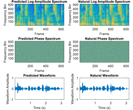
Figure 9: Visualized comparison of log amplitude spectrum, phase spectrum and waveform predicted by APNet with the natural ones for a test utterance.

Figure 9 draws the color maps of the log amplitude spectrum and wrapped phase spectrum predicted by the ASP and PSP in APNet and the reconstructed waveform for a test utterance. The corresponding natural ones are also drawn in Figure 9 for comparison. Obviously, the predicted amplitude spectrum successfully recovered spectral information such as F0 and harmonics, but it was slightly over smooth compared to the natural amplitude spectrum. Although it was difficult to see specific information from the color map of the phase spectrum, the overall distribution of the predicted phase spectrum was generally similar to the natural one by observing Figure 9. In addition, the APNet vocoder also restored the overall waveform contour precisely compared with the natural one.

IV-C Ablation studies

TABLE II: Objective evaluation results of APNet and its ablated variants on the test set of the LJSpeech dataset for the analysis-synthesis task.

Descriptions	Vocoders	SNR(dB)$\uparrow$	LAS-RMSE(dB)$\downarrow$	MCD(dB)$\downarrow$	F0-RMSE(cent)$\downarrow$	V/UV error(%)$\downarrow$
Original	APNet	5.834	3.522	0.7729	19.83	3.142
Ablate Parallel Phase Estimation Architecture	APNet wo PPEA	3.811	3.199	0.9967	38.35	5.842
Ablate Amplitude-related Loss	APNet wo A	5.289	3.708	0.9382	25.41	3.696
Ablate Phase-related Losses	APNet wo IP	5.605	3.699	0.8188	20.83	3.587
	APNet wo GD	6.323	4.091	0.9630	18.93	3.127
	APNet wo PTD	5.295	3.434	0.8843	26.71	4.606
	APNet wo P	4.163	3.683	0.9920	40.51	5.821
Ablate STFT Spectrum-related Losses	APNet wo C	6.077	3.712	0.7884	19.09	2.916
	APNet wo RI	5.849	3.681	0.7668	20.58	3.366
Ablate Waveform-related Losses	APNet wo W	6.447	5.421	1.269	14.81	2.390

We then conducted several ablation experiments to explore the roles of the proposed parallel phase estimation architecture and loss functions in the APNet vocoder. We utilized some of the objective metrics used in the previous section and the subjective ABX preference test to compare APNet with its ablated variants. The objective and subjective results are shown in Table II and Figure 10, respectively. Ablation experiments were performed only on the analysis-synthesis task.

IV-C1 Ablate the parallel phase estimation architecture

Here is one ablated vocoder for comparison with APNet, i.e.,

• APNet wo PPEA: Removing the parallel phase estimation architecture (i.e., two parallel output layers and phase calculation formula $\bm{\Phi}$) from APNet. The output of the residual convolution network in the PSP passes through a linear layer without activation to predict the phase spectra.

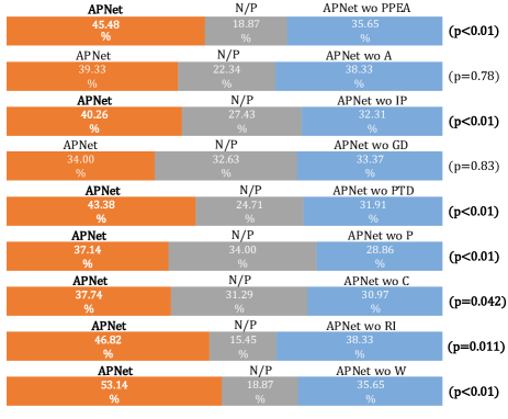
Figure 10: Average preference scores (%) of ABX tests on speech quality between APNet and its ablated variants, where N/P stands for “no preference” and $p$ denotes the $p$-value of a $t$-test between two vocoders.

Unsurprisingly, the APNet outperformed APNet wo PPEA very significantly according to both objective and subjective results ($p<0.01$) in Table II and Figure 10. In Figure 11, we drew the color maps of the phase spectra predicted by the PSP in APNet and APNet wo PPEA. Obviously, the APNet wo PPEA failed to control the range of the predicted phase which overflowed the principal value interval $(-\pi,\pi]$. This led to a loss of phase prediction accuracy and degradation of synthesized speech quality, thus confirming the effectiveness of our proposed parallel phase estimation architecture.

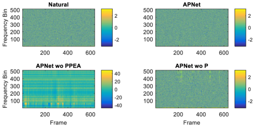
Figure 11: A comparison among the natural phase spectrum and phase spectra predicted by the PSP in APNet, APNet wo PPEA and APNet wo P for a test utterance.

IV-C2 Ablate the amplitude-related loss

Here is one ablated vocoder for comparison with APNet, i.e.,

• APNet wo A: Removing the amplitude loss $\mathcal{L}_{A}$ from APNet at the training stage.

Table II shows that the APNet wo A attenuated all objective metrics compared with APNet. In addition, the amplitude loss $\mathcal{L}_{A}$ of APNet wo A on the validation set did not converge and stabilized at approximately 8.5, while that of APNet converged to approximately 0.2, as shown in Figure 7. From Figure 7, we can also see that removing $\mathcal{L}_{A}$ also negatively affected the convergence of the STFT spectrum-related losses (i.e., $\mathcal{L}_{C}$, $\mathcal{L}_{R}$ and $\mathcal{L}_{I}$). However, there was no significant subjective difference ($p>0.05$) between APNet and APNet wo A considering the sense of hearing, as shown in Figure 10. For more evidence, Figure 12 draws the spectrograms of the speech generated by APNet and APNet wo A. Obviously, the spectrogram of APNet wo A exhibited high-frequency horizontal streaks (see the blue boxes in Figure 12), which may degrade the objective results. However, this issue was not sensitive to hearing according to the subjective results.

IV-C3 Ablate the phase-related losses

Here are four ablated vocoders for comparison with APNet, i.e.,

• APNet wo IP: Removing the instantaneous phase loss $\mathcal{L}_{IP}$ from APNet at the training stage.

• APNet wo GD: Removing the group delay loss $\mathcal{L}_{GD}$ from APNet at the training stage.

• APNet wo PTD: Removing the phase time difference loss $\mathcal{L}_{PTD}$ from APNet at the training stage.

• APNet wo P: Removing $\mathcal{L}_{IP}$, $\mathcal{L}_{GD}$ and $\mathcal{L}_{PTD}$ from APNet at the training stage (i.e., no losses directly defined on phase spectra).

From Table II, we can see that the APNet wo IP and APNet wo PTD degraded most objective metrics. However, the APNet wo GD even improved the SNR and F0-related metrics, which requires further investigation. Removing all the phase-related losses (i.e., APNet wo P) caused a sharp degradation in all objective metrics. Considering the convergence curves shown in Figure 7, we can see that removing a loss function at the training stage was bound to negatively affect the convergence of this loss value on the validation set. The instantaneous phase loss curves of the APNet wo IP and APNet wo P also suggested that the phase difference losses (i.e., $\mathcal{L}_{GD}$ and $\mathcal{L}_{PTD}$) had a positive effect on the instantaneous phase loss (i.e., $\mathcal{L}_{IP}$). Interestingly, the two phase difference losses were mutually exclusive by comparing the APNet wo P with APNet wo GD and APNet wo PTD using the group delay loss curve and phase time difference loss curve, respectively in Figure 7. In addition, removing phase-related losses also significantly affected the convergence of the STFT spectrum-related losses (i.e., $\mathcal{L}_{C}$, $\mathcal{L}_{R}$ and $\mathcal{L}_{I}$). It is reasonable that the amplitude- and phase-related losses facilitated the convergence of the STFT spectrum-related losses. By comparing the APNet wo A and APNet wo P, we can also confirm that the phase-related losses contributed more to improving STFT spectrum consistency than the amplitude-related loss.

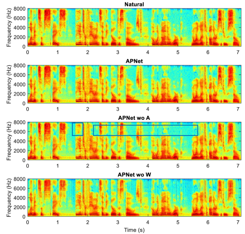
Figure 12: A comparison among the spectrograms of the natural speech and speeches generated by APNet, APNet wo A and APNet wo W.

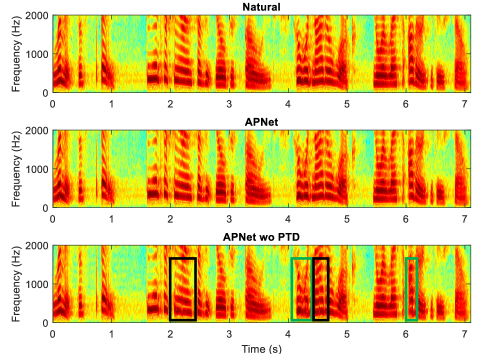
Figure 13: A comparison between the spectrograms of the natural speech and speeches generated by APNet and APNet wo PTD for the interpretation of the spectral discontinuity.

Regarding the subjective results in Figure 10, the APNet wo IP, APNet wo PTD and APNet wo P outperformed the APNet very significantly ($p<0.01$). However, there was no significant difference ($p>0.05$) between the APNet and APNet wo GD. Although the APNet wo GD significantly degraded the amplitude spectra according to the LAS-RMSE and MCD values in Table II, the amplitude distortion might not cause a significant decrease in the sense of hearing. This finding was similar to the conclusion in subsection IV-C2. These results suggested that the degree of importance of the three losses was $\mathcal{L}_{PTD}>\mathcal{L}_{IP}>\mathcal{L}_{GD}$. We can also draw the conclusion that these three losses should be combined and balanced during training, which was more helpful to improve the phase prediction ability of PSP, rather than using any of these losses alone. In addition, we found that a common issue existing in these four ablated vocoders was spectral discontinuity. We took the APNet wo PTD as an example and drew the spectrograms in Figure 13. Discontinuity issues usually occurred at low frequencies, mainly including spectral blurring (green boxes in Figure 13) and spectral splitting (black boxes in Figure 13), resulting in slurred and clicky pronunciation. This was due to the inconsistency of the STFT spectrum reconstructed by the predicted amplitude and phase spectra. Therefore, phase-related losses facilitated the alleviation of STFT spectral inconsistency. Finally, we also compared the phase spectra predicted by the PSP in APNet and APNet wo P in Figure 11. Obviously, there existed horizontal stripes in the phase spectra of APNet wo P at the high frequency band, resulting in the degradation of phase prediction accuracy, which further demonstrated the effectiveness of our proposed phase-related losses.

IV-C4 Ablate the STFT spectrum-related losses

Here are two ablated vocoders for comparison with APNet, i.e.,

• APNet wo C: Removing the STFT consistency loss $\mathcal{L}_{C}$ from APNet at the training stage.

• APNet wo RI: Removing the real part loss $\mathcal{L}_{R}$ and imaginary part loss $\mathcal{L}_{I}$ from APNet at the training stage.

From Table II, we can see that the objective results of the APNet wo C and APNet wo RI are similar to those of the APNet, which requires further investigation. By observing Figure 7, although removing losses $\mathcal{L}_{C}$, $\mathcal{L}_{R}$ and $\mathcal{L}_{I}$ during the training stage caused an increase in the corresponding losses on the validation set, their increase degrees were smaller than that of the phase-related losses (i.e., $\mathcal{L}_{IP}$, $\mathcal{L}_{GD}$ and $\mathcal{L}_{GDT}$). This suggested that the STFT spectrum-related losses played an auxiliary role in improving the consistency of the STFT spectra. Regarding the subjective results shown in Figure 10, the APNet outperformed both the APNet wo C and APNet wo RI significantly ($p<0.05$). Other findings were that the APNet wo C and APNet wo RI also exhibited spectral discontinuity issues, as shown in Figure 13, which may be the reason for the decreased sense of hearing. Therefore, the STFT spectrum-related losses were effective for improving the synthesized speech quality and alleviating the STFT spectral inconsistency issues.

IV-C5 Ablate the waveform-related losses

Here is one ablated vocoder for comparison with APNet, i.e.,

• APNet wo W: Removing all losses defined on the final waveform (i.e., $L_{GAN-G}$, $L_{GAN-D}$, $L_{FM}$ and $L_{Mel}$) from APNet at the training stage.

Interestingly, the APNet wo W degraded the LAS-RMSE and MCD very significantly, but it improved the other three objective metrics, which requires further investigation. By observing Figure 7, we found that the APNet wo W facilitated the convergence of all losses except the mel spectrogram loss. This finding means that waveform-related losses restricted the independent learning of the ASP and PSP in APNet. Removing waveform-related losses pushed the ASP and PSP to local optima but ignored the global optima of the final reconstructed waveforms. As expected, the APNet outperformed APNet wo W very significantly ($p<0.01$) according to the subjective results in Figure 10. Figure 12 also draws the spectrograms of the speech generated by APNet wo W. There were obvious vertical lines existing in the spectrogram of APNet wo W, which caused annoying clicking noises and degraded the amplitude-related objective results (i.e., the LAS-RMSE and MCD) and subjective results. However, the vertical line issue did not destroy F0, as shown in Figure 12, which may be the reason why the objective metrics related to F0 have not deteriorated. However, after removing waveform-related losses, the model training efficiency was improved by approximately 8 times. This finding is encouraging and points the way for our future work to improve the training efficiency of the APNet vocoder.

V Conclusion

In this paper, we proposed a novel neural vocoder called APNet, which incorporates the direct prediction of speech amplitude and phase spectra. The APNet vocoder consists of an ASP and a PSP, which both perform at the frame level. The ASP employs a residual convolution network to predict the log amplitude spectra from input acoustic features. The PSP introduces a parallel phase estimation architecture on the basis of ASP and successfully realizes direct phase spectrum prediction from acoustic features. Some well-designed loss functions are defined on the predicted log amplitude spectra, phase spectra, reconstructed STFT spectra and final waveforms, and jointly train the ASP and PSP. Experimental results show that our proposed APNet vocoder achieved approximately 14x real-time inference efficiency on a CPU, which was 8x faster than HiFi-GAN v1 when its synthesized speech quality was comparable to HiFi-GAN v1. Ablation studies also demonstrated the effectiveness of the proposed parallel phase estimation architecture and loss functions.

In future work, we will 1) adapt the APNet vocoder to other configurations (e.g., increase the frame shift, increase the waveform sampling rate, etc.); 2) improve the training efficiency of the APNet vocoder; and 3) apply the proposed phase prediction method to other speech generation tasks, such as speech enhancement (SE), speech bandwidth extension (BWE), etc.

References

- [1] H. Zen, K. Tokuda, and A. W. Black, “Statistical parametric speech synthesis,” Speech Communication, vol. 51, no. 11, pp. 1039–1064, 2009.
- [2] Y. Wang, R. Skerry-Ryan, D. Stanton, Y. Wu, R. J. Weiss, N. Jaitly, Z. Yang, Y. Xiao, Z. Chen, S. Bengio et al., “Tacotron: Towards end-to-end speech synthesis,” in Proc. Interspeech, 2017, pp. 4006–4010.
- [3] J. Shen, R. Pang, R. J. Weiss, M. Schuster, N. Jaitly, Z. Yang, Z. Chen, Y. Zhang, Y. Wang, R. Skerrv-Ryan et al., “Natural TTS synthesis by conditioning wavenet on mel spectrogram predictions,” in Proc. ICASSP, 2018, pp. 4779–4783.
- [4] N. Li, S. Liu, Y. Liu, S. Zhao, and M. Liu, “Neural speech synthesis with transformer network,” in Proc. AAAI, vol. 33, no. 01, 2019, pp. 6706–6713.
- [5] K. Tokuda, Y. Nankaku, T. Toda, H. Zen, J. Yamagishi, and K. Oura, “Speech synthesis based on hidden Markov models,” Proceedings of the IEEE, vol. 101, no. 5, pp. 1234–1252, 2013.
- [6] H. Zen, A. Senior, and M. Schuster, “Statistical parametric speech synthesis using deep neural networks,” in Proc. ICASSP, 2013, pp. 7962–7966.
- [7] Y. Fan, Y. Qian, F.-L. Xie, and F. K. Soong, “TTS synthesis with bidirectional LSTM based recurrent neural networks,” in Proc. Interspeech, 2014, pp. 1964–1968.
- [8] H. Dudley, “The vocoder,” Bell Labs Record, vol. 18, no. 4, pp. 122–126, 1939.
- [9] H. Kawahara, I. Masuda-Katsuse, and A. De Cheveigne, “Restructuring speech representations using a pitch-adaptive time–frequency smoothing and an instantaneous-frequency-based f0 extraction: Possible role of a repetitive structure in sounds,” Speech communication, vol. 27, no. 3, pp. 187–207, 1999.
- [10] M. Morise, F. Yokomori, and K. Ozawa, “WORLD: A vocoder-based high-quality speech synthesis system for real-time applications,” IEICE Transactions on Information and Systems, vol. 99, no. 7, pp. 1877–1884, 2016.
- [11] L.-J. Liu, Z.-H. Ling, Y. Jiang, M. Zhou, and L.-R. Dai, “WaveNet vocoder with limited training data for voice conversion,” in Proc. Interspeech, 2018, pp. 1983–1987.
- [12] H. Liu, W. Choi, X. Liu, Q. Kong, Q. Tian, and D. Wang, “Neural vocoder is all you need for speech super-resolution,” arXiv preprint arXiv:2203.14941, 2022.
- [13] P. Andreev, A. Alanov, O. Ivanov, and D. Vetrov, “HiFi++: a unified framework for neural vocoding, bandwidth extension and speech enhancement,” arXiv preprint arXiv:2203.13086, 2022.
- [14] A. v. d. Oord, S. Dieleman, H. Zen, K. Simonyan, O. Vinyals, A. Graves, N. Kalchbrenner, A. Senior, and K. Kavukcuoglu, “WaveNet: A generative model for raw audio,” in 9th ISCA Speech Synthesis Workshop, 2016, pp. 125–125.
- [15] S. Mehri, K. Kumar, I. Gulrajani, R. Kumar, S. Jain, J. Sotelo, A. Courville, and Y. Bengio, “SampleRNN: An unconditional end-to-end neural audio generation model,” in Proc. ICLR, 2017.
- [16] N. Kalchbrenner, E. Elsen, K. Simonyan, S. Noury, N. Casagrande, E. Lockhart, F. Stimberg, A. Oord, S. Dieleman, and K. Kavukcuoglu, “Efficient neural audio synthesis,” in Proc. ICML, 2018, pp. 2410–2419.
- [17] A. Tamamori, T. Hayashi, K. Kobayashi, K. Takeda, and T. Toda, “Speaker-dependent WaveNet vocoder,” in Proc. Interspeech, 2017, pp. 1118–1122.
- [18] T. Hayashi, A. Tamamori, K. Kobayashi, K. Takeda, and T. Toda, “An investigation of multi-speaker training for WaveNet vocoder,” in Proc. ASRU, 2017, pp. 712–718.
- [19] N. Adiga, V. Tsiaras, and Y. Stylianou, “On the use of WaveNet as a statistical vocoder,” in Proc. ICASSP, 2018, pp. 5674–5678.
- [20] Y. Ai, H.-C. Wu, and Z.-H. Ling, “SampleRNN-based neural vocoder for statistical parametric speech synthesis,” in Proc. ICASSP, 2018, pp. 5659–5663.
- [21] Y. Ai, J.-X. Zhang, L. Chen, and Z.-H. Ling, “DNN-based spectral enhancement for neural waveform generators with low-bit quantization,” in Proc. ICASSP, 2019, pp. 7025–7029.
- [22] J. Lorenzo-Trueba, T. Drugman, J. Latorre, T. Merritt, B. Putrycz, R. Barra-Chicote, A. Moinet, and V. Aggarwal, “Towards achieving robust universal neural vocoding,” Proc. Interspeech, pp. 181–185, 2019.
- [23] A. v. d. Oord, Y. Li, I. Babuschkin, K. Simonyan, O. Vinyals, K. Kavukcuoglu, G. v. d. Driessche, E. Lockhart, L. C. Cobo, F. Stimberg et al., “Parallel WaveNet: Fast high-fidelity speech synthesis,” in Proc. ICML, 2018, pp. 3918–3926.
- [24] W. Ping, K. Peng, and J. Chen, “ClariNet: Parallel wave generation in end-to-end text-to-speech,” in Proc. ICLR, 2019.
- [25] R. Prenger, R. Valle, and B. Catanzaro, “WaveGlow: A flow-based generative network for speech synthesis,” in Proc. ICASSP, 2019, pp. 3617–3621.
- [26] W. Ping, K. Peng, K. Zhao, and Z. Song, “WaveFlow: A compact flow-based model for raw audio,” in Proc. ICML, 2020, pp. 7706–7716.
- [27] L. Juvela, B. Bollepalli, V. Tsiaras, and P. Alku, “GlotNet-A raw waveform model for the glottal excitation in statistical parametric speech synthesis,” IEEE/ACM Transactions on Audio, Speech, and Language Processing, vol. 27, no. 6, pp. 1019–1030, 2019.
- [28] J.-M. Valin and J. Skoglund, “LPCNet: Improving neural speech synthesis through linear prediction,” in Proc. ICASSP, 2019, pp. 5891–5895.
- [29] X. Wang, S. Takaki, and J. Yamagishi, “Neural source-filter-based waveform model for statistical parametric speech synthesis,” in Proc. ICASSP, 2019, pp. 5916–5920.
- [30] I. Goodfellow, J. Pouget-Abadie, M. Mirza, B. Xu, D. Warde-Farley, S. Ozair, A. Courville, and Y. Bengio, “Generative adversarial nets,” in Proc. NeurIPS, 2014, pp. 2672–2680.
- [31] C. Donahue, J. McAuley, and M. Puckette, “Adversarial audio synthesis,” in Proc. ICLR, 2018.
- [32] M. Bińkowski, J. Donahue, S. Dieleman, A. Clark, E. Elsen, N. Casagrande, L. C. Cobo, and K. Simonyan, “High fidelity speech synthesis with adversarial networks,” in Proc. ICLR, 2019.
- [33] K. Kumar, R. Kumar, T. de Boissiere, L. Gestin, W. Z. Teoh, J. Sotelo, A. de Brébisson, Y. Bengio, and A. C. Courville, “MelGAN: Generative adversarial networks for conditional waveform synthesis,” Advances in neural information processing systems, vol. 32, 2019.
- [34] R. Yamamoto, E. Song, and J.-M. Kim, “Parallel WaveGan: A fast waveform generation model based on generative adversarial networks with multi-resolution spectrogram,” in Proc. ICASSP, 2020, pp. 6199–6203.
- [35] J. Kong, J. Kim, and J. Bae, “HiFi-GAN: Generative adversarial networks for efficient and high fidelity speech synthesis,” Advances in Neural Information Processing Systems, vol. 33, pp. 17 022–17 033, 2020.
- [36] T. Kaneko, K. Tanaka, H. Kameoka, and S. Seki, “ISTFTNET: Fast and lightweight mel-spectrogram vocoder incorporating inverse short-time fourier transform,” in Proc. ICASSP, 2022, pp. 6207–6211.
- [37] Y. Ai and Z.-H. Ling, “A neural vocoder with hierarchical generation of amplitude and phase spectra for statistical parametric speech synthesis,” IEEE/ACM Transactions on Audio, Speech, and Language Processing, vol. 28, pp. 839–851, 2020.
- [38] G. Yang, S. Yang, K. Liu, P. Fang, W. Chen, and L. Xie, “Multi-band MelGAN: Faster waveform generation for high-quality text-to-speech,” in Proc. SLT, 2021, pp. 492–498.
- [39] Y. Ai and Z.-H. Ling, “Knowledge-and-data-driven amplitude spectrum prediction for hierarchical neural vocoders,” in Proc. Interspeech, 2020, pp. 190–194.
- [40] Y. Ai, X. Wang, J. Yamagishi, and Z.-H. Ling, “Reverberation modeling for source-filter-based neural vocoder,” in Proc. Interspeech, 2020, pp. 3560–3564.
- [41] Y. Ai, H. Li, X. Wang, J. Yamagishi, and Z. Ling, “Denoising-and-dereverberation hierarchical neural vocoder for robust waveform generation,” in Proc. SLT, 2021, pp. 477–484.
- [42] Y. Ai, Z.-H. Ling, W.-L. Wu, and A. Li, “Denoising-and-dereverberation hierarchical neural vocoder for statistical parametric speech synthesis,” IEEE/ACM Transactions on Audio, Speech, and Language Processing, vol. 30, pp. 2036–2048, 2022.
- [43] A. L. Maas, A. Y. Hannun, and A. Y. Ng, “Rectifier nonlinearities improve neural network acoustic models,” in Proc. ICML, vol. 30, no. 1, 2013, p. 3.
- [44] J. Le Roux, H. Kameoka, N. Ono, and S. Sagayama, “Fast signal reconstruction from magnitude STFT spectrogram based on spectrogram consistency,” in Proc. DAFx, vol. 10, 2010, pp. 397–403.
- [45] K. Ito and L. Johnson, “The LJ speech dataset,” 2017. [Online]. Available: https://keithito.com/LJ-Speech-Dataset/
- [46] Y. Yasuda, X. Wang, S. Takaki, and J. Yamagishi, “Investigation of enhanced tacotron text-to-speech synthesis systems with self-attention for pitch accent language,” in Proc. ICASSP, 2019, pp. 6905–6909.
- [47] I. Loshchilov and F. Hutter, “Decoupled weight decay regularization,” in Proc. ICLR, 2018.
- [48] K. Kasi and S. A. Zahorian, “Yet another algorithm for pitch tracking,” in Proc. ICASSP, vol. 1, 2002, pp. 361–364.
- [49] S. Buchholz and J. Latorre, “Crowdsourcing preference tests, and how to detect cheating,” in Proc. Interspeech, 2011, pp. 3053–3056.