Sustaining quasi de-Sitter inflation with bulk viscosity

Abstract

We here investigate bulk-viscosity driven quasi de-Sitter inflation, that is, the period of accelerated expansion in the early universe during which $-\dot{H}\ll H^{2}$, with $H(t)$ being the Hubble expansion rate. We do so in the framework of a causal theory of relativistic hydrodynamics that takes into account non-equilibrium effects associated to bulk viscosity that may be present as the early universe undergoes an accelerated expansion. In this framework, the existence of a quasi de-Sitter universe emerges as a natural consequence of the presence of bulk viscosity, without requiring to introduce additional scalar fields. As a result, the equation of state, determined by numerically solving the generalized momentum-conservation equation involving bulk-viscosity pressure turns out to be time-dependent. The transition timescale characterising its departure from an exact de-Sitter phase is intricately related to the magnitude of the bulk viscosity. We examine the properties of the new equation of state, as well as the transition timescale in presence of bulk-viscosity pressure. In addition, we construct a fluid description of inflation and demonstrated that, in the context of the causal formalism, it is equivalent to the scalar field theory of inflation. Our analysis also shows that the slow-roll conditions are realised in the bulk-viscosity supported model of inflation. Finally, we examine the viability of our model by computing the inflationary observables, namely, the spectral index and the tensor-to-scalar ratio of the curvature perturbations, and compare them with a number of different observations finding good agreement in most cases.

1 Introduction

The inflationary paradigm plays a pivotal role in modern cosmology which relies on the idea that the early universe after Big-Bang underwent nearly exponential expansion within a very short interval of time [1, 2, 3]. While successfully providing explanations to all the drawbacks of the Big-Bang cosmology, inflation also presents natural explanations concerning large-scale structure formation of the observable universe and the distribution of the galaxies [4, 5, 6]. The predictions of inflation associated to the temperature anisotropies measured in the cosmic microwave background radiation are well-supported by data sources, e.g., , from the BICEP2 experiments [7], Wilkinson Microwave Anisotropy Probe (WMAP) [8, 9, 10, 11] and Planck results [12, 13].

The scalar field description is a most commonly adopted approach for addressing inflation, where a scalar field, known as the “inflaton” field and a specific a potential is responsible for driving the accelerated expansion of the early universe [14]. In the last few decades, extensive studies have been carried out for addressing different facets of inflation using single scalar fields models [15, 16, 17], multi-scalar field models [18, 19], braneworld and string-theory scenarios [20, 21] in the framework of both Einstein’s theory and alternative theories of gravity [22, 23, 24].

An alternative approach to the scalar-field description is one in which inflation is governed by bulk-viscosity pressure providing sufficient amount of negative pressure that is essential for the accelerated expansion. In this approach, the dynamical equations are described by a relativistic theory of non-perfect cosmological fluids [25, 26, 27] (for recent works we refer [28, 29, 30, 31, 32, 33, 34, 35] and references therein). A well-developed and commonly employed relativistic theory of non-perfect fluids is due to Müller [36], Israel and Stewart [37, 38] and is normally referred to as the MIS theory. In this phenomenological formulation, which is hyperbolic and stable, relies on the assumption that dissipative fluxes (in the form of bulk viscosity, shear viscosity, heat flux and charge flow) in the system amounts to small departures from equilibrium [39, 40] (see also [41] for an introduction). Consequently, the effects of these fluxes may be treated as perturbations to the equilibrium quantities.

Although the MIS theory is a valid relativistic hydrodynamical description of non-perfect fluids, it does not provide a reasonable description when applied to the epoch of accelerated expansion of the early universe. This is because the basic assumptions behind the MIS theory (small departures away from equilibrium) are no longer respected in this epoch. More specifically, during inflation the Strong Energy Condition (SEC) is violated, thus allowing bulk-viscosity pressure to be comparable with the equilibrium pressure and energy density of the cosmological fluid. As a result, the departures from the equilibrium are large to instil sufficiently large non-equilibrium effects and the universe does not remain close to equilibrium during the inflationary period. Thus, the MIS formalism may fail to provide an accurate description of the cosmological evolution during inflation.

Due to lack of a well-understood theory of non-equilibrium relativistic hydrodynamics valid during inflation, the out-of-equilibrium effects are accommodated in a phenomenological model first put forward by Maartens and Mendez [42], who proposed a generalisation of the MIS theory by taking into considerations of SEC. While preserving causality, the approach proposed in [42] introduces a new characteristic timescale that is non-vanishing when non-equilibrium effects are present. As a result, the modified evolution equation of the bulk-viscosity pressure contain an additional coefficient responsible for far-from-equilibrium effects. There are several important advantages of the formalism presented by Maartens and Mendez [42]. First, the MIS theory is correctly retrieved in the regime when the departures from the equilibrium are small. Second, the theory ensures the validity of the second law of thermodynamics hence the entropy production rate remains positive. Third, an upper bound on maximum value of the bulk-viscosity pressure exists and is compatible with the second law of thermodynamics.

We have here extended the work of Maartens and Mendez [42] by relaxing the exact de-Sitter condition so as to assess whether a quasi de-Sitter expansion of the early universe, i.e., an inflationary scenario characterised by $-\dot{H}\ll H^{2}$, can be actually sustained by bulk viscosity. To this scope, we introduce an effective equation of state (EOS), where the relation between the pressure and the energy density is no longer constant at all times but becomes time-dependent as a result of non-equilibrium effects and a time-dependent bulk viscous stress. However, as a new equilibrium is reached, the EOS stops evolving and a new constant relation emerges between the pressure and the energy density. To quantify this behaviour, our model is described in terms of three parameters: the coefficient of bulk viscosity, the characteristic timescale of non-equilibrium effects, and the timescale relating between equilibrium pressure and energy density of the cosmological fluid.

In this way, we find that the quasi de-Sitter inflation is a natural outcome of the presence of a nonzero bulk viscosity and hence does not require the need for an inflaton field. In particular, the universe always exhibits departure from the exact de-Sitter universe, so that, as long as the EOS is time-dependent, an exact de-Sitter universe cannot exist. The evolution of the transition timescale of the modified EOS from the exact de-Sitter solution is found to depend on the variation of each of the three aforementioned parameters of the model. As an example, we find that this transition timescale during the quasi de-Sitter expansion is inversely proportional to the magnitude of the bulk viscosity. On the other hand, the timescale over which non-equilibrium effects are present, is larger than previously found, even though they do not have a significant impact in altering the qualitative behaviour of equation of the state.

Furthermore, our analysis reveals as the universe evolves during inflation, the absolute magnitude of the bulk-viscosity pressure diminishes before settling to a small and nearly constant value. We have determined admissible regions of the parameters of the model under the quasi de Sitter conditions and on comparing with the exact de-Sitter case, we find that the admissible parameter region of one of the parameters ($w_{0}$, see below) is found to be considerably larger than what computed so far. Finally, as a test of our model, we compute the inflationary observables, i.e., the spectral index and the tensor-to-scalar ratio of the curvature perturbations, and compare them with the observations. In this way, we find that while our predictions are compatible with non-Planck based observations, they are in tension based on the Planck data.

The paper is organised as follows. Section 2 provides an overview on the bulk-viscosity driven inflation and is devoted to developing the mathematical background for the paper. In Sec. 3 the numerical results are presented which are obtained by solving the generalized momentum-conservation equation in presence of bulk viscous stress under quasi de-Sitter conditions. In Sec. 4 we discuss the implications of the numerical results and provide an estimate of the magnitude of the bulk-viscosity coefficient compatible with the current results of inflationary variables. Finally, the conclusions and outlook are reported in Sec. 5.

2 Bulk-viscosity driven quasi de-Sitter inflation: Mathematical background

To study the inflationary scenario in presence of bulk viscosity, let us consider homogeneous, isotropic, spatially flat Friedmann-Lemaître-Robertson-Walker (FLRW) metric as follows

$$ds^{2}=-dt^{2}+a^{2}(t)\delta_{ij}dx^{i}dx^{j}\,,\qquad\qquad(i=x,y,z)$$ (2.1)

where $t$ is the cosmological time, which is the proper time measured by a free-falling observer and $a(t)$ is the scale-factor that describes the cosmological evolution of the universe. Hereafter, we will adopt units in which $\hbar=c=k_{\rm B}=1$. This implies $[L]=[T]=[M]^{-1}$.

To study inflation in presence of bulk viscous stress let us consider the Eckart frame in which a non-perfect relativistic fluid is subjected to heat flux, bulk and shear viscous stresses. Since the shear stress identically vanishes in the isotropic FLRW spacetime, the general form of the stress energy-momentum tensor of the cosmological fluid in terms of the heat flux $q^{\mu}$ and the bulk-viscosity pressure $\Pi$ is given by [41]

$$T^{\mu\nu} = eu^{\mu}u^{\nu}+(p+\Pi)h^{\mu\nu}+q^{\mu}u^{\nu}+q^{\nu}u^{\mu}\,,$$ (2.2)

where $e$ and $p$ are respectively the local equilibrium energy density and the fluid pressure, while $h^{\mu\nu}:=g^{\mu\nu}+u^{\mu}u^{\nu}$ is the projection tensor orthogonal to the four-velocity $u^{\mu}$ and obviously satisfies the condition $h_{\mu\nu}u^{\nu}=0$ [41]. As customary in cosmology, we adopt a frame comoving with the fluid, so that the four-velocity of the fluid in such a frame is simply given by $u^{\mu}=(1,0,0,0)$ and the four-acceleration $a^{\mu}:=u^{\beta}\nabla_{\beta}u^{\mu}$ vanishes identically. The total effective pressure $p_{\mathrm{{eff}}}$ of the fluid in presence of time-dependent bulk scalar stress $\Pi$ is expressed as

$$p_{\mathrm{{eff}}}=p+\Pi\,.$$ (2.3)

In terms of the energy-momentum tensor the energy density, the effective pressure and the heat flux can be respectively expressed in the following way

$$e = T_{\alpha\beta}u^{\alpha}u^{\beta}\,,$$ (2.4)

$$p_{\mathrm{{eff}}} = p+\Pi=\frac{1}{3}T_{\alpha\beta}h^{\alpha\beta}\,,$$ (2.5)

$$q^{\mu} = -K({\cal D}^{\mu}_{\bot}T+Ta^{\mu})\,.$$ (2.6)

Here ${\cal D}^{\mu}_{\bot}=h^{\mu\alpha}\nabla_{\alpha}$ is the covariant derivative orthogonal to the four-velocity, $K$ is the coefficient of the thermal conductivity, $T$ is the local temperature of the fluid. Equation (2.6) in the comoving frame ($a^{\mu}=0$) of a homogeneous and isotropic universe ($\nabla_{\mu}T=0$) shows that the heat flux is trivially zero and will not be considered further here (see however [43] for an example in which the inflationary solutions of the early universe driven by heat flux are studied in the context of the MIS formulation.) Using Eqs. (2.1) and (2.2), the Friedmann equations (i.e., the temporal and the spatial components of the Einstein equations) are given by

$$3H^{2} = \kappa^{2}e\,,\hskip 71.13188pt$$ (2.7)

$$2\dot{H}+3H^{2} = -\kappa^{2}(p+\Pi)\,.\hskip 31.29802pt$$ (2.8)

where $\kappa^{2}:=8\pi G={8\pi}/({M_{\rm Pl}^{2}})$, with $G$ the gravitational constant and $M_{\rm Pl}:={1}/{\sqrt{G_{\rm N}}}=1.2\times 10^{-19}$ GeV, the Planck mass. The Hubble function is defined as

$$H(t):=\frac{\dot{a}}{a}\,,$$ (2.9)

where the “dot” will be employed hereafter to indicate a derivative with respect to the coordinate time $t$. From Eqs. (2.7) and (2.8) we obtain that

$$\dot{H}=-\displaystyle\frac{\kappa^{2}}{2}(e+p+\Pi)\,,$$ (2.10)

while the the four-divergence of the energy-momentum tensor leads to the energy conservation equation

$$\dot{e}+3H(e+p+\Pi)=0\,.$$ (2.11)

Let us now consider that $e$ and $p$ are related by a barotropic EOS given by

$$p=w_{0}e\,,$$ (2.12)

where $w_{0}$ is a constant, known as the EOS-parameter, and expected to vary in the range $-1\leq w_{0}\leq 1$. The range of $w_{0}$ can be set from the validity/violation of a series of energy conditions, namely the Weak Energy condition (WEC), Null Energy condition (NEC), the Dominant Energy condition (DEC) and the Strong Energy condition (SEC). For an ideal cosmological fluid characterised by its energy density $e$ and pressure $p$, the WEC predicts $e\geq 0$ and $e+p\geq 0$ which shows $w_{0}\geq-1$. The NEC also gives rise to the condition $w_{0}\geq-1$ and the DEC shows that $e\geq\mid p\mid$ implying $w_{0}\leq 1$. On the other hand, the SEC given by $e+3p\geq 0$ implies $w_{0}\geq-1/3$. The fact that the early universe underwent a phase of accelerated expansion results into the violation of the SEC i.e., $e+3p\leq 0$, or $w_{0}\leq-1/3$. In particular, the exponential expansion of the universe is generated with the EOS $p=-e$, or $w_{0}=-1$. Now, in presence of the bulk viscosity Eq. (2.8) leads to,

$$\frac{\ddot{a}}{a} = -\frac{\kappa^{2}}{6}[e+3e\,w_{0}+3\Pi]\,.$$ (2.13)

The left-hand side of Eq. (2.13) can also be expressed as

$$\frac{\ddot{a}}{a}=\dot{H}+H^{2}=H^{2}(1-\epsilon_{\rm H})\,,\qquad\,,$$ (2.14)

where $\epsilon_{\rm H}=-{\dot{H}}/{H^{2}}$ is also known as the slow-roll parameter (or first Hubble-flow) parameter. Since the accelerated expansion requires $\ddot{a}\,\textgreater\,0$, the following conditions are always satisfied from Eqs. (2.13) and (2.14)

$$1+3w_{0}+\frac{3\Pi}{e}\,\textless\,0\,,$$ (2.15)

$$\qquad 0\leq\epsilon_{\rm H}\,\textless\,1\,.$$ (2.16)

We note that $\dot{H}=0$ corresponds to the “exact de-Sitter” expansion, for which $\epsilon_{\rm H}=0$ and $a(t)\propto e^{H_{0}t}$, where $H_{0}$ is a constant. The moment corresponding to $\epsilon_{\rm H}=1$ is defined as the exit from inflation when $\ddot{a}=0$ and the acceleration of the universe finally comes to a halt.

Because we are here interested in the presence of bulk-viscosity pressure we introduce a new EOS, which we denote as the effective EOS, and define in the following way

$$w_{\mathrm{{eff}}}:=\frac{p_{\mathrm{{eff}}}}{e} = w_{0}+\displaystyle\frac{\Pi}{e}\,.$$ (2.17)

Note also that $w_{\mathrm{{eff}}}$ is a time-dependent function that, using Eqs. (2.10) and  (2.17), can be re-expressed in terms of Hubble function via an “effective EOS-parameter”

$$w_{\mathrm{{eff}}}=-1+\frac{2}{3\kappa^{2}}\left(-\frac{\dot{H}}{H^{2}}\right)\,.$$ (2.18)

Hence, so long as the condition

$$\frac{2}{3\kappa^{2}}\left(-\frac{\dot{H}}{H^{2}}\right)\ll 1\,,$$ (2.19)

is valid, $w_{\mathrm{{eff}}}\gtrsim-1$ remains true and the early universe undergoes a nearly exponential expansion supported by the bulk viscosity. On the other hand, in the absence of bulk-viscosity pressure Eq. (2.17) reduces to

$$w_{\mathrm{{eff}}}=w_{0}\,,$$ (2.20)

and becomes a constant. The universe is then filled with a perfect fluid and the corresponding pressure and the energy density are related by the EOS-parameter $w_{0}$.

2.1 Examining the energy conditions

In what follows we analyse the energy conditions during accelerated expansion of the universe in the presence of bulk-viscosity pressure. We start by recalling that the SEC is given by

$$T_{\alpha\beta}u^{\alpha}u^{\beta}-\frac{1}{2}Tu^{\alpha}u_{\alpha}\geq 0\,,$$ (2.21)

which can be alternatively expressed as

$$\qquad R_{\alpha\beta}u^{\alpha}u^{\beta}\geq 0\,.$$ (2.22)

In a FLRW spacetime, Eq. (2.22) then reduces to

$$\frac{\ddot{a}}{a}\leq 0\,,$$ (2.23)

thus highlighting that the SEC must be violated to satisfy the condition $\ddot{a}\,\textgreater\,0$ during the inflationary phase. On the other hand, the Weak Energy Condition (WEC) and the Null Energy Condition (NEC) respectively give rise to following conditions,

$$e \geq 0\quad\Rightarrow\quad\frac{\dot{a}^{2}}{a^{2}}\geq 0\,,$$ (2.24)

$$e+p+\Pi \geq 0\quad\Rightarrow\quad-\frac{\ddot{a}}{a}+\frac{\dot{a}^{2}}{a^{2}}\geq 0\,.$$ (2.25)

The WEC remains valid because the energy density of the viscous cosmological fluid is positive. Furthermore, since we will not consider inflationary models corresponding to $w_{\mathrm{{eff}}}\,\textless\,-1$ the NEC is also satisfied and $\dot{H}$ remains negative during the quasi de-Sitter expansion.

Next, we recall that the relativistic theories of non-perfect fluids proposed by Eckart and Landau lead to dynamically unstable equilibrium states under linear perturbations and do not give rise to hyperbolic equations of motion result in a violation of causality [39]. To counter these drawbacks, one of the best-developed and studied approaches towards constructing a causal theory of relativistic hydrodynamics of non-perfect fluids is the MIS formalism [37, 38]. This approach takes makes use of second-order gradients of the hydrodynamical variables and appropriately introduces relaxation-time transport coefficients corresponding to all the dissipative quantities. Notwithstanding the complications brought about by this approach (see [44] and references therein), the MIS formulation is able to removing all the drawbacks of first-order theories of relativistic hydrodynamics of non-perfect fluids proposed by Eckart and Landau [39, 40]. We note that possible alternative formulations to MIS formulation have recently been proposed addressing the existence of hyperbolicity and causality of hydrodynamical theory of relativistic non-perfect fluids [45, 46]; while these formulations are interesting and deserve future attention, they will not be employed here, where we instead focus on the MIS formalism.

The most crucial assumption of the MIS formalism is that it considers regimes that are near-equilibrium, that is, where all the dissipative-flux quantities are small compared to the equilibrium fluid variables. In the context of the present study, this implies that the bulk-viscosity pressure $\Pi$ must be much smaller when compared to the equilibrium fluid pressure, i.e., $\Pi\ll p$. For an accelerated expansion of the early universe, Eq. (2.13) however indicates that $e+3(p+\Pi)<0$, which, in turn, implies

$$-\Pi \textgreater p+\frac{1}{3}e\,.$$ (2.26)

Thus, the violation of the SEC leads to a scenario where $\Pi$ is actually greater than the equilibrium fluid variables and questions the validity of the MIS theory for studying the inflationary regime in presence of bulk viscosity.

Given these considerations, we adopt here the phenomenological approach prescribed by Maartens and Mendez [42], that, not only incorporates the out-of-equilibrium effects by providing a minimalist modification to the MIS approach via the introduction of a characteristic scale $\tau_{\ast}$, but also ensures that the MIS approach is recovered in the appropriate limit. In the context of MIS formalism the positivity of the entropy production leads to the following relations [43]

$$\Pi = -\zeta\chi\,,$$ (2.27)

$$\chi = 3H+\frac{\tau_{{}_{\Pi}}}{\zeta}\dot{\Pi}+\frac{\tau_{{}_{\Pi}}}{2\zeta}\Pi\left[3H+\frac{\dot{\tau_{{}_{\Pi}}}}{\tau_{{}_{\Pi}}}-\frac{\dot{\zeta}}{\zeta}-\frac{\dot{T}}{T}\right]\,,$$ (2.28)

where $\zeta$ and $\tau_{{}_{\Pi}}$ are the bulk viscosity and the relaxation-time coefficient, respectively (note that $\zeta$ has the dimensions of the cube of a length (time), i.e., $[\zeta]=[L]^{3}=[M]^{3}$). To include far-from equilibrium effects the bulk-viscosity pressure (2.27) is modified in a nonlinear manner as [42]

$$\Pi=-\frac{\zeta\chi}{1+\tau_{\ast}\chi}\,.$$ (2.29)

where $\tau_{\ast}\geq 0$ is the timescale of the onset of the non-equilibrium effects which become significant under the condition $\chi\gtrsim\tau_{\ast}^{-1}$. Clearly, the MIS approach is retrieved when $\chi$ is small, i.e., if $\chi\ll\tau_{\ast}^{-1}$. On the other hand, in the limit $\chi\rightarrow\infty$, expression (2.29) ensures that $-\Pi$ does not become arbitrarily large but is bounded by the condition, $-\Pi\leq{\zeta}/{\tau_{\ast}}$. Additionally, the second law of thermodynamics for out-of-equilibrium systems implies the entropy should always be non-negative, namely

$$\nabla_{\alpha}S^{\alpha}\geq 0\,.$$ (2.30)

Since the MIS limit is recovered with $\tau_{*}=0$, the four-divergence of the non-equilibrium entropy in that case is given by [42]

$$\nabla_{\alpha}S^{\alpha}=\frac{\Pi^{2}}{T\zeta}\geq 0\,,$$ (2.31)

which implies $\zeta>0$. In other words, to guarantee that a smooth $\tau_{*}\rightarrow 0$ limit always exits, the condition $\zeta>0$ needs to be considered.

Using now Eqs. (2.28) and (2.29), the momentum-conservation equation of the bulk-viscosity pressure becomes

$$\tau_{{}_{\Pi}}\dot{\Pi}\left(1+\frac{\tau_{\ast}}{\zeta}\Pi\right)+\Pi(1+3H\tau_{\ast})=-3\zeta H-\displaystyle\frac{1}{2}\tau_{{}_{\Pi}}\Pi\left(3H+\frac{\dot{\tau_{{}_{\Pi}}}}{\tau_{{}_{\Pi}}}-\frac{\dot{\zeta}}{\zeta}-\frac{\dot{T}}{T}\right)\left(1+\frac{\tau_{\ast}}{\zeta}\Pi\right)\,.$$

which recovers the MIS equivalent when $\tau_{*}=0$.

Of course, the phenomenological prescription (2.29) does not provide a way to determine the timescale $\tau_{*}$, which should in principle be estimated from microscopic considerations. Once again, we follow the prescription proposed by Maartens and Mendez [42] that simply relates relaxation time to characteristic timescale, i.e.,

$$\tau_{\ast}=k^{2}\tau_{{}_{\Pi}}\,,$$ (2.33)

where $k$ is a dimensionless proportionality constant. Let us now consider the ansatz that $\zeta\propto\sqrt{e}$, from which we can set

$$\zeta=\sqrt{3}\,\bar{\zeta}\,\frac{H}{\kappa}\,,$$ (2.34)

with $\bar{\zeta}$ a proportionality constant. Since the $\zeta$ has dimensions of $[\zeta]=[M]^{3}$, using Eq. (2.34), the proportionality constant $\bar{\zeta}$ will have dimensions of $[\bar{\zeta}]=[M]$. In the absence of an heat flux and shear viscosity, the relation between the relaxation-time coefficient and $\zeta$ is given by [42]

$$\tau_{{}_{\Pi}}=\displaystyle\frac{\zeta}{e(1+w_{0})v_{b}^{2}}\,,$$ (2.35)

where $v_{b}$ is the time-independent bulk-viscosity (non-adiabatic) contribution to the sound speed $V_{s}$, namely, $V_{s}^{2}:=c_{s}^{2}+v_{b}^{2}$, with $c_{s}$ the adiabatic contribution defined as

$$c_{s}^{2}:=\displaystyle\frac{\partial p}{\partial e}=w_{0}\,.$$ (2.36)

where the last equality applies in the specific case of the barotropic EOS (2.12) (see Refs. [40, 47] for a detailed discussion of the sound speed in the presence of non-adiabatic effects). Since the sound speed cannot exceed unity (the speed of light), i.e., $w_{0}+v_{b}^{2}\leq 1$, the relaxation-time coefficient becomes

$$\tau_{{}_{\Pi}}\geq\displaystyle\frac{\zeta}{e(1-w_{0}^{2})}=\displaystyle\frac{\kappa\bar{\zeta}}{\sqrt{3}H(1-w_{0}^{2})}\,,$$ (2.37)

where the second expression is obtained by substituting Eq. (2.34) and Eq. (2.7) in the first expression. Let us now consider the local temperature to be a simple function of the energy density, i.e., $T=T(e)$, and the integrability conditions of the second law of thermodynamics (Gibbs equation)

$$TdS = (p+e)d\left(\frac{1}{n}\right)+\displaystyle\frac{1}{n}de\,,$$ (2.38)

$$\displaystyle\frac{\partial^{2}S}{\partial e\partial n} = \displaystyle\frac{\partial^{2}S}{\partial n\partial e}\,,$$ (2.39)

then, from the above two conditions, one obtains,

$$T(e)\propto\exp\left({\frac{w_{0}}{w_{0}+1}}\right)\,.$$ (2.40)

Setting now for simplicity $\kappa=M_{\rm Pl}=1$ and using the Friedmann Eq. (2.10), we can express the bulk-viscosity pressure in terms of Hubble function as

$$\Pi=-\left[2\dot{H}+3H^{2}(1+w_{0})\right]\,.$$ (2.41)

Substituting the expressions for $\tau_{{}_{\Pi}}$, $T(e)$, $v_{b}^{2}$, together with Eqs. (2.34) and (2.36) in Eq. (2.1), the Friedmann equation expressing the dynamics of the function $H=H(t)$ can be expressed as

$$1 + \frac{2\left[\displaystyle\frac{2k^{2}}{3}\frac{\dot{H}}{H^{2}}+(w_{0}+1)\left(k^{2}+w_{0}-1\right)\right]\left[3(w_{0}+1)\displaystyle\frac{\dot{H}}{H^{2}}+\displaystyle\frac{\ddot{H}}{H^{3}}\right]}{9\left(w_{0}^{2}-1\right)^{2}}$$

$$+ \frac{\left(\displaystyle\frac{2\dot{H}}{3H^{2}}+w_{0}+1\right)(w_{0}^{2}-1-\sqrt{3}k^{2}\bar{\zeta})}{\sqrt{3}\bar{\zeta}(w_{0}^{2}-1)}$$

$$+ \frac{\left(\displaystyle\frac{2\dot{H}}{3H^{2}}+w_{0}+1\right)\left[w_{0}+1-\displaystyle\frac{2\dot{H}}{3H^{2}}(2w_{0}+1)\right]\left[\displaystyle\frac{2k^{2}}{3}\displaystyle\frac{\dot{H}}{H^{2}}+(w_{0}+1)\left(k^{2}+w_{0}-1\right)\right]}{2(w_{0}-1)^{2}(w_{0}+1)^{3}}=0\,.$$

With an appropriate choice of initial conditions and for a given choice of the free parameters, namely: $\bar{\zeta},k$ and $w_{0}$, the evolution of the Hubble function $H(t)$ is determined from Eq. (LABEL:eq-15) that, when substituted back in Eq. (2.41), gives the evolution of the bulk-viscosity pressure $\Pi(t)$.

An advantage of the formulation proposed in [42] is that the bulk-viscosity pressure has an upper bound given by $-\Pi\leq{\zeta}/{\tau_{\ast}}$ that results fixed by the validity of the second law of thermodynamics. With this upper-bound constraint, the relation between $k$ and $v_{b}$ under the quasi de-Sitter condition on Hubble expansion is determined as follows

$$k^{2} \leq v_{b}^{2}\,, \Rightarrow k^{2}=\tilde{\alpha}v_{b}^{2}\,, 0\leq\tilde{\alpha}\leq 1$$ (2.43)

$$v_{b}^{2} \leq 1-c_{s}^{2}=1-w_{0}\,, \Rightarrow v_{b}^{2}=\epsilon(1-w_{0})\,, 0\leq\epsilon\leq 1 \,,$$ (2.44)

or, equivalently,

$$k^{2}=\tilde{\alpha}v_{b}^{2}=\alpha(1-w_{0})\,,$$ (2.45)

where $\alpha:=\tilde{\alpha}\epsilon$ is again a proportionality constant between zero and one. The non-equilibrium characteristic timescale $\tau_{*}$ of non-equilibrium effects (2.33) is then given by

$$\tau_{*}=\kappa\frac{\alpha\bar{\zeta}}{H(1+w_{0})}\,.$$ (2.46)

Hence, the non-equilibrium characteristic timescale can be completely parametrized by $\alpha$ for fixed values of $\bar{\zeta}$ and $w_{0}$.

2.2 Exact de-Sitter expansion within the generalised causal theory

For completeness, we briefly examine the exact de-Sitter inflationary scenario generated solely by a large bulk-viscosity pressure, i.e., $\Pi\gg p$ in the generalised causal framework which was first proposed by Maartens and Mendez [42]. The de-Sitter expansion corresponds to $H(t)=H_{0}={\rm const.}$, with $H_{0}\,\textgreater\,0$ and $\dot{H}(t)=0$ implying a constant EOS given by $w_{\mathrm{{eff}}}=-1$. From Eqs. (LABEL:eq-15) and (2.45) one obtains

$$-27(w_{0}+1)^{3}\left(-\sqrt{3}(\alpha-1)\bar{\zeta}+2w_{0}^{2}+2\sqrt{3}(\alpha-1)\bar{\zeta}w_{0}-2\right)=0\,.$$ (2.47)

so that the bulk viscosity required to produce the de-Sitter expansion is given by

$$\bar{\zeta}_{\rm{dS}}=\frac{2(w_{0}^{2}-1)}{\sqrt{3}(2w_{0}-1)(1-\alpha)}\,.$$ (2.48)

The variation of $\bar{\zeta}_{\rm{dS}}$ as a function $w_{0}$ and $\alpha$ is shown in Fig. 1. Since $\bar{\zeta}_{\rm{dS}}$ has to be positive – so as not to violate the second law of thermodynamics – and finite, the permissible parameter space for $w_{0}$ becomes $-1<w_{0}<0.5$. The solution corresponding $w_{0}=-1$ gives rise to a time-independent EOS depicting inflation driven by a perfect fluid where bulk viscosity does not have any role. Thus, the exact de-Sitter phase arises under two distinct situations: (a) if $w_{0}=-1$, such that the accelerated expansion of the early universe as a perfect fluid; (b) the accelerated expansion is driven by a large bulk-viscosity pressure such that the coefficient of viscosity is given by Eq. (2.48) [42]. In both cases, the effective EOS-parameter is time independent and is given by $w_{\rm{eff}}=-1$.

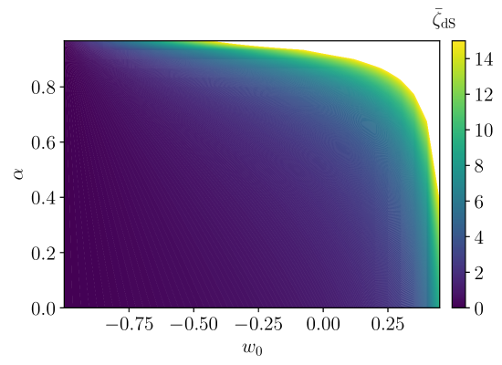
Figure 1: Behaviour of the maximum value of the bulk-viscosity coefficient $\bar{\zeta}_{\rm{dS}}$ as a function of the two free parameters in the model, $\alpha$ and $w_{0}$ [see Eq. (4.4)].

3 Numerical solutions

In this Section, we investigate the emergence of a quasi de-Sitter phase supported by bulk-viscosity pressure within a causal MIS formulation. To this scope, we solve numerically the generalized momentum conservation equation (2.1) and the effective EOS-parameter (2.17) under the quasi de-Sitter condition so as to obtain the evolution of the Hubble function. More specifically, substituting Eq. (2.45) in Eq. (LABEL:eq-15) gives

$$\left(\frac{\ddot{H}}{H^{3}}+3(w_{0}+1)\frac{\dot{H}}{H^{2}}\right)\left(\frac{2\alpha}{3}\frac{\dot{H}}{H^{2}}+(\alpha-1)(w_{0}+1)\right)+$$

$$+\,\frac{3}{2}(w_{0}^{2}-1)\left[\frac{\sqrt{3}}{\bar{\zeta}}\left(\sqrt{3}\alpha\bar{\zeta}+w_{0}+1\right)\left(\frac{2}{3}\frac{\dot{H}}{H^{2}}+w_{0}+1\right)-3(w_{0}+1)\right]+$$

$$\frac{9}{4(w_{0}+1)}\left(\frac{2}{3}\frac{\dot{H}}{H^{2}}+w_{0}+1\right)\left(w_{0}+1-\frac{2}{3}(2w_{0}+1)\frac{\dot{H}}{H^{2}}\right)\left(\frac{2\alpha}{3}\frac{\dot{H}}{H^{2}}+(\alpha-1)(w_{0}+1)\right)=0\,,$$

so that the Hubble function is determined by solving Eq. (3) numerically for given values of $\alpha$ and $w_{0}$, under the quasi de-Sitter condition that $-\dot{H}\ll H^{2}$. Note that because $w_{\mathrm{eff}}$ is a time-dependent function under the quasi de-Sitter condition, we express Eq. (3) in terms of a first-order ordinary differential equation in $w_{\mathrm{eff}}$ as follows

$$\frac{\dot{w}_{\rm eff}}{3H(t)}+\frac{(1+w_{0}+\sqrt{3}\,\alpha\,\bar{\zeta})(1-w_{0}^{2})(w_{\mathrm{{eff}}}-w_{0})}{\sqrt{3}\,\bar{\zeta}(1+w_{0}+\alpha(w_{\mathrm{eff}}-w_{0}))}+\frac{(1-w_{0}^{2})(1+w_{0})}{(1+w_{0}+\alpha(w_{\mathrm{eff}}-w_{0}))}-\frac{(w_{\mathrm{{eff}}}-w_{0})^{2}}{2(1+w_{0})}=0\,,$$

where we have made use of the fact that

$$H(t)=\frac{2}{3}\left[\int(1+w_{\mathrm{eff}}(t))dt\right]^{-1}\,.$$ (3.3)

The evolution of $w_{\rm{eff}}$ is determined by solving numerically Eq. (3), with initial condition $w_{\mathrm{eff}}(t_{\rm in})\approx-1$ (i.e., $w_{\mathrm{eff}}-1=10^{-12}$) as expected if the universe is nearly de-Sitter at $t=t_{\rm{in}}$ and possesses a nonzero bulk-viscosity pressure $\Pi(t_{\rm{in}})\sim 3H_{\rm in}^{2}(w_{\mathrm{eff}}(t_{\rm{in}})-w_{0})$, where $H_{\rm in}$ is the Hubble constant at $t=t_{\rm in}$.

Figure 2 shows the evolution of $H(t)$ under the quasi de-Sitter condition that $-\dot{H}\ll H^{2}$ for $\alpha=0.1$ and $w_{0}=-0.975$. Note that the Hubble function, which is initially set to take the value at which inflation is believed to have taken place, i.e., $H=10^{16}\,{\rm GeV}\approx 10^{-3}\,M_{\rm{pl}}$, remains essentially constant, but then it starts to slowly fall-off. During this period, as shown by Fig. 2, the first Hubble slow-roll parameter remains small and satisfies the condition $\epsilon_{\rm{H}}\ll 1$. The behaviour of $w_{\rm eff}$ is shown in the various panels of Fig. 3 for different values of the parameters $\bar{\zeta}$, $\alpha$ and $w_{0}$.

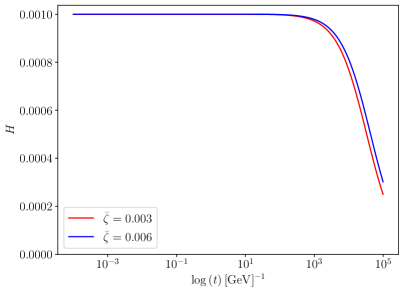
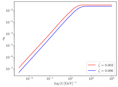
Figure 2: Left panel: Evolution of Hubble function $H(t)$ for for a representative choice of $\alpha=0.1$ and $w_{0}=-0.975$. Right panel: The same as in the left panel but for the slow-roll parameter (or first Hubble-flow) parameter.

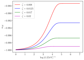
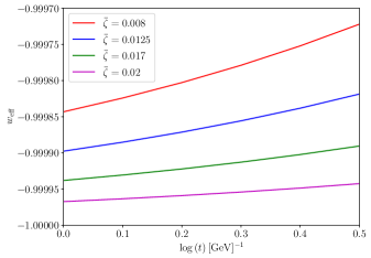
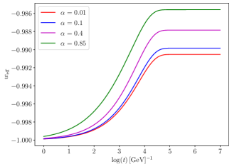
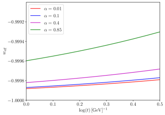
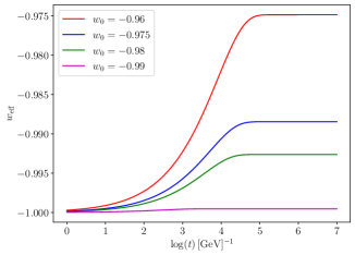
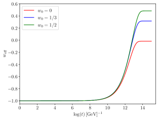
Figure 3: Top row: Evolution of $w_{\rm eff}$ for different values of $\bar{\zeta}$ for reference values of $\alpha=0.1$ and $w_{0}=-0.975$. The right panel simply shows a magnification of the early evolution. Middle row: the same as above but for different values of $\alpha$ while keeping fixed $w_{0}=-0.975$ and $\bar{\zeta}=0.01$. Bottom row: the same as above but for different values of $w_{0}$ while keeping fixed $\bar{\zeta}=0.01$ and $\alpha=0.3$.

In essence, all variations of the parameters show that, through the time-evolving bulk-viscosity pressure $\Pi(t)$, the effective EOS-parameter $w_{\mathrm{eff}}$ evolves time and finally attains a nearly constant value at a late time value during the quasi de-Sitter inflationary period. More specifically, the effect of varying $\bar{\zeta}$ on the effective EOS-parameter is shown in the top row of Fig. 3, where it is found $w_{\mathrm{eff}}$ departs from the exact de-Sitter value as $\bar{\zeta}$ is slowly decreased from its maximum value $\bar{\zeta}_{\rm dS}$ ($\bar{\zeta}_{\rm dS}=0.0214$ for $\alpha=0.1$ and $w_{0}=-0.975$). As a result, the more the magnitude of $\bar{\zeta}$ is decreased, the greater the departure from the exact de-Sitter evolution. Similarly, the influence of the variation of $\alpha$ on $w_{\mathrm{{eff}}}$ is presented in the middle row of Fig. 3, where it can be observed that as $\alpha$ is increased, $w_{\mathrm{{eff}}}$ deviates swiftly from the de-Sitter phase, implying that an increase of the non-equilibrium characteristic timescale $\tau_{*}$ leads to an increasing large departure from the exact de-Sitter state. Stated different, if non-equilibrium effects are present for a sufficiently long time, the universe cannot remain close to exact de-Sitter state. Finally, the bottom row of Fig. 3 reports the behaviour of $w_{\mathrm{eff}}$ due to variations of the parameter $w_{0}$ while keeping $\alpha$ and $\bar{\zeta}$ fixed. Since the value $w_{0}=-1$ is not allowed, decreasing $|w_{0}|$ leads to departures of $w_{\rm eff}$ from the exact de-Sitter phase for finite and positive values of $\bar{\zeta}$ and $\alpha$.

It is worth noting that the profile of $w_{\rm{eff}}$ is a feature which is purely a consequence of bulk-viscous effects subject to quasi de-Sitter conditions. In this regard, an insightful example is the evolution when $w_{0}=0$ (see bottom-right panel of Fig. 3). In this case, in fact, the evolution of $w_{\rm{eff}}$ depends only on $\bar{\zeta}$ and $\alpha$. The effective EOS-parameter exhibits a departure from the exact de-Sitter phase which is qualitatively very similar to the cases when $w_{0}\neq 0$. Furthermore, late-time value of $w_{\rm{eff}}$ increases systematically when decreasing $\bar{\zeta}$, it increases for larger values of $\alpha$ and $w_{0}$. Finally, we note that during the quasi de-Sitter expansion, the absolute magnitude of the bulk-viscosity pressure can be estimated using the quantity $|w_{\rm{eff}}-w_{0}|$, which is reported in Fig. 4. As in part to be expected, the bulk-viscosity pressure decreases, as $\bar{\zeta}$ decreases from $\bar{\zeta}_{\rm{dS}}$ and becomes zero in the limit in which $\bar{\zeta}\rightarrow 0$. All in all, the results presented in Fig. 3 clearly indicate that the effective EOS-parameter evolves following a unique functional behaviour, namely, from an almost constant and small initial value to an almost constant and large final value. However, the details on the transition between these two states is a function of the three parameters involved in the evolution: $\bar{\zeta},\alpha$, and $w_{0}$.

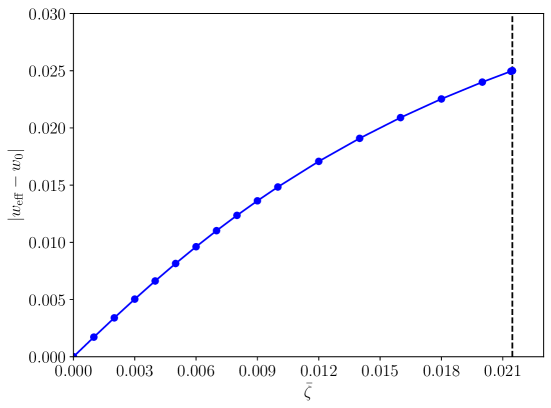
Figure 4: Variation of the absolute magnitude of the bulk-viscosity pressure $|w_{\rm{eff}}-w_{0}|$ as a function of the bulk-viscosity coefficient $\bar{\zeta}$ for reference values of $\alpha=0.1$ and $w_{0}=-0.975$; the vertical dotted line marks the maximum value $\bar{\zeta}_{\rm{dS}}=0.02147$.

4 Results and interpretation

In what follows we summarise the bulk of results obtained in our numerical investigation and provide a global interpretation of the various behaviours encountered. We start by considering what are the ranges in which the parameters of our approach, namely $w_{0}$, $\bar{\zeta}$, and $\alpha$, can vary.

4.1 Admissible regions of the parameters

We first note that we have restricted our study to values of the EOS-parameter such that $-1\leq w_{0}\leq 1$, so that we do not consider the case $w_{0}<-1$ for which the scenario of phantom inflation is often considered [48, 49, 50]. Clearly, using Eq. (3) with $w_{0}=-1$ yields $\dot{H}=0$, that is, the standard and non-viscous exact de-Sitter universe [note that in this case $\bar{\zeta}_{\rm dS}=0$, as expressed by Eq. (2.48)]. On the other hand, when $w_{0}=1$ Eq. (3) gives rise to $\dot{H}\neq 0$, so a quasi-de-Sitter phase can in principle exist in this limit provided the conditions $\dot{H}<0$ and $-{\dot{H}}/{H^{2}}\ll 1$ are valid. What remains problematic, however, is that in this case the relaxation timescale $\tau_{{}_{\Pi}}$ diverges; for this reason, we will not consider the value $w_{0}=1$ as admissible in our analysis. Another potentially problematic value for the EOS-parameter is $w_{0}=1/2$, which results into a diverging $\bar{\zeta}_{\rm{dS}}$ [42]; however so long as quasi de-Sitter conditions remain in place, i.e., $\dot{H}<0$ and $-{\dot{H}}/{H^{2}}\ll 1$, the issue of divergence of $\bar{\zeta}_{\rm{dS}}$ at $w_{0}={1}/{2}$ does not arise. This is shown in the bottom row of Fig. 3, where and observe that $w_{\mathrm{{eff}}}$ is finite and well-behaved over the entire interval $-1<w_{0}<1$ for different magnitudes of $\bar{\zeta}$.

Let us now consider the set of possible solutions starting from the inviscid limit ($\bar{\zeta}=0$), which leads to $w_{\mathrm{{eff}}}=w_{0}$ i.e., a constant effective EOS-parameter. Under these conditions, Eq. (3) reduces to

$$\frac{3\sqrt{3}}{2}(w_{0}^{2}-1)\left(1+w_{0}\right)\left(\frac{2}{3}\frac{\dot{H}}{H^{2}}+1+w_{0}\right)=0\,,$$ (4.1)

whose possible solutions are:

• $w_{0}=1$: this is the perfect-fluid cosmological solution with an ultra-stiff EOS [41].

• $w_{0}=-1$: this corresponds to the exact de-Sitter solution.

• $\displaystyle\frac{2}{3}\frac{\dot{H}}{H^{2}}+1+w_{0}=0$: the corresponding solution is given by

  $$H(t)=\frac{2}{3t(w_{0}+1)-2c_{1}}\,,$$ (4.2)

  where the integration constant may be chosen to be $c_{1}=0$ or $c_{1}<0$ to keep $H(t)$ finite. More specifically, if $c_{1}=0$, the scale-factor is then given by

  $$a(t)\propto[3t(1+w_{0})]^{2/3(w_{0}+1)}\,.$$ (4.3)

  Equations (4.2) and (4.3) thus provide straightforward expressions for the evolution of the Hubble parameter and of the scale-factor for either pressureless matter ($w_{0}=0$) or for radiation-dominated ($w_{0}={1}/{3}$) universe.

To determine the maximum allowed value of $\bar{\zeta}$, Eq. (3) is re-expressed in terms of $\epsilon_{\rm H}$ (which lies in the interval $0\leq\epsilon_{\rm H}\,\textless\,1$). Substituting $w_{\mathrm{eff}}=-1+(2/3)\epsilon_{\rm H}$ in Eq. (3) one arrives at

$$\frac{\dot{\epsilon}_{\rm H}}{3H(1-w_{0}^{2})}+\frac{(1+w_{0}+\sqrt{3}\alpha\bar{\zeta})(-1+\frac{2}{3}\epsilon_{\rm H}-w_{0})}{\sqrt{3}\bar{\zeta}[1+w_{0}+\alpha(-1+\frac{2}{3}\epsilon_{\rm H}-w_{0})]}+\frac{(1+w_{0})}{[1+w_{0}+\alpha(-1+\frac{2}{3}\epsilon_{\rm H}-w_{0})]}-$$

$$\frac{(1-\frac{2}{3}\epsilon_{\rm H}+w_{0})^{2}}{2(1+w_{0})(1-w_{0}^{2})}=0\,.$$

The maximum value of the bulk viscosity $\bar{\zeta}$ required for sustaining an accelerated expansion $\bar{\zeta}_{\rm{max}}$ is obtained when considering $\epsilon_{\rm H}=0$ and $\dot{\epsilon_{\rm H}}\approx 0$ and is found to be

$$\bar{\zeta}_{\rm{max}}=\frac{2\left(w_{0}^{2}-1\right)}{\sqrt{3}(1-\alpha)(2w_{0}-1)}=\bar{\zeta}_{\rm dS}\,,$$ (4.4)

which exactly matches with Eq. (2.48) and equals to the magnitude of the bulk viscosity that would give rise to an exact de-Sitter expansion.

As a consistency check, we can set $\bar{\zeta}=\bar{\zeta}_{\rm{max}}$ in Eq. (3) to obtain

$$(w_{\rm{eff}}+1)\left[w_{\rm{eff}}(-\alpha-3\alpha w_{0}+w_{0}+1)+\alpha w_{\rm{eff}}^{2}+(2\alpha+1)w_{0}^{2}+2w_{0}^{3}+(\alpha-3)w_{0}-2\right]=0\,,$$ (4.5)

which has three real roots one of which is $w_{\rm{eff}}=-1$. The other two roots are

$$w_{\rm{eff}}=\frac{-\alpha+(w_{0}+1)\sqrt{\alpha^{2}+\alpha(6-8w_{0})+1}-3\alpha w_{0}+w_{0}+1}{2\alpha}\,,$$ (4.6)

and

$$w_{\rm{eff}}=\frac{\alpha+(w_{0}+1)\sqrt{\alpha^{2}+\alpha(6-8w_{0})+1}+3\alpha w_{0}-w_{0}-1}{2\alpha}\,,$$ (4.7)

and are not relevant here, since for Eq. (4.6) $w_{\rm{eff}}<-1$ in the range $0<\alpha<1$, while for Eq. (4.7) $w_{\rm{eff}}>1$ in the range $-0.5<w_{0}<1$ and for all values of $\alpha$. As a result, $w_{\rm{eff}}=-1$ is the only possible solution of Eq. (3) during the exact de-Sitter phase when $\bar{\zeta}=\bar{\zeta}_{\rm{max}}$.

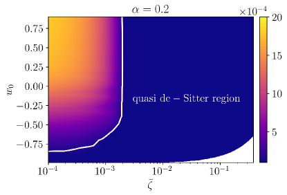
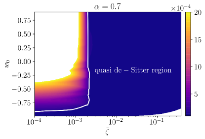
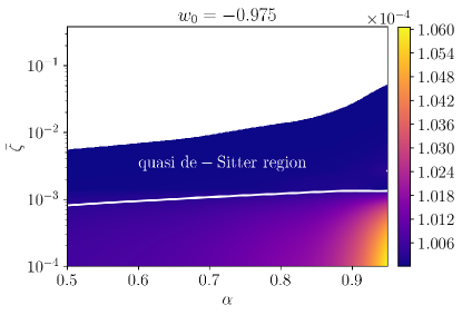
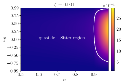
Figure 5: Colourmaps of the measure of the deviation from the quasi de-Sitter condition via the quantity $-\dot{H}/{H^{2}}$ ($-\dot{H}/{H^{2}}\ll 1$ corresponds to a quasi de-Sitter expansion and the white line marks the critical value $-\dot{H}/H^{2}=0.00016$. The maps are obtained by solving Eq. (3) for different magnitudes of the parameters $\bar{\zeta}$, $w_{0}$, and $\alpha$, with the first row referring to scenarios in which $\alpha=0.2$ (left) and $\alpha=0.7$ (right). The bottom row is the same as the top one but when considering constant values of $w_{0}=-0.975$ (left) and $\bar{\zeta}=0.001$ (right), respectively.

In order to represent the effects of the variations of $w_{0}$, $\bar{\zeta}$ and $\alpha$ on the solution obtained during the quasi de-Sitter inflationary period, we present in Fig. 5 and with colour maps the values of $-\dot{H}/H^{2}$ obtained when varying either $\bar{\zeta}$ or $\alpha$ while keeping one of these quantities fixed. In each case, we have considered the admissible ranges of the parameters $\alpha,\bar{\zeta}$ and $w_{0}$ and found that quasi de-Sitter solutions exist over the entire interval $-1<w_{0}<1$ of $w_{0}$. However, the top panels of Fig. 5 also show that significant deviations from the quasi de-Sitter evolutions can take place if $\bar{\zeta}$ is kept small. More specifically, while for large negative values of $w_{0}$ (i.e., $w_{0}\lesssim-0.81$) a de-Sitter evolution is possible even for large values of the bulk viscosity, as the EOS parameter increases, a substantial amount of bulk viscosity is necessary to ensure a de-Sitter evolution. In particular, setting as a critical value $-\dot{H}/H^{2}=0.00016$, we have found the a de-Sitter evolution is possible only for $\bar{\zeta}\gtrsim 10^{-4}$ (see left panel of Fig. 5). Interestingly, for $w_{0}\gtrsim-0.25$ the amount of bulk viscosity needed to ensure a de-Sitter evolution is essentially constant a corresponds to $\bar{\zeta}\sim 2\times 10^{-3}$. Stated differently, while a quasi de-Sitter evolution is possible for any value of $w_{0}$ if the bulk viscosity is large, the latter is small only a delicate balance is required between $w_{0}$ and $\bar{\zeta}$. Note also that the considerations made above depend – although not sensitively – on the value of $\alpha$, as can be appreciated when comparing the left and right top panels of Fig. 5. More specifically, the regions of quasi de-Sitter evolution tends to be slightly reduced as $\alpha$ is increased.

The lower-left panel of Fig. 5, on the other hand, shows that the impact of the $\alpha$ parameter is small so long as $w_{0}\sim-1$ and the deviation from the quasi de-Sitter phase remains small over the entire range of $\alpha$. For instance, a slight deviation from quasi de-Sitter phase takes place only for very small values of the bulk-viscosity coefficient around $\bar{\zeta}\lesssim 10^{-3}$, with the deviation becoming comparatively larger as $\alpha$ becomes close to unity. However, for bulk viscosities $\bar{\zeta}\gtrsim 10^{-3}$, a quasi de-Sitter phase always SL: exists independently of the value of $\alpha$. Finally, the lower-right panel of Fig. 5 reports the deviation from exact de-Sitter when considering a fixed bulk-viscosity coefficient $\bar{\zeta}=0.001$ and varying the two coefficients $w_{0}$ and $\alpha$. In this case, it is clear that the quasi de-Sitter expansion takes place for all values $w_{0}$ so long as $\alpha\lesssim 0.9$. However, when $\alpha\gtrsim 0.9$, deviations from de-Sitter become large for most of the range of $w_{0}$ and in particular if $w_{0}\geq-0.75$.

Given that $w_{\rm{eff}}$ does not remain constant during the quasi de-Sitter inflation but increases till reaching a new stationary value (see Fig. 3), it is reasonable to define a timescale $\tau$ that characterises how rapid the transition is from the exact de-Sitter phase to the new quasi de-Sitter inflation. We use the behaviour shown in Fig. 3 to express the evolution of $w_{\mathrm{eff}}$ as

$$\tilde{w}_{\mathrm{eff}}(x)=-1+\frac{A}{1+Be^{-x/\tau}}\,,$$ (4.8)

where $x:=\log_{10}t$ and the dimensionless constants $A,B$ depend on the bulk viscosity. Using a best-fit approach and the numerical results presented in Fig. 3 it is possible to compute both $\tau$ and $A,B$. Unsurprisingly, and just like $w_{\mathrm{eff}}$, also $\tau$ depends on $\bar{\zeta}$, $\alpha$, and $w_{0}$, so that, for $\alpha$ and $w_{0}$ fixed, $\tau$ simply decreases as $\bar{\zeta}$ is increased up to $\bar{\zeta}_{\rm{dS}}$. Indeed, for $w_{0}\rightarrow-1$, a considerable time is needed for $w_{\mathrm{eff}}$ to deviate from exact the de-Sitter phase (see the bottom-left panel in Fig. 3). This behaviour of $w_{\mathrm{eff}}$ is reflected on $\tau$ as well, which increases only very slowly even if $\bar{\zeta}\ll\bar{\zeta}_{\rm{dS}}$.

4.2 Estimation of the model parameters

We next turn our attention on estimating allowed values of these parameters by using constraints from primordial power spectrum generated by curvature perturbations during the inflationary period. Such an analysis will not only enable us to estimate realistic values of the bulk-viscosity coefficient and characteristic timescales, but will also allow us to examine the observational viability of quasi de-Sitter model of inflation supported by bulk viscosity. A straightforward procedure in this direction involves the evaluation of the inflationary variables, e.g., the spectral index of scalar curvature perturbations $n_{s}$ and the tensor-to-scalar ratio $r$, in terms of the model parameters $\bar{\zeta}$, $\alpha$ and $w_{0}$, and the comparison with the experimentally observed values of $n_{s}$ and $r$ obtained from the Planck data/WMAP data. A possible way to do this is to construct the fluid description of inflation in the context of the generalised causal theory following the procedure suggested by Bamba and Odintsov [51], who introduced an EOS which included bulk viscosity but did not consider a causal theory of hydrodynamics.

Typically, the inflationary variables are expressed in terms of slow-roll parameters which are in turn are represented in terms of potential of a scalar field driving inflation and their respective derivatives. The equivalence between the fluid description of inflation and the scalar-field description of inflation can be established provided the EOS of the bulk viscous fluid and that of the equation of the state followed by pressure and energy density of a scalar field are the same [51]. Hence, we will first elucidate the equivalence between the two descriptions.

We recall that the Friedmann equations when expressed in terms of the e-folding number $N$ are given by

$$3(H(N))^{2} = e(N)\,,$$ (4.9)

$$2H(N)H^{\prime}(N)+3(H(N))^{2} = -p_{\mathrm{eff}}(N)\,,$$ (4.10)

where $N$ is defined as $N:=\int^{t_{f}}_{t_{i}}Hdt$, so that the Hubble function becomes $H=H(N)$. Here, $t_{i}$ and $t_{f}$ are respectively the times corresponding to the beginning and end of inflation, while the index ^′ is used to indicate the derivative with respect to $N$. From Eq. (4.9) and Eq. (4.10), we then obtain

$$\frac{1}{2}\left[e(N)-p_{\mathrm{{eff}}}(N)\right]=H^{\prime}(N)H(N)+3(H(N))^{2}\,.$$ (4.11)

On the other hand, in the single scalar-field description of inflation, the action is given by

$$S:=\int d^{4}x\left(\frac{R}{2}-\frac{1}{2}\partial_{\mu}\phi\partial^{\mu}\phi-V(\phi)\right)\,,$$ (4.12)

where $\phi=\phi(t)$ is also known as the inflaton field and $V(\phi)$ is the inflaton potential. The components of Einstein equations are

$$3H^{2} = \frac{1}{2}\dot{\phi}^{2}+V(\phi)=e_{\phi}\,,$$ (4.13)

$$-(2\dot{H}+3H^{2}) = \frac{1}{2}\dot{\phi}^{2}-V(\phi)=p_{\phi}\,,$$ (4.14)

where $e_{\phi}$ and $p_{\phi}$ are the energy density and the pressure of the scalar field, respectively. Combining these two equations one obtains that

$$\dot{\phi}^{2}=-2\dot{H}\,.$$ (4.15)

The equivalence between two descriptions of inflation is obtained once the scalar field $\phi$ and the cosmological time $t$ are both rescaled by an auxiliary scalar field $\Phi$, thus implying $\phi=\phi(\Phi)$ and $t=t(\Phi)$, and when $\Phi$ identified with the e-folding number $N$. Under these conditions, Eq. (4.13) and Eq. (4.14) can be rewritten as,

$$3H^{2}(N) = \frac{1}{2}H^{2}(N)\left(\frac{d\phi}{d\Phi}\right)^{2}\Bigg{|}_{\Phi=N}+V(\phi(\Phi))|_{\Phi=N}\,,$$ (4.16)

$$-2H(N)H^{\prime}(N) = \frac{1}{2}H^{2}(N)\left(\frac{d\phi}{d\Phi}\right)^{2}\Bigg{|}_{\Phi=N}-V(\phi(\Phi))|_{\Phi=N}\,.$$ (4.17)

Using Eqs. (4.13)–(4.17), the scalar-field potential is given by

$$V(N) = H^{\prime}(N)H(N)+3H^{2}(N)=\frac{1}{2}(e_{\phi}-p_{\phi})\,.$$ (4.18)

Since the bulk viscous fluid and the scalar field possess the same EOS, together with Eq. (4.11) the potential can be expressed as

$$V(N) = H^{\prime}(N)H(N)+3H^{2}(N)=\frac{1}{2}\left[e(N)-p_{\mathrm{eff}}(N)\right]\,.$$ (4.19)

and Eq. (3) can be re-written in the following way in terms of $N$, namely,

$$\tau_{{}_{\Pi}}\frac{d\Pi(N)}{dN}\left(1+k^{2}\frac{\tau_{{}_{\Pi}}(N)}{\zeta(N)}\right)+\frac{\Pi(N)}{H(N)}\left(1+3k^{2}H(N)\tau_{{}_{\Pi}}\right)$$

$$=-3\zeta(N)-\frac{1}{2}\tau_{{}_{\Pi}}\Pi(N)\left[3+\frac{1}{\tau_{{}_{\Pi}}}\frac{d\tau_{{}_{\Pi}}}{dN}-\frac{1}{\zeta}\frac{d\zeta}{dN}-\frac{1}{T}\frac{dT}{dN}\right]\left(1+k^{2}\frac{\tau_{{}_{\Pi}}(N)}{\zeta(N)}\right)\,,$$ (4.20)

where the bulk viscosity is expressed as

$$\Pi(N) = -2H^{\prime}(N)H(N)+3(1+w_{0})H^{2}(N)\,.$$ (4.21)

Similarly, the relaxation time coefficient, the temperature and the bulk viscosity can also be expressed in terms of the e-folding number. Using the potential, it is then possible to determine the slow-roll parameters $\epsilon_{\rm V}(N)$ and $\eta_{\rm V}(N)$ purely in terms of $H(N)$, $H^{\prime}(N)$ and $H^{\prime\prime}(N)$ as [52]

$$\epsilon_{\rm V}(N)=-\frac{H}{4H^{\prime}}\left[\frac{6{H^{\prime}}/{H}+{H^{\prime\prime}}/{H}+\left({H^{\prime}}/{H}\right)^{2}}{3+{H^{\prime}}/{H}}\right]^{2}\,,$$ (4.22)

and

$$\eta_{\rm V}(N)=-\frac{1}{2}\left[\frac{9{H^{\prime}}/{H}+3{H^{\prime\prime}}/{H}+\frac{1}{2}\left({H^{\prime}}/{H}\right)^{2}-\frac{1}{2}\left({H^{\prime\prime}}/{H^{\prime}}\right)^{2}+3\left({H^{\prime\prime}}/{H^{\prime}}\right)+{H^{\prime\prime\prime}}/{H^{\prime}}\,}{\left(3+{H^{\prime}}/{H}\right)}\right]\,.$$ (4.23)

Typically, the energy scale of inflation and the e-folding number are respectively taken to be $H_{in}\simeq 10^{-3}$ $M_{\rm{Pl}}$ and $N\simeq 50$. Since we have set $\kappa=M_{\rm Pl}=1$, the energy scale of inflation becomes $H_{in}=10^{-3}$. Solving Eq. (4.20) numerically under the condition that $-H^{\prime}(N)\ll H(N)$ (or, equivalently, that $\dot{\phi}^{2}\ll V$ in a scalar-field description), we have found that $\epsilon_{\rm V}(N)$ and $\eta_{\rm V}(N)$ remain constant and smaller than unity when $N$ is taken to vary in the interval $N\in[0,50]$ and $\alpha,w_{0}$ and $\bar{\zeta}$ are varied appropriately (see discussion in Sec. 4.3). This suggests that slow-roll conditions are indeed obeyed during quasi de-Sitter inflationary phase described by a generalised causal theory. Consequently, the inflationary observables $n_{s}$ and $r$ that characterise the perturbation spectra can then be related to the potential slow-roll parameters $\epsilon_{\rm V}(N)$ and $\eta_{\rm V}(N)$ as follows (see, e.g., , [53])

$$n_{s} = 1-6\epsilon_{\rm V}+2\eta_{\rm V}\,,$$ (4.24)

$$r = 16\epsilon_{\rm V}\,.$$ (4.25)

We note that while for exact de-Sitter expansion one should have $n_{s}=1$ and $r=0$, observations from Cosmic Microwave Background (CMB) strongly suggest small but non-zero deviation of $n_{s}$, thus suggesting a scale dependence of the density fluctuations and indicating a nearly de-Sitter expansion, and a small but nonzero value for $r$.

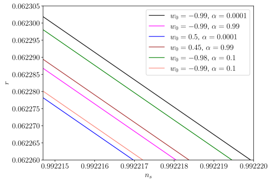
Figure 6: Behaviour of the spectral index $n_{s}$ and of the tensor-to-scalar ratio $r$ as predicted by our model. These quantities are evaluated using Eqs. (4.24)–(4.25) for different values of $w_{0}$, $\alpha$ and $\bar{\zeta}$ when they are varied within the corresponding allowed ranges.

The behaviour of $n_{s}$ and $r$ as predicted by our model is illustrated in Fig. 6, where we evaluated these quantities using Eqs. (4.24) and (4.25) for different values of $w_{0}$, $\alpha$ and $\bar{\zeta}$ when they are varied within the corresponding allowed ranges. Note that the results show an essentially linear behaviour and that each point of a specific line corresponds to a unique value of $\bar{\zeta}$ for fixed values of $\alpha$ and $w_{0}$, increasing from left to right as $n_{s}$ is increased. Note also that while each individual line represents a unique solution for fixed values of $\alpha$ and $w_{0}$, the actual variations in the spectral index are rather small and this explains the expanded scale shown in Fig. 6. In turn, this implies that the effective space of allowed values for $n_{s}$ and $r$ is essentially one-dimensional in our model, and that in the limit $n_{s}\to 1$, the tensor-to-scalar ratio is also vanishingly small, i.e., $r\to 0$.

4.3 Comparison with observations

In order to examine the compatibility of our model with current observational data, we consider three datasets obtained on observations from the Planck satellite and from other, non-Planck based observations. More specifically, we consider the observational constraints on $n_{s}$ and $r$ based on the Planck2018$+$ Keck-Array BK15 (hereafter “Planck$+$BK15”) data sets [54, 55, 56, 57], from the Atacama Cosmology Telescope DR4 likelihood combined with the WMAP satellite data set (hereafter “ACTPol$+$WMAP”) [58, 59], and from the South-Pole Telescope polarization measurements (hereafter “SPT3G$+$WMAP”) [58, 60]. The comparison of our model with these three observational datasets is carried out by considering two reference viscous-cosmology datasets, namely, $w_{0}=-0.98,\alpha=0.1$ and $w_{0}=-0.99,\alpha=0.1$, which are is shown in the three panels of Fig. 7 (given the small variance they appear as solid straight lines in the panels). Also reported are the constraints from the various datasets, namely, ACTPol$+$WMAP, SPT3G$+$WMAP, and Planck$+$BK15, from left to right. The comparison in Fig. 7 shows that the proposed model of inflation is clearly compatible with both the ACTPol$+$WMAP and the SPT3G$+$WMAP results, since the straight lines generated by the two reference viscous-cosmology datasets pass through the shaded regions in the $(n_{s},r)$ plane.

Furthermore, we note that when $w_{0}\rightarrow-1$, it is possible (and straightforward) to select values of $\bar{\zeta}$ and $\alpha$ within their allowed ranges of variation such that $n_{s}$ and $r$ match the observational constraints. On the other hand, when $w_{0}>0$, the bulk-viscosity coefficient needed is very large (typically ${\mathcal{O}}(1)-{\mathcal{O}}(10)$) in order to produce compatible values of $n_{s}$ and $r$. Note also that since Fig. 7 shows that the observations from ACTPol$+$WMAP predict a lower value of $r$ when compared to the the SPT3G$+$WMAP data, the magnitude of the bulk-viscosity coefficient required to produce compatible values of $n_{s}$ and $r$ will be different for the observational datasets. For instance, with $w_{0}=-0.98,\alpha=0.1$, a bulk viscosity coefficient $\bar{\zeta}\sim 7\times 10^{-3}$ ($\bar{\zeta}\sim 6\times 10^{-3}$) is necessary to produce values of $n_{s}$ and $r$ compatible with the constraints from the ACTPol$+$WMAP (SPT3G$+$WMAP) observations.

Finally, it should be remarked that although our model is supported by the ACTPol$+$WMAP and SPT3G$+$WMAP results, it is incompatible with the current Planck$+$BK15 datasets (third panel of Fig. 7) for all the values of $\alpha$ and $w_{0}$ that are allowed. In particular, the Planck$+$BK15 observations seem to predict values of the that is systematically smaller than the one obtained in our model for all of values that the spectral index is allowed to take.

It is worthwhile to note that our results are indeed in agreement with those presented in Refs. [61, 62], where a higher value of $n_{s}$ was also found and thus in accord with the constraints from ACTPol$+$WMAP and SPT3G$+$WMAP. In this sense, unless the differences are due to yet undetected systematic differences among the observations, the bulk viscosity model of inflation suggests a possible and slight modification of $\Lambda$CDM model scenario [63]. On the other hand, the discrepancy in the value of $n_{s}$ may also be related to the simplified phenomenological model adopted in this work for incorporating out-of-equilibrium effects during inflationary period of the early universe. The inclusion of non-equilibrium effects when gradients are large, as done for example in [64], may reduce the discrepancy with Planck$+$BK15 data and we will address this possibility in future work.

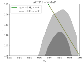
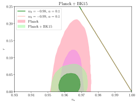
Figure 7: Comparison of bulk-viscous model of inflation (straight lines) with the marginalised contours of Planck$+$BK15, ACTPol$+$WMAP and SPT3G$+$WMAP results. The contours are obtained for $n_{s}$, $r$ using marginalised joint 68$\%$ and 95$\%$ confidence-level regions from the observational data.

5 Conclusions and outlook

There is a widespread consensus that the early universe has undergone a phase of quasi de-Sitter expansion and this is normally modelled by means of a suitable scalar field and of an associated potential. We have presented an alternative modelling of the inflationary expansion that is not based on a scalar field but that involves instead a bulk-viscous cosmological fluid to sustain a quasi de-Sitter expansion in the early universe. Our model is set in the framework of the generalised causal theory of hydrodynamics and by taking into account out-of-equilibrium effects, it reveals that, if the cosmological fluid possessed a nonzero bulk viscosity, then a quasi de-Sitter inflation arises naturally in this scenario without invoking to additional fields and without assuming an EOS of the type $p=w_{0}\,e=-e$ relating the equilibrium pressure and the energy density. Hence, a quasi de-Sitter inflation can be realised purely with the help of bulk-viscosity and by taking into consideration non-equilibrium effects that inevitably arise due to the violation of the SEC during the accelerated expansion of the early universe.

The model of inflation presented here has several interesting features. First, while the bulk viscosity provides the necessary negative pressure required for the accelerated expansion, as a matter of course, the effective EOS – expressed in term of the ratio between the effective pressure and the energy density, $w_{\mathrm{eff}}$ and that embodies the bulk-viscous and non-equilibrium effects – becomes a time-dependent function describing the time evolution of inflationary phase. Second, the evolution of $w_{\mathrm{eff}}$ follows a rather simple and unique behaviour that reflects a smooth transition from the exact de-Sitter phase and to a subsequent levelling-off to a constant value at later times. While this behaviour is obtained by solving numerically the generalized momentum-conservation equation, the functional behaviour of $w_{\mathrm{eff}}$ can be assimilated to a simple Logistic function and hence, the associated timescale for the transition from exact de-Sitter to the new quasi de-Sitter phase, be estimated accurately. This timescale is a simple function of the three parameters of the systems ($\bar{\zeta}$, $\alpha$ and $w_{0}$) and, unsurprisingly, it decreases as the magnitude of the bulk viscosity coefficient is increased up to the exact de-Sitter value. Third, in contrast to the standard inflationary scenario where $-1<w_{0}<1/2$, our bulk-viscous model allows for a larger range of values, namely, $-1<w_{0}<1$ and is well-behaved for $w_{0}=0$. Finally, the equivalence between the non-perfect fluid description of inflation presented here with the scalar-field theory of inflation is maintained also when considering the observational constraints. In particular, when expressing the constraints coming from Planck2018 [13], Keck-Array BK15, ACTPol+WMAP, and SPT3G+WMAP [61], in terms of the standard inflationary variables like the spectral index of scalar density perturbations $n_{s}$ and tensor-to-scalar ratio $r$. We find that these constraints can be easily satisfied by suitable choices of $\bar{\zeta}$, $\alpha$, and $w_{0}$ for the ACTPol$+$WMAP and SPT3G$+$WMAP datasets, while tensions appear in the case of the Planck$+$BK15 datasets.

The work presented here can be extended and improved in a number of directions. For example, by investigating the possible origin of bulk viscosity in the early universe and relating it to the mechanism of particle production [26]. Similarly, it would be interesting to investigate the precise mechanism gives rise to the exit from the quasi de-Sitter inflationary phase and could lead to conducive conditions for reheating. Finally, the study of warm inflation recently suggested in Ref. [65] could also be re-analysed when framed in the presence of bulk viscosity and non-equilibrium effects. We leave all of these investigations to future works.

References

- [1] A. H. Guth, “Inflationary universe: A possible solution to the horizon and flatness problems,” Phys. Rev. D, vol. 23, pp. 347–356, Jan 1981.
- [2] A. D. Linde, “A New Inflationary Universe Scenario: A Possible Solution of the Horizon, Flatness, Homogeneity, Isotropy and Primordial Monopole Problems,” Phys. Lett. B, vol. 108, pp. 389–393, 1982.
- [3] A. A. Starobinsky, “A new type of isotropic cosmological models without singularity,” Physics Letters B, vol. 91, pp. 99–102, Mar. 1980.
- [4] V. F. Mukhanov and G. V. Chibisov, “Quantum Fluctuations and a Nonsingular Universe,” JETP Lett., vol. 33, pp. 532–535, 1981.
- [5] S. W. Hawking, “The development of irregularities in a single bubble inflationary universe,” Physics Letters B, vol. 115, pp. 295–297, 1982.
- [6] A. H. Guth and S.-Y. Pi, “Fluctuations in the new inflationary universe,” Phys. Rev. Lett., vol. 49, pp. 1110–1113, Oct 1982.
- [7] P. A. R. Ade, R. W. Aikin, D. Barkats, S. J. Benton, C. A. Bischoff, J. J. Bock, J. A. Brevik, I. Buder, E. Bullock, C. D. Dowell, L. Duband, J. P. Filippini, S. Fliescher, S. R. Golwala, M. Halpern, M. Hasselfield, S. R. Hildebrandt, G. C. Hilton, V. V. Hristov, K. D. Irwin, K. S. Karkare, J. P. Kaufman, B. G. Keating, S. A. Kernasovskiy, J. M. Kovac, C. L. Kuo, E. M. Leitch, M. Lueker, P. Mason, C. B. Netterfield, H. T. Nguyen, R. O’Brient, R. W. Ogburn, A. Orlando, C. Pryke, C. D. Reintsema, S. Richter, R. Schwarz, C. D. Sheehy, Z. K. Staniszewski, R. V. Sudiwala, G. P. Teply, J. E. Tolan, A. D. Turner, A. G. Vieregg, C. L. Wong, and K. W. Yoon, “Detection of -mode polarization at degree angular scales by bicep2,” Phys. Rev. Lett., vol. 112, p. 241101, Jun 2014.
- [8] E. Ayón-Beato and A. García, “Regular Black Hole in General Relativity Coupled to Nonlinear Electrodynamics,” Physical Review Letters, vol. 80, pp. 5056–5059, 1998.
- [9] D. N. Spergel, L. Verde, H. V. Peiris, E. Komatsu, M. R. Nolta, C. L. Bennett, M. Halpern, G. Hinshaw, N. Jarosik, A. Kogut, M. Limon, S. S. Meyer, L. Page, G. S. Tucker, J. L. Weiland, E. Wollack, and E. L. Wright, “First-Year Wilkinson Microwave Anisotropy Probe (WMAP) Observations: Determination of Cosmological Parameters,” Astrophys. J., Supp., vol. 148, pp. 175–194, Sept. 2003.
- [10] D. N. Spergel, R. Bean, O. Doré, M. R. Nolta, C. L. Bennett, J. Dunkley, G. Hinshaw, N. Jarosik, E. Komatsu, L. Page, H. V. Peiris, L. Verde, M. Halpern, R. S. Hill, A. Kogut, M. Limon, S. S. Meyer, N. Odegard, G. S. Tucker, J. L. Weiland, E. Wollack, and E. L. Wright, “Three-Year Wilkinson Microwave Anisotropy Probe (WMAP) Observations: Implications for Cosmology,” Astrophys. J., Supp., vol. 170, pp. 377–408, June 2007.
- [11] E. Komatsu, K. M. Smith, J. Dunkley, C. L. Bennett, B. Gold, G. Hinshaw, N. Jarosik, D. Larson, M. R. Nolta, L. Page, D. N. Spergel, M. Halpern, R. S. Hill, A. Kogut, M. Limon, S. S. Meyer, N. Odegard, G. S. Tucker, J. L. Weiland, E. Wollack, and E. L. Wright, “Seven-year Wilkinson Microwave Anisotropy Probe (WMAP) Observations: Cosmological Interpretation,” Astrophys. J., Supp., vol. 192, p. 18, Feb. 2011.
- [12] P. A. R. Ade et al., “Planck 2013 results. XXII. Constraints on inflation,” Astron. Astrophys., vol. 571, p. A22, 2014.
- [13] Y. Akrami, F. Arroja, M. Ashdown, J. Aumont, C. Baccigalupi, M. Ballardini, A. J. Banday, R. Barreiro, N. Bartolo, S. Basak, et al., “Planck 2018 results-x. constraints on inflation,” Astronomy & Astrophysics, vol. 641, p. A10, 2020.
- [14] A. D. Linde, “Chaotic Inflation,” Phys. Lett. B, vol. 129, pp. 177–181, 1983.
- [15] D. Baumann, “Inflation,” in Theoretical Advanced Study Institute in Elementary Particle Physics: Physics of the Large and the Small, pp. 523–686, 2011.
- [16] F. Bezrukov and M. Shaposhnikov, “The standard model higgs boson as the inflaton,” Physics Letters B, vol. 659, no. 3, pp. 703–706, 2008.
- [17] K. Freese, J. A. Frieman, and A. V. Olinto, “Natural inflation with pseudo nambu-goldstone bosons,” Phys. Rev. Lett., vol. 65, pp. 3233–3236, Dec 1990.
- [18] B. A. Bassett, S. Tsujikawa, and D. Wands, “Inflation dynamics and reheating,” Rev. Mod. Phys., vol. 78, pp. 537–589, 2006.
- [19] D. Wands, “Multiple field inflation,” Lect. Notes Phys., vol. 738, pp. 275–304, 2008.
- [20] S. Kachru, R. Kallosh, A. D. Linde, J. M. Maldacena, L. P. McAllister, and S. P. Trivedi, “Towards inflation in string theory,” JCAP, vol. 10, p. 013, 2003.
- [21] G. R. Dvali and S. H. H. Tye, “Brane inflation,” Phys. Lett. B, vol. 450, pp. 72–82, 1999.
- [22] A. A. Starobinsky, “A New Type of Isotropic Cosmological Models Without Singularity,” Phys. Lett. B, vol. 91, pp. 99–102, 1980.
- [23] P. Kanti, R. Gannouji, and N. Dadhich, “Gauss-Bonnet Inflation,” Phys. Rev. D, vol. 92, no. 4, p. 041302, 2015.
- [24] T. Clifton, P. G. Ferreira, A. Padilla, and C. Skordis, “Modified Gravity and Cosmology,” Phys. Rept., vol. 513, pp. 1–189, 2012.
- [25] R. Maartens, “Dissipative cosmology,” Classical and Quantum Gravity, vol. 12, no. 6, p. 1455, 1995.
- [26] W. Zimdahl, “Bulk viscous cosmology,” Phys. Rev. D, vol. 53, pp. 5483–5493, May 1996.
- [27] I. Brevik and O. Gorbunova, “Dark energy and viscous cosmology,” General Relativity and Gravitation, vol. 37, no. 12, pp. 2039–2045, 2005.
- [28] J. A. Belinchón, O. Cornejo-Pérez, and N. Cruz, “Exact solutions of a causal viscous FRW cosmology within the Israel–Stewart theory through factorization,” Gen. Rel. Grav., vol. 54, no. 1, p. 10, 2022.
- [29] E. A. Hakk, A. N. Tawfik, A. Nada, and H. Yassin, “Cosmic Evolution of Viscous QCD Epoch in Causal Eckart Frame,” Universe, vol. 7, no. 5, p. 112, 2021.
- [30] I. Brevik and A. V. Timoshkin, “Thermodynamic aspects of entropic cosmology with viscosity,” Int. J. Mod. Phys. D, vol. 30, no. 02, p. 2150008, 2021.
- [31] V. H. Cárdenas, M. Cruz, and S. Lepe, “Cosmic expansion with matter creation and bulk viscosity,” Phys. Rev. D, vol. 102, no. 12, p. 123543, 2020.
- [32] W. Yang, S. Pan, E. Di Valentino, A. Paliathanasis, and J. Lu, “Challenging bulk viscous unified scenarios with cosmological observations,” Phys. Rev. D, vol. 100, no. 10, p. 103518, 2019.
- [33] N. Cruz, E. González, and G. Palma, “Exact analytical solution for an Israel–Stewart cosmology,” Gen. Rel. Grav., vol. 52, no. 6, p. 62, 2020.
- [34] I. Brevik, E. Elizalde, S. D. Odintsov, and A. V. Timoshkin, “Inflationary universe in terms of a van der Waals viscous fluid,” Int. J. Geom. Meth. Mod. Phys., vol. 14, no. 12, p. 1750185, 2017.
- [35] I. Brevik, O. Grøn, J. de Haro, S. D. Odintsov, and E. N. Saridakis, “Viscous Cosmology for Early- and Late-Time Universe,” Int. J. Mod. Phys. D, vol. 26, no. 14, p. 1730024, 2017.
- [36] I. Muller, “Zum Paradoxon der Warmeleitungstheorie,” Z. Phys., vol. 198, pp. 329–344, 1967.
- [37] W. Israel, “Nonstationary irreversible thermodynamics: a causal relativistic theory,” Annals of Physics, vol. 100, no. 1-2, pp. 310–331, 1976.
- [38] W. Israel, “Thermo-field dynamics of black holes,” Physics Letters A, vol. 57, no. 2, pp. 107–110, 1976.
- [39] W. A. Hiscock and L. Lindblom, “Generic instabilities in first-order dissipative relativistic fluid theories,” Physical Review D, vol. 31, no. 4, p. 725, 1985.
- [40] W. A. Hiscock and L. Lindblom, “Stability and causality in dissipative relativistic fluids,” Annals of Physics, vol. 151, no. 2, pp. 466–496, 1983.
- [41] L. Rezzolla and O. Zanotti, Relativistic Hydrodynamics. Oxford, UK: Oxford University Press, 2013.
- [42] R. Maartens and V. Mendez, “Nonlinear bulk viscosity and inflation,” Physical Review D, vol. 55, no. 4, p. 1937, 1997.
- [43] R. Maartens, M. Govender, and S. D. Maharaj, “Inflation driven by causal heat flux,” Gen. Rel. Grav., vol. 31, pp. 815–819, 1999.
- [44] M. Chabanov, L. Rezzolla, and D. H. Rischke, “General-relativistic hydrodynamics of non-perfect fluids: 3+1 conservative formulation and application to viscous black hole accretion,” Monthly Notices of the Royal Astronomical Society, vol. 505, pp. 5910–5940, Aug. 2021.
- [45] F. S. Bemfica, M. M. Disconzi, and J. Noronha, “Causality of the Einstein-Israel-Stewart Theory with Bulk Viscosity,” Phys. Rev. Lett., vol. 122, no. 22, p. 221602, 2019.
- [46] P. Kovtun, “First-order relativistic hydrodynamics is stable,” JHEP, vol. 10, p. 034, 2019.
- [47] R. Maartens, “Causal Thermodynamics in Relativity,” arXiv e-prints, pp. astro–ph/9609119, Sept. 1996.
- [48] S. Capozziello, S. Nojiri, and S. D. Odintsov, “Unified phantom cosmology: Inflation, dark energy and dark matter under the same standard,” Phys. Lett. B, vol. 632, pp. 597–604, 2006.
- [49] E. N. Saridakis, “Theoretical Limits on the Equation-of-State Parameter of Phantom Cosmology,” Phys. Lett. B, vol. 676, pp. 7–11, 2009.
- [50] M. Khurshudyan, “On the Phenomenology of an Accelerated Large-Scale Universe,” Symmetry, vol. 8, no. 12, p. 110, 2016.
- [51] K. Bamba and S. D. Odintsov, “Inflation in a viscous fluid model,” The European Physical Journal C, vol. 76, no. 1, pp. 1–12, 2016.
- [52] K. Bamba, S. Nojiri, and S. D. Odintsov, “Reconstruction of scalar field theories realizing inflation consistent with the Planck and BICEP2 results,” Phys. Lett. B, vol. 737, pp. 374–378, 2014.
- [53] A. Riotto, “Inflation and the theory of cosmological perturbations,” ICTP Lect. Notes Ser., vol. 14, pp. 317–413, 2003.
- [54] N. Aghanim et al., “Planck 2018 results. V. CMB power spectra and likelihoods,” Astron. Astrophys., vol. 641, p. A5, 2020.
- [55] N. Aghanim et al., “Planck 2018 results. VI. Cosmological parameters,” Astron. Astrophys., vol. 641, p. A6, 2020. [Erratum: Astron.Astrophys. 652, C4 (2021)].
- [56] N. Aghanim et al., “Planck 2018 results. I. Overview and the cosmological legacy of Planck,” Astron. Astrophys., vol. 641, p. A1, 2020.
- [57] P. A. R. Ade et al., “BICEP2 / Keck Array x: Constraints on Primordial Gravitational Waves using Planck, WMAP, and New BICEP2/Keck Observations through the 2015 Season,” Phys. Rev. Lett., vol. 121, p. 221301, 2018.
- [58] G. Hinshaw, D. Larson, E. Komatsu, D. N. Spergel, C. L. Bennett, J. Dunkley, M. R. Nolta, M. Halpern, R. S. Hill, N. Odegard, L. Page, K. M. Smith, J. L. Weiland, B. Gold, N. Jarosik, A. Kogut, M. Limon, S. S. Meyer, G. S. Tucker, E. Wollack, and E. L. Wright, “Nine-year Wilkinson Microwave Anisotropy Probe (WMAP) Observations: Cosmological Parameter Results,” apjs, vol. 208, p. 19, Oct. 2013.
- [59] S. Aiola et al., “The Atacama Cosmology Telescope: DR4 Maps and Cosmological Parameters,” JCAP, vol. 12, p. 047, 2020.
- [60] D. Dutcher et al., “Measurements of the E-mode polarization and temperature-E-mode correlation of the CMB from SPT-3G 2018 data,” Phys. Rev. D, vol. 104, no. 2, p. 022003, 2021.
- [61] M. Forconi, W. Giarè, E. Di Valentino, and A. Melchiorri, “Cosmological constraints on slow roll inflation: An update,” Phys. Rev. D, vol. 104, no. 10, p. 103528, 2021.
- [62] W. Giarè, F. Renzi, O. Mena, E. Di Valentino, and A. Melchiorri, “Is the Harrison-Zel’dovich spectrum coming back? ACT preference for and its discordance with Planck,” Mon. Not. Roy. Astron. Soc., vol. 521, no. 2, p. 2911, 2023.
- [63] W. Handley and P. Lemos, “Quantifying the global parameter tensions between ACT, SPT and Planck,” Phys. Rev. D, vol. 103, no. 6, p. 063529, 2021.
- [64] P. Romatschke, “Relativistic Fluid Dynamics Far From Local Equilibrium,” Phys. Rev. Lett., vol. 120, no. 1, p. 012301, 2018.
- [65] G. Montefalcone, V. Aragam, L. Visinelli, and K. Freese, “Observational Constraints on Warm Natural Inflation,” 12 2022.