Origins of Face-to-face Interaction with Kin in US Cities

Abstract

People interact face-to-face on a frequent basis if (i) they live nearby and (ii) make the choice to meet. The first constitutes an availability of social ties; the second a propensity to interact with those ties. Despite being distinct social processes, most large-scale human interaction studies overlook these separate influences. Here, we study trends of interaction, availability, and propensity across US cities for a critical, abundant, and understudied type of social tie: extended family that live locally in separate households. We observe a systematic decline in interactions as a function of city population, which we attribute to decreased non-coresident local family availability. In contrast, interaction propensity and duration are either independent of or increase with city population. The large-scale patterns of availability and interaction propensity we discover, derived from analyzing the American Time Use Survey and Pew Social Trends Survey data, unveil previously-unknown effects on several social processes such as the effectiveness of pandemic-related social interventions, drivers affecting residential choice, and the ability of kin to provide care to family.

1 Introduction

A defining feature of people’s lives are the pattern of how they socialize face-to-face. These patterns are pivotal to people’s economic productivity Bettencourt , the social support they receive for companionship or needs-based care DunbarSpoor ; Wellman ; RobertsPsyc , a sense of belonging to their local community SCANNELL20101 ; LEWICKA , and even the epidemiology of infectious diseases of their cities of residence anderson1991infectious ; VespignaniReview . Such patterns of interaction arise from two factors, the mere presence of specific social ties living near a person regardless of interaction, and the temporal dynamics of actually engaging with those present ties for one or more activities. Here, we refer to the first of these factors as the availability of ties, and the second as the propensity to interact with available ties. Once availability and propensity come together, they generate observed interaction, ultimately the variable that matters for many purposes. For a given geographic location (e.g., a city), availability and propensity can be thought of as average per-capita quantities characterizing the location. Furthermore, it is in principle possible for friends, family, co-workers, or other types of ties to be more available on average in one location than another, as well as to have different average local propensities to engage with types of ties. If indeed such differences exist, the patterns of interaction across locations will change accordingly. These effects, as we explain in this paper, can have consequential implications. Here, to both show the detectable impacts of availability and propensity, and to argue in favor of the essential value of tracking them separately, we study the city-specific patterns of people’s face-to-face interaction with extended family ties in the US. We call these ties non-coresident local family (nclf), which are family members by blood or marriage that live in the same city but not the same household.

The relevance of cities in the study of interaction is clear: cities constitute the settings within which people conduct the overwhelming majority of their work and social lives, which also means that the consequences of face-to-face interaction are most palpable within those cities. These consequences, mentioned at the outset, encompass the economic Bettencourt ; Altonji , social DunbarSpoor ; Wellman ; RobertsPsyc ; COMPTON2014 ; taylor1986patterns ; SCANNELL20101 , and epidemiological VespignaniReview . The focus on extended family, on the other hand, can be explained because of their preferential status among social ties DunbarSpoor ; Wellman ; personal-networks and overwhelming abundance (at least $75\%$ of people in the US report to have nclf Choi ; Spring ). Compared to other types of social ties typically considered in surveys, nclf ties are a particularly interesting and impactful subject of study for their surprising neglect in the literature in the face of solid evidence of their critical role Furstenberg ; Bengtson and, most urgently, the important revelation of their power to remain active Feehan and very risky Cheng ; Koh during the COVID-19 pandemic.

Therefore, in order to test our theory, in this article we empirically and theoretically study the large-scale patterns of face-to-face interaction with nclf of people living in US cities. With the aid of the American Time Use Survey (ATUS) and Pew Research Center’s Social Trends Survey (PSTS) data, we develop a thorough characterization of nclf interaction, availability, and interaction propensity. We begin by showing the significant amount of nclf interaction as compared to non-family interaction, providing justification for our close attention to nclf ties. We find that nclf interaction systematically decays with city population size with virtual independence on the activity (tracked by the ATUS) driving the interaction. Similarly, we observe this decaying behavior in the availability of nclf ties as a function of city size. To discern whether the decay in nclf interaction is driven by availability or propensity, we construct a probabilistic model based on the propensity to interact given availability, allowing us to calculate how population size may affect propensity. Strikingly, we find that the propensity to interact with nclf for many types of activities is roughly constant or slightly increasing with city population size, implying that what dictates whether or not people see non-coresident family is simply that they are locally available. Consistent with this observation, we also find that the interaction duration of activities with nclf (also captured by the ATUS) is not typically affected by population size. Finally, we provide summary estimates of propensities that show which activities and times of the week (weekdays or weekends) contribute most to nclf interaction.

The interest we place in relating nclf availability and propensity to city population size and specific activities requires some elaboration. The first, city population, is a variable known to affect many aspects of cities including people’s average productivity Bettencourt , the average number of social ties people have Kasarda , residential mobility decisions Reia2022 , and the basic reproduction number (denoted $R_{o}$) of contagious diseases Dobson , to name a few. These effects are also known to relate to social interaction (with nclf and other ties), which means that to properly understand interaction one must relate it to population size. With respect to the activities people engage in with nclf, these are at the heart of the benefits provided by socializing with family, as stated above. Thus, for example, knowing the propensity to interact with nclf for care-related activities provides, when combined with availability, a clear picture of how much family assumes supporting roles in the lives of their kin, and how the social and economic consequences of those decisions may affect outcomes. In other words, in order to properly assess the social benefits of nclf, an empirical understanding of the patterns of interaction per activity is critical.

At first glance, it may appear that a decomposition of interaction into a set of existing available ties and a separate propensity of encounters with those ties is an unnecessary complication, especially if what matters is their combined product, interaction. However, each of these variables functions differently. Available ties depend on people’s residential location, whereas the propensity of encounters are driven by needs that are dealt with over short time scales. This means that if a need to change interaction rapidly were to arise, it would be propensity that should be adjusted. For example, the COVID-19 pandemic was marked by numerous restrictions to mobility Hale2021 which modify propensities but not availability. Another illustration of the importance of this decomposition is highlighted by the availability of family links: if we compare two cities with different availabilities of family ties, needs for certain types of assistance such as care for young children ogawa1996family ; COMPTON2014 or the elderly taylor1986patterns ; MCCULLOCH1995 can be met by family members more often where availability is larger.

Our work offers several important contributions. Perhaps the most critical is conceptual, by introducing and supporting with evidence the idea that interaction at the level of a city can be decomposed into the more primitive components, availability and propensity. In particular, we show for nclf that indeed these two quantities can behave independently of each other and thus generate non-trivial patterns of interaction. In doing this, we offer the first systematic attempt to empirically characterize interaction and its propensity with nclf over a large collection of activities across a substantial sample of US cities, preserving both city and activity individuality. It is worth noting that, since propensity is not directly tracked in survey data, our estimation on this novel quantity generates a new angle by which to think about the practical temporal aspects of face-to-face interaction. From the perspective of each activity, we provide an overall picture of what brings nclf together with greater frequency, and we do this in a way that distinguishes such contact city by city. The implications of our findings take on several forms, inherently connected to the differences in the way that availability and propensity operate. For example, in the COVID-19 pandemic, the very existence of larger availability of nclf with decreasing population suggests that smaller cities have an intrinsic disadvantage when trying to reduce interaction given that the critical and generally favored family tie is more abundant. Another suggestion from our work is that the ability for kin to support each other varies city by city along with the benefits of this support. Finally, two other contributions that we expand upon in the Discussion pertain to (i) the indication that our work makes in terms of how surveys of face-to-face interaction would improve greatly if they captured separately availability and propensity and (ii) the way in which availability and propensity relate and possibly advance other research fields such as network theory in their approach to interaction.

2 Results

2.1 Interaction

We define nclf interaction, denoted $f$, as the proportion of people in the target population of the ATUS in a city $g$ that engage in an activity with nclf on a given day. Here, we consider nclf to be any family member identified by the ATUS as not residing in the same household as the respondent (see Supplementary Table 2). Because the choice to interact generally depends on the nature of the activity (e.g., care versus social) and the type of day of the week in which it occurs (weekday or weekend), we define a 2-dimensional vector $\alpha=(\text{activity, day-type})$, which we call activity-day, and assume that $f$ is a function of both $g$ and $\alpha$. We use data from the ATUS, which surveys Americans about how they spend their time and with whom during the day prior to their survey interview, to estimate nclf interaction (see Data). Explicitly,

$$f(g,\alpha)=\frac{\sum_{i\in g}w_{i}a_{i}(\alpha)}{\sum_{i\in g}w_{i}},$$ (1)

where the sum is over respondents $i$ who reside in $g$, $a_{i}(\alpha)=1$ if the respondent reports an $\alpha$ with nclf in the ATUS and is 0 otherwise, and $w_{i}$ denotes the respondent sampling weights whose unit is persons and whose sum is an estimate the target population in $g$ of the ATUS (non-institutionalized civilians aged 15 and above). The sampling weights $w_{i}$ can be thought of as the number of people $i$ represents in the population given our inability to survey the entire population. The weights are recalibrated so that the demographic distribution of the sample matches closely that of the target population in each city (see Weight re-calibration). Out of $384$ US metropolitan core-based statistical areas (CBSAs, or more commonly referred to as metro areas), our ATUS sample makes it possible to analyze $258$ which account for close to $260$ million people, or approximately $80\%$ of the US population over the year of the ATUS we focus on ($2016$ to $2019$, inclusive). In the ATUS, certain CBSAs are unidentified due to privacy standards. Table 1 lists the types of activities captured by the ATUS.

It is informative to begin our results with an overall estimate of the amount of interaction with nclf in the ATUS cities captured here. For this purpose, we apply Eq. 1 to those cities and find that, on average, $23.73\%$ of people in the target population interact with nclf on any given day. This can be compared to the corresponding $45.84\%$ of non-family interaction (see Supplementary Fig. S5). While nclf interaction is estimated to be about half the interaction with that non-family contacts, one should bear in mind that non-family includes ties such as co-workers who are encountered with high frequency over the work week. Assuming that the non-family interaction estimate indicates contact on approximately a weekly basis, we see that over the cities represented here, nclf interaction occurs at a rate of about $23.73/45.84\approx 0.518$ compared to non-family. In other words, these numbers suggest that on average people see nclf every other week.

In order to develop a more nuanced picture of nclf interaction, we now apply more detailed analyses. To understand the broad population-size effects on nclf interaction, we analyze $f(g,\alpha)$ against $p(g)=\log_{10}P(g)$, the log of population of $g$ (we use log-population due to the heavy-tailed distribution of city population in the US Malevergne ; IOANNIDES ; Levy ; Eeckhout2004 ; Eeckhout2009 ). The resulting set of points $\{p(g),f(g,\alpha)\}_{g}$ over all the $g$s in our data can be analyzed in several ways in order to look for possible trends. Here, we apply three approaches that generate complementary information: non-parametric modal regression ChenMode , weighted cubic smoothing splines wang2011smoothing , and weighted least squares. The first and second methods capture the typical and average behavior, respectively, while the last method corroborates our results. In all cases, because the variance in the data is sensitive to sampling, we weigh each location $g$ by the sample size of the survey in that location.

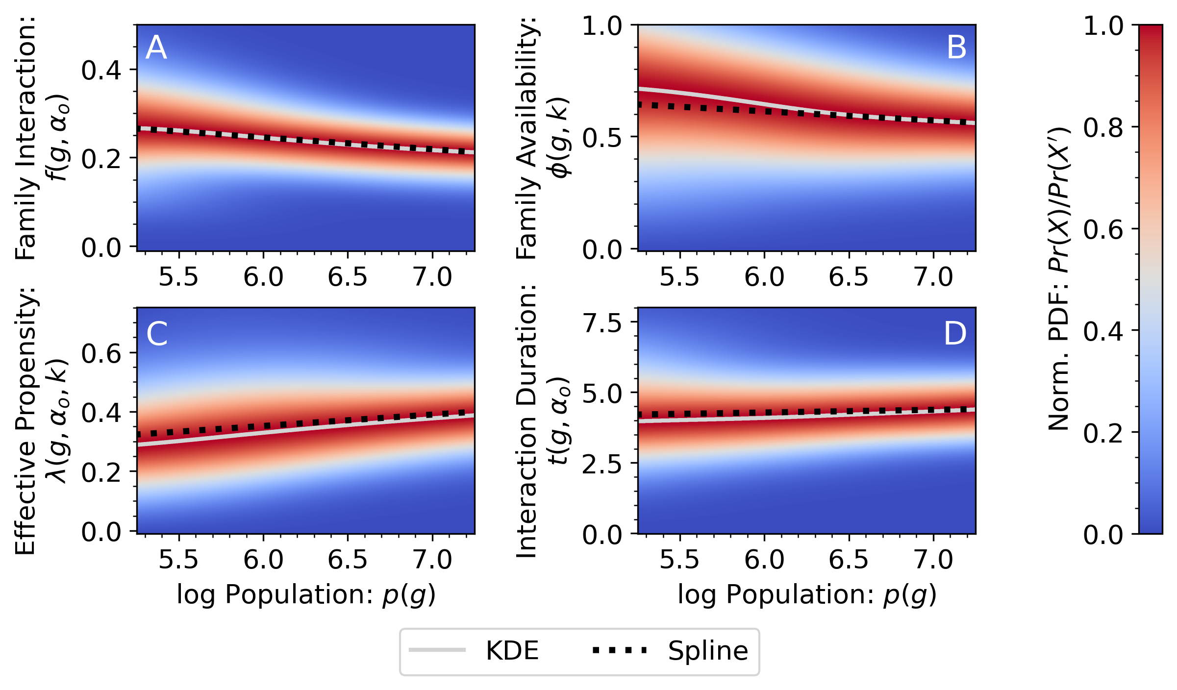
Figure 1: Heat maps of normalized densities, conditional on city population, of interaction $f$ (panel A), availability $\phi$ (B), propensity $\lambda$ (C), and interaction duration $t$ (D). Densities for each of the quantities are calculated using pairs of points, one for each city $g$, where the horizontal coordinate is $p(g)$ and the vertical coordinate is the quantity ($f$, $\phi$, $\lambda$, and $t$) evaluated at $g$. The densities are generated using kernel density estimation (KDE). The normalization of the conditional density is done with respect to the probability of the mode of said density. Red represents large values of the normalized density (approaching $1$) whereas blue represents small values. For the relevant panels, $\alpha=\alpha_{o}$, which represents any activity done on any type of day (weekday or weekend) with nclf. The light gray line in each plot corresponds to the modal regression line of each plot (the line of most probable values of the normalized conditional density). The black dashed line corresponds to the smoothing spline for the same points that generate the heat map. While $f$, $\phi$, and $\lambda$ are normalized quantities ranging from $0$ to $1$, and representing a fraction of people, $t$ is a time, measured in hours. Both interaction (panel A) and availability (B) show decaying trends with population, apparent from the decay of the modal line, the smoothing spline, and the red bands. On the other hand, propensity and duration of interaction both increase with population. All relevant displayed plots are parameterized with $k=3$ in $\phi$, the number of nclf contacts in a city one considers to be needed for nclf interaction to occur. Robustness checks on the effects of survey sample size are provided in Supplementary Section 2.

We first apply non-parametric modal regression to identify the typical behavior of $f$ with respect to $p$. This regression is based on estimating through kernel density estimation (KDE) the conditional probability density $\rho(f\>\lvert\>p,\alpha)$ and its conditional mode $f^{*}(p,\alpha)$, the value of $f$ given $p$ for which $\rho(f\>\lvert\>p,\alpha)$ is largest. We first apply the method to the most general $\alpha=\alpha_{o}=\text{(any activity, any day)}$; this choice of $\alpha$ also provides a useful baseline against which to compare all other results. The light-gray curve in Fig. 1A shows the mode $f^{*}$ as a function of $p$. We can clearly observe the systematically decaying trend of $f^{*}(p,\alpha_{o})$ as a function of $p$. For the smallest log-population $p(g)\approx 4.958$, $f^{*}(g,\alpha_{o})$ is estimated to be $0.267$; for the large limit $p(g)\approx 7.286$, $f^{*}(g,\alpha_{o})\approx 0.211$. This represents an overall drop of $\approx 0.056$, i.e., about $21\%$ of interaction over the log-population range. The concrete form of the trend of $f^{*}$ with $p$ appears to be slightly slower than linear.

Figure 1A also displays a heatmap of the conditional probability density $\rho(f\>\lvert\>p,\alpha_{o})$ scaled by $\rho(f^{*}\>\lvert\>p,\alpha_{o})$. The color represents a normalized scale across values of $p$ of the location of the probability mass (note that $\rho(f\>\lvert\>p,\alpha_{o})/\rho(f^{*}\>\lvert\>p,\alpha_{o})=1$ when $f=f^{*}$). The concentration of $\rho(f\>\lvert\>p,\alpha_{o})$ above and below $f^{*}(p,\alpha_{o})$, expressed by the intense red color, crucially suggests that $f(g,\alpha_{o})$ is typically quite similar to $f^{*}(p(g),\alpha_{o})$, the point on the modal regression corresponding to the population $p=p(g)$ of $g$. In addition, since $f^{*}(p(g),\alpha_{o})$ has a systematically decaying trend with $p$, it means that in general $f$ also decays with $p$.

Aside from the typical behavior of $f$ with $p$, we also analyze its average behavior via the well-known method of cubic smoothing splines wang2011smoothing . In this method, the average behavior is captured by the function $f^{(b)}(p\>\lvert\>\alpha_{o})$ that minimizes the sum of quadratic errors between $f^{(b)}(p\>\lvert\>\alpha_{o})$ and the data plus a cost for curvature in $f^{(b)}(p\>\lvert\>\alpha_{o})$ which controls for over-fitting. The fitted spline is shown as the black dotted curve in Fig. 1A, and exhibits a similar decay pattern as the modal regression.

The decay of $f^{*}$ and $f^{(b)}$ with respect to $p$, observed in Fig. 1 for $\alpha_{o}$ is not an isolated effect. We now expand our analysis to include ‘social’ and ‘care’ activities reported by the ATUS respondents, defined as $\alpha_{\text{social}}=\text{(any social activity, any day)}$ and $\alpha_{\text{care}}=\text{(any care activity, any day)}$, respectively (see Supplementary Table 4 for the ATUS activity types we consider to be social or care-related). Using these new aggregate activity-days ($\alpha_{\text{social}}$ and $\alpha_{\text{care}}$) leads to similarly decaying modal regressions with respect to $p$. These can be seen in Fig. 2A (inset), where we can also notice that, depending on the specific $\alpha$, the range of values of $f^{*}(p,\alpha)$ also changes. For example, $f(g,\alpha_{\text{social}})$ ranges from about $0.226$ to $0.181$ as population increases, a range that is not very different from that of $f(g,\alpha_{o})$, whereas $f(g,\alpha_{\text{care}})$ is constrained to the range from $0.078$ to $0.058$ over the population range.

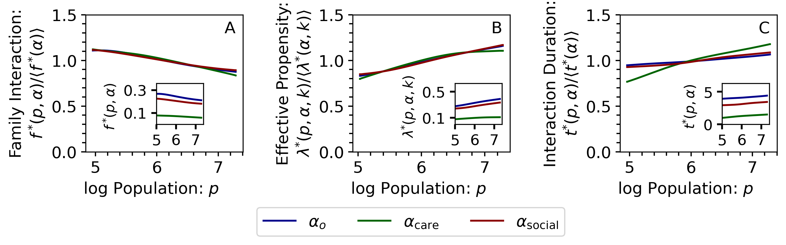
Figure 2: Shown in A) is the scaled KDE modal regression for family interaction, $f^{*}\!(p,\alpha)$, for select $\alpha$, scaled to the expected value $\langle f^{*}\!(\alpha)\rangle$ of each $\alpha$. The inset plot shows the corresponding result without scaling. Similarly, B) illustrates the same for effective propensity, $\lambda\!^{*}\!(p,\alpha,k)$, in the primary and inset plots, and C) shows shows the corresponding results for $t^{*}\!(p,\alpha)$ in hours. Note that $\lambda$ is parameterized with $k=3$. Panels A and B show complete collapses (overlaps) of the lines in their scaled versions indicating that the population trends of both $f^{*}\!(p,\alpha)$ and $\lambda\!^{*}\!(p,\alpha,k)$ are not greatly affected by $\alpha$, suggesting an underlying common trend independent of $\alpha$. In Panel C, $\alpha$ associated with care is the only modal line that fails to collapse, which suggests that the actual duration of care activities may last longer as population increases, which may reflect additional behavioral mechanisms in need of further research.

Following the conceptual framework we proposed in the Introduction, we would want to know whether these decaying trends in $f$ with $p$ originate from availability or propensity. The fact that these trends persist across three different activity-days is suggestive of the hypothesis that availability is the origin of the consistent decay because it is independent of timing and activity by definition. Under this hypothesis, propensity would explain the relative differences in interaction given a specific activity-day based on people’s likelihood of interacting with nclf given the nature of the engagement. If availability exhibits a decaying trend, the combination of $\alpha$-independent availability and $\alpha$-dependent propensity could generate the observed interaction behavior. To test this possibility with $f^{*}$ and the $\alpha$s already in Fig. 2A (inset), we perform a scaling of $f^{*}(p,\alpha)$ by its average, given by $\langle f^{*}(\alpha)\rangle:=\int_{p_{\min}}^{p_{\max}}f^{*}(p,\alpha)dp/(p_{\max}-p_{\min})$. The rescaling leads to the main part of Fig. 2A in which we can see that the curves for the three different $\alpha$ overlap (collapse). The collapse suggests that the decaying trends for each of the $\alpha$s are not unrelated but, instead, are driven by a shared function that is independent of $\alpha$ (if it was $\alpha$-dependent, the functional forms of $f^{*}(p,\alpha)/\langle f^{*}(\alpha)\rangle$ with respect to $p$ would be different and, hence, not collapse). Although this result is not in itself proof that the hypothesis just presented is correct, it does suggest that independent analyses of availability and propensity are warranted. The last method of analysis we employ to study the relation between $f(g,\alpha)$ and $p(g)$ is weighted least squares (WLS). First, we corroborate that the set of aggregate activities (Tab. 1, top section), corresponding to the three cases of $\alpha$ discussed above, display negative significant regression coefficients ($\beta_{1}$). Note that, since $f^{*}(p,\alpha)$ in Figs. 1A and 2A shows a non-linear decaying trend, there is value in going beyond the analysis of averages based on WLS and smoothing splines.

	$\beta_{1}$	Adj. $R^{2}$	0.025	0.975	$\beta_{1}$	$\Sigma_{i}a_{i}(\alpha)$
Aggregate activity	$f(g,\alpha)$				$\lambda(g,\alpha)$
Any	-0.031***	0.116	-0.041	-0.021	0.032**	7694
Social	-0.026***	0.099	-0.036	-0.017	0.027**	6554
Care	-0.015***	0.070	-0.021	-0.008	0.002	2366
Individual activity	$f(g,\alpha)$				$\lambda(g,\alpha)$
Social & Leisure	-0.024***	0.106	-0.032	-0.015	0.017*	5312
Care, Non-Coresid	-0.010***	0.043	-0.016	-0.005	0.004	1849
Eating & Drinking	-0.009**	0.016	-0.017	-0.001	0.026***	3892
Household	-0.009***	0.033	-0.014	-0.003	0.005	1813
Care, Coresid	-0.006***	0.033	-0.009	-0.002	-0.003	623
Traveling	-0.005	0.004	-0.012	0.002	0.026***	2951
Consumer Purchases	-0.005**	0.015	-0.009	-0.000	0.006	1134
Religious	-0.004***	0.026	-0.007	-0.001	-0.004*	394
Sports, Exrc. & Rec.	-0.004**	0.014	-0.007	-0.000	0.001	485
Volunteer	-0.002**	0.016	-0.003	-0.000	-0.001	125
Work	-0.000	-0.004	-0.002	0.002	0.002	238
Personal Care	-0.000	-0.003	-0.001	0.001	0.000	45
Phone Calls	-0.000	-0.004	-0.002	0.001	0.001	102
Govt Serv. & Civic	0.000	-0.000	-0.000	0.001	0.001*	15
Household Svc.	0.000	-0.003	-0.001	0.001	0.001	43
Prof. & Pers. Svc.	0.000	-0.003	-0.001	0.002	0.002	162
Education	0.001	0.005	-0.000	0.002	0.002*	37
Community	$\phi(g,k=3)$
Family Availability	-0.048**	0.023	-0.086	-0.010	–	1706

Table 1: Weighted Least Squares analysis of the dependence of interaction $f$, availability $\phi$, and propensity $\lambda$ of cities as functions of their log-population sizes. Aggregate $\alpha$s are shown at the top, followed by specific ATUS $\alpha$, and finally, $\phi$ calculated with $k=3$ from the PSTS. For this table, all $\alpha$ distinguish activities but combine type of day of the week (weekday and weekend). Most slope coefficients associated with $f$, and all the significant ones, are negative. In contrast, the majority of coefficients for $\lambda$ are positive, with only one significant coefficient with a small negative slope (corresponding to interaction with nclf for religious activity, a trend that may reflect cultural trends). Significance levels correspond to *$p<.10$, **$p<.05$, and ***$p<.01$.

Given the consistency uncovered for the aggregate activities, it is pertinent to explore whether decaying trends also hold for other ATUS major category activities. There are three reasons for this: (i) aggregations of several activities could be susceptible to Simpson’s paradox, generating spurious trends by way of aggregation, (ii) if indeed a decaying trend in availability is affecting $f(p,\alpha)$ systematically over $\alpha$, further evidence would be garnered by doing this analysis, and (iii) for different reasons, both modal regression and smoothing spline results are not as reliable for $\alpha$s that do not occur often (see last column of Tab. 1). The $\beta_{1}$ column of Tab. 1 under the area of “Individual activity” shows these results, which further support our thinking. Indeed, the regression coefficients for many individual activities are negative and statistically significant. The preponderance of significant negative slopes indicates that the trends observed using aggregate $\alpha$s (such as for Figs. 1 and 2A) are not affected by aggregation effects, strengthening the case for an $\alpha$-independent availability that decays with $p$. Before proceeding to test availability, we note that the decaying trend in nclf interaction with population is not due to an overall decay of interaction with all non-household contacts (family or not) in big cities. On the contrary, data shows that interaction with non-household contacts in fact increase as cities get larger (see Supplementary Section 3).

2.2 Availability

Although the ATUS does not provide data to directly test any trend of nclf availability with $p$, this can be done by leveraging a survey from the Pew Research Center called the Pew Social Trends Survey (PSTS) PEWsocialtrends . As part of the PSTS, respondents are asked how many family members live within an hour’s drive of where they live, providing a way to measure nclf availability. The PSTS reports this number for each respondent in discrete categories ($0$, 1 to 5, 6 to 10, 11 to 15, 16 to 20, and 21 or more).

In establishing a link between interaction and availability, a pertinent concept that should not be overlooked is that individuals do not engage with their family members on equal footing, nor do they interact with all of them DunbarSpoor ; MOK2007 —an important finding from the literature on ego networks concerned with how much interaction people have with their kin and other kinds of contacts. Instead, individuals place some kinship ties at a high level of importance while relegating others to be of low relevance. To illustrate, while a distant relative may be proximal to somebody in a location, this proximity may play no role because the relative is not particularly important in the person’s social network. In contrast, interacting with, say, a parent, an offspring, a sibling, or the progeny of these family members, is likely to be much more important. This sorting, regardless of which relationships end up being important and which do not, leads to the effect that not every single kinship-tie is necessarily useful to count.

Guided by this theory, we define for each PSTS respondent $i$ a variable $b_{i}(k)$ that takes on the value $1$ when they report having $k$ or more nclf available, and $0$ if they report having less than $k$ nclf. Then, we define a measurement of overall availability for each location $g$ given by

$$\phi(g,k)=\frac{\sum_{i\in g}w_{i}b_{i}(k)}{\sum_{i\in g}w_{i}}.$$ (2)

Similar to the ATUS, each PSTS respondent is given a weight $w_{i}$ that balances the demographic distribution of the sample such that the sample is representative at the national level. Given the categorical reporting of the PSTS variable, we develop an algorithm that allows us to reliably change $k$ by increments of one unit (see Supplementary Section 4.2).

In order to determine the population trend, if any, of $\phi(g,k)$ as a function of $p(g)$, we carry out the modal regression and smoothing-spline analysis again. The results are shown in Fig. 1B. As conjectured, the trends of availability captured by $\phi^{*}(p,k)$ and $\phi^{(b)}(p,k)$, respectively the modal regression and the spline of $\{p(g),\phi(g,k)\}_{g}$, are decaying with respect to $p$. As an additional consistency check for this decay, we calculate the WLS slope coefficient of $\phi(g,k)$ as a function of $p(g)$ and find that it is both negative and significant (see $\beta_{1}$ in Tab. 1, community section). The results presented here, and for the rest of the paper, are for $k=3$. However, varying $k$ does not change the results qualitatively (see Supplementary Figure 6).

The results here support our hypothesis that nclf interaction rates in larger cities are lower than smaller cities because overall nclf availability is also lower in the larger cities, but they do not yet paint a complete picture. One pending and interesting question is how people choose to interact with family that is local to them (their propensity). One should contemplate the possibility that this propensity may also display negative $p$-dependence (i.e., that people in larger cities have lower need or desire to see their family). The results of Sec. 2.1, and perhaps our experience, would suggest that such a behavior may be negligible or even unlikely. Furthermore, consideration of the various functions that nclf perform runs counter to a propensity that decays with $p$. Whilst this simple picture is convincing and in agreement with intuition, none of our analysis so far can determine this. To be able to test propensity, we next introduce a probabilistic framework that can help us discern between behavioral and non-behavioral effects.

2.3 Probabilistic framework for interaction, propensity, and availability

To understand the interplay between availability and propensity that leads to actual interaction, we introduce a probabilistic model where each of these effects is explicitly separated. The model is structured such that it is easy to relate to typical survey data such as what we use here. An in-depth explanation of the model can be found in Supplementary Section 5.

Consider a model with various cities. In a city $g$, any given individual $i$ is assigned two random variables, one that indicates if the individual has nclf available ($b_{i}=1$) or not ($b_{i}=0$), and another that indicates if they report performing $\alpha$ with nclf ($a_{i}(\alpha)=1$) or not ($a_{i}(\alpha)=0$). In addition, individuals in a location $g$ are grouped into population strata within which they all share the same personal characteristics. For example, $i$ may be male, of a certain age range, and a given ethnicity. These characteristics are captured in the vector $\mathbf{c}(i)$. All individuals that share the same vector $\mathbf{c}$ of characteristics represent a segment of the target population, and this induces a set of weights $w(\mathbf{c})$ for each of those individuals such that the sum $\sum_{i\mathchar 24635\relax\;\mathbf{c}(i)=\mathbf{c}}w(g,\mathbf{c}(i))$ is the size of the target population $Q(g,\mathbf{c})$ in $g$ with features equal to $\mathbf{c}$.

For simplicity, we first work with given values of $g$, $\mathbf{c}$, and $\alpha$. We introduce the probability $\kappa(g,\mathbf{c},\alpha)$ that an individual in stratum $\mathbf{c}$ of location $g$ reports doing $\alpha$ with nclf available to them. We think of this as the pure propensity to interact. On the other hand, the probability of available nclf is given by $\phi(g,\mathbf{c})$, which does not depend on $\alpha$. While dealing with given $g$, $\mathbf{c}$, and $\alpha$, we simply use $\kappa$ and $\phi$ and then reintroduce $\mathbf{c}$, $g$, and $\alpha$ when needed. On the basis of these definitions, the joint probability that a given individual has concrete values $a_{i},b_{i}$ is given by

$${\rm Pr}(a_{i},b_{i})=\kappa^{a_{i}}(1-\kappa)^{1-a_{i}}\phi\delta_{b_{i},1}+\delta_{a_{i},0}(1-\phi)\delta_{b_{i},0},\quad[a_{i},b_{i}=0,1],$$ (3)

where $\delta_{u,v}$ is the Kronecker delta, equal to $1$ when $u=v$, and $0$ otherwise. This expression captures all possible combinations of availability and interaction: people without availability have probability $1$ to respond $a_{i}=0$, whereas those with availability, which occurs with probability $\phi$, have a chance of $\kappa\phi$ to report interacting with family and $1-\kappa\phi$ to report not interacting with family.

On the basis of the personal probability captured in Eq. 3, and using $s=s(g,\mathbf{c})$ to represent the number of individuals surveyed in $g$ with $\mathbf{c}$, we can determine the marginal distribution that $y=y(g,\mathbf{c},\alpha)$ individuals report doing $\alpha$ with nclf, equivalent to the probability that there are exactly $y$ individuals in total for whom $a(\alpha)=1$. This marginal is given by the binomial distribution

$${\rm Pr}(y)=\binom{s}{y}(\kappa\phi)^{y}(1-\kappa\phi)^{s-y}.$$ (4)

It is worth remembering that this applies to a specific subset of people in $g$, i.e. those respondents with personal features $\mathbf{c}$.

We now use Eq. 4 and the fact that its expectation is given by $y(g,\mathbf{c},\alpha)=s(g,\mathbf{c})\kappa(g,\mathbf{c},\alpha)\phi(g,\mathbf{c})$ to estimate the model expectation for actual interaction, $f_{m}(g,\alpha)$, which can in turn be related to our data. This calculation is straightforward because the statistics for each $\mathbf{c}$ are independent. Specifically, since each individual with $\mathbf{c}$ in $g$ represents $w(g,\mathbf{c})$ others, $f_{m}(g,\alpha)$ is equal to the weighted average of the expectations $y(g,\mathbf{c},\alpha)$, or

$$f_{m}(g,\alpha)=\frac{\sum_{\mathbf{c}}w(g,\mathbf{c})s(g,\mathbf{c})\kappa(g,\mathbf{c},\alpha)\phi(g,\mathbf{c})}{\sum_{\mathbf{c}}w(g,\mathbf{c})s(g,\mathbf{c})}=\frac{\sum_{\mathbf{c}}Q(g,\mathbf{c})\kappa(g,\mathbf{c},\alpha)\phi(g,\mathbf{c})}{Q(g)},$$ (5)

where the relation between sample weights, size, and population $Q(g,\mathbf{c})=w(g,\mathbf{c})s(g,\mathbf{c})$ has been used, together with the fact that $Q(g)=\sum_{\mathbf{c}}Q(g,\mathbf{c})$. Equation 1 can be interpreted as a trial of the current model, with expectation given by Eq. 5.

2.4 Effective propensity

Ideally, we would like to determine the propensity $\kappa(g,\mathbf{c},\alpha)$ for all $g$, $\mathbf{c}$, and $\alpha$. If data allowed it, we could achieve this by equating the expectation of $y$, given by $s(g,\mathbf{c})\kappa(g,\mathbf{c},\alpha)\phi(g,\mathbf{c})$, with its sample value $\sum_{i\in g}a_{i}(\alpha)\delta_{\mathbf{c},\mathbf{c}(i)}$ (the number of respondents that report doing $\alpha$ with nclf) and solving for $\kappa(g,\mathbf{c},\alpha)$. However, this strategy is hampered by the fact that we do not have enough information to determine $\phi(g,\mathbf{c})$ with sufficient accuracy.

To address this limitation, we employ a different strategy that is able to provide valuable information about propensity at location $g$ for each $\alpha$. To explain it, we begin by noting that availability can be written on the basis of $\phi(g,\mathbf{c})$ as

$$\phi(g)=\frac{\sum_{\mathbf{c}}Q(g,\mathbf{c})\phi(g,\mathbf{c})}{Q(g)}.$$ (6)

Next, we introduce the quotient between interaction and availability calculated from the model. We call this quotient $\lambda(g,\alpha)$, the effective propensity of interaction. It is given by

$$\lambda(g,\alpha)=\frac{f_{m}(g,\alpha)}{\phi(g)}=\frac{\sum_{\mathbf{c}}\kappa(g,\mathbf{c},\alpha)Q(g,\mathbf{c})\phi(g,\mathbf{c})}{\sum_{\mathbf{c}}Q(g,\mathbf{c})\phi(g,\mathbf{c})}.$$ (7)

In this expression, $\lambda(g,\alpha)$ is a weighted average of $\kappa(g,\mathbf{c},\alpha)$ over the part of the population of $g$ that does have nclf available (where the weights are $Q(g,\mathbf{c})\phi(g,\mathbf{c})$). In other words, it constitutes the effective average of propensity.

Whilst Eq. 7 allows us to interpret the meaning of $\lambda(g,\alpha)$, its calculation is straightforwardly done by using the sample values $f(g,\alpha)$ and $\phi(g)$ given respectively by Eqs. 1 and 2. Fig. 1C, we show the modal regression $\lambda^{*}(g,\alpha_{o})$ and smoothing-spline $\lambda^{(b)}(g,\alpha_{o})$ for the set of points $\{(p(g),\lambda(g,\alpha_{o}))\}_{g}$. Both curves show that population size has a very small increasing effect on $\lambda(g,\alpha_{o})$, from which we can deduce that the propensity to interact with nclf for those people that have nclf available is not being limited or reduced by $p$.

As with $f^{*}(p,\alpha)$, $\lambda^{*}(p,\alpha)$ for the aggregate $\alpha_{o}$, $\alpha_{\text{social}}$, and $\alpha_{\text{care}}$ also collapse when divided by their averages $\langle\lambda^{*}(\alpha)\rangle:=\int_{p_{\min}}^{p_{\max}}\lambda^{*}(p,\alpha)dp/(p_{\max}-p_{\min})$ (Fig. 2B). Although this may superficially appear unsurprising given the relations between $f$, $\phi$, and $\lambda$ (Eq. 7), it is worth keeping in mind that $\lambda^{*}(p,\alpha)$ is the directly estimated conditional mode of the $\lambda(g,\alpha)$ data. Thus, the collapse suggests that the trends that govern the values of $\lambda(g,\alpha)$ for individual cities are indeed multiplicative: a product of a $\phi$ dependent on $g$ but independent of $\alpha$, and a pure propensity $\kappa$ dependent on $\alpha$, predominantly.

A more comprehensive analysis of trends of $\lambda$ with respect to $p$ is performed through WLS, shown in Tab. 1 (fifth column) for the remaining $\alpha$s in the ATUS. There are $8$ significant coefficients, of which only religious activities has a negative slope, albeit with a very small value; the remaining significant coefficients are positive. Among all coefficients (significant and non-significant), only $3$ coefficients altogether have negative slopes. This shows the predominant tendency for the effective propensity to either increase slightly with $p$ or be roughly independent of it.

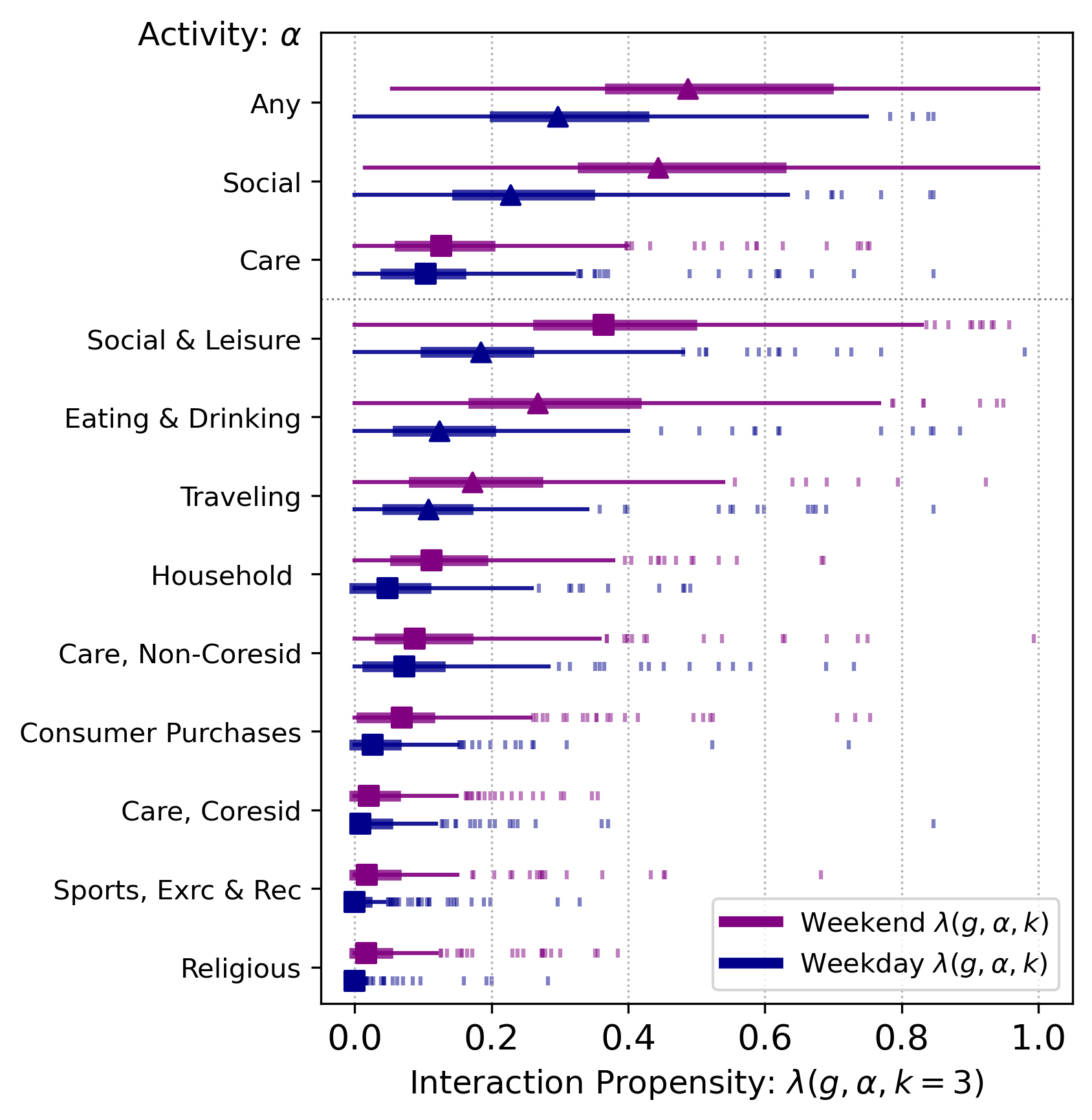
Figure 3: Box plots of interaction propensities $\lambda(g,\alpha,k)$ for well-sampled $\alpha$s in ATUS, along with aggregate $\alpha$ (at the top). Here, weekends and weekdays have been kept separate to distinguish the changes in propensity with respect to this variable. The triangles and squares are located at the point of median of the $\lambda(g,\alpha,k)$ for a given $\alpha$. Triangles pointing up represent an increasing trend of the propensities with $p$ and squares represent no significant increasing or decreasing trend, consistent with the results on Tab. 1; triangles pointing down would appear if a significant decaying trend was present, but none are obtained. The bold lines represent the IQR, thin lines the minimum of the remaining range observed or $1.5\times$IQR in each direction, and the remaining points (the outliers) are denoted with pipe-marks. The selected activities were filtered to remove those with medians not noticeably above 0. These box plots show which activities respondents choose to do with family, ordered by aggregation followed by propensity.

Having studied the propensity $\lambda$ with respect to $p$, we now focus on how various activity-days $\alpha$ affect it. In Fig. 3, we present box plots of the sets of values $\{\lambda(g,\alpha)\}_{g}$ for those activity-days that are sufficiently well-sampled. Here, we make a distinction between weekday and weekend when constructing $\alpha$s. Median values are represented by the triangle and square shapes. Triangles point up if $\lambda$ of a given $\alpha$ shows a statistically significant increase with $p$ and squares indicate that $\lambda$ has no significant trend with $p$. No statistically significant decreasing trends of $\lambda$ with $p$ were observed for any $\alpha$. The trends and their significance correspond to those in Tab. 1. Aggregate versions of $\alpha$ are placed at the top of the figure to provide a reference. As expected, people exhibit a larger propensity to interact with nclf on weekends than on weekdays for all activity categories. Spending social time with family has the largest propensity with weekend median value of $0.44$, which can be interpreted as the chances that an individual with nclf available would do a social activity with them on a weekend are approximately $44\%$, in marked contrast to weekdays when the propensity drops to $22.7\%$. In comparison, care-related activities have weekday propensities of $10.4\%$, increasing slightly to $12.6\%$ on the weekends. Another observation from Fig. 3 is that the ranges of values of $\lambda$ can be large for the most common activities. The values of $\lambda$ can be used for estimation of interaction in a variety of cases. For example, assuming independent random draws with $\lambda$ as the success rate for any given $\alpha$, we can quickly estimate such quantities as the proportion of people (in a city or nationally) that meet with nclf in a period of time (say, a month) to do $\alpha$, or the average wait time until the first meeting to do $\alpha$.

To complete our analysis of $\lambda$, we present two other summary results in Supplementary Section 7. First, we provide a rank-ordered reference of activities by propensity averaged over the US in Supplementary Table 4. This shows which activities are associated with high or low propensity. Second, to learn about how values of $\lambda(g,\alpha)$ are distributed across concrete US metropolitan areas, and particularly which places exhibit either considerably larger or smaller propensities than other cities of similar populations, we also present Supplementary Table 5, which shows the top and bottom $10$ locations by average rank-order based on weighted $z$-scores of $\lambda(g,\alpha)$ with respect to $\lambda^{*}(p(g),\alpha)$, where ranks are averaged for values of k ranging from 1 to 3. Similar analysis is conducted for interaction duration $t$ (defined next) and shown in Supplementary Table 6.

2.5 Interaction duration with nclf family

As a final analysis of the interplay between people’s nclf interaction and population size, we study one last quantity captured in ATUS: the interaction duration with nclf. The relationship between interaction duration and population size can also be studied with the techniques we have used thus far.

Let us denote the duration of $i$’s interaction with nclf for $\alpha$ by $t_{i}(\alpha)$. Thus, for a given location $g$ and $\alpha$, the average interaction duration is given by

$$t(g,\alpha)=\frac{\sum_{i\in g}w_{i}t_{i}(\alpha)a_{i}(\alpha)}{\sum_{i\in g}w_{i}a_{i}(\alpha)},$$ (8)

where $a_{i}(\alpha)$ is defined the same way as in Eq. 1. Note that interaction duration is averaged only over those that report nclf interaction for the $\alpha$ under consideration. This is because $t$ clearly involves a behavioral component, and we are interested in determining the role that population size may exert in the behavior of people when they interact with nclf. If an increase in $p$ was associated with a decrease in the duration of interaction, it could suggest, for example, that people’s busy lives in larger cities limit how much they are able to interact with family, which could be a signal associated with the decaying trends for $f$.

In Figs. 1D and 2C we present examples of modal regressions and smoothing splines of interaction duration $t$ with respect to $p$ for aggregate $\alpha_{o}$, $\alpha_{\text{social}}$, and $\alpha_{\text{care}}$. In all cases, $t^{*}(g,\alpha)$ and $t^{(b)}(g,\alpha)$ are either approximately steady over $p$ or increasing slightly. As in the case of propensity, interaction duration captures the behavioral dimension of interaction. The lack of a decaying trend provides further support for the notion that family availability may be the main driver of interaction decay and that people’s attitudes towards interacting with family are not diminished by population size.

3 Discussion

The separation of interaction into two necessary factors, availability and propensity, provides a new lens by which to understand it in a more coherent and principled way. Over relatively short periods of time (say, weeks or months) and at the population level of cities, patterns of availability are rigid, which is to say they are structural and approximately fixed in time and space. On the other hand, patterns of propensity are due to day-to-day decision-making and encompass the bulk of the agency that individuals have in controlling interaction at any given time in the short term; propensity is much more flexible than availability, and generally operates at shorter time scales. If we phrased interaction in the language of social networks, availability can be thought of as a static well-defined social network based purely on underlying formal social relations (unambiguously defined for nclf, e.g., parent, sibling, in-law), while propensity is a stochastic process occurring on the static network.

Perhaps the most salient observation we make is that, at the level of population of cities, availability explains the heterogeneity in nclf interaction, effectively providing clear support for our approach. In addition, for most activities propensity shows either a weak positive population-dependent trend or no trend. This supports another one of our most important conclusions that, when family is locally available, people take ample advantage of their presence to interact with them. Moreover, the time invested in those interactions are not negatively impacted by population size (i.e., the busy lives of residents of big cities do not deter them from spending time with family). Phrased in social network theory terms, our results imply that the static social networks of nclf differ by city and those differences are the main drivers of the differences in face-to-face interaction we observe, and that nclf propensity is roughly independent of the structure of these networks.

This robust family-interaction effect may have important consequences in how people shape the rest of their social networks DAVIDBARRETT201720 ; personal-networks . At a more fundamental level, if availability plays a dominant role in nclf interaction, the patterns that characterize this availability are also likely to characterize other critical aspects of life that strongly depend on nclf interaction (say, care-related outcomes COMPTON2014 ; taylor1986patterns ; MCCULLOCH1995 or certain aspects of people’s well-being DunbarSpoor ; MOK2007 ; roberts2015managing ).

As suggested in the Introduction, another aspect that depends on interaction is propagation of infectious diseases. Current research in epidemiological modeling does not pay attention to the concepts of availability and propensity when dealing with interaction data. Consider, for example, the large scale European POLYMOD survey concerned with determining population mixing matrices capturing patterns of social contacts Mossong , frequently used in population-level epidemiological modeling in Europe. Availability is not tracked in this survey (or most other population-level surveys of interaction), but such information can prove critical when large disruptions to regular patterns of behavior (i.e. propensity) can take place, such as has been observed during the COVID-19 pandemic. For one, availability in most cases would not change in the rapid way propensity can change. Also, the way that propensity can adjust after the start of a pandemic is constrained by availability; i.e., availability is a template inside of which propensity can adapt to pandemic conditions. While not all study of human interaction is aimed at such extremes, the framework of availability and propensity still applies. Furthermore, because the fundamental concepts of availability and propensity are not restricted merely to family ties, our remarks here are relevant to social interactions generally.

All the examples provided above can lead to policy considerations. Many non-pharmaceutical interventions applied during the COVID-19 pandemic have been directed at reducing propensity for face-to-face interaction or aiding those with economic needs (see PERRA20211 for a review of intervention), but they have hardly considered availability, which may reflect structural needs of the populations of those places. In low-income areas, family support to take care of young children COMPTON2014 is an economic necessity. Asking people in such locations to stop seeing family may prove ineffective. In places with low nclf availability, the closure of daycare during the COVID-19 pandemic coupled with the lack of family support could lead to more mothers dropping out of the workforce, perpetuating gender inequality and slowing down economic recovery. Thus, policy interventions that consider these needs at the local level would likely have a better chance at being effective Hale2021 . From the standpoint of other support roles performed by nclf, a better measurement and understanding of the interplay between availability and interaction may inform how to best address the needs of people at a local level in ways not unlike those that address housing, education, or other locally-oriented policy making.

The origin of the population pattern displayed by availability, although not our focus here, is likely related to domestic migration litwak1960occupational ; litwak1960geographic . The more pronounced absence of family in larger populations may be driven by the fact that larger cities tend to offer a variety of opportunities for work, education, and access to particular services and amenities not always available in cities with smaller populations, thus generating an in-migration that is, by definition, a source of decreased family availability. In this scenario, one of the main drivers of the population trend in availability would be economic (see similar examples KANCS2011191 ), suggesting a feedback mechanism whereby the in-migration leading to less family availability can be improving or sustaining economic success, in turn perpetuating the incentives for that in-migration over time. However, other mechanisms such as a desire to maintain close ties with family are likely to balance the economic incentives, preventing the feedback from becoming a runaway effect LEWICKA ; Spring ; litwak1960geographic ; litwak1960occupational . Note that this last point does suggest a coupling between availability and propensity that operates at long time scales (say, over one or multiple years), by which the fraction of the population that is not willing to be far from extended family would exercise agency to adjust their living conditions through migration to be closer to family.

Our study contains certain limitations. First, while demographic characteristics are incorporated into our model, estimates of propensity and availability for specific demographic strata are not obtained here due to limitations in survey sampling. Such demographic understanding of interaction is important and should be considered in future research if appropriate data can be obtained. Second, although the ATUS tracks a substantial variety of activities, one should not view it as a comprehensive catalog of all possible ways in which people may interact. To name one example, activities that involve more than a single day are not currently collected in the ATUS by design. Other such limitations exist and researchers should be mindful of that. Third, it may prove fruitful to consider material availability that could affect interaction (for example, in a city without a cinema an $\alpha$ for going to the movies would have propensity $=0$). We do not expect this factor to play a major role for the $\alpha$s and locations we study, as our smallest cities have populations of $\approx 130,000$ people. However, investigations focused on more detailed activities in smaller places could require taking this effect into account. Fortunately, the structure of our model can be straightforwardly updated to include such material availability given sufficient data.

At a methodological level, there are interesting observations our work suggests. For example, some simple modifications to large-scale surveys of people’s interaction and time-use behavior could lead to extremely beneficial information able to enhance the usefulness of such surveys. The ATUS could add a few simple questions to their questionnaires that would determine whether respondents have family, friends, or other contacts locally available to them even if no activities have been performed with them. Such questions could provide baseline information about not just what people do but their preferential choices, helping to distinguish the effects of both propensity and availability on interaction.

As a final reflection, we relate the notions of availability and propensity to the very successful discipline of network science and its application to spreading processes on social networks newman2018networks ; VespignaniReview ; Havlin ; HOLME201297 ; porter2016dynamical . In this theoretical context, our concept of availability translates to a static network structure of social connections that exist independent of contact activity. Propensity, on the other hand, would be represented by a temporal process of contact activity occurring on the static network. In this context, what the results of the present work mean for the study of processes on networks is that realistic models need to take into account the heterogeneity in both the types of ties (network links) and their associated contact processes. In the case of epidemics, the introduction of frameworks such as those in Karrer ; Karsai offers great promise because they are compatible with the non-trivial structure we uncover here. This contrasts with most other literature that basically conceives of what we call propensity as a low-probability, permanent contact process occurring with all contacts of the static network (the Markovian assumption VespignaniReview ), a modeling choice that destroys most of the true complexity of the process. Dedicated data that addresses propensity will go a long way in driving the development of a new generation of more realistic models of propagation processes on networks.

In summary, we decompose face-to-face interaction with non-coresident local family at the city level in terms of availability and propensity to interact, and find that while availability decays with the population of those cities, neither the propensity to interact across activities nor the duration of those interactions shows the same decay. The decay in availability is sufficient to lead to an overall decay of interaction with nclf across US cities as their population increases. We arrive at these results by introducing a stochastic model that allows us to combine existing survey data, the American Time Use Survey and Pew Research Center’s Social Trends Survey, to estimate availability and propensity at the US metro level. Analysis of the resulting propensities show that social activities are the most common, especially on weekends. In social networks terms, availability can be thought of as static social networks of family relations and propensity as a process on these networks. Our findings indicate that the availability network differs by city and is the main driver of the variance in observed face-to-face interaction, while propensity is roughly independent of the network structure. We also discuss some of the implications of our framework and offer ideas on how it is relevant for survey-design, scientific research, and policy considerations with some particular attention to the context of the COVID-19 pandemic.

4 Material and methods

4.1 Weighted least squares

Since location sample sizes diminish with population, much of our analysis utilizes weightings. One method we employ is weighted least squares (WLS), defined on the basis of the model

$$v_{g}=\beta_{1}u_{g}+\beta_{o}+\epsilon_{g},$$ (9)

where $g$ indexes the data points, and the error terms $\epsilon_{g}$ do not necessarily have equal variance across $g$ (heteroskedastic). The solution to the model is given by the values of the coefficients $\beta_{1}$ and $\beta_{o}$ such that $\sum_{g}w_{g}\epsilon_{g}^{2}$ over the data points is minimized. The $w_{g}$ correspond to $g$-specific weighing used to adjust how much the regression balances the importance of the data points.

The Gauss-Markov Theorem guarantees that the weighted mean error $\sum_{g}w_{g}\epsilon_{g}^{2}$ is minimized if $w_{g}=1/\text{var}(\epsilon_{g})$. On the other hand, it is known that the variance in a survey is inversely proportional to the size of the sample. Therefore, in our analysis we use

$$w_{g}=\frac{1}{\text{var}(v_{g})}=\frac{s(g)}{\sum_{g}s(g)}\quad(\text{for }v_{g}=f(g,\alpha),\phi(g),\lambda(g,\alpha),t(g,\alpha)),$$ (10)

where $s(g)$ is the number of respondents in $g$. These weights apply to $f(g,\alpha)$ from the ATUS as well as $\phi(g)$ from the PSTS, where the same $g$ may have different relative weights based on the samples collected for each survey in the same location $g$.

To compute these weights when the dependent variable is $\lambda(g,\alpha)$, we make use of the technique called propagation of error. For $\lambda(g,\alpha)=f(g,\alpha)/\phi(g)$, its variance is given as a function of the variances of $f(g,\alpha)$ and $\phi(g)$, calculated through a Taylor expansion up to order $1$. In the limit of weak or no correlation between $f(g,\alpha)$ and $\phi(g)$ (which is reasonable here given that the variables are independently collected),

$$\text{var}(\lambda(g,\alpha))\approx\left(\frac{\partial\lambda}{\partial f}\right)^{2}\text{var}(f(g,\alpha))+\left(\frac{\partial\lambda}{\partial\phi}\right)^{2}\text{var}(\phi(g)).$$ (11)

Assuming the covariance between $f(g,\alpha)$ and $phi(g)$ is negligible, we calculate

$$w_{g}\approx\left[\left(\frac{\partial\lambda}{\partial f}\right)^{2}\text{var}(f(g,\alpha))+\left(\frac{\partial\lambda}{\partial\phi}\right)^{2}\text{var}(\phi(g))\right]^{-1}\quad(\text{for }\lambda(g,\alpha)),$$ (12)

where both $\text{var}(f(g,\alpha))$ and $\text{var}(\phi(g))$ are given by the Eq. 10.

4.2 Weighted cubic smoothing splines

One of the techniques we employ to approximate the functional dependence between $p$ and, separately, $f$, $\phi$, $\lambda$, and $t$ is cubic smoothing splines wang2011smoothing , defined as follows. For two generic variables $u_{g}$ and $v_{g}$, the cubic smoothing spline $v^{(b)}(u_{g})$ is a piecewise smooth function that minimizes

$$\sum_{g}w_{g}(v_{g}-v^{(b)}(u_{g}))^{2}+\eta\int_{\min_{g}\{u_{g}\}}^{\max_{g}\{u_{g}\}}\left(\frac{d^{2}v^{(b)}}{d\xi^{2}}\right)^{2}d\xi,$$ (13)

where $\eta$ is a penalty parameter that controls how much to discourages $v^{(b)}$ from large amounts of curvature (and thus overfitting), and $\xi$ is a dummy variable. In the limit of $\eta=0$, curvature is not penalized and the algorithm overfits the data; when $\eta\to\infty$, the only possible solution requires $d^{2}v^{(b)}/d\xi^{2}\to 0$, leading to a straight line and thus making the algorithm equivalent to weighted least squares (WLS). In the algorithm we employ WOLTRING1986104 , the function $v^{(b)}$ is constructed from cubic polynomials between the data points along $\{u_{g}\}_{g}$, with the condition that they are smooth up to the second derivative along consecutive pieces.

The penalty parameter $\eta$ can be either chosen arbitrarily or, instead, determined on the basis of some selection criterion. In our case, we use generalized cross-validation Golub , which optimizes prediction performance. The algorithm is implemented as the function make_smoothing_spline of the package scipy.interpolate in python splines .

4.3 Modal regression using kernel density estimation

Another method we employ to estimate how population $p$ affects $f$, $\phi$, $\lambda$, and $t$ is non-parametric modal regression. ChenMode . Intuitively, the method looks for the typical behavior of a random variable as a function of some independent variable.

This method is defined in the following way. Using a smoothing kernel (in our case Gaussian), we construct the $2$-dimensional kernel density estimator $\rho(u,v)$ for the set of data points $\{(u_{g},v_{g})\}_{g}$ hastie2009elements , where we choose bandwidth by inspection in the neighborhood of the Silverman method silverman1986density but favor solutions that tend towards the smoothing spline results as they are a sign of a stable modal regression line (details can be found in Supplementary Section 6). Then, we determine the conditional density $\rho(v\>\lvert\>u)=\rho(u,v)/\rho(u)$ and extract its local mode $v=v^{*}(u)$. Here, we use this method for unimodal $\rho(v\>\lvert\>u)$ (multimodality can be handled by the method, but is not relevant here).

4.4 Data

Our interaction data is derived from the American Time Use Survey (ATUS) conducted by the Bureau of Labor Statistics (BLS) ATUS . Each year, the ATUS interviews a US nationally-representative sample regarding their full sequence of activities through the day prior to the interview, termed a diary day. The information collected in this process is recorded in several files, including the “Respondent”, “Activity”, and “Who” data files. We link these files for the period between 2016-2019 to get comprehensive information about each respondent, activities they carried out on the diary day, as well as those who accompanied the respondent during each activity. We consider nclf to be companions of the respondent who are family but do not reside in the same household (see Supplementary Table 2). These may include the respondent’s parents, parents-in-law, own children under 18 years of age, and other family members as long as they do not reside with the respondent. Activities are encoded in the ATUS with codes of $6$ digits, the first two representing activity categories such as ’eating & drinking’, ’personal care’, or ’work’, to name a few. Additional digits provide more specificity about the activity such as the context or some other detail. We restrict our analysis to activities at the two-digit level (called major categories in the ATUS lexicon) which encompass seventeen such codes. The ATUS also captures the day of the week when the respondent has been interviewed, which in known to play an important role in the choices of activities people perform. We encode the combination of activity and type of day with the 2-dimensional vector variable $\alpha$. Therefore, as an example, eating and drinking with family done on a weekend day corresponds to a specific value of $\alpha$. Beyond the use of the ATUS 2-digit codes, we also create aggregate activity categories that serve as baselines to our analysis and capture people’s major social functions. At the most aggregate level, we define $\alpha_{o}$ which combines all activities in the ATUS done on either type of day (weekday or weekend), which we refer to as ’any activity, any day’. We also define $\alpha_{\text{social}}$, the aggregate set of social activities with the 2-digit codes $11-14$ done any day of the week. Finally, we define $\alpha_{\text{care}}$, we combine the 2-digit codes $3-4$ on any day of the week.

To estimate local family availability, we use the Pew Social Trends Survey (PSTS) from the Pew Research Center which was conducted in 2008 using a nationally-representative sample of 2,260 adults living in the continental US PEWsocialtrends . The PSTS identifies geographic location of the respondents at the county level and the binned quantity of family members who live within a one-hour driving distance. To work with the data at the CBSA level, we map county FIPS codes to CBSA codes using the crosswalk downloadable from the National Bureau of Economic Research nbercrosswalk . After filtering by the set of CBSAs common to both surveys, our final sample size is $N=$ 30,061 for the ATUS and $N=$ 1,706 for the PSTS.

Metro populations are obtained from the American Community Survey (ACS) data (5-year estimates, 2015-2019) published by the US Census Bureau censusacs . We also extract various demographic variables from the US Census population estimates to use in the recalibrations of sampling weights (see Weight re-calibration).

4.5 Weight re-calibration

Our analysis of the time variables of the ATUS is performed with consideration to sampling weights. The ATUS provides a sampling weight for each respondent which, in essence, gives an estimated measure of how many people within the US population the respondent represents given the respondent’s demographic and other characteristics. (The unit of these weights is technically persons-day, although for the purpose of our study we normalize by the number of days in the survey period since it simplifies interpretation of the weights to just population, and because our sampling period is fixed.) The use of such weights is meant to reduce bias and improve population-level estimates of quantities captured by the raw survey data. The ATUS respondent weights are calibrated by BLS at the national level which can be reasonable for large cities but are not reliable for smaller CBSAs. For this reason, we perform a re-calibration of these weights at the CBSA level, the main unit of analysis in our study.

Our methodology for weights recalibration follows the original BLS procedure which is a 3-stage raking procedure (also known as iterative proportional fitting and is widely used in population geography and survey statistics Deming1940 ; idel2016review ) but with constraints imposed at the CBSA level and without non-response adjustments. The goal of this type of adjustments is to find a joint distribution of weights given dimensions of characteristics (e.g., race by sex by education by age) such that the sum of respondent weights along a given characteristic axis (i.e., the marginals) matches a known control or target population. For each CBSA, the target in each stage of the 3-stage procedure corresponds to the CBSA population by sex by race by ATUS reference day, population by sex by education level by ATUS reference day; and population by sex by age by ATUS reference day, respectively. For the stratification of these characteristics, see Supplementary Table 3.

We use estimates from the US Census Bureau’s Population Estimates Program as well as the ACS. Unavoidably, there are small differences in the target population used by BLS and one that is used by us (for example, population estimates from the PEP include those institutionalized and non-civilian, whereas the universe for the ATUS does not include this sub-population).

Supplementary information

The present article is accompanied by a Supplementary Information document.

Acknowledgments We acknowledge helpful suggestions from Eben Kenah, Robin Dunbar, and Serguei Saavedra. No external funding source has been used in this research.

Funding

Not applicable

Conflict of interest

The authors declare no conflicts of interest.

Ethics approval

Not applicable

Availability of data and materials

All data sources are publicly available.

Code availability

Code used in the project is mostly open source software from the python language projects scipy, statsmodels, and pandas.

Authors’ contributions

Supressed for double-blind review.

References

- \bibcommenthead
- (1) Bettencourt, L.M.A., Lobo, J., Helbing, D., Kühnert, C., West, G.B.: Growth, innovation, scaling, and the pace of life in cities. Proceedings of the National Academy of Sciences 104(17), 7301–7306 (2007) https://www.pnas.org/doi/pdf/10.1073/pnas.0610172104. https://doi.org/10.1073/pnas.0610172104
- (2) Dunbar, R.I.M., Spoors, M.: Social networks, support cliques, and kinship. Human Nature 6(3), 273–290 (1995). https://doi.org/10.1007/BF02734142
- (3) Wellman, B.: The community question: The intimate networks of east yorkers. American Journal of Sociology 84(5), 1201–1231 (1979) https://doi.org/10.1086/226906. https://doi.org/10.1086/226906
- (4) Roberts, S.G.B., Arrow, H., Gowlett, J.A.J., Lehmann, J., Dunbar, R.I.M.: Close social relationships: An evolutionary perspective. In: R. I. M. Dunbar (ed.), J.A.J.G.e.. Clive Gamble (ed.) (ed.) Lucy to Language: The Benchmark Papers, pp. 151–180. Oxford University Press, Oxford (2014). Chap. 8
- (5) Scannell, L., Gifford, R.: Defining place attachment: A tripartite organizing framework. Journal of Environmental Psychology 30(1), 1–10 (2010). https://doi.org/10.1016/j.jenvp.2009.09.006
- (6) Lewicka, M.: Place attachment: How far have we come in the last 40 years? Journal of Environmental Psychology 31(3), 207–230 (2011). https://doi.org/10.1016/j.jenvp.2010.10.001
- (7) Anderson, R.M., May, R.M.: Infectious Diseases of Humans: Dynamics and Control. Oxford university press, Oxford, UK (1991)
- (8) Pastor-Satorras, R., Castellano, C., Van Mieghem, P., Vespignani, A.: Epidemic processes in complex networks. Rev. Mod. Phys. 87, 925–979 (2015). https://doi.org/10.1103/RevModPhys.87.925
- (9) Altonji, J.G., Hayashi, F., Kotlikoff, L.J.: Is the extended family altruistically linked? direct tests using micro data. The American Economic Review 82(5), 1177–1198 (1992)
- (10) Compton, J., Pollak, R.A.: Family proximity, childcare, and women’s labor force attachment. Journal of Urban Economics 79, 72–90 (2014). https://doi.org/10.1016/j.jue.2013.03.007. Spatial Dimensions of Labor Markets
- (11) Taylor, R.J., Chatters, L.M.: Patterns of informal support to elderly black adults: Family, friends, and church members. Social Work 31(6), 432–438 (1986)
- (12) Rőzer, J., Mollenhorst, G., AR, P.: Family and friends: Which types of personal relationships go together in a network? Social Indicators Research 127, 809–826 (2016). https://doi.org/10.1007/s11205-015-0987-5
- (13) Choi, H., Schoeni, R.F., Wiemers, E.E., Hotz, V.J., Seltzer, J.A.: Spatial distance between parents and adult children in the united states. Journal of Marriage and Family 82(2), 822–840 (2020) https://onlinelibrary.wiley.com/doi/pdf/10.1111/jomf.12606. https://doi.org/10.1111/jomf.12606
- (14) Spring, A., Ackert, E., Crowder, K., South, S.J.: Influence of Proximity to Kin on Residential Mobility and Destination Choice: Examining Local Movers in Metropolitan Areas. Demography 54(4), 1277–1304 (2017) https://read.dukeupress.edu/demography/article-pdf/54/4/1277/838963/1277spring.pdf. https://doi.org/10.1007/s13524-017-0587-x
- (15) Furstenberg, F.F.: Kinship reconsidered: Research on a neglected topic. Journal of Marriage and Family 82(1), 364–382 (2020) https://onlinelibrary.wiley.com/doi/pdf/10.1111/jomf.12628. https://doi.org/10.1111/jomf.12628
- (16) Bengtson, V.L.: Beyond the nuclear family: The increasing importance of multigenerational bonds. Journal of Marriage and Family 63(1), 1–16 (2001) https://onlinelibrary.wiley.com/doi/pdf/10.1111/j.1741-3737.2001.00001.x. https://doi.org/10.1111/j.1741-3737.2001.00001.x
- (17) Feehan, D.M., Mahmud, A.S.: Quantifying population contact patterns in the united states during the covid-19 pandemic. Nature Communications 12(1), 893 (2021). https://doi.org/10.1038/s41467-021-20990-2
- (18) Cheng, H.-Y., Jian, S.-W., Liu, D.-P., Ng, T.-C., Huang, W.-T., Lin, H.-H., for the Taiwan COVID-19 Outbreak Investigation Team: Contact Tracing Assessment of COVID-19 Transmission Dynamics in Taiwan and Risk at Different Exposure Periods Before and After Symptom Onset. JAMA Internal Medicine 180(9), 1156–1163 (2020) https://jamanetwork.com/journals/jamainternalmedicine/articlepdf/2765641/jamainternal_cheng_2020_oi_200031_1599079428.65582.pdf. https://doi.org/10.1001/jamainternmed.2020.2020
- (19) Koh, W.C., Naing, L., Chaw, L., Rosledzana, M.A., Alikhan, M.F., Jamaludin, S.A., Amin, F., Omar, A., Shazli, A., Griffith, M., Pastore, R., Wong, J.: What do we know about sars-cov-2 transmission? a systematic review and meta-analysis of the secondary attack rate and associated risk factors. PLOS ONE 15(10), 1–23 (2020). https://doi.org/10.1371/journal.pone.0240205
- (20) Kasarda, J.D., Janowitz, M.: Community attachment in mass society. American Sociological Review 39(3), 328–339 (1974). Accessed 2023-03-10
- (21) Reia, S.M., Rao, P.S.C., Barthelemy, M., Ukkusuri, S.V.: Spatial structure of city population growth. Nature Communications 13(1), 5931 (2022). https://doi.org/10.1038/s41467-022-33527-y
- (22) Dobson, A.P., Carper, E.R.: Infectious diseases and human population history. BioScience 46(2), 115–126 (1996). Accessed 2023-04-16
- (23) Hale, T., Angrist, N., Goldszmidt, R., Kira, B., Petherick, A., Phillips, T., Webster, S., Cameron-Blake, E., Hallas, L., Majumdar, S., Tatlow, H.: A global panel database of pandemic policies (oxford covid-19 government response tracker). Nature Human Behaviour 5(4), 529–538 (2021). https://doi.org/10.1038/s41562-021-01079-8
- (24) Ogawa, N., Ermisch, J.F.: Family structure, home time demands, and the employment patterns of japanese married women. Journal of Labor Economics 14(4), 677–702 (1996)
- (25) McCulloch, B.J.: The relationship of family proximity and social support to the mental health of older rural adults: The appalachian context. Journal of Aging Studies 9(1), 65–81 (1995). https://doi.org/10.1016/0890-4065(95)90026-8
- (26) Malevergne, Y., Pisarenko, V., Sornette, D.: Testing the pareto against the lognormal distributions with the uniformly most powerful unbiased test applied to the distribution of cities. Phys. Rev. E 83, 036111 (2011). https://doi.org/10.1103/PhysRevE.83.036111
- (27) Ioannides, Y., Skouras, S.: Us city size distribution: Robustly pareto, but only in the tail. Journal of Urban Economics 73(1), 18–29 (2013). https://doi.org/10.1016/j.jue.2012.06.005
- (28) Levy, M.: Gibrat’s law for (all) cities: Comment. American Economic Review 99(4), 1672–75 (2009). https://doi.org/10.1257/aer.99.4.1672
- (29) Eeckhout, J.: Gibrat’s law for (all) cities. American Economic Review 94(5), 1429–1451 (2004). https://doi.org/10.1257/0002828043052303
- (30) Eeckhout, J.: Gibrat’s law for (all) cities: Reply. American Economic Review 99(4), 1676–83 (2009). https://doi.org/10.1257/aer.99.4.1676
- (31) Chen, Y.-C., Genovese, C.R., Tibshirani, R.J., Wasserman, L.: Nonparametric modal regression. The Annals of Statistics 44(2), 489–514 (2016). https://doi.org/10.1214/15-AOS1373
- (32) Wang, Y.: Smoothing Splines: Methods and Applications. CRC press, Boca Raton, Florida (2011)
- (33) Pew Research Center for the People and the Press: The Early October Social Trends Survey. https://www.pewresearch.org/social-trends/dataset/mobility/ (2009)
- (34) Mok, D., Wellman, B.: Did distance matter before the internet?: Interpersonal contact and support in the 1970s. Social Networks 29(3), 430–461 (2007). https://doi.org/10.1016/j.socnet.2007.01.009. Special Section: Personal Networks
- (35) David-Barrett, T., Dunbar, R.I.M.: Fertility, kinship and the evolution of mass ideologies. Journal of Theoretical Biology 417, 20–27 (2017). https://doi.org/10.1016/j.jtbi.2017.01.015
- (36) Roberts, S.B., Dunbar, R.I.: Managing relationship decay. Human Nature 26(4), 426–450 (2015)
- (37) Mossong, J., Hens, N., Jit, M., Beutels, P., Auranen, K., Mikolajczyk, R., Massari, M., Salmaso, S., Tomba, G.S., Wallinga, J., Heijne, J., Sadkowska-Todys, M., Rosinska, M., Edmunds, W.J.: Social contacts and mixing patterns relevant to the spread of infectious diseases. PLOS Medicine 5(3), 1–1 (2008). https://doi.org/10.1371/journal.pmed.0050074
- (38) Perra, N.: Non-pharmaceutical interventions during the covid-19 pandemic: A review. Physics Reports 913, 1–52 (2021). https://doi.org/10.1016/j.physrep.2021.02.001
- (39) Litwak, E.: Occupational mobility and extended family cohension. American sociological review, 9–21 (1960)
- (40) Litwak, E.: Geographic mobility and extended family cohesion. American Sociological Review, 385–394 (1960)
- (41) d’Artis Kancs: The economic geography of labour migration: Competition, competitiveness and development. Applied Geography 31(1), 191–200 (2011). https://doi.org/10.1016/j.apgeog.2010.04.003. Hazards
- (42) Newman, M.: Networks. OUP Oxford, Oxford, UK (2018). https://books.google.com/books?id=YdZjDwAAQBAJ
- (43) Dickison, M., Havlin, S., Stanley, H.E.: Epidemics on interconnected networks. Phys. Rev. E 85, 066109 (2012). https://doi.org/10.1103/PhysRevE.85.066109
- (44) Holme, P., Saramäki, J.: Temporal networks. Physics Reports 519(3), 97–125 (2012). https://doi.org/10.1016/j.physrep.2012.03.001. Temporal Networks
- (45) Porter, M., Gleeson, J.: Dynamical Systems on Networks: A Tutorial. Frontiers in Applied Dynamical Systems: Reviews and Tutorials. Springer, Darmstadt, Germany (2016). https://books.google.com/books?id=uzDuCwAAQBAJ
- (46) Karrer, B., Newman, M.E.J.: Message passing approach for general epidemic models. Phys. Rev. E 82, 016101 (2010). https://doi.org/10.1103/PhysRevE.82.016101
- (47) Karsai, M., Kivelä, M., Pan, R.K., Kaski, K., Kertész, J., Barabási, A.-L., Saramäki, J.: Small but slow world: How network topology and burstiness slow down spreading. Phys. Rev. E 83, 025102 (2011). https://doi.org/10.1103/PhysRevE.83.025102
- (48) Woltring, H.J.: A fortran package for generalized, cross-validatory spline smoothing and differentiation. Advances in Engineering Software (1978) 8(2), 104–113 (1986). https://doi.org/10.1016/0141-1195(86)90098-7
- (49) Golub, G.H., Heath, M., Wahba, G.: Generalized cross-validation as a method for choosing a good ridge parameter. Technometrics 21(2), 215–223 (1979) https://www.tandfonline.com/doi/pdf/10.1080/00401706.1979.10489751. https://doi.org/10.1080/00401706.1979.10489751
- (50) The Scipy Community https://docs.scipy.org/doc/scipy/reference/generated/scipy.interpolate.make_smoothing_spline.html#scipy.interpolate.make_smoothing_spline. Accessed: 2023-03-21
- (51) Hastie, T., Tibshirani, R., Friedman, J.H., Friedman, J.H.: The Elements of Statistical Learning: Data Mining, Inference, and Prediction (2nd Ed.). Springer, New York, NY (2009)
- (52) Silverman, B.W.: Density Estimation for Statistics and Data Analysis vol. 26. CRC press, Boca Raton, FL (1986)
- (53) Bureau of Labor Statistics: American Time Use Survey. https://www.bls.gov/tus
- (54) National Bureau of Economic Research: Census Core-Based Statistical Area (CBSA) to Federal Information Processing Series (FIPS) County Crosswalk
- (55) U.S. Census Bureau: Total population, 2015-2019 American Community Survey 5-year estimates. https://data.census.gov (2020)
- (56) Deming, W.E., Stephan, F.F.: On a least squares adjustment of a sampled frequency table when the expected marginal totals are known. The Annals of Mathematical Statistics 11(4), 427–444 (1940). Full publication date: Dec., 1940
- (57) Idel, M.: A review of matrix scaling and Sinkhorn’s normal form for matrices and positive maps (2016)