High-dimensional monitoring and the emergence of realism via multiple observers

Abstract

Unrevealed quantum measurements can be described by unitary evolutions followed by partial traces. Based on that, we address the problem of the emergence of physical reality from the quantum world by introducing a model that interpolates between weak and strong non-selective measurements for qudits. Our model, which is based on generalized observables and Heisenberg-Weyl operators, suggests that for high-dimensional qudits, full information about the observable of interest can only be obtained by making the system interact with not just one but several environmental qudits, following a Quantum Darwinism framework.

Quantum theory gives a prominent role to the notion of measurements. Measurements are the basic ingredients in several quantum technologies such as measurement-based quantum computation [1, 2], thermal devices fueled by measurements [3, 4, 5, 6, 7], measurement-based quantum communication protocol [8], as well as in several foundational discussions regarding the measurement problem [9, 10] and on the understanding of the quantum-to-classical transition [11, 12]. In particular, the emergence of objective reality has been investigated with the framework of quantum Darwinism [12, 13] through the process of redundancy, where multiple copies of information about the quantum system are created in its environment, and from the closely related Spectrum Broadcast Structure [14, 15, 16], where the environment of a quantum system can be thought of as a spectrum of frequencies, each of them associated with a selected robust state.

Generalized measurements that can interpolate between weak and strong (projective) non-selective regimes were employed to investigate the role of measurements in the emergence of realism from the quantum substratum [10], as quantified by the informational measure known as quantum irrealism [17, 10, 18].

The quantum irrealism measure is based on the contextual realism hypothesis introduced in Ref. [17] which generalizes the notion of EPR elements of reality [19] by stating that for quantum systems, a measured property becomes well-defined after a projective measurement of some discrete spectrum observable, even when one does not have access to the specific measurement result [17, 10, 20]. In other words, incoherent mixtures of all possible outcomes of a measurement also represent realism with respect to the measured observable, which defines the physical context.

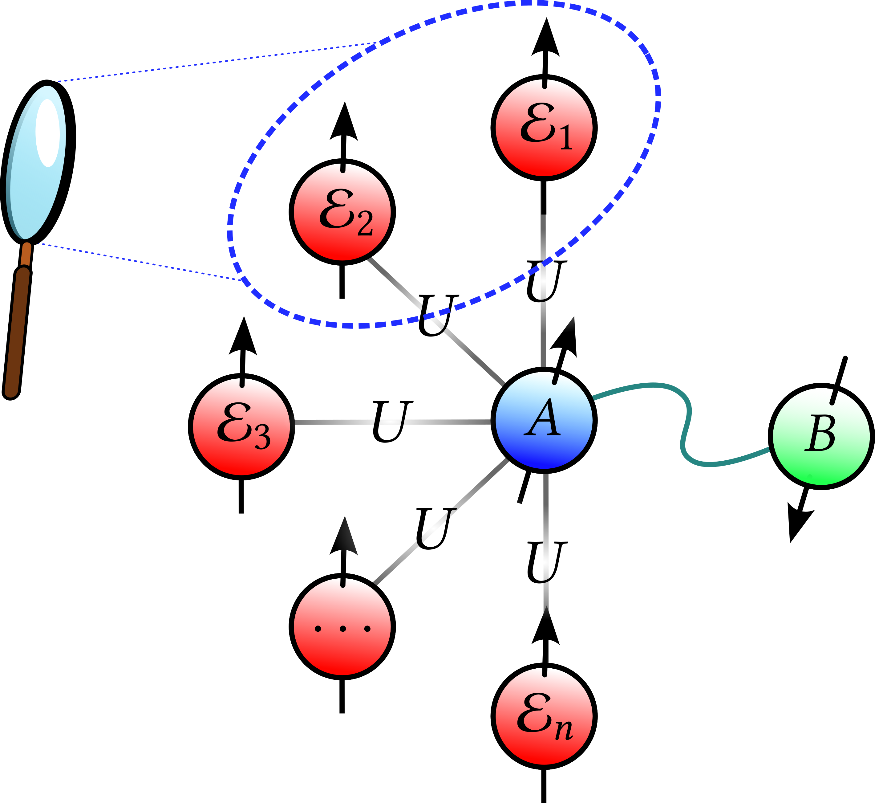
Figure 1: A bipartite system $\rho_{\mathcal{AB}}$ with arbitrary dimension is monitored by a collection of environmental subsystems $\{\mathcal{E}_{i}\}_{i=1}^{n}$, with each interaction represented by a unitary evolution acting on the joint system. The interaction with the environment establishes not just the realism associated with the context $\{A,\rho_{\mathcal{AB}}\}$, but also the proliferation of redundant information about the system in small portions of the environment; a key process in Quantum Darwinism. This proliferation of redundant information can be associated with the emergence of objective reality since several observers will agree on their outcomes after accessing the information about the system that is encoded in the environment.

In this work, we propose to establish the connection between quantum irrealism and quantum Darwinism for discrete quantum systems with higher dimensions. As a starting point, we discuss the qubit regime and address its limitations as well as its direct generalizations. After that, to address the qudit regime, we will model the interaction between the system and the environment through generalized observables [21], described by the Fourier transform of POVMs, which allow the control of their disturbance on the measured quantum system, therefore, allowing an interpolation from a weak to strong projective action [22, 10]. This interpolation regime was experimentally investigated for qubits employing a trapped-ion platform [23], and with photonic weak measurements [18]. In Fig. 1 we give a depiction of the scenario we are modeling.

Irrealism.— The quantum realism argument can be formalized as follows. Let $A=\sum_{a}aA_{a}$ be a $d$-output observable acting on $\mathcal{H_{A}}$, where $A_{a}={|{a}\rangle}\!{\langle{a}|}$ are projectors satisfying $\sum_{a}A_{a}=\mathbbm{1}_{\mathcal{A}}$. Also, let $\Phi_{A}(\varrho)=\sum_{a}(A_{a}\otimes\mathbbm{1}_{\mathcal{B}})\varrho(A_{a}\otimes\mathbbm{1}_{\mathcal{B}})$ be the non-selective projective measurement of the observable $A$. A bipartite system $\rho_{\mathcal{AB}}$ acting over $\mathcal{H}_{\mathcal{AB}}$ is said to have realism defined for the observable $A$ acting on $\mathcal{H_{A}}$ iff

$$\Phi_{A}(\rho_{\mathcal{AB}})=\rho_{\mathcal{AB}}.$$ (1)

States that already have realism defined for some observable are invariant to a non-selective (or non-revealed) projective measurement of the same observable, i.e. $\Phi_{A}(\Phi_{A}(\rho))=\Phi_{A}(\rho)$. Subsequently, the irreality of $A$ given $\rho$

$$\mathfrak{I}_{A}(\rho)\coloneqq\min_{\varrho}S\big{(}\rho||\Phi_{A}(\varrho)\big{)}=S\big{(}\Phi_{A}(\rho)\big{)}-S(\rho)$$ (2)

proved to be a faithful quantifier of $A$-realism violations for a given state $\rho$ [17, 10, 20], where $S(\rho||\sigma)=\Tr[\rho(\log_{2}{\rho}-\log_{2}{\sigma})\big{]}$ stands for the relative entropy and $S(\rho)\coloneqq\text{Tr}\big{(}\rho\log_{2}{\rho}\big{)}$ is the von Neumann entropy. In addition, we can decompose irreality as local coherence plus non-optimized quantum discord, i.e. $\mathfrak{I}_{A}(\rho)=\mathcal{C}(\rho_{\mathcal{A}})+D_{A}(\rho)$ where $\mathcal{C}(\rho_{\mathcal{A}})=\mathfrak{I}_{A}(\Tr_{\mathcal{B}}\rho)$, $D_{A}(\rho)=I_{\mathcal{A:B}}(\rho)-I_{\mathcal{A:B}}(\Phi_{A}(\rho))$, and $I_{\mathcal{A:B}}=S(\rho_{\mathcal{A}})+S(\rho_{\mathcal{B}})-S(\rho_{\mathcal{AB}})$ is the quantum mutual information. Consequently, correlations between parties $\mathcal{A}$ and $\mathcal{B}$ prevent the existence of elements of physical reality for observables on both parties, that is, any positive value for $D_{A(B)}(\rho)$ implies non-null irrealism $\mathfrak{I}_{A(B)}(\rho)\geq 0$

The irrealism measure was theoretically employed to study a series of foundational problems [24, 25, 26, 27, 28, 29, 30, 20, 31, 32]. Moreover, some experimental reports include: a nuclear magnetic resonance experiment to probe the robustness of the wave-particle duality in a quantum-controlled interferometer [33], and photonic [18] and superconducting qubits [34] to investigate the emergence of realism upon monitoring maps [10, 35]. Such maps are defined as

$$\mathcal{M}_{A}^{\epsilon}(\varrho)\coloneqq(1-\epsilon)\rho+\epsilon\Phi_{A}(\varrho),$$ (3)

that is, an interaction that produces as an output an interpolation between the weak and strong non-selective measurement regimes for the measured system.

Qubit case.— Now, let us describe the monitoring map from the point of view of the global interaction between the system and the environment. The simplest model describing a measurement procedure is constituted by a single CNOT gate. Suppose that our system of interest $\mathcal{S}$ is composed of only one arbitrary qubit in the state $\rho_{\mathcal{S}}$, but the environment $\mathcal{E}$ is known to be $\rho_{\mathcal{E}}={|{0}\rangle}\!{\langle{0}|}$. A CNOT gate, which can be written in the form [36]

$$U_{\textrm{CNOT}}={|{0}\rangle}\!{\langle{0}|}\otimes\mathbbm{1}+{|{1}\rangle}\!{\langle{1}|}\otimes\sigma_{x},$$ (4)

keeps the qubit in the environment in the same state if the state of the system is ${|{0}\rangle}$ and flips it if the state is ${|{1}\rangle}$. Contrary to the classical notion, if the system lies in a superposition, such a superposition will be extended to the environment in the form of entanglement. Indeed, the global state $\Omega\coloneqq\rho_{\mathcal{S}}\otimes{|{0}\rangle}\!{\langle{0}|}$ evolves to

$$\Omega^{\prime}\coloneqq U\Omega U^{\dagger}=\sum_{i,j=0}^{1}{\langle{i}|}\rho_{\mathcal{S}}{|{j}\rangle}\ {|{i}\rangle}\!{\langle{j}|}\otimes{|{i}\rangle}\!{\langle{j}|}.$$ (5)

Now, if we discard the information in the environment by tracing it out, the resulting operation over the system is a non-selective measurement in the form of

$$\Tr_{\mathcal{E}}\Omega^{\prime}=\sum_{i\,=\,0}^{1}{\langle{i}|}\rho_{\mathcal{S}}{|{i}\rangle}\ {|{i}\rangle}\!{\langle{i}|}=\Phi_{\sigma_{z}}(\rho_{\mathcal{S}}),$$ (6)

where $\sigma_{z}={|{0}\rangle}\!{\langle{0}|}-{|{1}\rangle}\!{\langle{1}|}$. The map $\Phi_{\sigma_{z}}$ above means that a measurement in the $z$ direction was realized, but the outcome was not recorded; a sufficient condition for the establishment of realism for observable $\sigma_{z}$. Since (5) is symmetric, we have that $\Tr_{\mathcal{S}}\Omega^{\prime}=\Tr_{\mathcal{E}}\Omega^{\prime}$, and thus the probability $p_{i}=\Tr({|{i}\rangle}\!{\langle{i}|}\rho_{\mathcal{S}})$ is now encoded in the environment. It turns out that, in a practical situation, this is not always the case, as the CNOT gate cannot be perfectly implemented due to operational errors. Thus, only partial information regarding the observable can be retrieved; which, however, can be circumvented by interacting the system with more qubits in the environment to create redundant accessible information, following the Quantum Darwinism framework.

One way to model a noisy CNOT gate for qubits was explored in Ref. [13] by simply replacing the $\sigma_{x}$ operator in $U_{\textrm{CNOT}}$ with the unitary $\sigma_{\theta}$, which is defined as a linear combination $\sigma_{\theta}\coloneqq\cos\theta\sigma_{x}+\sin\theta\sigma_{z}$. In this letter, we show that by controlling the interaction intensity between the system and the single environmental qubit through the parameter $\theta$, we can interpolate between weak and strong projective non-selective measurements. In detail, a noisy $U_{\textrm{CNOT}}$ with $\sigma_{\theta}$ results in a monitoring map $\mathcal{M}_{A}^{\epsilon}$ after tracing out the environment (see Sec. B in the Supplemental Material). However, since this procedure only applies to qubit systems, it is very likely not a good model for more complex systems. By restricting ourselves to only two dimensions we may miss certain effects which appear only for high dimensional systems. Therefore, our motivation in this letter is to find such a model for arbitrary local dimensions. To this end, we need to find a unitary operation acting on qudits that can be adjusted to interpolate between weak and strong non-selective measurement regimes.

Generalized observables.— One way to generalize $U_{\textrm{CNOT}}$ for qudits (including the noisy regime) is to replace the Pauli operators with the Heisenberg-Weyl operators

$$Z=\sum_{k\,=\,0}^{d-1}\omega^{k}{|{k}\rangle}\!{\langle{k}|},\qquad X=\sum_{k\,=\,0}^{d-1}{|{k+1}\rangle}\!{\langle{k}|},$$ (7)

where ${|{d}\rangle}\equiv{|{0}\rangle}$, $\omega=e^{2\pi\mathbbm{i}/d}$ is the complex root of unity, and $d=\dim\mathcal{H}$ is the dimension of the Hilbert space. It can be verified that $X^{\dagger}X=Z^{\dagger}Z=\mathbbm{1}_{\mathcal{H}}$, $X^{d}=Z^{d}=\mathbbm{1}_{\mathcal{H}}$, and $Z^{l}X^{k}=\omega^{lk}X^{k}Z^{l}$. Also, when $d=2$, then $Z$ and $X$ are the usual $\sigma_{z}$ and $\sigma_{x}$ Pauli matrices, respectively. Thus, $\sigma_{\theta}$ becomes $\cos\theta X+\sin\theta Z\eqqcolon T$ and then we can take its powers:

$$U_{\textrm{noisy CNOT}}={|{0}\rangle}\!{\langle{0}|}\otimes\mathbbm{1}+{|{1}\rangle}\!{\langle{1}|}\otimes T+{|{2}\rangle}\!{\langle{2}|}\otimes T^{2}+\ldots.$$ (8)

The problem is: it is impossible to obtain a unitary operator as a linear combination of only $X$ and $Z$ for $d\geqslant 3$ [21, 37]. Nonetheless, one can always find a linear combination of $\{XZ^{k}\}$ or $\{ZX^{k}\}$ for $k\,=\,0,\ldots,d-1$ that results in a unitary operator.

Although $Z$ contains complex eigenvalues, it can fully characterize a valid observable as well as $X$. More generally, let us consider a $d$-outcome quantum measurement $M=\{M_{a}\}$ which is defined by positive-semidefinite operators $M_{a}$ acting on a Hilbert space $\mathcal{H}$, such that $\dim\mathcal{H}=d$ and $\sum_{a}M_{a}=\mathbbm{1}_{\mathcal{H}}$. The measurement $M$ is simply a POVM, but if $M_{a}M_{a^{\prime}}=\delta_{aa^{\prime}}M_{a}$, then $M$ is a projective measurement. For qudits, it is convenient to use generalized observables by taking a discrete Fourier transform of $M$

$$F^{(i)}=\sum_{a\,=\,0}^{d-1}\omega^{ia}M_{a},$$ (9)

Immediately, $F^{(0)}=\mathbbm{1}_{\mathcal{H}}$. By performing the inverse Fourier transform on the generalized observables $F^{(i)}$, one can recover the measurement $M$

$$M_{a}=\dfrac{1}{d}\sum_{i\,=\,0}^{d-1}\omega^{-ia}F^{(i)}.$$ (10)

Therefore, the generalized observables $F^{(i)}$ fully characterize the measurement $M$. In addition, the POVM $\{M_{a}\}$ is a projective measurement iff $F\coloneqq F^{(1)}$ is the identity. In that case, $F$ is called the unitary observable of $\{M_{a}\}$ and $F^{(i)}=F^{i}$ (see Ref. [21] for detailed proofs).

Results.— Consider the scenario depicted in Fig. 1. Let $\mathcal{H=H_{S}}\otimes\mathcal{H_{E}}$, where $\mathcal{S}$ and $\mathcal{E}$ stand for system and environment, respectively, such that $\mathcal{H_{S}}=\mathcal{H_{A}\otimes H_{B}}$ and $\mathcal{H_{E}}=\bigotimes_{k=1}^{n}\mathcal{H}_{\mathcal{E}_{k}}$, with party $\mathcal{A}$ containing one qudit and party $\mathcal{E}$ containing $n$ qudits. Note that the fragment $\mathcal{F}_{m}$ of the environment $\mathcal{E}$ is constituted by $\mathcal{H}_{\mathcal{F}_{m}}=\bigotimes_{k=1}^{m}\mathcal{H}_{\mathcal{E}_{k}}$, with $m\leqslant n$. For our purposes, it is important to consider that $\dim\mathcal{H_{A}}=\dim\mathcal{H}_{\mathcal{E}_{i}}\eqqcolon d$ for all $i$.

We propose a noisy CNOT gate $U_{\mathcal{SE}_{i}}$ that acts over $\mathcal{H}_{\mathcal{AE}_{i}}$, which entangles the qudit of the system with qudit $i$ in the environment, and it is defined as

$$U_{\mathcal{SE}_{i}}\coloneqq\sum_{j\,=\,0}^{d-1}P_{j}\otimes T^{j},$$ (11)

where $P_{j}=A_{j}\otimes\mathbbm{1}_{\mathcal{B}}$ is the projector acting on subspace $\mathcal{H}_{\mathcal{S}}$ and $T$ is a unitary observable given by

$$T\coloneqq\sum_{k\,=\,0}^{d-1}\alpha_{k}ZX^{k},\qquad\alpha_{k}=\dfrac{1}{d}\sum_{l\,=\,0}^{d-1}\omega^{-lk}e^{\mathbbm{i}\phi_{l}},$$ (12)

with the conditions $\phi_{0}=\theta$, $\phi_{1}=-\theta$, and $\phi_{k\geqslant 2}\,=\,0$. Note that $U_{\mathcal{SE}_{i}}$ follows the same structure as Eq. (8), but now $T^{\dagger}T=\mathbbm{1}_{\mathcal{E}}$, which guarantees unitarity of $U_{\mathcal{SE}_{i}}$, and $T^{d}=\mathbbm{1}_{\mathcal{E}}$, which guarantees the correct spectrum (see Sec. C in the Supplemental Material for proofs). More importantly than that, operator $T$ does not depend on the choice of $A$, that is, $A$ is an arbitrary measurement and $T$ is just a way to encode information about the system in the environment. One can also show that

$$\alpha_{k}=\left\{\begin{array}[]{ll}1-\dfrac{2}{d}(1-\cos\theta),&\textrm{if }k\,=\,0,\\ \dfrac{1}{d}\left(e^{i\theta}+e^{-i\theta}\omega^{-k}-1-\omega^{-k}\right),&\textrm{if }1\leqslant k\leqslant d-1,\end{array}\right.$$ (13)

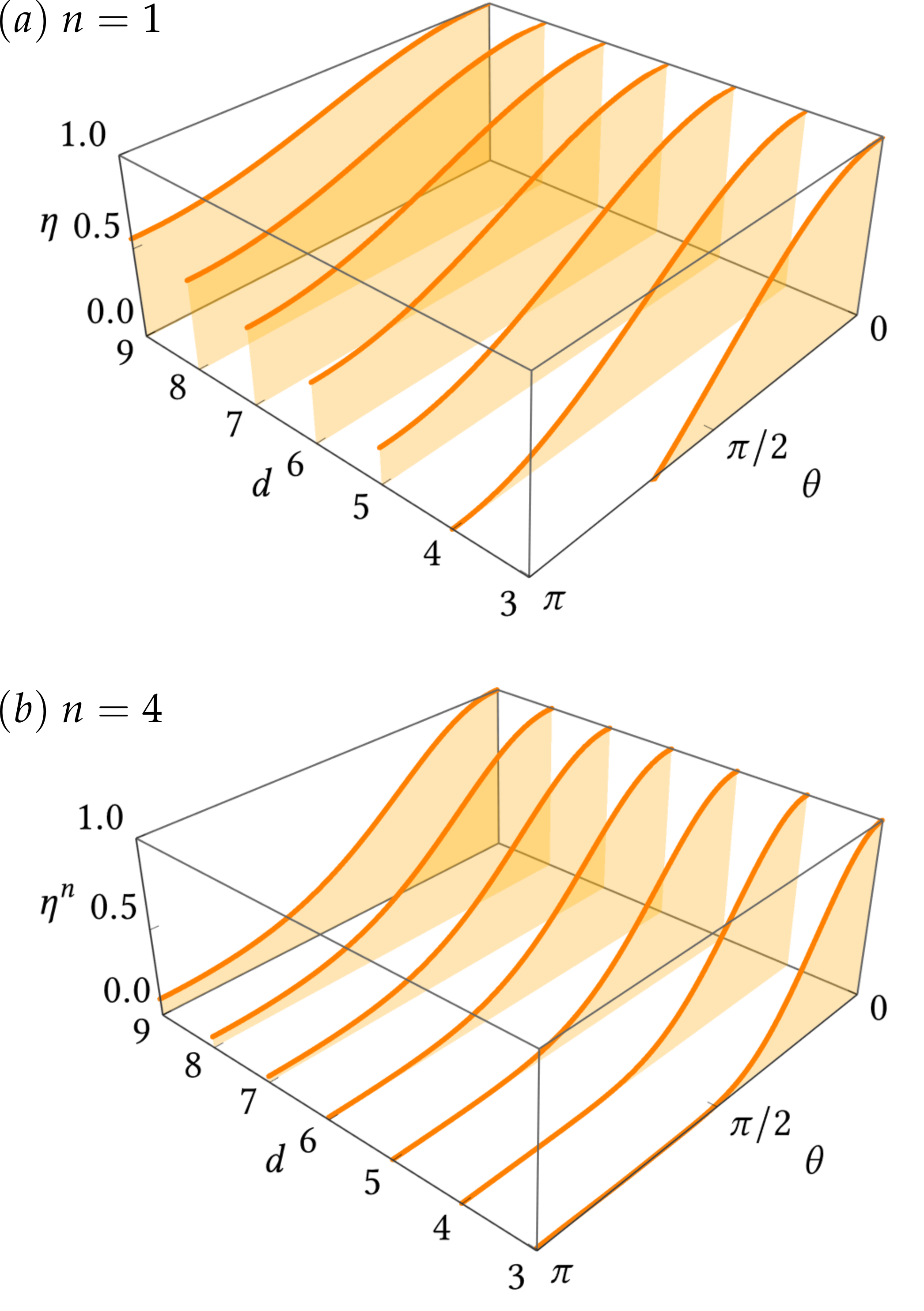
Figure 2: $(a)$ Noise $\eta$ as a function of $d$ and $\theta$. If the environment is composed of only one qudit, then zero noise scenario, i.e. strong non-selective measurement, can be achieved only for dimensions $d=3$ and $4$. $(b)$ Effective noise $\eta^{n}$ for $n=4$ as a function of $d$ and $\theta$. By adding more qudits in the environment, the effective noise can be reduced as much as we wish.

and that $\sum_{k\,=\,0}^{d-1}|\alpha_{k}|^{2}=1$. It is important to keep in mind that, given $d$, the parameter $\theta$ must be such that $0\leqslant\alpha_{0}\leqslant 1$. Without loss of generality, we can suppose that every qudit in the environment is in the state ${|{0}\rangle}_{\mathcal{E}_{i}}$ being ready to receive information about the system of interest. To make things easier to follow, let us begin with the interaction between the system and the first qudit in the environment given by $\rho_{\mathcal{SE}_{1}}^{\prime}\coloneqq U_{\mathcal{SE}_{1}}\rho_{\mathcal{SE}_{1}}U_{\mathcal{SE}_{1}}^{\dagger}$, where $\rho_{\mathcal{SE}_{1}}=\rho_{\mathcal{AB}}\otimes{|{0}\rangle}\!{\langle{0}|}_{\mathcal{E}_{1}}$. After applying (11) in the above expression and tracing out the first environment we get

$$\Tr_{\mathcal{E}_{1}}\rho_{\mathcal{SE}_{1}}^{\prime}=\sum_{i,j\,=\,0}^{d-1}P_{i}\rho P_{j}{\langle{0}|}(T^{j})^{\dagger}T^{i}{|{0}\rangle}_{\mathcal{E}_{1}}$$ (14)

After some algebra (see Sec. C in the Supplemental Material), it is possible to verify that

$${\langle{0}|}(T^{j})^{\dagger}T^{i}{|{0}\rangle}_{\mathcal{E}_{1}}=\eta+\delta_{i,j}(1-\eta),$$ (15)

where $\eta\coloneqq\alpha_{0}$ and $i,j\,=\,0,\ldots,d-1$. By plugging the above in Eq. (14) and using the definition of monitoring (3), it is possible to show that (see Sec. D in the Supplemental Material)

$$\Tr_{\mathcal{E}_{1}}\rho_{\mathcal{SE}_{1}}^{\prime}=\mathcal{M}_{A}^{\epsilon=1-\eta}(\rho_{\mathcal{AB}}),$$ (16)

where we can see now that $\eta$ can be interpreted as the level of noise in the measurement; the complement of the monitoring intensity $\epsilon$. In Fig. 2 $(a)$ we can see how the noise depends on the parameter $\theta$ and the dimension $d$ of the system being measured.

Eq. (16) is our first main result. It shows that the noisy CNOT gate (11) provides the monitoring map (3) after we trace out the environment. Because of the Stinespring dilation theorem [38, 36], the unitary operator that provides the map $\mathcal{M}_{A}^{\epsilon}$ after the partial trace must be unique, up to local isometries. However, from Fig. 2 $(a)$ we can see that, within our model, we can only perform strong (projective, i.e. $\eta\,=\,0$) measurements over the system when the qudit of interest has dimension $d=3$ or $4$. For $d\geqslant 5$, only partial information (i.e. $\eta>0$) can be retrieved from the system by accessing the environment; which makes sense from the physical point of view since the bigger the dimension, the easier to occur decoherence.

The natural question to do now is how to obtain full information about the system by using gate (11). We are going to show that to obtain full information we need a bigger environment, i.e. more qudits. As pictured in Fig. 1, let us define the global unitary that will perform the interaction between the system with the entire environment $U\coloneqq U_{\mathcal{SE}_{n}}\ldots U_{\mathcal{SE}_{1}}$. The initial global state of the system+environment is given by $\Omega\coloneqq\rho_{\mathcal{AB}}\otimes\bigotimes_{i=1}^{n}{|{0}\rangle}\!{\langle{0}|}_{\mathcal{E}_{i}}$. After the unitary evolution $\Omega^{\prime}\coloneqq U\Omega U^{\dagger}$, we can write

$$\Omega^{\prime}=\sum_{i,j\,=\,0}^{d-1}P_{i}\rho P_{j}\otimes\bigotimes_{k=1}^{n}T_{i}{|{0}\rangle}\!{\langle{0}|}_{\mathcal{E}_{k}}(T_{j})^{\dagger}.$$ (17)

If we trace out the whole environment, the remaining state of the system will be given by (see Sec. D in the Supplemental Material)

$$\Tr_{\mathcal{E}}\Omega^{\prime}=\mathcal{M}_{A}^{1-\eta^{n}}(\rho_{\mathcal{AB}}).$$ (18)

Now, we can apply Eq. (18) from Ref. [10], i.e.,

$$\left[\mathcal{M}_{A}^{\epsilon}\right]^{n}(\rho_{\mathcal{AB}})=\mathcal{M}_{A}^{1-(1-\epsilon)^{n}}(\rho_{\mathcal{AB}})$$ (19)

to Eq. (18) to obtain

$$\Tr_{\mathcal{E}}\Omega^{\prime}=\left[\mathcal{M}_{A}^{\epsilon=1-\eta}\right]^{n}(\rho_{\mathcal{AB}}).$$ (20)

The Eq. (18) is our second main result. It shows that subsequent interactions between the system and $n$ environmental qudits through the noisy CNOT gate (11) result in a monitoring map of intensity $1-\eta^{n}$, which allows us to interpret $\eta^{n}$ as the effective noise. In Fig. 2 $(b)$, we can see how the effective noise is suppressed by adding more environmental qudits. In addition, from Eq. (20), we can see that each weak interaction with some part of the environment produces one more monitoring over the system. This process clearly decreases the degree of irreality (2) and makes the system more classical regarding observable $A$ [29, 20].

Immediately, from (18) and the definition of a monitoring, we have

$$\lim_{n\to+\infty}\left(\Tr_{\mathcal{E}}\Omega^{\prime}\right)=\Phi_{A}(\rho_{\mathcal{AB}}).$$ (21)

From the information-realism complementarity (originally in Ref. [10], but revisited in Sec. A of the Supplemental Material), we can conclude another significant result. In practical terms, equation (21) means that in order to codify the total accessible quantum information regarding the observable $A$ of a higher dimensional system into the environment, it is necessary to make the system interact several times with the environment. From another perspective, we can also infer from our model that in more complex systems, states of reality $\Phi_{A}(\rho)$ can only be achieved by making the system interact with more fragments of the environment, in agreement with the quantum Darwinistic perspective. In that sense, this model suggests that nature imposes restrictions on how the information can be redundantly codified in the environment; if the system is too complex (high-dimensional) we cannot codify all the information related with some observable into a unique environmental qudit, but rather into multiple qudits

To this end, let us consider the noisy CNOT gate $U_{\mathcal{SE}_{i}}$ given by Eq. (11) for dimension $d=2$, i.e. $U_{\mathcal{SE}_{i}}={|{0}\rangle}\!{\langle{0}|}\otimes\mathbbm{1}+{|{1}\rangle}\!{\langle{1}|}\otimes T$, where $T=-\sin\theta\sigma_{y}+\cos\theta\sigma_{z}$ is given by Eq. (28). The resulting monitoring map will have intensity $\epsilon=1-\cos\theta$, reproducing the effects of the c-maybe gate from the work of Touil et al. [13], up to a $\pi/2$ phase on $\theta$ (see Sec. B in the Supplemental Material).

Conclusion.— Irrealism can be framed as a resource [29], has an intimate connection with the concept of information [10, 20], and monitoring is identified as a realistic operation, meaning that in general the irrealism of the context $\{A,\rho_{\mathcal{AB}}\}$ is destroyed by $A$-monitorings [10] via the flow of information between the system and the auxiliary system.

In this work, we take a step further in such connections by demonstrating that, within our model, finite higher dimensional monitoring necessarily requires multiple environmental qudits, which means that the emergence of realism for a generic observable $A$ can only be gradually tuned in the form of interpolation between weak and strong regimes by the action of multiple interactions. This condition unveils a new connection between two different concepts, namely, irrealism and quantum Darwinism. Increasing the dimension of the system of interest also means increasing the number of environmental systems required to obtain total accessible quantum information about the observable of interest. This suggests that redundant information is an important ingredient to establishing realism for such systems which also implies an objective reality as the one given when redundant information is proliferated to the environment.

Further connections can be done by exploring this new relation, for instance, by analyzing how the information-reality complementarity relates to the presence of redundant information and the necessity of more than one auxiliary system to perform the interpolation. Also, this framework sheds new light on long-debated problems such as the one related to the notion of measurement in quantum theory with the identification that the gradual emergence of realism for qudits asks for multiple informers.

SUPPLEMENTAL MATERIAL

Appendix A Information-realism complementarity

Consider the amount of accessible information of a generic quantum state $\rho$ in a Hilbert space $\mathcal{H_{S}}$ with dimension $d$ as

$$I(\rho):=\ln{d}-S(\rho).$$ (22)

Following Ref. [10], wherein a complementarity relation between information and the degree of irrealism for some discrete observable was introduced, we can check that

$$[\mathcal{M}_{A}^{\epsilon}]^{n}\big{(}\Phi_{A}(\rho)\big{)} =(1-\epsilon)^{n}\Phi_{A}(\rho)+\big{[}1-(1-\epsilon)^{n}\big{]}\Phi_{A}(\rho)$$ (23)

$$=\Phi_{A}(\rho)=\Phi_{A}\big{(}\mathcal{M}_{\epsilon,A}^{n}(\rho)\big{)}.$$

which proves the hierarchy of the map $\Phi_{A}$ over $[\mathcal{M}_{A}^{\epsilon}]^{n}$. Interestingly, this shows that the map $\mathcal{M}_{A}^{\epsilon}$ commutes with the map $\Phi_{A}$ for all intensities $\epsilon$. Employing entropy concavity and the non-negativity of the irrealism measure $\mathfrak{I}_{A}(\rho)$, we can evaluate the difference in the irrealism given monitoring of the same observable

$$\Delta\mathfrak{I}_{A}:=\mathfrak{I}_{A}(\rho)-\mathfrak{I}_{A}(\mathcal{M}_{A}^{\epsilon}(\rho))=S\left(\mathcal{M}_{A}^{\epsilon}(\rho)\right)-S(\rho)\geqslant\epsilon\mathfrak{I}_{A}(\rho),$$ (24)

equality for $\epsilon=0$. Introducing the amount of remaining accessible information after some monitoring of a generic observable $A$ as

$$\Delta I_{\mathcal{S}}:=I(\rho)-I(\mathcal{M}_{A}^{\epsilon}(\rho))=S\left(\mathcal{M}_{A}^{\epsilon}(\rho)\right)-S(\rho)=\Delta\mathfrak{I}_{A},$$ (25)

which means that the irrealism of the observable $A$ for the preparation $\rho$ quantifies the amount of remaining accessible information that still can be extracted after a weak non-selective measurement of $A$. It is important to note that either when $\epsilon=1$ or when $\lim_{n\to+\infty}[\mathcal{M}_{A}^{\epsilon}]^{n}$ for infinitely successive applications, $\mathfrak{I}_{A}(\rho)=\Delta I_{\mathcal{S}}$.

Moreover, one can prove that the information flow between the system $\mathcal{H_{S}}$ and the total environment $\mathcal{H_{E}}$ when we impose a global unitary dynamics that reproduces the monitoring of $A$ is

$$\Delta\mathfrak{I}_{A}=\Delta(I_{\mathcal{S:E}}+I_{\mathcal{E}}),$$ (26)

where $I_{\mathcal{S:E}}(\rho)=S(\rho_{\mathcal{S}})+S(\rho_{\mathcal{E}})-S(\rho)$ stands for the quantum mutual information. In other words, because the environment $\mathcal{E}$ gets information about $A$, this observable increases its realism degree. In the limit of strong non-selective measurements, irrealism goes to zero as well as the accessible information about this observable.

The same rationale can be employed in our model as the noisy CNOT gate $U_{\mathcal{SE}_{i}}$ that acts over $\mathcal{H}_{\mathcal{AE}_{i}}$, which entangles the qudit of the system with qudit $i$ in the environment via the unitary coupling

$$U_{\mathcal{SE}_{i}}=\sum_{j\,=\,0}^{d-1}P_{j}\otimes T^{j},$$ (27)

where $P_{j}=A_{j}\otimes\mathbbm{1}_{\mathcal{B}}$ is the projector acting on subspace $\mathcal{H}_{\mathcal{S}}$ and $T$ is a unitary observable given by

$$T=\sum_{k\,=\,0}^{d-1}\alpha_{k}ZX^{k},\qquad\alpha_{k}=\dfrac{1}{d}\sum_{l\,=\,0}^{d-1}\omega^{-lk}e^{\mathbbm{i}\phi_{l}},$$ (28)

with the conditions $\phi_{0}=\theta$, $\phi_{1}=-\theta$, and $\phi_{k\geqslant 2}\,=\,0$. As we proved in the manuscript, the following relation holds for every dimension $d$

$$\lim_{n\to+\infty}\left(\Tr_{\mathcal{E}}\Omega^{\prime}\right)=\Phi_{A}(\rho_{\mathcal{S}}),$$ (29)

which means that the whole effective environment has now access to the full information about the observable $A$ for the quantum system $\rho$, as demonstrated by the relation $I(\rho)-I(\Phi_{A}(\rho))=\mathfrak{I}_{A}(\rho)$.

Appendix B Qubit case — the c-maybe gate

Let us consider the c-maybe gate [13]

$$U_{\oslash}\coloneqq{|{0}\rangle}\!{\langle{0}|}\otimes\mathbbm{1}+{|{1}\rangle}\!{\langle{1}|}\otimes\sigma_{\theta}=\sum_{k=0}^{1}P_{k}\otimes\sigma_{\theta}^{k},$$ (30)

where $\sigma_{\theta}\coloneqq\cos\theta\sigma_{x}+\sin\theta\sigma_{z}$ acts over $\mathcal{H}_{\mathcal{E}_{1}}$ and $P_{k}=A_{k}\otimes\mathbbm{1}_{\mathcal{B}}$ are projectors in $\mathcal{H}_{\mathcal{S=AB}}$ s.t. $A=\sum_{k}a_{k}A_{k}$ is the observable of interest in $\mathcal{H_{A}}$, $A_{k}A_{k^{\prime}}=\delta_{kk^{\prime}}A_{k}$, and $\sum_{k}A_{k}=\mathbbm{1}_{\mathcal{A}}$. It can be checked that

$${\langle{0}|}\sigma_{\theta}^{i}\sigma_{\theta}^{j}{|{0}\rangle}=\sin\theta+\delta_{i,j}(1-\sin\theta),$$ (31)

for $i,j=0,1$. If the initial state of the global system is given by two qubits in the state $\rho_{\mathcal{S}\mathcal{E}_{1}}=\rho_{\mathcal{AB}}\otimes{|{0}\rangle}\!{\langle{0}|}_{\mathcal{E}_{1}}$, then the evolved state is

$$\rho_{\mathcal{S}\mathcal{E}_{1}}^{\prime}\coloneqq U_{\oslash}\rho_{\mathcal{S}\mathcal{E}_{1}}U_{\oslash}^{\dagger}=\sum_{i,j=0}^{1}P_{i}\rho_{\mathcal{AB}}P_{j}\otimes\sigma_{\theta}^{i}{|{0}\rangle}\!{\langle{0}|}_{\mathcal{E}_{1}}(\sigma_{\theta}^{j})^{\dagger}.$$ (32)

If we trace out the environmental qubit, we obtain

$$\Tr_{\mathcal{E}_{1}}\left(\rho_{\mathcal{S}\mathcal{E}_{1}}^{\prime}\right)=\sum_{i,j=0}^{1}P_{i}\rho_{\mathcal{AB}}P_{j}{\langle{0}|}(\sigma_{\theta}^{j})^{\dagger}\sigma_{\theta}^{i}{|{0}\rangle}_{\mathcal{E}_{1}}=\sum_{i,j=0}^{1}P_{i}\rho_{\mathcal{AB}}P_{j}[\sin\theta+\delta_{i,j}(1-\sin\theta)],$$ (33)

which can be written as

$$\Tr_{\mathcal{E}_{1}}\left(\rho_{\mathcal{S}\mathcal{E}_{1}}^{\prime}\right)=\sin\theta\sum_{i,j=0}^{1}P_{i}\rho_{\mathcal{AB}}P_{j}+(1-\sin\theta)\sum_{i=0}^{1}P_{i}\rho_{\mathcal{AB}}P_{i}=\sin\theta\rho_{\mathcal{AB}}+(1-\sin\theta)\Phi_{A}(\rho_{\mathcal{AB}}).$$ (34)

By the definition of a monitoring map

$$\mathcal{M}_{A}^{\epsilon}(\varrho)\coloneqq(1-\epsilon)\rho+\epsilon\Phi_{A}(\varrho),$$ (35)

we have that

$$\Tr_{\mathcal{E}_{1}}\left(\rho_{\mathcal{S}\mathcal{E}_{1}}^{\prime}\right)=\mathcal{M}_{A}^{1-\sin\theta}(\rho_{\mathcal{AB}}).$$ (36)

As we can see here, the c-maybe operator written in the eigenbasis of $A$ is precisely the unitary evolution, up to local isometries, that results in a monitoring of $A$ with intensity $\epsilon=1-\sin\theta$ after we trace out the environment.

Appendix C Properties of operator $T$

Consider the unitary observable $T$ given by

$$T\coloneqq\sum_{k\,=\,0}^{d-1}\alpha_{k}ZX^{k},\qquad\alpha_{k}=\dfrac{1}{d}\sum_{l\,=\,0}^{d-1}\omega^{-lk}e^{\mathbbm{i}\phi_{l}}.$$ (37)

Imposing the conditions $\phi_{0}=\theta$, $\phi_{1}=-\theta$, and $\phi_{k\geqslant 2}\,=\,0$, we have

$$\alpha_{0}=\frac{1}{d}\sum_{l\,=\,0}^{d-1}e^{\mathbbm{i}\phi_{l}}=\frac{e^{i\theta}+e^{-i\theta}+d-2}{d}=1-\dfrac{2}{d}(1-\cos\theta),$$ (38)

and

$$\alpha_{k}=\dfrac{1}{d}\left(e^{i\theta}+e^{-i\theta}\omega^{-k}-1-\omega^{-k}\right),\quad\textrm{for }k=1,\ldots,d-1.$$ (39)

Now, let us prove three essential properties of the operator $T$.

Proposition 1.

The operator $T$ is unitary.

Proof.

Explicitly,

$$TT^{\dagger}=\left(\sum_{k\,=\,0}^{d-1}\alpha_{k}ZX^{k}\right)\left(\sum_{q\,=\,0}^{d-1}\alpha_{q}^{*}X^{-q}Z^{-1}\right).$$ (40)

By performing the products, we obtain

$$TT^{\dagger}=\sum_{k\,=\,0}^{d-1}|\alpha_{k}|^{2}\mathbbm{1}+\sum_{\begin{subarray}{c}k,q\,=\,0\\ k\neq q\end{subarray}}^{d-1}\alpha_{k}\alpha_{q}^{*}ZX^{k-q}Z^{-1}.$$ (41)

For simplicity, let us denote $n\coloneqq k-q$ and rewrite the above in the following form

$$TT^{\dagger}=\sum_{k\,=\,0}^{d-1}|\alpha_{k}|^{2}\mathbbm{1}+\sum_{n=1}^{d-1}\sum_{q\,=\,0}^{d-1}\alpha_{n+q}\alpha_{q}^{*}ZX^{n}Z^{-1}.$$ (42)

Let us start by developing the first sum in the r.h.s. of the above expression:

$$\sum_{k\,=\,0}^{d-1}|\alpha_{k}|^{2}=\sum_{k\,=\,0}^{d-1}\dfrac{1}{d^{2}}\left(e^{\mathbbm{i}\theta}+\omega^{-k}e^{-\mathbbm{i}\theta}+\sum_{m_{1}=2}^{d-1}\omega^{-km_{1}}\right)\left(e^{-\mathbbm{i}\theta}+\omega^{k}e^{\mathbbm{i}\theta}+\sum_{m_{2}=2}^{d-1}\omega^{km_{2}}\right).$$ (43)

From the identity

$$\sum_{k\,=\,0}^{d-1}\omega^{(a-b)k}=d\delta_{a,b},$$ (44)

where $a$ and $b$ are any integers and

$$\delta_{a,b}\coloneqq\begin{cases}1&\textrm{for }a=b\mod d,\\ 0&\textrm{for }a\neq b\mod d,\end{cases}$$ (45)

we can compute the r.h.s of (43) and reach

$$\sum_{k\,=\,0}^{d-1}|\alpha_{k}|^{2}=1.$$ (46)

Now, let us show that the second sum in the r.h.s. of (42) will vanish. Indeed,

$$\sum_{q\,=\,0}^{d-1}\alpha_{n+q}\alpha_{q}^{*}=\sum_{q\,=\,0}^{d-1}\dfrac{1}{d^{2}}\left(e^{\mathbbm{i}\theta}+\omega^{-n-q}e^{-\mathbbm{i}\theta}+\sum_{m_{1}=2}^{d-1}\omega^{-m_{1}(n+q)}\right)\left(e^{-\mathbbm{i}\theta}+\omega^{q}e^{\mathbbm{i}\theta}+\sum_{m_{2}=2}^{d-1}\omega^{m_{2}q}\right),$$ (47)

which by implementing identity (44) multiple times results in

$$\sum_{q\,=\,0}^{d-1}\alpha_{n+q}\alpha_{q}^{*}\,=\,0.$$ (48)

Putting (46) and (48) in (42) gives the desired result. ∎

Proposition 2.

Given a pair of arbitrary integers $a$ and $b$, the operator $T$ satisfies

$${\langle{0}|}(T^{a})^{\dagger}T^{b}{|{0}\rangle}_{\mathcal{E}_{i}}=\delta_{b-a,d}+\left(1-\delta_{b-a,d}\right)\left[1-\dfrac{2}{d}\left(1-\cos\theta\right)\right].$$ (49)

Proof.

Because $T^{-1}=T^{\dagger}$ we can conclude that $(T^{a})^{\dagger}T^{b}=T^{b-a}$. Let us define $j=b-a$. From definition (28), we have

$$T^{j}=\left(\sum_{k\,=\,0}^{d-1}\alpha_{k}ZX^{k}\right)^{j}.$$ (50)

Since $X^{k}Z=\omega^{-k}ZX^{k}$, we can rewrite the r.h.s. of the above equation as

$$T^{j}=Z^{j}\prod_{l\,=\,0}^{j-1}\left(\sum_{k_{l}\,=\,0}^{d-1}\alpha_{k_{l}}\omega^{-lk_{l}}X^{k_{l}}\right).$$ (51)

Now, we can suppose that $j>1$ and take expected value ${\langle{0}|}T^{j}{|{0}\rangle}_{\mathcal{E}_{i}}$. After taking the sum and the product, the r.h.s will be a sum of terms consisting of a complex number multiplying $X^{\kappa}$, where

$$\kappa:=\sum_{l\,=\,0}^{j-1}k_{l}\,.$$ (52)

The only terms that will have a contribution to ${\langle{0}|}T^{j}{|{0}\rangle}_{\mathcal{E}_{i}}$ are the terms for which

$$\kappa=\,0$$ (53)

which results in

$${\langle{0}|}T^{j}{|{0}\rangle}_{\mathcal{E}_{i}}=\sum_{\begin{subarray}{c}k_{0},\ldots,k_{j-1}\,=\,0\\ \kappa\,=\,0\end{subarray}}^{d-1}\left(\prod_{l\,=\,0}^{j-1}\omega^{-lk_{l}}\alpha_{k_{l}}\right).$$ (54)

By condition (53), we can write

$${\langle{0}|}T^{j}{|{0}\rangle}_{\mathcal{E}_{i}}=\sum_{k_{1},\ldots,k_{j-1}\,=\,0}^{d-1}\left(\alpha_{-(k_{1}+\ldots+k_{j-1})}\prod_{l=1}^{j-1}\omega^{-lk_{l}}\alpha_{k_{l}}\right).$$ (55)

From (39), we have

$$\alpha_{k_{l}}=\dfrac{1}{d}\left(e^{\mathbbm{i}\theta}+\omega^{-k_{l}}e^{-\mathbbm{i}\theta}+\sum_{q=2}^{d-1}\omega^{-qk_{l}}\right).$$ (56)

By applying the above equation to (55) we get

$${\langle{0}|}T^{j}{|{0}\rangle}_{\mathcal{E}_{i}}=\dfrac{1}{d^{j}}\sum_{k_{1},\ldots,k_{j-1}\,=\,0}^{d-1}\left[\left(e^{\mathbbm{i}\theta}+\omega^{k_{1}+\ldots+k_{j-1}}e^{-\mathbbm{i}\theta}+\sum_{q=2}^{d-1}\omega^{q(k_{1}+\ldots+k_{j-1})}\right)\prod_{l=1}^{j-1}\left(\omega^{-lk_{l}}e^{\mathbbm{i}\theta}+\omega^{-(l+1)k_{l}}e^{-\mathbbm{i}\theta}+\sum_{q=2}^{d-1}\omega^{-(q+l)k_{l}}\right)\right].$$ (57)

Let us work with the above expression in parts. From the first parenthesis, let us define:

$$\Delta_{1} \coloneqq\dfrac{e^{\mathbbm{i}\theta}}{d^{j}}\sum_{k_{1},\ldots,k_{j-1}\,=\,0}^{d-1}\prod_{l=1}^{j-1}\left(\omega^{-lk_{l}}e^{\mathbbm{i}\theta}+\omega^{-(l+1)k_{l}}e^{-\mathbbm{i}\theta}+\sum_{q=2}^{d-1}\omega^{-(q+l)k_{l}}\right),$$ (58a)

$$\Delta_{2} \coloneqq\dfrac{e^{-\mathbbm{i}\theta}}{d^{j}}\sum_{k_{1},\ldots,k_{j-1}\,=\,0}^{d-1}\prod_{l=1}^{j-1}\left(\omega^{-(l-1)k_{l}}e^{\mathbbm{i}\theta}+\omega^{-lk_{l}}e^{-\mathbbm{i}\theta}+\sum_{q=2}^{d-1}\omega^{-(q+l-1)k_{l}}\right),$$ (58b)

$$\Delta_{3} \coloneqq\dfrac{1}{d^{j}}\sum_{q=2}^{d-1}\sum_{k_{1},\ldots,k_{j-1}\,=\,0}^{d-1}\prod_{l=1}^{j-1}\left(\omega^{(q-l)k_{l}}e^{\mathbbm{i}\theta}+\omega^{(q-l-1)k_{l}}e^{-\mathbbm{i}\theta}+\sum_{q^{\prime}=2}^{d-1}\omega^{(q-q^{\prime}-l)k_{l}}\right),$$ (58c)

such that ${\langle{0}|}T^{j}{|{0}\rangle}_{\mathcal{E}_{i}}=\Delta_{1}+\Delta_{2}+\Delta_{3}$. Now, we develop the term $\Delta_{1}$. From identity (44), we can switch the product and the sums in $\Delta_{1}$ to get

$$\Delta_{1}=\dfrac{e^{\mathbbm{i}\theta}}{d^{j}}\prod_{l=1}^{j-1}\left(d\delta_{l,-1}e^{-\mathbbm{i}\theta}+d\sum_{q=2}^{d-1}\delta_{l,-q}\right)=\dfrac{e^{\mathbbm{i}\theta}}{d}\prod_{l=1}^{j-1}\left(\delta_{l,-1}e^{-\mathbbm{i}\theta}+1-\delta_{l,-1}\right).$$ (59)

Therefore,

$$\Delta_{1}=\dfrac{e^{\mathbbm{i}\theta}}{d}\left(\delta_{j-1,-1}e^{-\mathbbm{i}\theta}+1-\delta_{j-1,-1}\right).$$ (60)

Analogously, we can proceed to $\Delta_{2}$:

$$\Delta_{2}=\dfrac{e^{-\mathbbm{i}\theta}}{d^{j}}\prod_{l=1}^{j-1}\left(d\delta_{l,1}e^{\mathbbm{i}\theta}+d\sum_{q=2}^{d-1}\delta_{l,1-q}\right)=\dfrac{e^{-\mathbbm{i}\theta}}{d}\prod_{l=1}^{j-1}\left(\delta_{l,1}e^{\mathbbm{i}\theta}+1-\delta_{l,1}\right).$$ (61)

Immediately, we obtain

$$\Delta_{2}=\dfrac{1}{d}.$$ (62)

Analogously once again, we compute $\Delta_{3}$:

$$\Delta_{3}=\dfrac{1}{d^{j}}\sum_{q=2}^{d-1}\prod_{l=1}^{j-1}\left(d\delta_{l,q}e^{\mathbbm{i}\theta}+d\delta_{l,q-1}e^{-\mathbbm{i}\theta}+d\sum_{q^{\prime}=2}^{d-1}\delta_{l,q-q^{\prime}}\right)=\dfrac{1}{d}\sum_{q=2}^{d-1}\prod_{l=1}^{j-1}\left(\delta_{l,q}e^{\mathbbm{i}\theta}+\delta_{l,q-1}e^{-\mathbbm{i}\theta}+\sum_{q^{\prime}=2}^{d-1}\delta_{l,q-q^{\prime}}\right).$$ (63)

By expanding the last sum, we get

$$\Delta_{3}=\dfrac{1}{d}\sum_{q=2}^{d-1}\prod_{l=1}^{j-1}\left(\delta_{l,q}e^{\mathbbm{i}\theta}+\delta_{l,q-1}e^{-\mathbbm{i}\theta}+1-\delta_{l,q}-\delta_{l,q-1}\right).$$ (64)

A careful analysis shows that the term inside the parenthesis will be: $1$ if $l<q-1$; $e^{-\mathbbm{i}\theta}$ if $l=q-1$; and $e^{\mathbbm{i}\theta}$ if $l=q$. Therefore, if $j\leqslant q-1$, then $l\leqslant q-2$, and so the resulting product is a product of $1$’s, hence it equals $1$. If $j=q$, then $l\leqslant q-1$, and so the resulting product consists of $1$’s and one term that equals $e^{-\mathbbm{i}\theta}$, hence the whole product equals $e^{-\mathbbm{i}\theta}$. If $j>q$, the terms $e^{-\mathbbm{i}\theta}$ and $e^{\mathbbm{i}\theta}$ in the product cancel out, hence the product equals $1$. The following expression comprises all these possibilities:

$$\Delta_{3}=\dfrac{1}{d}\sum_{q=2}^{d-1}\left(\delta_{j,q}e^{-\mathbbm{i}\theta}+1-\delta_{j,q}\right)$$ (65)

By evaluating the above sum for the cases when $j<d$ and when $j=d$, we obtain

$$\Delta_{3}=\dfrac{1}{d}\left(d-3+e^{-\mathbbm{i}\theta}\right)\left(1-\delta_{j,d}\right)+\dfrac{1}{d}\delta_{j,d}(d-2),$$ (66)

which can be rewritten as

$$\Delta_{3}=\dfrac{1}{d}\left[\delta_{j,d}+e^{-\mathbbm{i}\theta}\left(1-\delta_{j,d}\right)\right].$$ (67)

Since $\delta_{j-1,-1}=\delta_{j-1,d-1}=\delta_{j,d}$, we can sum all $\Delta$’s to obtain

$${\langle{0}|}T^{j}{|{0}\rangle}_{\mathcal{E}_{i}}=\delta_{j,d}+\left(1-\delta_{j,d}\right)\left[1-\dfrac{2}{d}\left(1-\cos\theta\right)\right].$$ (68)

We can directly calculate ${\langle{0}|}T^{j}{|{0}\rangle}_{\mathcal{E}_{i}}$ when $j=1$ and verify that the above expression also comprises this case. ∎

Because $\eta\coloneqq\alpha_{0}=1-\frac{2}{d}(1-\cos\theta)$ and $\delta_{j,d}=\delta_{b-a,d}=\delta_{a,b}$, we can rewrite (68) as

$${\langle{0}|}(T^{a})^{\dagger}T^{b}{|{0}\rangle}_{\mathcal{E}_{i}}=\eta+\delta_{a,b}(1-\eta),$$ (69)

for every environment $i$.

Proposition 3.

The operator $T$ satisfies $T^{d}=\mathbbm{1}$.

Proof.

For $j=d$ in Eq. (51) we obtain

$$T^{d}=\prod_{l\,=\,0}^{d-1}\left(\sum_{k_{l}\,=\,0}^{d-1}\alpha_{k_{l}}\omega^{-lk_{l}}X^{k_{l}}\right).$$ (70)

From the above, we can see that $T^{d}$ is going to be a linear combination of powers of $X$, including the identity. Thus, we can define the exponent $\kappa\coloneqq k_{0}+\ldots+k_{d-1}$ and separate the above expression into two cases: if $\kappa\,=\,0$, then we can see that the resulting coefficient is the same as (54) and, thanks to (68) with $j=d$, we can obtain

$$\sum_{\begin{subarray}{c}k_{0},\ldots,k_{d-1}\,=\,0\\ \kappa\,=\,0\end{subarray}}^{d-1}\left(\prod_{l\,=\,0}^{d-1}\alpha_{k_{l}}\omega^{-lk_{l}}\right)=1.$$ (71)

Now, let us show that when $\kappa\neq 0$ the coefficients must vanish. Indeed,

$$\sum_{\begin{subarray}{c}k_{0},\ldots,k_{d-1}\,=\,0\\ \kappa\neq 0\end{subarray}}^{d-1}\left(\prod_{l\,=\,0}^{d-1}\alpha_{k_{l}}\omega^{-lk_{l}}\right)=\sum_{k_{1},\ldots,k_{d-1}\,=\,0}^{d-1}\left(\alpha_{\kappa-(k_{1}+\ldots+k_{d-1})}\prod_{l=1}^{d-1}\omega^{-lk_{l}}\alpha_{k_{l}}\right).$$ (72)

By explicitly writing the $\alpha$’s in the above, we obtain

$$\sum_{\begin{subarray}{c}k_{0},\ldots,k_{d-1}\,=\,0\\ \kappa\neq 0\end{subarray}}^{d-1}\left(\prod_{l\,=\,0}^{d-1}\alpha_{k_{l}}\omega^{-lk_{l}}\right)= \ \dfrac{1}{d^{d}}\sum_{k_{1},\ldots,k_{d-1}\,=\,0}^{d-1}\left[\left(e^{\mathbbm{i}\theta}+\omega^{-\kappa+(k_{1}+\ldots+k_{d-1})}e^{-\mathbbm{i}\theta}+\sum_{q=2}^{d-1}\omega^{-q\kappa+q(k_{1}+\ldots+k_{d-1})}\right)\right.$$

$$\times\left.\prod_{l=1}^{d-1}\left(\omega^{-lk_{l}}e^{\mathbbm{i}\theta}+\omega^{-(l+1)k_{l}}e^{-\mathbbm{i}\theta}+\sum_{q^{\prime}=2}^{d-1}\omega^{-(q^{\prime}+1)k_{l}}\right)\right].$$ (73)

The above expression is quite similar to Eq. (57), apart from terms $\omega^{-\kappa}$ and that now $j=d$. As before, let us separate the above into three parts

$$\Delta_{1} \coloneqq\dfrac{e^{\mathbbm{i}\theta}}{d^{d}}\sum_{k_{1},\ldots,k_{d-1}\,=\,0}^{d-1}\prod_{l=1}^{d-1}\left(\omega^{-lk_{l}}e^{\mathbbm{i}\theta}+\omega^{-(l+1)k_{l}}e^{-\mathbbm{i}\theta}+\sum_{q=2}^{d-1}\omega^{-(q+l)k_{l}}\right),$$ (74a)

$$\Delta_{2} \coloneqq\dfrac{e^{-\mathbbm{i}\theta}\omega^{-\kappa}}{d^{d}}\sum_{k_{1},\ldots,k_{d-1}\,=\,0}^{d-1}\prod_{l=1}^{d-1}\left(\omega^{-(l-1)k_{l}}e^{\mathbbm{i}\theta}+\omega^{-lk_{l}}e^{-\mathbbm{i}\theta}+\sum_{q=2}^{d-1}\omega^{-(q+l-1)k_{l}}\right),$$ (74b)

$$\Delta_{3} \coloneqq\dfrac{1}{d^{d}}\sum_{q=2}^{d-1}\omega^{-q\kappa}\sum_{k_{1},\ldots,k_{d-1}\,=\,0}^{d-1}\prod_{l=1}^{d-1}\left(\omega^{(q-l)k_{l}}e^{\mathbbm{i}\theta}+\omega^{(q-l-1)k_{l}}e^{-\mathbbm{i}\theta}+\sum_{q^{\prime}=2}^{d-1}\omega^{(q-q^{\prime}-l)k_{l}}\right).$$ (74c)

Analogously to the previous proof, we obtain

$$\Delta_{1} =\dfrac{e^{\mathbbm{i}\theta}}{d}\left(\delta_{d-1,-1}e^{-\mathbbm{i}\theta}+1-\delta_{d-1,-1}\right)=\dfrac{1}{d},$$ (75a)

$$\Delta_{2} =\dfrac{e^{-\mathbbm{i}\theta}\omega^{-\kappa}}{d}\prod_{l=1}^{d-1}\left(\delta_{l,1}e^{\mathbbm{i}\theta}+1-\delta_{l,1}\right)=\dfrac{\omega^{-\kappa}}{d},$$ (75b)

$$\Delta_{3} =\dfrac{1}{d}\sum_{q=2}^{d-1}\omega^{-\kappa q}\left(1-\delta_{d,q}+e^{-\mathbbm{i}\theta}\delta_{d,q}\right)=-\dfrac{1}{d}\left(1+\omega^{-\kappa}\right).$$ (75c)

Immediately, we can see that $\Delta_{1}+\Delta_{2}+\Delta_{3}\,=\,0$. From that, together with (70) and (71), we can finally achieve the desired result:

$$T^{d}=\mathbbm{1}+\sum_{\kappa=1}^{d-1}\left(\Delta_{1}+\Delta_{2}+\Delta_{3}\right)X^{\kappa}=\mathbbm{1}.$$ (76)

∎

Appendix D Unitary evolution and partial traces

Let us prove the following results.

Proposition 4.

Let $\rho_{\mathcal{SE}_{1}}\coloneqq\rho_{\mathcal{AB}}\otimes{|{0}\rangle}\!{\langle{0}|}_{\mathcal{E}_{1}}$ be the initial state of the system+environment, $U_{\mathcal{SE}_{i}}$ be the noisy CNOT gate defined as

$$U_{\mathcal{SE}_{i}}\coloneqq\sum_{j\,=\,0}^{d-1}P_{j}\otimes T^{j},$$ (77)

where $P_{j}=A_{j}\otimes\mathbbm{1}_{\mathcal{B}}$ is the projector acting on subspace $\mathcal{H}_{\mathcal{S}}$ and $T$ is the unitary observable given by (37). Also, let $\mathcal{M}_{A}^{\epsilon}$ be the monitoring map defined in Eq. (35). If $\rho_{\mathcal{SE}_{1}}^{\prime}=U_{\mathcal{SE}_{1}}\rho_{\mathcal{SE}_{1}}U_{\mathcal{SE}_{1}}^{\dagger}$, then

$$\Tr_{\mathcal{E}_{1}}\left(\rho_{\mathcal{SE}_{1}}^{\prime}\right)=\mathcal{M}_{A}^{\epsilon=1-\eta}(\rho_{\mathcal{AB}}).$$ (78)

Proof.

From Eq. (77), we can write

$$\rho_{\mathcal{S}\mathcal{E}_{1}}^{\prime}=\sum_{i,j\,=\,0}^{d-1}P_{i}\rho_{\mathcal{AB}}P_{j}\otimes T^{i}{|{0}\rangle}\!{\langle{0}|}_{\mathcal{E}_{1}}(T^{j})^{\dagger}.$$ (79)

By tracing out the fragment $\mathcal{E}_{1}$ of the environment (which, in this case, comprises the whole environment), we obtain

$$\Tr_{\mathcal{E}_{1}}\left(\rho_{\mathcal{S}\mathcal{E}_{1}}^{\prime}\right)=\sum_{i,j\,=\,0}^{d-1}P_{i}\rho_{\mathcal{AB}}P_{j}{\langle{0}|}(T^{j})^{\dagger}T^{i}{|{0}\rangle}_{\mathcal{E}_{1}}=\sum_{i,j\,=\,0}^{d-1}P_{i}\rho_{\mathcal{AB}}P_{j}\left[\eta+\delta_{i,j}(1-\eta)\right],$$ (80)

where the last equality is thanks to (69). Now, let us rewrite the above expression in the form

$$\Tr_{\mathcal{E}_{1}}\left(\rho_{\mathcal{S}\mathcal{E}_{1}}^{\prime}\right)=\eta\sum_{i,j\,=\,0}^{d-1}P_{i}\rho_{\mathcal{AB}}P_{j}+(1-\eta)\sum_{i\,=\,0}^{d-1}P_{i}\rho_{\mathcal{AB}}P_{i}.$$ (81)

First, we note that $\sum_{k\,=\,0}^{d-1}P_{k}=\mathbbm{1}$ for $k=i,j$. Also, the last sum is the definition of a non-selective measurement $\Phi_{A}$. Therefore,

$$\Tr_{\mathcal{E}_{1}}\left(\rho_{\mathcal{S}\mathcal{E}_{1}}^{\prime}\right)=\eta\rho_{\mathcal{AB}}+(1-\eta)\Phi_{A}(\rho_{\mathcal{AB}}).$$ (82)

From (35) and by defining $\epsilon=1-\eta$, we can conclude that

$$\Tr_{\mathcal{E}_{1}}\left(\rho_{\mathcal{SE}_{1}}^{\prime}\right)=\mathcal{M}_{A}^{\epsilon=1-\eta}(\rho_{\mathcal{AB}}).$$ (83)

∎

Now, let us see what happens when we make the system interact with $n$ environmental qudits.

Proposition 5.

Let $\Omega=\rho_{\mathcal{AB}}\otimes\bigotimes_{k=1}^{n}{|{0}\rangle}\!{\langle{0}|}_{\mathcal{E}_{k}}$ be the initial state of the system+environment, $U_{\mathcal{SE}_{i}}$ be the noisy CNOT gate defined in Eq. (77), $U\coloneqq U_{\mathcal{SE}_{n}}\ldots U_{\mathcal{SE}_{1}}$ be the global unitary, and $\mathcal{M}_{A}^{\epsilon}$ be the monitoring map defined in Eq. (35). If $\Omega^{\prime}=U\Omega_{0}U^{\dagger}$, then

$$\Tr_{\mathcal{E}}\left(\Omega^{\prime}\right)=\mathcal{M}_{A}^{\epsilon=1-\eta^{n}}(\rho_{\mathcal{AB}}).$$ (84)

Proof.

First, let us use definition (77) and rewrite the evolved global state in the following way:

$$\Omega^{\prime} =U_{\mathcal{SE}_{n}}\ldots U_{\mathcal{SE}_{1}}\left(\rho_{\mathcal{AB}}\otimes\bigotimes_{k=1}^{n}{|{0}\rangle}\!{\langle{0}|}_{\mathcal{E}_{k}}\right)U_{\mathcal{SE}_{1}}^{\dagger}\ldots U_{\mathcal{SE}_{n}}^{\dagger},$$ (85)

$$=U_{\mathcal{SE}_{n}}\ldots U_{\mathcal{SE}_{2}}\left[\sum_{i,j\,=\,0}^{d-1}\left(P_{i}\rho_{\mathcal{AB}}P_{j}\otimes T^{i}_{\mathcal{E}_{1}}{|{0}\rangle}\!{\langle{0}|}_{\mathcal{E}_{1}}(T^{j}_{\mathcal{E}_{1}})^{\dagger}\right)\bigotimes_{k=2}^{n}{|{0}\rangle}\!{\langle{0}|}_{\mathcal{E}_{k}}\right]U_{\mathcal{SE}_{2}}^{\dagger}\ldots U_{\mathcal{SE}_{n}}^{\dagger}.$$ (86)

Note that, in the above, we explicitly specified the space where each operator $T$ is going to act. Since $P_{i}$ are projectors, we can do the following:

$$\Omega^{\prime} =U_{\mathcal{SE}_{n}}\ldots U_{\mathcal{SE}_{3}}\left[\sum_{i,j,i^{\prime},j^{\prime}\,=\,0}^{d-1}\left(P_{i^{\prime}}P_{i}\rho_{\mathcal{AB}}P_{j}P_{j^{\prime}}\otimes T^{i}_{\mathcal{E}_{1}}{|{0}\rangle}\!{\langle{0}|}_{\mathcal{E}_{1}}(T^{j}_{\mathcal{E}_{1}})^{\dagger}\otimes T^{i^{\prime}}_{\mathcal{E}_{2}}{|{0}\rangle}\!{\langle{0}|}_{\mathcal{E}_{2}}(T^{j^{\prime}}_{\mathcal{E}_{2}})^{\dagger}\right)\bigotimes_{k=3}^{n}{|{0}\rangle}\!{\langle{0}|}_{\mathcal{E}_{k}}\right]U_{\mathcal{SE}_{3}}^{\dagger}\ldots U_{\mathcal{SE}_{n}}^{\dagger}$$ (87)

$$=U_{\mathcal{SE}_{n}}\ldots U_{\mathcal{SE}_{3}}\left[\sum_{i,j\,=\,0}^{d-1}\left(P_{i}\rho_{\mathcal{AB}}P_{j}\otimes T^{i}_{\mathcal{E}_{1}}{|{0}\rangle}\!{\langle{0}|}_{\mathcal{E}_{1}}(T^{j}_{\mathcal{E}_{1}})^{\dagger}\otimes T^{i}_{\mathcal{E}_{2}}{|{0}\rangle}\!{\langle{0}|}_{\mathcal{E}_{2}}(T^{j}_{\mathcal{E}_{2}})^{\dagger}\right)\bigotimes_{k=3}^{n}{|{0}\rangle}\!{\langle{0}|}_{\mathcal{E}_{k}}\right]U_{\mathcal{SE}_{3}}^{\dagger}\ldots U_{\mathcal{SE}_{n}}^{\dagger}.$$ (88)

By applying this procedure to all the unitaries, we can obtain

$$\Omega^{\prime}=\sum_{i,j\,=\,0}^{d-1}\left(P_{i}\rho_{\mathcal{AB}}P_{j}\otimes\bigotimes_{k=1}^{n}T^{i}_{\mathcal{E}_{k}}{|{0}\rangle}\!{\langle{0}|}_{\mathcal{E}_{k}}(T^{j}_{\mathcal{E}_{k}})^{\dagger}\right).$$ (89)

The above equation is the entangled state that represents the situation found at the end of the experiment depicted in Fig. 1 in the main text. By tracing out all the $n$ environmental qudits $\mathcal{E}$, we can use Eq. (69) to obtain

$$\Tr_{\mathcal{E}}\Omega^{\prime}=\sum_{i,j\,=\,0}^{d-1}P_{i}\rho_{\mathcal{AB}}P_{j}\left[\eta+\delta_{i,j}(1-\eta)\right]^{n}.$$ (90)

Now, let us separate the above sum into two parts:

$$\Tr_{\mathcal{E}}\Omega^{\prime}=\sum_{i\,=\,0}^{d-1}P_{i}\rho_{\mathcal{AB}}P_{i}+\eta^{n}\sum_{\begin{subarray}{c}i,j\,=\,0\\ i\neq j\end{subarray}}^{d-1}P_{i}\rho_{\mathcal{AB}}P_{j}.$$ (91)

Now, let us sum and subtract the term $\eta^{n}\sum_{i\,=\,0}^{d-1}P_{i}\rho_{\mathcal{AB}}P_{i}$ to write the expression as a combination of $\Phi_{A}$ maps

$$\Tr_{\mathcal{E}}\Omega^{\prime} =\sum_{i\,=\,0}^{d-1}P_{i}\rho_{\mathcal{AB}}P_{i}+\eta^{n}\sum_{i\,=\,0}^{d-1}P_{i}\rho_{\mathcal{AB}}P_{i}-\eta^{n}\sum_{i\,=\,0}^{d-1}P_{i}\rho_{\mathcal{AB}}P_{i}+\eta^{n}\sum_{\begin{subarray}{c}i,j\,=\,0\\ i\neq j\end{subarray}}^{d-1}P_{i}\rho_{\mathcal{AB}}P_{j}$$ (92)

$$=(1-\eta^{n})\sum_{i\,=\,0}^{d-1}P_{i}\rho_{\mathcal{AB}}P_{i}+\eta^{n}\sum_{i,j=0}^{d-1}P_{i}\rho_{\mathcal{AB}}P_{j},$$ (93)

$$=(1-\eta^{n})\Phi_{A}(\rho_{\mathcal{AB}})+\eta^{n}\rho_{\mathcal{AB}}.$$ (94)

From the definition of a monitoring map (35), we clearly see that the above expression is indeed a monitoring of intensity $\epsilon=1-\eta^{n}$,

$$\Tr_{\mathcal{E}}\left(\Omega^{\prime}\right)=\mathcal{M}_{A}^{\epsilon=1-\eta^{n}}(\rho_{\mathcal{AB}}).$$ (95)

∎

References

Briegel et al. [2009]H. J. Briegel, D. E. Browne,
W. Dür, R. Raussendorf, and M. Van den Nest, Measurement-based quantum computation, Nat. Phys. 5, 19 (2009).
Raussendorf et al. [2016]R. Raussendorf, P. Sarvepalli, T.-C. Wei, and P. Haghnegahdar, Symmetry constraints
on temporal order in measurement-based quantum computation, Inf. Comp. 250, 115 (2016).
Buffoni et al. [2019]L. Buffoni, A. Solfanelli,
P. Verrucchi, A. Cuccoli, and M. Campisi, Quantum measurement cooling, Phys. Rev. Lett. 122, 070603 (2019).
Bresque et al. [2021]L. Bresque, P. A. Camati,
S. Rogers, K. Murch, A. N. Jordan, and A. Auffèves, Two-qubit engine fueled by entanglement and local
measurements, Phys. Rev. Lett. 126, 120605 (2021).
Lisboa et al. [2022]V. Lisboa, P. Dieguez,
J. Guimarães, J. Santos, and R. Serra, Experimental investigation of a quantum heat engine powered by
generalized measurements, Phys. Rev. A 106, 022436 (2022).
Dieguez et al. [2023]P. R. Dieguez, V. F. Lisboa, and R. M. Serra, Thermal devices powered by
generalized measurements with indefinite causal order, Phys. Rev. A 107, 012423 (2023).
Zwerger et al. [2016]M. Zwerger, H. Briegel, and W. Dür, Measurement-based quantum
communication, App. Phys. B 122, 1 (2016).
Schlosshauer [2005]M. Schlosshauer, Decoherence, the
measurement problem, and interpretations of quantum mechanics, Rev. Mod. Phys. 76, 1267 (2005).
Dieguez and Angelo [2018a]P. R. Dieguez and R. M. Angelo, Information-reality
complementarity: The role of measurements and quantum reference frames, Phys. Rev. A 97, 022107 (2018a).
Zurek [2003]W. H. Zurek, Decoherence, einselection,
and the quantum origins of the classical, Rev. Mod. Phys. 75, 715 (2003).
Touil et al. [2022]A. Touil, B. Yan, D. Girolami, S. Deffner, and W. H. Zurek, Eavesdropping on the decohering environment: Quantum darwinism,
amplification, and the origin of objective classical reality, Phys. Rev. Lett. 128, 010401 (2022).
Korbicz et al. [2014]J. K. Korbicz, P. Horodecki, and R. Horodecki, Objectivity in a noisy photonic
environment through quantum state information broadcasting, Phys. Rev. Lett. 112, 120402 (2014).
Horodecki et al. [2015]R. Horodecki, J. K. Korbicz, and P. Horodecki, Quantum origins of
objectivity, Phys. Rev. A 91, 032122 (2015).
Korbicz [2021]J. K. Korbicz, Roads to objectivity:
Quantum Darwinism, Spectrum Broadcast Structures, and Strong
quantum Darwinism - a review, Quantum 5, 571 (2021).
Bilobran and Angelo [2015]A. L. O. Bilobran and R. M. Angelo, A measure of
physical reality, EPL 112, 40005 (2015).
Mancino et al. [2018]L. Mancino, M. Sbroscia,
E. Roccia, I. Gianani, V. Cimini, M. Paternostro, and M. Barbieri, Information-reality complementarity in photonic weak measurements, Phys. Rev. A 97, 062108 (2018).
Einstein et al. [1935]A. Einstein, B. Podolsky, and N. Rosen, Can quantum-mechanical description of physical
reality be considered complete?, Phys. Rev. 47, 777 (1935).
Orthey Jr. and Angelo [2022]A. C. Orthey Jr. and R. M. Angelo, Quantum realism:
Axiomatization and quantification, Phys. Rev. A 105, 052218 (2022).
Kaniewski et al. [2019]J. Kaniewski, I. Šupić, J. Tura, F. Baccari,
A. Salavrakos, and R. Augusiak, Maximal nonlocality from maximal entanglement and
mutually unbiased bases, and self-testing of two-qutrit quantum systems, Quantum 3, 198 (2019).
Pan et al. [2020]Y. Pan, J. Zhang, E. Cohen, C.-w. Wu, P.-X. Chen, and N. Davidson, Weak-to-strong transition of quantum measurement in a trapped-ion system, Nat. Phys. 16, 1206 (2020).
Gomes and Angelo [2018]V. S. Gomes and R. M. Angelo, Nonanomalous realism-based
measure of nonlocality, Phys. Rev. A 97, 012123 (2018).
Orthey Jr. and Angelo [2019]A. C. Orthey Jr. and R. M. Angelo, Nonlocality, quantum
correlations, and violations of classical realism in the dynamics of two
noninteracting quantum walkers, Phys. Rev. A 100, 042110 (2019).
Gomes and Angelo [2019]V. S. Gomes and R. M. Angelo, Resilience of
realism-based nonlocality to local disturbance, Phys. Rev. A 99, 012109 (2019).
Fucci and Angelo [2019]D. M. Fucci and R. M. Angelo, Tripartite realism-based
quantum nonlocality, Phys. Rev. A 100, 062101 (2019).
Freire and Angelo [2019]I. S. Freire and R. M. Angelo, Quantifying
continuous-variable realism, Phys. Rev. A 100, 022105 (2019).
Costa and Angelo [2020]A. C. S. Costa and R. M. Angelo, Information-based approach towards a unified resource theory, Quantum Inf. Process. 19, 325 (2020).
Lustosa et al. [2020]F. R. Lustosa, P. R. Dieguez, and I. G. da Paz, Irrealism from fringe
visibility in matter-wave double-slit interference with initial contractive
states, Phys. Rev. A 102, 052205 (2020).
Gomes et al. [2022]V. S. Gomes, P. R. Dieguez, and H. M. Vasconcelos, Realism-based nonlocality: Invariance
under local unitary operations and asymptotic decay for thermal correlated
states, Physica A 601, 127568 (2022).
Paiva et al. [2023]I. L. Paiva, P. R. Dieguez,
R. M. Angelo, and E. Cohen, Coherence and realism in the aharonov-bohm
effect, Phys. Rev. A 107, 032213 (2023).
Dieguez et al. [2022]P. R. Dieguez, J. R. Guimarães, J. P. S. Peterson, R. M. Angelo, and R. M. Serra, Experimental assessment of
physical realism in a quantum-controlled device, Commun. Phys. 5, 82 (2022).
Basso and Maziero [2022]M. L. W. Basso and J. Maziero, Reality
variation under monitoring with weak measurements, Quantum Inf. Process. 21, 255 (2022).
Santos et al. [2022]R. Santos, D. Saha,
F. Baccari, and R. Augusiak, Scalable bell inequalities for graph states of arbitrary
prime local dimension and self-testing, New J. Phys. 25, 063018 (2022).
Kretschmann et al. [2008]D. Kretschmann, D. Schlingemann, and R. F. Werner, The
information-disturbance tradeoff and the continuity of stinespring’s
representation, IEEE Transactions on Information Theory 54, 1708 (2008).