Abstract

Policy Optimization (PO) is one of the most popular methods in Reinforcement Learning (RL). Thus, theoretical guarantees for PO algorithms have become especially important to the RL community. In this paper, we study PO in adversarial MDPs with a challenge that arises in almost every real-world application – delayed bandit feedback. We give the first near-optimal regret bounds for PO in tabular MDPs, and may even surpass state-of-the-art (which uses less efficient methods). Our novel Delay-Adapted PO (DAPO) is easy to implement and to generalize, allowing us to extend our algorithm to: (i) infinite state space under the assumption of linear $Q$-function, proving the first regret bounds for delayed feedback with function approximation. (ii) deep RL, demonstrating its effectiveness in experiments on MuJoCo domains.

1 Introduction

Policy Optimization (PO) is one of the most widely-used methods in Reinforcement Learning (RL). It has demonstrated impressive empirical success Levine & Koltun (2013); Schulman et al. (2017); Haarnoja et al. (2018), leading to increasing interest in understanding its theoretical guarantees. While in recent years we have seen great advancement in theory of PO Shani et al. (2020b); Luo et al. (2021); Chen et al. (2022b), our understanding is still very limited when considering delayed feedback – an important challenge that occurs in most practical applications. For example, recommendation systems often learn the utility of a recommendation based on the number of user conversions, which may happen with a variable delay after the recommendation was issued. Other notable examples include communication between agents (Chen et al., 2020a), video streaming (Changuel et al., 2012) and robotics (Mahmood et al., 2018). To mitigate the gap in the PO literature, we study PO in the challenging adversarial MDP model (i.e., costs change arbitrarily) under bandit feedback with arbitrary unrestricted delays.

PO with delays was previously studied by Lancewicki et al. (2022b), but their regret bounds are far from optimal and scale with $(K+D)^{2/3}$, where $K$ is the number of episodes and $D$ is the total delay. Recently, Jin et al. (2022) achieved near-optimal $\widetilde{\mathcal{O}}(H^{2}S\sqrt{AK}+(HSA)^{1/4}H\sqrt{D})$ regret (ignoring logarithmic factors), where $S$, $A$ and $H$ are the number of states, actions, and the episode length, respectively. However, their algorithm is not based on PO, but on the O-REPS method Zimin & Neu (2013) which requires solving a computationally expensive global optimization problem and cannot be extended to function approximation (FA). On the other hand, PO algorithms build on highly efficient local-search and extend naturally to FA Tomar et al. (2022).

Our Contributions. In this paper, we vastly expand our understanding of PO and delayed feedback. We propose a novel Delay-Adapted PO method, called DAPO, which measures changes in the agent’s policy over the time of the delays and adapts its updates accordingly. First, we establish the power of DAPO in tabular MDPs, i.e., finite number of states and actions. We prove DAPO attains the first near-optimal regret bound for PO with delayed feedback $\widetilde{\mathcal{O}}(H^{3}S\sqrt{AK}+H^{3}\sqrt{D})$. This bound is tighter than Jin et al. (2022) when the delay term is dominant and the number of states is significantly larger than the horizon (which is the common case). Moreover, it matches the lower bound of Lancewicki et al. (2022b) in the delay term up to factors of $H$, showing for the first time that the delay term in the regret does not need to scale with $S$ or $A$. Importantly, if there is no delay, it matches the best known regret for PO Luo et al. (2021).

Next, we show DAPO is easy to implement and naturally extends to function approximation in two important settings:

1. Linear-$Q$. We extend DAPO to MDPs with linear FA under standard assumptions Luo et al. (2021) that $Q$-functions are linear in some known low-dimensional features and also a simulator is available. We prove that DAPO achieves the first sub-linear regret for delayed feedback with FA, i.e., non-tabular MDP.

2. Deep RL. We show that the famous PPO algorithm Schulman et al. (2017) can be easily combined with DAPO, and demonstrate superior empirical performance even in the presence of simple delays in experiments on MuJoCo domains Todorov et al. (2012).

Throughout the paper we handle several technical challenges which are unique to PO algorithms with delayed feedback. The main challenge is to control the stability of the algorithm. This problem is more challenging in MDPs compared to multi-armed bandit (where there is no transition function to estimate), and is enhanced even further in Policy Optimization algorithms due to their local-search nature, as opposed to the global update of O-REPS methods – see more details in the proof sketch of Theorem 3.1. Further, the linear-$Q$ setting with delayed feedback was not studied before and requires a careful new algorithmic design and analysis. In particular, a-priori, it is highly unclear how to design a delay-adapted estimator and delay-adapted bonus term which sufficiently stabilize the algorithm – see more details in Section 4.

While the main contribution of this paper is the novel Delay-Adapted PO method, we also make substantial technical contributions that might be of independent interest. Our algorithms are based on PO with dilated bonuses Luo et al. (2021), which dilate towards further horizons and do not satisfy standard Bellman equations. However, we are able to achieve the same regret guarantees without using dilated bonuses. Instead, we compute local bonuses and use them to construct a $Q$-function that operates as exploration bonuses. This has an important practical benefit – now bonuses can be approximated similarly to the $Q$-function. It also has a theoretical benefit – it greatly simplifies the analysis, making it more natural and easy to extend to new scenarios. Moreover, utilizing our new simplified analysis, we are able to give regret guarantees with high probability in the Linear-$Q$ setting and not just in expectation (as in Luo et al. (2021)). Finally, we also develop new analyses for handling delayed feedback when losses can be negative. This was not addressed in the delayed multi-armed bandit literature (or in previous papers on delays in MDPs), but cannot be avoided in our case since exploration bonuses are crucial to guaranteeing near-optimal regret but they might turn losses to negative.

1.1 Additional Related Work

Due to lack of space, this section only gives a brief overview of related work - for a full literature review see Appendix A.

There is a rich literature on regret minimization in tabular MDPs, initiated with the seminal UCRL algorithm Jaksch et al. (2010) for stochastic losses that is based on the fundamental concept of Optimism Under Uncertainty. Their model was later extended to the more general adversarial MDP, where most algorithms are based on either the framework of occupancy measures (a.k.a, O-REPS) Zimin & Neu (2013); Jin et al. (2020a) or on the more practical PO Even-Dar et al. (2009); Shani et al. (2020b). In recent years this line of research was extended beyond the tabular model to linear function approximation. For stochastic losses, existing algorithms are mostly based on optimism Jin et al. (2020b), whereas most algorithms for adversarial losses are based on PO Cai et al. (2020); Luo et al. (2021); Neu & Olkhovskaya (2021) which extends much more naturally than O-REPS to function approximation. On the practical side, some of the most successful deep RL algorithms are built upon PO principles. These include the famous Trust Region PO (TRPO; Schulman et al. (2015)) as well as Proximal PO (PPO; Schulman et al. (2017)) which we will further discuss and adapt to delayed feedback in Section 5.

Regret minimization with delayed feedback was initially studied in Online Optimization and Multi-armed bandit (MAB) in both the stochastic setting (Agarwal & Duchi, 2012; Pike-Burke et al., 2018) and the adversarial setting (Cesa-Bianchi et al., 2016; Thune et al., 2019). As a natural extension, this line of work was generalized to delayed feedback in MDPs, where Howson et al. (2021) consider the more restrictive stochastic model. Most related to our work are the works of Lancewicki et al. (2022b); Jin et al. (2022) that were mentioned earlier, and the work of Dai et al. (2022). They recently showed that Follow-The-Perturbed-Leader (FTPL) algorithms can also handle delayed feedback in adversarial MDPs. The efficiency of FTPL is similar to PO, but their regret bound is slightly weaker than Jin et al. (2022). Finally, a different line of work (Katsikopoulos & Engelbrecht, 2003; Walsh et al., 2009) consider delays in observing the current state. That setting is inherently different than ours (see Appendix A for more details).

2 Preliminaries

A finite-horizon episodic adversarial MDP is defined by a tuple $\mathcal{M}=(\mathcal{S},\mathcal{A},H,p,\{c^{k}\}_{k=1}^{K})$, where $\mathcal{S}$ and $\mathcal{A}$ are state and action spaces of sizes $|\mathcal{S}|=S$ and $|\mathcal{A}|=A$, respectively, $H$ is the horizon and $K$ is the number of episodes. $p:\mathcal{S}\times\mathcal{A}\times[H]\to\Delta_{\mathcal{S}}$ is the transition function such that $p_{h}(s^{\prime}|s,a)$ is the probability to move to $s^{\prime}$ when taking action $a$ in state $s$ at time $h$. $\{c^{k}:\mathcal{S}\times\mathcal{A}\times[H]\to[0,1]\}_{k=1}^{K}$ are cost functions chosen by an oblivious adversary, where $c_{h}^{k}(s,a)$ is the cost for taking action $a$ at $(s,h)$ in episode $k$.

A policy $\pi:\mathcal{S}\times[H]\to\Delta_{\mathcal{A}}$ is a function that gives the probability $\pi_{h}(a|s)$ to take action $a$ when visiting state $s$ at time $h$. The value $V^{\pi}_{h}(s;c)$ is the expected cost of $\pi$ with respect to cost function $c$ starting from $s$ in time $h$, i.e., $V_{h}^{\pi}(s;c)=\mathbb{E}\Bigl{[}\sum_{h^{\prime}=h}^{H}c_{h^{\prime}}(s_{h^{\prime}},a_{h^{\prime}})|\pi,s_{h}=s\Bigr{]}$, where the expectation is with respect to policy $\pi$ and transition function $p$, that is, $a_{h^{\prime}}\sim\pi_{h^{\prime}}(\cdot|s_{h^{\prime}})$ and $s_{h^{\prime}+1}\sim p_{h^{\prime}}(\cdot|s_{h^{\prime}},a_{h^{\prime}})$. The Q-function is defined by $Q_{h}^{\pi}(s,a;c)=c_{h}(s,a)+\langle p_{h}(\cdot|s,a),V_{h+1}^{\pi}(\cdot;c)\rangle$, where $\langle\cdot,\cdot\rangle$ is the dot product.

The learner interacts with the environment for $K$ episodes. At the beginning of episode $k$, it picks a policy $\pi^{k}$, and starts in an initial state $s^{k}_{1}=s_{\text{init}}$. In each time $h\in[H]$, it observes the current state $s^{k}_{h}$, draws an action from the policy $a^{k}_{h}\sim\pi^{k}_{h}(\cdot|s_{h}^{k})$ and transitions to the next state $s^{k}_{h+1}\sim p_{h}(\cdot|s^{k}_{h},a^{k}_{h})$. The feedback of episode $k$ contains the cost function over the agent’s trajectory $\{c^{k}_{h}(s^{k}_{h},a^{k}_{h})\}_{h=1}^{H}$, i.e., bandit feedback. This feedback is observed only at the end of episode $k+d^{k}$, where the delays $\{d^{k}\}_{k=1}^{K}$ are unknown and chosen by the adversary together with the costs.

The goal of the learner is to minimize the regret, defined as the difference between the learner’s cumulative expected cost and the best fixed policy in hindsight:

$$R_{K}=\sum_{k=1}^{K}V^{\pi^{k}}_{1}(s_{\text{init}};c^{k})-\min_{\pi}\sum_{k=1}^{K}V^{\pi}_{1}(s_{\text{init}};c^{k}).$$

In Section 3 we consider tabular MDPs, i.e., MDPs with a finite number of states and actions. In Section 4 we consider the more general case that allows infinite number of states but under the assumption that the $Q$-function is linear for all policies. We follow the standard definition Abbasi-Yadkori et al. (2019); Neu & Olkhovskaya (2021); Luo et al. (2021), which also assumes the number of actions is finite.

Assumption 2.1 (Linear-$Q$).

Let $\phi:\mathcal{S}\times\mathcal{A}\times[H]\to\mathbb{R}^{n}$ be a known feature mapping. Assume that for every episode $k$, policy $\pi$ and step $h$ there exist an unknown vector $\theta^{k,\pi}_{h}\in\mathbb{R}^{n}$ such that $Q^{\pi}_{h}(s,a;c^{k})=\phi_{h}(s,a)^{\top}\theta^{k,\pi}_{h}$ for all $(s,a)$. Moreover, $\|\phi_{h}(s,a)\|_{2}\leq 1$ and $\|\theta^{k,\pi}_{h}\|_{2}\leq H\sqrt{n}$.

Additional notations. Episode indices appear as superscripts and in-episode steps as subscripts. The total delay is $D=\sum_{k}d^{k}$, the maximal delay is $d_{max}$ and the number of episodes that their feedback arrives in the end of episode $k$ is $m^{k}=|\{j:j+d^{j}=k\}|$. The occupancy measure $q^{\pi}_{h}(s,a)=\Pr[s_{h}=s,a_{h}=a|\pi,s_{1}=s_{\text{init}}]$ is the distribution that policy $\pi$ induces over state-action pairs in step $h$, and $q^{\pi}_{h}(s)=\sum_{a\in\mathcal{A}}q^{\pi}_{h}(s,a)$. The notations $\widetilde{\mathcal{O}}(\cdot)$ and $\lesssim$ hide poly-logarithmic factors including $\log(K/\delta)$ for confidence parameter $\delta$. $[n]=\{1,2,\dots,n\}$ and the indicator of event $E$ is $\mathbb{I}\{E\}$. Finally, denote by $\pi^{*}$ the best fixed policy in hindsight and use the notations $V^{k}_{h}(s),Q^{k}_{h}(s,a),q^{k}_{h}(s,a)$ when the policy and cost are $\pi^{k}$ and $c^{k}$, respectively.

Simplifying assumptions. Similarly to Jin et al. (2022), we assume that $K$, $D$ and $d_{max}$ are known. This assumption simplifies presentation and can be easily removed with doubling for delayed feedback Bistritz et al. (2021); Lancewicki et al. (2022b). Bounds in the main text hide low-order terms and additive dependence in $d_{max}$ (see Remark C.2 on removing $d_{max}$ dependence). For full bounds see Appendix.

3 DAPO for Tabular MDP

In this section we present our novel Delayed-Adapted Policy Optimization algorithm (DAPO; presented in Algorithm 1) for the tabular case, where the number of states is finite. We use this fundamental model to develop a generic method for handling delayed feedback with Policy Optimization. Our approach consists of two important algorithmic features: a new delay-adapted importance-sampling estimator for the $Q$-function and a novel delay-adapted bonus term to drive exploration. Remarkably, this method extends naturally to both linear function approximation as we show in Section 4, and to deep RL with the extremely practical PPO algorithm Schulman et al. (2017) as we show in Section 5.

To simplify presentation and focus on the contributions of our delay adaptation method, in this section we assume that the agent knows the transition function in advance. Generalizing DAPO to unknown transitions in the tabular case is fairly straightforward, and follows the common approach of optimism and confidence sets Jaksch et al. (2010). Due to lack of space, in the main text we only provide sketches for the algorithms and proofs. The full versions (for both known and unknown transitions), together with the detailed analyses, can be found in Appendices B and C.

Algorithm 1 DAPO with Known Transitions (Tabular)

  Initialization: Set $\pi_{h}^{1}(a\mid s)=\nicefrac{{1}}{{A}}$ for every $(s,a,h)$.

  for $k=1,2,\dots,K$ do

     Play episode $k$ with policy $\pi^{k}$.

      # Policy Evaluation

     for $j$ such that $j+d^{j}=k$ do

        Observe bandit feedback $\{c^{j}_{h}(s^{j}_{h},a^{j}_{h})\}_{h=1}^{H}$.

        Compute delay-adapted estimator $\hat{Q}_{h}^{j}(s,a)$ defined in Eq. 3.

        Compute delay-adapted bonus $B_{h}^{j}(s,a)$ as the $Q$-function of $\pi^{j}$ with respect to the costs $b_{h}^{j}(s)$ defined in Eq. 4. I.e., compute recursively for $h=H,...,1$, $B_{h}^{j}(s,a)=b_{h}^{j}(s)+\mathbb{E}_{s^{\prime}\sim p_{h}(\cdot\mid s,a),a^{\prime}\sim\pi_{h+1}^{j}(\cdot\mid s^{\prime})}B^{j}_{h+1}(s^{\prime},a^{\prime})$.

     end for

      # Policy Improvement

     Define the policy $\pi^{k+1}$ for every $(s,a,h)$ by:

$$\pi^{k+1}_{h}(a\mid s)\propto e^{-\eta\sum_{j:j+d^{j}\leq k}(\hat{Q}_{h}^{j}(s,a)-B_{h}^{j}(s,a))}$$ (1)

  end for

PO algorithms follow the algorithmic paradigm of Policy Iteration (see, e.g., Sutton & Barto (2018)). That is, in every iteration they perform an evaluation of the current policy and then a step of policy improvement. The improvement step is regularized to be “soft”, and is practically implemented by running an online multi-armed bandit algorithm, such as Hedge Freund & Schapire (1997), locally in each state. The losses that are fed to the algorithm are the estimated $Q$-functions, but in order to achieve the optimal regret, they are also combined with a bonus term which aims to stabilize the algorithm and drive exploration (keeping the estimated $Q$-function optimistic). The actual policy update step is based on exponential weights and presented in Eq. 1.

DAPO adapts to delays through the policy evaluation step. Remarkably, it adapts to delays near-optimally by computing the following simple ratio, which measures the local change in the agent’s policy through the time of the delay,

$$r^{k}_{h}(s,a)=\frac{\pi^{k}_{h}(a\mid s)}{\max\{\pi^{k}_{h}(a\mid s),\pi_{h}^{k+d^{k}}(a\mid s)\}}.$$ (2)

In order to get our delay-adapted $Q$-function estimation, we simply multiply $r^{k}_{h}(s,a)$ by the standard importance-sampling estimator from the non-delayed setting Luo et al. (2021). The result is:

$$\hat{Q}_{h}^{k}(s,a)=r^{k}_{h}(s,a)\cdot\frac{\mathbb{I}\{s_{h}^{k}=s,a_{h}^{k}=a\}L^{k}_{h}}{q_{h}^{k}(s)\pi_{h}^{k}(a\mid s)+\gamma},$$ (3)

where $L^{k}_{h}=\sum_{h^{\prime}=h}^{H}c^{k}_{h^{\prime}}(s^{k}_{h^{\prime}},a^{k}_{h^{\prime}})$ is the realized cost-to-go from step $h$ and $\gamma$ is an exploration parameter Neu (2015) needed to guarantee regret with high probability.

Intuitively, incorporating $r^{k}_{h}(s,a)$ helps us control the variance of the estimator $\hat{Q}^{k}_{h}(s,a)$ in the presence of delays, since it will be used only in episode $k+d^{k}$ where actions are chosen according to $\pi^{k+d^{k}}$ and not $\pi^{k}$. The maximum in the denominator is needed in order to keep the bias small. We note that this estimator is inspired by Jin et al. (2022), but there are two major differences. First, as Jin et al. (2022) perform their update globally in the space of state-action occupancy measures, their adaptation occurs in the state space as well. On the other hand we perform the update locally in each state, so our adaptation takes place only in the action space. Second, they directly change importance-sampling weighting, while we simply multiply standard estimators by the delay-adapted ratio. This seemingly minor nuance is critical in more complex (non-tabular) regimes, where its generality allows to utilize existing procedures from the non-delayed case (see more details in Sections 4 and 5).

Finally, to complement our new estimator, we devise an appropriate delay-adapted bonus $B_{h}^{k}(s,a)$ based on the following delay-adapted local bonus (again obtained by combining $r^{k}_{h}(s,a)$ with the original local bonus of Luo et al. (2021)),

$$b^{k}_{h}(s)=\sum_{a\in\mathcal{A}}r^{k}_{h}(s,a)\cdot\frac{3\gamma H\pi^{k+d^{k}}_{h}(a\mid s)}{q^{k}_{h}(s)\pi^{k}_{h}(a\mid s)+\gamma}.$$ (4)

At this point, Luo et al. (2021) compute $B^{k}_{h}(s,a)$ using a dilated Bellman equation that is not very intuitive. Instead, we compute $B^{k}_{h}(s,a)$ with the regular Bellman equations, making it a proper $Q$-function. This is an important contribution that might be of independent interest for two reasons – theoretically the analysis becomes much simpler, and practically the bonuses can be approximated like a $Q$-function.

Next, we present the regret guarantees of DAPO in tabular MDPs, and the key steps in the analysis, which highlight the intuition behind our algorithm design.

Theorem 3.1.

Running DAPO in a tabular adversarial MDP guarantees with probability $1-\delta$, for known transition,

$$R_{K}=\tilde{\mathcal{O}}(H^{2}\sqrt{SAK}+H^{3}\sqrt{K+D})$$

when setting $\eta=\left(H^{2}SAK+H^{4}(K+D)\right)^{-1/2}$ and $\gamma=2\eta H$, and for unknown transition,

$$R_{K}=\tilde{\mathcal{O}}(H^{3}S\sqrt{AK}+H^{3}\sqrt{D})$$

when setting $\eta=H\left(H^{2}SAK+H^{4}(K+D)\right)^{-1/2}$ and $\gamma=2\eta H$.

This is a big improvement compared to the best known regret for PO Lancewicki et al. (2022b) that scales as $(K+D)^{2/3}$ (ignoring dependencies in $H,S,A$). It is also better than the current state-of-the-art regret bound of Jin et al. (2022) in the case that there is significant delay and $S\gg H$ (which occurs in almost every practical application). While their bound has better dependency in $H$ (this is a known weakness of PO Chen et al. (2022b)), we improve the dependency in $S$ and $A$. Lancewicki et al. (2022b) also show a lower bound of $\Omega(H^{3/2}\sqrt{SAK}+H\sqrt{D})$. Thus, our bound shows for the first time that under the optimal regret, the delay term does not scale with $S$ or $A$. The first term in our regret bound matches the state-of-the-art regret of non-delayed PO Luo et al. (2021), and matches the best known regret for (non-delayed) adversarial MDPs in general up to factors of $H$ Jin et al. (2020a). Moreover, DAPO is the first efficient algorithm to be consistent with the optimal regret in delayed MAB, i.e., for $H=S=1$ we get the optimal regret of Thune et al. (2019); Bistritz et al. (2019). Finally, it is important to emphasize that PO algorithms are much more practical than O-REPS algorithms, and extend naturally to function approximation, as we show in Sections 4 and 5.

Proof sketch of Theorem 3.1.

Much of the intuition for PO algorithms stems from a classic regret decomposition known as the value difference lemma Even-Dar et al. (2009): $R_{K}=\sum_{k,h}\mathbb{E}_{s\sim q_{h}^{*}}\langle\pi_{h}^{k}(\cdot\mid s)-\pi_{h}^{*}(\cdot\mid s),Q_{h}^{k}(s,\cdot)\rangle$. Fixing a state $s$ and step $h$, the sum over $k$ can be viewed as the regret of an online experts algorithm (e.g., Hedge) with respect to the losses $Q_{h}^{k}(s,\cdot)$. We propose to further decompose the regret as follows,

$$R_{K}=\underbrace{\sum_{k,h}\mathbb{E}_{s\sim q_{h}^{*}}\langle\pi_{h}^{k+d^{k}}(\cdot\mid s),Q_{h}^{k}(s,\cdot)-\hat{Q}_{h}^{k}(s,\cdot)\rangle}_{\textsc{Bias}_{1}}$$

$$+\underbrace{\sum_{k,h}\mathbb{E}_{s\sim q_{h}^{*}}\langle\pi_{h}^{*}(\cdot\mid s),\hat{Q}_{h}^{k}(s,\cdot)-Q_{h}^{k}(s,\cdot)\rangle}_{\textsc{Bias}_{2}}$$

$$+\underbrace{\sum_{k,h}\mathbb{E}_{s\sim q_{h}^{*}}\langle\pi_{h}^{k}(\cdot\mid s)-\pi_{h}^{*}(\cdot\mid s),B_{h}^{k}(s,\cdot)\rangle}_{\textsc{Bonus}}$$ (5)

$$+\underbrace{\sum_{k,h}\mathbb{E}_{s\sim q_{h}^{*}}\langle\pi_{h}^{k+d^{k}}(\cdot\mid s)-\pi_{h}^{*}(\cdot\mid s),\hat{Q}_{h}^{k}(s,\cdot)-B_{h}^{k}(s,\cdot)\rangle}_{\textsc{Reg}}$$

$$+\underbrace{\sum_{k,h}\mathbb{E}_{s\sim q_{h}^{*}}\langle\pi_{h}^{k}(\cdot\mid s)-\pi_{h}^{k+d^{k}}(\cdot\mid s),Q_{h}^{k}(s,\cdot)-B_{h}^{k}(s,\cdot)\rangle}_{\textsc{Drift}}.$$

Indeed, the policy update step in Eq. 1 is an Hedge-style exponential weights update. This allows us to bound Reg term as it represents the regret of Hedge with respect to the losses $\hat{Q}_{h}^{k}(s,a)-B_{h}^{k}(s,a)$. Note that the delayed feedback causes a shift of the agent’s policies from $\pi^{k}$ to $\pi^{k+d^{k}}$. As a result, we can bound (using Corollary E.7 in Appendix E):

Reg $$\lesssim\frac{H}{\eta}+\eta\sum_{k,h,s,a}q_{h}^{*}(s)\pi_{h}^{k+d^{k}}(a|s)(\hat{Q}_{h}^{k}(s,a)-B^{k}_{h}(s,a))^{2}$$

$$\lesssim\frac{H}{\eta}+\eta H^{5}K+\underbrace{\eta\sum_{k,h,s,a}q_{h}^{*}(s)\pi_{h}^{k+d^{k}}(a|s)\hat{Q}_{h}^{k}(s,a)^{2}}_{(*)}$$

where the second inequality is since $|B^{k}_{h}(s,a)|\lesssim H^{2}$. To bound the last term, we start with a concentration bound. This allows us to substitute the indicator in Eq. 3 by its expectation (which is $q^{k}_{h}(s,a)$) and cancel out the denominator once. The resulting bound is:

$$(*)\lesssim\eta H^{2}\sum_{k,h,s,a}\frac{q_{h}^{*}(s)\pi_{h}^{k+d^{k}}(a\mid s)}{q_{h}^{k}(s)\pi_{h}^{k}(a\mid s)+\gamma}r^{k}_{h}(s,a).$$ (6)

Now, the first issue we need to address is the mismatch between $q^{*}_{h}(s)$ in the nominator and $q^{k}_{h}(s)$ in the denominator. A similar challenge also arises in the non-delayed analysis, but in the case of delayed feedback, this requires a carefully constructed delay-adapted local bonus (defined Eq. 4). Note that our definition of $b_{h}^{k}(s)$ with $\eta=3\gamma/H$ implies that Eq. 6 is equal to $\sum_{k,h,s}q_{h}^{*}(s)b_{h}^{k}(s)$. Next, we apply the value difference lemma a second time, to show that $\textsc{Bonus}=\sum_{k,h,s}q_{h}^{k}(s)b_{h}^{k}(s)-\sum_{k,h,s}q_{h}^{*}(s)b_{h}^{k}(s)$. Essentially, this means that by summing Reg and Bonus, we can substitute $q^{*}_{h}(s)$ in Eq. 6 by $q^{k}_{h}(s)$.

The second issue, which is unique to delayed feedback, is the mismatch between $\pi_{h}^{k+d^{k}}(a|s)$ and $\pi_{h}^{k}(a|s)$. It is important to note that while in MAB $\pi_{h}^{k+d^{k}}(a|s)/\pi_{h}^{k}(a|s)$ is always bounded by a constant, in MDPs this ratio can be as large as $e^{d_{max}}$ (see Remark B.5 in Appendix B). Thus, the standard importance-sampling estimator (without $r_{h}^{k}(s,a)$) will not work in this type of analysis. The main idea behind our delay-adapted estimator is that $r_{h}^{k}(s,a)\pi_{h}^{k+d^{k}}(a|s)\leq\pi_{h}^{k}(a|s)$ which guarantees that the ratio is simply bounded by $1$. Overall, we get $(*)+\textsc{Bonus}\lesssim\eta H^{2}\sum_{k,h,s,a}1=\eta H^{3}SAK$, and then, $\textsc{Reg}+\textsc{Bonus}\lesssim\frac{H}{\eta}+\eta H^{5}K+\eta H^{3}SAK$.

While $r_{h}^{k}(s,a)$ in our delay-adapted estimator reduces variance, it increases bias. Remarkably, this additional bias scales similarly to the Drift term. More specifically, for $\textsc{Bias}_{1}$ we first use a variant of Freedman’s inequality which is highly sensitive to the estimator’s variance. This brings similar issues to the ones we faced in Eq. 6, which are treated in a similar manner. Then, we show that the additional bias introduced by the ratio $r_{h}^{k}(s,a)$ scales as

$$\sum_{k,h,s,a} q_{h}^{*}(s)\pi^{k+d^{k}}_{h}(a|s)(1-r_{h}^{k}(s,a))Q^{k}_{h}(s,a)$$

$$\leq H\sum_{k,h,s}q_{h}^{*}(s)\|\pi^{k+d^{k}}_{h}(\cdot|s)-\pi^{k}_{h}(\cdot|s)\|_{1},$$ (7)

where the inequality follows by plugging in the definition of $r_{h}^{k}(s,a)$ and some simple algebra (and $|Q^{k}_{h}(s,a)|\leq H$).

Utilizing the exponential weights update form, we bound the $\ell_{1}$-distance above by $\sum_{j\in M^{k}}\sum_{a}\pi_{h}^{j+d^{j}}(a|s)\hat{Q}_{h}^{j}(s,a)$, where $M^{k}$ is the set of episodes that their feedback arrives between episodes $k$ and $k+d^{k}$. Then, we sum over $k$ and apply a concentration bound over $\hat{Q}_{h}^{k}(s,a)$, which is smaller than $Q_{h}^{k}(s,a)$ in expectation (since $r_{h}^{k}(s,a)\leq 1$). Thus, we get that the right-hand-side (RHS) of Eq. 7 is bounded by $\eta H^{3}\sum_{k}M^{k}$, which in turn we bound by $\eta H^{3}(K+D)$ using standard delayed feedback analysis (Lemma E.10).

We can also bound the Drift term by the RHS of Eq. 7, up to a factor of $H^{2}$ since $|Q_{h}^{k}(s,a)|+|B_{h}^{k}(s,a)|\lesssim H^{2}$. Thus, we get that $\textsc{Drift}\lesssim\eta H^{5}(K+D)$ in total. The previous state-of-the-art Jin et al. (2022) was only able to bound the Drift term with an additional $\sqrt{SA}$ factor, in part due to their complex update rule that requires solving a global optimization problem. This is a great demonstration of how a simple update rule is not only beneficial on the practical side, but also for enhanced provable guarantees.

Finally, $\textsc{Bias}_{2}\lesssim H/\gamma$ by standard arguments for optimistic estimators. To finish the proof, sum the regret from all terms and set $\gamma=1/\sqrt{SAK+H^{2}(K+D)}$ and $\eta=\gamma/H$. ∎

Algorithm 2 DAPO for Linear $Q$-function

  Initialization: Define $\pi_{h}^{1}(a|s)=\nicefrac{{1}}{{A}}$ for every $(s,a,h)$.

  for $k=1,2,\dots,K$ do

     Play episode $k$ with policy $\pi^{k}$.

      # Policy Evaluation

     for $j$ such that $j+d^{j}=k$ do

        Observe bandit feedback $\{c^{j}_{h}(s^{j}_{h},a^{j}_{h})\}_{h=1}^{H}$.

        Compute the estimated inverse covariance matrix $\{\hat{\Sigma}_{h}^{j,+}\}_{h=1}^{H}$ via Matrix Geometric Resampling, and the estimated $Q$-function weights $\{\hat{\theta}_{h}^{j}\}_{h=1}^{H}$ defined in Eq. 8.

        Define the delay-adapted estimator $\hat{Q}_{h}^{j}(s,a)$ using Eq. 9, and estimate the bonus $\hat{B}_{h}^{j}(s,a)$ using Algorithm 6 with respect to the local bonuses defined in Eq. 10.

     end for

      # Policy Update

     Define the policy $\pi^{k+1}$ for every $(s,a,h)$ by:

$$\pi^{k+1}_{h}(a\mid s)\propto e^{-\eta\sum_{j:j+d^{j}\leq k}(\hat{Q}_{h}^{j}(s,a)-\hat{B}_{h}^{j}(s,a))}$$

  end for

4 DAPO for Linear-$Q$

In this section we extend DAPO to linear function approximation under the Linear-$Q$ assumption (see 2.1), which generalizes Linear MDPs (Jin et al., 2020b) and in particular is much more general than the tabular setting. This enables our algorithm to scale to MDPs with a huge (possibly infinite) number of states, and gives the first regret bound for delayed feedback in non-tabular MDPs.

DAPO for Linear-$Q$ (presented in Algorithm 2) follows the same framework as in Section 3. That is, in each episode there is a policy evaluation step and then a policy improvement step. Since the improvement takes the same exponential weights form, we focus on the evaluation step. Specifically, we describe the new estimator $\hat{Q}^{k}_{h}(s,a)$ and bonus $\hat{B}^{k}_{h}(s,a)$, as these are the only changes compared to the tabular setting. Here we only provide sketches for the algorithm and analysis, but the full details are found in Appendix D.

Just like in the tabular case, our $Q$-function estimator will simply take the original estimator from the non-delayed setting (Luo et al., 2021) and multiply it by the delay-adapted ratio. Here, the difference between our delay adaptation approach and that of Jin et al. (2022) becomes evident. While their approach of directly changing the importance-sampling weights simply does not apply anymore, our delay-adapted ratio is easily computed locally in the current state. For completeness, we now briefly describe the estimator.

Recall that, by 2.1, the $Q$-function of policy $\pi^{k}$ is parameterized by $H$ vectors $\{\theta_{h}^{k}\}_{h=1}^{H}$, so instead of constructing an estimate $\hat{Q}_{h}^{k}(s,a)$ for each state (which is not feasible anymore), we directly estimate $\theta_{h}^{k}$. To that end, we first construct an estimate $\hat{\Sigma}_{h}^{k,+}$ of the inverse covariance matrix $(\Sigma_{h}^{k}+\gamma I)^{-1}$, where $\Sigma_{h}^{k}=\mathbb{E}_{s,a\sim q^{k}_{h}}[\phi_{h}(s,a)\phi_{h}(s,a)^{\top}]$ and $\gamma>0$ is an exploration parameter. $\hat{\Sigma}_{h}^{k,+}$ is computed via the Matrix Geometric Resampling procedure Neu & Olkhovskaya (2021) which samples trajectories of the policy using the simulator. Now, the estimator of $\theta_{h}^{k}$ is defined by

$$\hat{\theta}_{h}^{k}=\hat{\Sigma}_{h}^{k,+}\phi_{h}(s_{h}^{k},a_{h}^{k})L_{h}^{k},$$ (8)

where $L_{h}^{k}$ is the cost-to-go from $(s_{h}^{k},a_{h}^{k})$. Now, to get $\hat{Q}^{k}_{h}(s,a)$ we compute the delay adapted-ratio $r^{k}_{h}(s,a)$ (as in Eq. 2) and multiply it by $\phi_{h}(s,a)^{\top}\hat{\theta}_{h}^{k}$, i.e.,

$$\hat{Q}_{h}^{k}(s,a)=r_{h}^{k}(s,a)\cdot\phi_{h}(s,a)^{\top}\hat{\theta}_{h}^{k}.$$ (9)

Intuitively, this estimator is a direct generalization of the tabular importance-sampling estimator (Eq. 3) since $\hat{\Sigma}_{h}^{k,+}$ corresponds to $\frac{1}{q^{k}_{h}(s,a)+\gamma}$, making $\hat{Q}^{k}_{h}(s,a)$ an unbiased estimate of $Q^{k}_{h}(s,a)$ up to $\gamma$ and approximation errors.

Next, we design the local bonus $b^{k}_{h}(s,a)$ to go with our delay-adapted estimator. It is defined as the sum of the $6$ following local bonuses (where $\{\beta_{i}\}_{i}$ are parameters):

$$b_{h}^{k,v}(s)=\beta_{v}m^{k+d^{k}}\sum_{a}r_{h}^{k}(s,a)\pi^{k+d^{k}}_{h}(a|s)\left\|{\phi_{h}(s,a)}\right\|_{\hat{\Sigma}_{h}^{k,+}}^{2}$$

$$b_{h}^{k,1}(s)=\beta_{1}\sum_{a}r_{h}^{k}(s,a)\pi_{h}^{k+d^{k}}(a|s)\|\phi_{h}(s,a)\|_{\hat{\Sigma}_{h}^{k,+}}$$

$$b_{h}^{k,2}(s,a)=\beta_{2}r_{h}^{k}(s,a)\|\phi_{h}(s,a)\|_{\hat{\Sigma}_{h}^{k,+}}$$

$$b_{h}^{k,r}(s,a)=\beta_{r}(1-r_{h}^{k}(s,a))$$ (10)

$$b_{h}^{k,f}(s)=\beta_{f}\sum_{a}r_{h}^{k}(s,a)\pi_{h}^{k+d^{k}}(a|s)\|\phi_{h}(s,a)\|_{\hat{\Sigma}_{h}^{k,+}}^{2}$$

$$b_{h}^{k,g}(s,a)=\beta_{g}r_{h}^{k}(s,a)\|\phi_{h}(s,a)\|_{\hat{\Sigma}_{h}^{k,+}}^{2},$$

where $\|x\|_{A}=\sqrt{x^{\top}Ax}$ for $x\in\mathbb{R}^{n}$ and $A\in\mathbb{R}^{n\times n}$. Each of these terms plays a different important role in the analysis. $b_{h}^{k,v}(s)$ helps us control the variance of the estimator. It is inspired by Luo et al. (2021) and adapted to delay via the ratio $r_{h}^{k}(s,a)$. $b_{h}^{k,1}(s)$ and $b_{h}^{k,2}(s,a)$ help us to control the bias of the estimator. These, on the other hand, are constructed in a different manner than Luo et al. (2021). Importantly, the corresponding bonus terms in Luo et al. (2021) might be of order $K^{1/3}$, while with our construction the local bonus is bounded by $O(H\sqrt{n})$. This novel construction is what allows us to avoid dilated Bellman equations in the definition of the global bonus $B^{k}_{h}(s,a)$, and by that to greatly simplify both the algorithm and the analysis. $b_{h}^{k,r}(s,a)$ is specifically designed to enhance exploration under delayed feedback, and in particular to control the additional bias due to the delay-adapted ratio $r_{h}^{k}(s,a)$. Finally, we add the novel terms $b_{h}^{k,f}(s)$ and $b_{h}^{k,g}(s,a)$ to ensure regret with high probability (see events $E^{f}$ and $E^{g}$ in Lemma D.3 in Appendix D). The exact role and interpretation of each of the bonus terms is further described through the main steps in the proof sketch of Theorem 4.1.

Given the local bonuses, we define $B^{k}_{h}(s,a)$ to be the $Q$-function with respect to $b^{k}_{h}(s,a)$. However, due to the possibly infinite number of states, $B^{k}$ is infeasible to compute without additional structure. Instead we compute an unbiased estimate $\hat{B}^{k}$ using the simulator (see further details in Appendix D). Importantly, this estimate satisfies the Bellman equations in expectation and thus inherit some of the desired properties of $Q$-functions such as the validity of the value difference lemma. We note that while $\pi^{k},\hat{Q}^{k},\hat{B}^{k}$ are defined for all states, it is sufficient to calculate them on-the-fly only over the visited states. Finally, Algorithm 6 (which we borrow from Luo et al. (2021)) that computes $\hat{B}$ is not sample efficient. However, with some additional structure we can replace it with an efficient procedure recently presented by Sherman et al. (2023) and obtain the same regret (see Remark D.2).

Theorem 4.1.

Running DAPO in a Linear-$Q$ adversarial MDP with $\gamma=\sqrt{n/K}$, $\eta=\min\{\frac{\gamma}{10Hd_{max}},\frac{1}{H(K+D)^{3/4}}\}$ and access to a simulator guarantees, with probability $1-\delta$, that

$$R_{K}\leq\tilde{\mathcal{O}}(H^{3}n^{5/4}K^{3/4}+H^{2}D^{3/4}).$$

This is the first sub-linear regret for non-tabular MDPs with delayed feedback. Moreover, like the optimal bound for tabular MDP, the delay term does not depend on the dimension $n$. Importantly, our analysis is relatively simple even compared to the non-delayed case. By that we lay solid foundations for improved regret bounds in future work, and manage to bound the regret with high probability and not just in expectation. One significant difference between the tabular case and Linear-$Q$ is that now the estimator $\hat{Q}_{h}^{k}(s,a)$ might be negative (specifically, $-H/\gamma$). This is not a problem in the non-delayed setting which does not have a Drift term, and in fact, with proper hyper-parameter tuning we get the same $\tilde{\mathcal{O}}(H^{2}n^{2/3}K^{2/3})$ bound of Luo et al. (2021) without delays. However, in the presence of delays this issue induces new challenges and requires a more involved analysis and algorithmic design (and leads to worse regret).

Proof sketch of Theorem 4.1.

We start by decomposing the regret as in Eq. 5. To bound Reg we can no longer apply Corollary E.7 like we did in the tabular case, because it heavily relies on the losses being not too negative (now they might be $O(-H/\gamma)$). Instead, we prove a novel bound (Lemma E.8) that bounds Reg, for sufficiently small $\eta$, by

$$\frac{H}{\eta}+\eta\sum_{k,h}\mathbb{E}_{s\sim q^{*}_{h},a\sim\pi_{h}^{k+d^{k}}}\big{[}m^{k+d^{k}}(\hat{Q}_{h}^{k}(s,a)-\hat{B}_{h}^{k}(s,a))^{2}\big{]},$$

where $m^{k}=|\{j:j+d^{j}=k\}|$. Next, follow similar steps to Theorem 3.1. Specifically, we use $|\hat{B}_{h}^{k}(s,a)|\lesssim H^{2}\sqrt{n}$, apply a concentration bound on $\hat{Q}_{h}^{k}(s,a)^{2}$ around its expectation and further bound the expectation. This allows us to show that: $\textsc{Reg}\lesssim\frac{H}{\eta}+\eta H^{5}nK+\underbrace{\eta H^{2}\sum_{k,h}\mathbb{E}_{s\sim q_{h}^{*},a\sim\pi_{h}^{k+d^{k}}}\big{[}m^{k+d^{k}}r_{h}^{k}(s,a)\|\phi_{h}(s,a)\|^{2}_{\hat{\Sigma}_{h}^{k,+}}\big{]}}_{(*)}$. Now we once again face the issue that the expectation is taken over states generated by $q_{h}^{*}$ and actions generated by $\pi^{k+d^{k}}$, while $\hat{\Sigma}_{h}^{k,+}$ is constructed from trajectories generated by $\pi^{k}$. Remarkably, our technique from the tabular case extends naturally to Linear-$Q$: Since $\hat{B}^{k}_{h}(s,a)$ satisfies the Bellman equations in expectation, we can use the value difference lemma to show that: $\textsc{Bonus}\approx\sum_{k,h}\mathbb{E}_{s,a\sim q_{h}^{*}}[b_{h}^{k}(s,a)]-\sum_{k,h}\mathbb{E}_{s,a\sim q_{h}^{k}}[b_{h}^{k}(s,a)].$

Recall that $b_{h}^{k}(s,a)$ is the sum of the $6$ local bonuses defined in Eq. 10, so we can write $\textsc{Bonus}=\textsc{Bonus}_{v}+\textsc{Bonus}_{1}+\textsc{Bonus}_{2}+\textsc{Bonus}_{r}+\textsc{Bonus}_{f}+\textsc{Bonus}_{g}$, where each term corresponds to its local bonus. We set $\beta_{v}=\eta H^{2}$ to get that $(*)=\sum_{k,h}\mathbb{E}_{s\sim q_{h}^{*}}[b_{h}^{k,v}(s)]$, so finally $(*)+\textsc{Bonus}_{v}$ is bounded by,

$$\eta H^{2}\sum_{k,h}\mathbb{E}_{s\sim q_{h}^{k},a\sim\pi_{h}^{k+d^{k}}}\big{[}m^{k+d^{k}}r_{h}^{k}(s,a)\|\phi_{h}(s,a)\|^{2}_{\hat{\Sigma}_{h}^{k,+}}\big{]}$$

$$\quad\leq\eta H^{2}\sum_{k,h}\mathbb{E}_{s\sim q_{h}^{k},a\sim\pi_{h}^{k}}\big{[}m^{k+d^{k}}\|\phi_{h}(s,a)\|^{2}_{\hat{\Sigma}_{h}^{k,+}}\big{]},$$ (11)

where the last step is due to our delay-adapted ratio, demonstrating its power compared to directly changing the importance-sampling weights Jin et al. (2022). It lets us adjust the expectation to be over trajectories sampled with $\pi^{k}$, so it is aligned with the construction of $\hat{\Sigma}_{h}^{k,+}$ via Matrix Geometric Resampling. To further bound Eq. 11, we may now utilize standard techniques from non-delayed analysis (e.g., Jin et al. (2020b); Luo et al. (2021)). We plug in the definition of the matrix norm, then we can consider its trace and use its linearity and invariance under cyclic permutations. This enables us to bound the expectation in Eq. 11 by $\mathsf{tr}\big{(}\hat{\Sigma}_{h}^{k,+}\mathbb{E}_{s,a\sim q_{h}^{k}}\big{[}\phi_{h}(s,a)\phi_{h}(s,a)^{\top}\big{]}\big{)}=\mathsf{tr}\big{(}\hat{\Sigma}_{h}^{k,+}\Sigma_{h}^{k}\big{)}$. Finally, since $\hat{\Sigma}_{h}^{k,+}$ approximates $(\Sigma_{h}^{k}+\gamma I)^{-1}$, the last term is approximately bounded by $n$. Thus, we get that $\textsc{Bonus}_{v}+\textsc{Reg}\lesssim\frac{H}{\eta}+\eta H^{5}nK$ because $\sum_{k}m^{k+d^{k}}\leq K$.

For the analysis of $\textsc{Bias}_{1}$, we first show it is mainly bounded by two terms: the first comes from the standard estimator while the second is the additional bias due to the delay-adapted ratio $r^{k}_{h}(s,a)$. That is, we bound $\textsc{Bias}_{1}$ by:

$$H\sqrt{\gamma n}\sum_{k,h}\underset{s\sim q^{*}_{h},a\sim\pi^{k+d^{k}}}{\mathbb{E}}\big{[}r_{h}^{k}(s,a)\|\phi_{h}(s,a)\|_{\hat{\Sigma}_{h}^{k,+}}\big{]}$$ (12)

$$+H\sqrt{n}\sum_{k,h}\mathbb{E}_{s\sim q^{*}_{h},a\sim\pi_{h}^{k+d^{k}}}\big{[}(1-r_{h}^{k}(s,a))\big{]}.$$ (13)

Once again, with the proper tuning $\beta_{1}=H\sqrt{\gamma n}$, we can get (12) $=\sum_{k,h}\mathbb{E}_{s\sim q_{h}^{*}}[b_{h}^{k,1}(s)]$, and then combine with the corresponding Bonus term $\textsc{Bonus}_{1}$, while utilizing the delay-adapted ratio. This gives us: $\eqref{eq:linear Q main bias1 bonus}+\textsc{Bonus}_{1}\lesssim H\sqrt{\gamma n}\sum_{k,h}\mathbb{E}_{s,a\sim q^{k}_{h}}\big{[}\|\phi_{h}(s,a)\|_{\hat{\Sigma}_{h}^{k,+}}\big{]}\leq\sqrt{\gamma}H^{2}nK$.

For Eq. 13, we first bound $\mathbb{E}_{a\sim\pi_{h}^{k+d^{k}}}\big{[}(1-r_{h}^{k}(s,a))\big{]}\leq\|\pi_{h}^{k+d^{k}}(\cdot|s)-\pi_{h}^{k}(\cdot|s)\|_{1}$ and then follow similar arguments to the tabular case regarding the multiplicative weights update form. The main difference is that now $\hat{Q}_{h}^{k}(s,a)$ can be negative, resulting in weaker guarantees (see more details in Section D.6). Overall, we get: $\eqref{eq:linear Q main bias1 drift}\lesssim\frac{\eta}{\gamma}H^{3}\sqrt{n}(K+D)$.

The analysis of $\textsc{Bias}_{2}$ is very different from both the tabular case and the non-delayed Linear-$Q$ Luo et al. (2021). This is mainly for two reasons: First, in the tabular case, the added bias $\gamma$ makes the estimator $\hat{Q}^{k}_{h}(s,a)$ optimistic, but this is no longer the case in Linear-$Q$ since now the estimator might also be negative. Second, $\textsc{Bias}_{2}$ contains the inner product with $\pi^{*}_{h}(\cdot|s)$ which cannot be aligned with the denominator of the delay-adapted ratio $r^{k}_{h}(s,a)$. Thus, we need a novel more involved analysis for $\textsc{Bias}_{2}$.

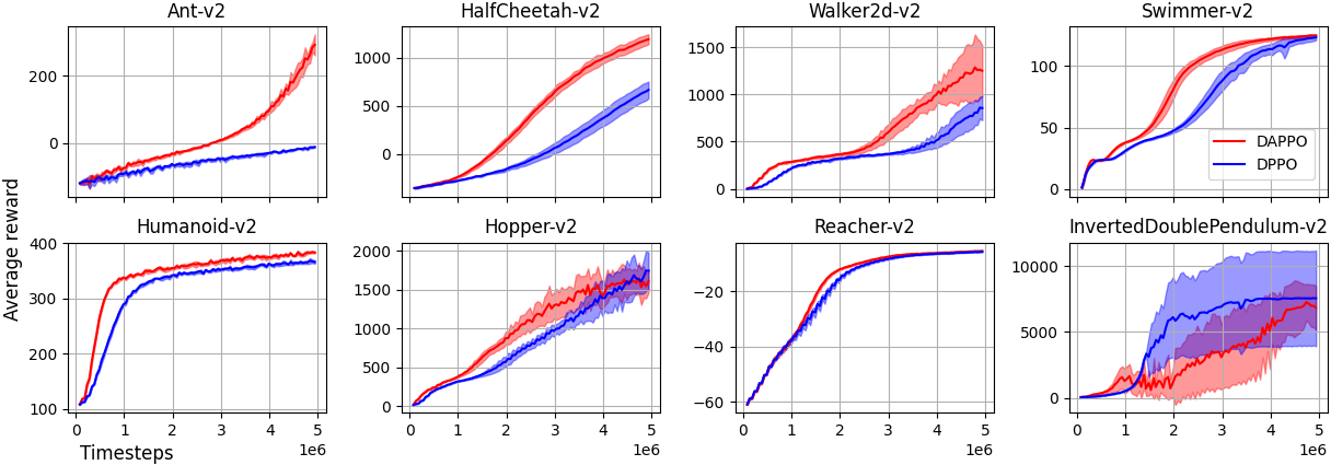
Figure 1: Training curves: DAPPO vs DPPO. Plots show average reward and std over 5 seeds. x-axis is number of timesteps up to 5M.

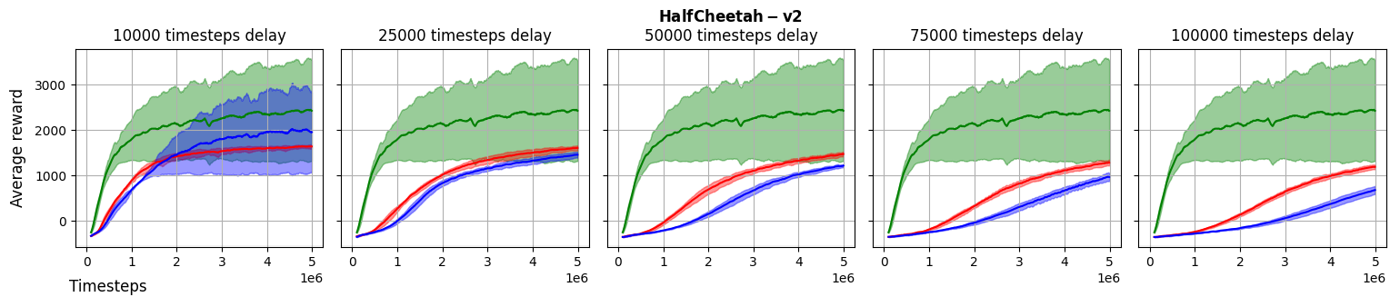
Figure 2: Training curves with different fixed delay length: DAPPO vs DPPO with different delay, alongside PPO without delays. Plots show average reward and std over 5 seeds. x-axis is number of timesteps up to 5M.

We start in a similar way to $\textsc{Bias}_{1}$, and bound $\textsc{Bias}_{2}$ by:

$$H\sqrt{\gamma n}\sum_{k,h}\mathbb{E}_{s,a\sim q^{*}_{h}}\big{[}r_{h}^{k}(s,a)\|\phi_{h}(s,a)\|_{\hat{\Sigma}_{h}^{k,+}}\big{]}$$ (14)

$$+H\sqrt{n}\sum_{k,h}\mathbb{E}_{s,a\sim q^{*}_{h}}\big{[}(1-r_{h}^{k}(s,a))\big{]}.$$ (15)

We handle Eq. 14 like Eq. 12, so for $\beta_{2}=H\sqrt{\gamma n}$ we get that $\eqref{eq:linear Q main bias2 bonus}+\textsc{Bonus}_{2}\lesssim\sqrt{\gamma}H^{2}nK$. Term (15) on the other hand might be of order of $K$ due to mismatch between $\pi^{*}_{h}(a|s)$ in the expectation and $\max\{\pi_{h}^{k+d^{k}}(a|s),\pi_{h}^{k}(a|s)\}$ in the denominator of $r_{h}^{k}(s,a)$. To address that, we design the novel bonus term $b_{h}^{k,r}(s,a)$. Summing Eq. 15 with $\textsc{Bonus}_{r}$ essentially allows us to substitute $\pi^{*}_{h}(a|s)$ by $\pi^{k}_{h}(a|s)$, which gives: $\eqref{eq:linear Q main bias2 bonus}+\textsc{Bonus}_{r}\lesssim\sum_{k,h}\mathbb{E}_{s\sim q_{h}^{*}}\|\pi_{h}^{k+d^{k}}(\cdot|s)-\pi_{h}^{k}(\cdot|s)\|_{1}\lesssim\frac{\eta}{\gamma}H^{3}\sqrt{n}(K+D)$.

Finally, Drift is also bounded by the $\ell_{1}$-distance above and further by $\frac{\eta}{\gamma}H^{4}(K+D)$. Summing the regret from all terms and optimizing over $\eta$ and $\gamma$ completes the proof. ∎

5 Delay-Adapted PPO and Experiments

In this section we show how our generic delay adaptation method extends to state-of-the-art deep RL methods, and demonstrate its great potential through simple experiments on popular MuJoCo environments (Todorov et al., 2012). We note that here we follow the standard convention that use rewards in deep RL rather than costs as in the rest of the paper. Due to lack of space, here we only provide an overview of the method and main experiment. For additional experiments and full implementation details see Appendix F.

The highly successful TRPO algorithm Schulman et al. (2015) is a deep RL policy-gradient method that builds on the same PO principles discussed in this paper. Specifically, it follows the Policy Iteration paradigm with a “soft” policy improvement step, where the policy is now approximated by a Deep Neural Network with parameters $\theta$. While our update step (Eq. 1) is equivalent to maximizing an objective with a KL-regularization term (Shani et al., 2020a), TRPO replaces it by a constraint which results in maximizing the objective $L^{k}_{TRPO}(\theta)=\sum_{h=1}^{H}\frac{\pi^{\theta}(a_{h}|s_{h})}{\pi^{\theta^{k}}(a_{h}|s_{h})}\hat{A}_{h}$ subject to a constraint that keeps the new and the old policies close in terms of KL-divergence. Here, $\hat{A}_{h}$ is an estimate of the advantage function which replaces the $Q$-function in our formulation to further reduce variance (Sutton et al., 1999).

While successful, TRPO’s constrained optimization is computationally expensive. Thus, PPO (Schulman et al., 2017) removes the explicit constraint and replaces it with a sophisticated clipping technique that allows to keep strong empirical performance while only optimizing the following (non-constrained) objective:

$$L^{k}(\theta)=\sum_{h=1}^{H}\min\left\{g^{k}_{h}(\theta)\hat{A}_{h},\text{clip}_{1\pm\epsilon}\left(g^{k}_{h}(\theta)\right)\hat{A}_{h}\right\},$$ (16)

where $g^{k}_{h}(\theta)=\frac{\pi^{\theta}(a_{h}|s_{h})}{\pi^{\theta^{k}}(a_{h}|s_{h})}$ and $\text{clip}_{1\pm\epsilon}(x)$ clips $x$ between $1-\epsilon$ and $1+\epsilon$. This objective essentially zeros the gradient whenever the policy changes too much, and thus replaces the need for an explicit constraint (see more details in Schulman et al. (2017)). Next, we adapt PPO to delayed feedback.

With delayed feedback, the trajectory that arrives at time $k$ was generated using policy $\pi^{\theta^{k-d}}$. Thus, a naive adaptation would be to optimize Eq. 16 but replacing $\pi^{\theta^{k}}$ with $\pi^{\theta^{k-d}}$. We will refer to this algorithm as Delayed PPO (DPPO). As this paper shows, DPPO is likely to suffer from large variance which can be reduced when multiplying the objective by the delay-adapted ratio $r^{k}_{h}(s,a)$. The result is our novel Delay-Adapted PPO (DAPPO) which optimizes:

$$L^{k}_{DA}(\theta)=\sum_{h=1}^{H}\min\left\{R^{k}_{h}(\theta)\hat{A}_{h},\text{clip}_{1\pm\epsilon}\left(R^{k}_{h}(\theta)\right)\hat{A}_{h}\right\},$$

for $R^{k}_{h}(\theta)=\frac{\pi^{\theta}(a_{h}|s_{h})}{\max\{\pi^{\theta^{k-d}}(a_{h}|s_{h}),\pi^{\theta^{k}}(a_{h}|s_{h})\}}$. Another alternative, which we call Non-Delayed PPO (NDPPO), is to run the original PPO and ignore the fact that feedback is delayed. This results in a highly unstable algorithm which is likely to suffer from large bias due to the mismatch between the policy $\pi^{\theta^{k-d}}$ that generated the trajectory and the policy $\pi^{\theta^{k}}$ which is used to re-weight the estimator.

Fig. 1 compares the performance of DPPO and DAPPO over $8$ MuJoCo environments. We use a fixed delay of $10^{5}$ timesteps while the total number of timestamps is $5\cdot 10^{6}$. Results are averaged over 5 runs and the shaded areas around the curves indicate standard deviation. Note that the only difference between the algorithms is the objective, we did not tune hyper-parameters or modify network architecture. DAPPO outperforms DPPO in at least $4$ environments and is on par with DPPO in the rest. The only exception is InvertedDoublePendulum, but it is important to note that this environment is extremely noisy.

Fig. 2 compares the training curves of DPPO vs DAPPO in the Swimmer environment (for more environments see Section F.3) with different delays in $\{10000,25000,50000,75000,100000\}$, alongside the training curve of PPO without delay. As expected, when the delay is relatively small (e.g., $10000$), there is no significant difference between learning with or without delayed feedback. As the delay becomes larger, the performance of all algorithms drops (but at different rates).

These empirical results support our claim that handling delays via the delay-adapted ratio extends naturally beyond the tabular and Linear-$Q$ settings to practical deep function approximation. Surprisingly, even in this simple case, delays cause significant drop in performance which demonstrates the great importance of delay-adapted algorithms. Our novel method makes a significant step towards practical deep RL algorithms that are robust to delayed feedback. Finally, we note that NDPPO is omitted from the graphs because it does not converge (as expected). Instead, it oscillates between high and low reward (see Appendix F for more details).

6 Future Work

We leave a few open questions for future work. In the tabular case, it still remains unclear what is the optimal dependency under delayed feedback in terms of the horizon $H$. Another future direction is to further improve our results in the Linear Function Approximation setting and extend them to the case where a simulator is unavailable. This is in particular important in light of very recent advancement in the non-delayed setting Sherman et al. (2023); Dai et al. (2023) which significantly improve Luo et al. (2021). Finally, our experiment demonstrate the potential that delay-adaptation methods have for deep RL applications. However, a much more thorough empirical study needs to be done in order to fully understand the implications of these methods on deep RL.

Appendix

Appendix A Related Work

In this section we provide a full review of the literature related to regret minimization in adversarial MDP with delayed feedback. For completeness, we include topics that are not directly related to this paper.

Delays in RL without Regret Analysis.

Delays were studied in the practical RL literature (Schuitema et al., 2010; Liu et al., 2014; Changuel et al., 2012; Mahmood et al., 2018; Derman et al., 2021), but this is not related the topic of this paper. In the theory literature, most previous work (Katsikopoulos & Engelbrecht, 2003; Walsh et al., 2009) considered delays in the observation of the state. That is, when the agent takes an action she is not certain what is the current state, and will only observe it in delay. This setting is much more related to partially observable MDPs (POMDPs) and motivated by scenarios like robotics system delays. Unfortunately, even planning is computationally hard (exponential in the delay $d$) for delayed state observability (Walsh et al., 2009). The topic studied in this paper (i.e., delayed feedback) is inherently different, and is motivated by settings like recommendation systems. Importantly, unlike delayed state observability, it is not computationally hard to handle delayed feedback. The challenges of delayed feedback are very different than the ones of delayed state observability, and include policy updates that occur in delay and exploration without observing feedback (Lancewicki et al., 2022b).

Delays in RL with Regret Analysis.

This line of work is related to this paper the most. Howson et al. (2021) studied delayed feedback in stochastic MDPs, and assume that the delays are also stochastic, i.e., sampled i.i.d from a fixed (unknown) distribution. This is a restrictive assumption since it does not allow dependencies between costs and delays that are very common in practice. In adversarial MDPs, delayed feedback was first studied by Lancewicki et al. (2022b). They proposed Policy Optimization algorithms that handle delays, but focused on the case of full-information feedback where the agent observes the entire cost function in the end of the episode instead of bandit feedback (where the agent observes only costs along its trajectory). Full-information feedback is not a realistic assumption in most applications, and for bandit feedback they only prove sub-optimal regret of $(K+D)^{2/3}$ (ignoring dependencies in $S,A,H$). Later, Jin et al. (2022) managed to achive a near-optimal regret bound of $\tilde{\mathcal{O}}(H\sqrt{SAK}+(HSA)^{1/4}H\sqrt{D})$ for the case of known transition function and $\tilde{\mathcal{O}}(H^{2}S\sqrt{AK}+(HSA)^{1/4}H\sqrt{D})$ for the case of unknown transitions. However, their algorithm is based on the O-REPS method (Zimin & Neu, 2013) which requires solving a computationally expensive global optimization problem and cannot be extended to function approximation. Recently, Dai et al. (2022) showed that delayed feedback in adversarial MDPs can also be dealt with using Follow-The-Perturbed-Leader (FTPL) algorithms. The efficiency of FTPL algorithms is similar to Policy Optimization, but their regret bound is only $\tilde{\mathcal{O}}(H^{2}S\sqrt{AK}+\sqrt{HSA}\cdot H\sqrt{D})$.

Delays in multi-arm bandit (MAB).

Delays were extensively studied in MAB and online optimization both in the stochastic setting (Dudik et al., 2011; Agarwal & Duchi, 2012; Vernade et al., 2017; 2020; Pike-Burke et al., 2018; Cesa-Bianchi et al., 2018; Zhou et al., 2019; Gael et al., 2020; Lancewicki et al., 2021; Cohen et al., 2021a; Howson et al., 2022), and the adversarial setting (Quanrud & Khashabi, 2015; Cesa-Bianchi et al., 2016; Thune et al., 2019; Bistritz et al., 2019; Zimmert & Seldin, 2020; Ito et al., 2020; Gyorgy & Joulani, 2021; Van Der Hoeven & Cesa-Bianchi, 2022; Masoudian et al., 2022). However, as discussed in Lancewicki et al. (2022b), delays introduce new challenges in MDPs that do not appear in MAB.

Regret minimization in Tabular RL.

There exists a rich literature on regret minimization in tabular MDPs. In the stochastic case, the algorithms are mainly built on the optimism in face of uncertainty approach (Jaksch et al., 2010; Azar et al., 2017; Dann et al., 2017; Jin et al., 2018; Efroni et al., 2019; Tarbouriech et al., 2020; 2021; Rosenberg & Mansour, 2021a; Rosenberg et al., 2020; Cohen et al., 2021b; Chen et al., 2021). In the adversarial case, while a few algorithms use FTPL (Neu et al., 2012; Dai et al., 2022), most algorithms are based on either the O-REPS method (Zimin & Neu, 2013; Rosenberg & Mansour, 2019b; a; 2021b; Jin et al., 2020a; 2021; Jin & Luo, 2020; Lancewicki et al., 2022a; Chen et al., 2020b; Chen & Luo, 2021) or on Policy Optimization (Even-Dar et al., 2009; Neu et al., 2010a; b; 2014; Shani et al., 2020b; Luo et al., 2021; Chen et al., 2022b). Note that regret minimization in standard episodic MDPs is a special case of the model considered in this paper where $d^{k}=0$ for every episode $k$.

Regret minimization in RL with Linear Function Approximation.

In recent years the literature on regret minimization in RL has expanded to linear function approximation. While in the stochastic case algorithms are still based on optimism (Jin et al., 2020b; Yang & Wang, 2019; Zanette et al., 2020a; b; Ayoub et al., 2020; Zhou et al., 2021; Zhou & Gu, 2022; Vial et al., 2022; Chen et al., 2022a; Min et al., 2022), in the adversarial case O-REPS cannot be extended to linear function approximation without additional assumptions so algorithms are mostly based on Policy Optimization (Cai et al., 2020; Abbasi-Yadkori et al., 2019; Agarwal et al., 2020; He et al., 2022; Neu & Olkhovskaya, 2021; Luo et al., 2021; Wei et al., 2021).

Policy Optimization in Deep RL.

Policy Optimization is among the most widely used methods in deep Reinforcement Learning (Lillicrap et al., 2015; Levine et al., 2016; Gu et al., 2017). The origins of these algorithms are Policy Gradient Sutton & Barto (2018), Conservative Policy Iteration (Kakade & Langford, 2002) and Natural Policy Gradient (Kakade, 2001). These have evolved into some of the state-of-the-art algorithms in RL, e.g., Trust Region Policy Optimization (TRPO) (Schulman et al., 2015), Proximal Policy Optimization (PPO) (Schulman et al., 2017) and Soft Actor-Critic (SAC) (Haarnoja et al., 2018). Recently, the connections between deep RL policy optimization algorithms and online learning regularization methods (like Follow-The-Regularized-Leader and Online-Mirror-Descent) were studied and explained (Shani et al., 2020a; Tomar et al., 2022).

Remark A.1 (The Loop-Free Assumption).

We warn the readers that some of the works mentioned in this section (mainly in the adversarial MDP literature, e.g., Luo et al. (2021)) present a slightly different dependence in the horizon $H$. The reason is that they make the loop-free assumption, i.e., they assume that the state space consists of $H$ disjoint sets $\mathcal{S}=\mathcal{S}_{1}\cup\mathcal{S}_{2}\cup\dots\cup\mathcal{S}_{H}$ such that in step $h$ the agent can only be found in states from the set $\mathcal{S}_{h}$. Effectively, this means that their state space is larger than ours by a factor of $H$. So when they present a regret bound of $\tilde{\mathcal{O}}(H^{2}S\sqrt{AK})$, this implies a bound of $\tilde{\mathcal{O}}(H^{3}S\sqrt{AK})$ in the model presented in this paper. We emphasize that these differences are only due to different models, and not due to actual different regret bounds.

Appendix B Delay-Adapted Policy Optimization for (Tabular) Adversarial MDP with Known Transition

Algorithm 3 Delay-Adapted Policy Optimization with Known Transition Function (Tabular)

  Input: state space $\mathcal{S}$, action space $\mathcal{A}$, horizon $H$, transition function $p$, learning rate $\eta>0$, exploration parameter $\gamma>0$.

  Initialization: Set $\pi_{h}^{1}(a\mid s)=\nicefrac{{1}}{{A}}$ for every $(s,a,h)\in\mathcal{S}\times\mathcal{A}\times[H]$.

  for $k=1,2,\dots,K$ do

     Play episode $k$ with policy $\pi^{k}$, observe trajectory $\{(s^{k}_{h},a^{k}_{h})\}_{h=1}^{H}$ and compute $q^{k}_{h}(s)$ for every $(s,h)\in\mathcal{S}\times[H]$.

      # Policy Evaluation

     for $j$ such that $j+d^{j}=k$ do

        Observe bandit feedback $\{c^{j}_{h}(s^{j}_{h},a^{j}_{h})\}_{h=1}^{H}$ and set $B^{j}_{H+1}(s,a)=0$ for every $(s,a)\in\mathcal{S}\times\mathcal{A}$.

        for $h=H,H-1,\dots,1$ do

           for $(s,a)\in\mathcal{S}\times\mathcal{A}$ do

              Compute $r^{j}_{h}(s,a)=\frac{\pi^{j}_{h}(a\mid s)}{\max\{\pi^{j}_{h}(a\mid s),\pi_{h}^{k}(a\mid s)\}}$ and $L^{j}_{h}=\sum_{h^{\prime}=h}^{H}c^{j}_{h^{\prime}}(s^{j}_{h^{\prime}},a^{j}_{h^{\prime}})$.

              Compute $\hat{Q}_{h}^{j}(s,a)=r^{j}_{h}(s,a)\frac{\mathbb{I}\{s_{h}^{j}=s,a_{h}^{j}=a\}L^{j}_{h}}{q_{h}^{j}(s)\pi_{h}^{j}(a\mid s)+\gamma}$ and $b^{j}_{h}(s)=\sum_{a\in\mathcal{A}}\frac{3\gamma H\pi^{k}_{h}(a\mid s)r^{j}_{h}(s,a)}{q^{j}_{h}(s)\pi^{j}_{h}(a\mid s)+\gamma}$.

              Compute $B_{h}^{j}(s,a)=b_{h}^{j}(s)+\sum_{s^{\prime}\in\mathcal{S},a^{\prime}\in\mathcal{A}}p_{h}(s^{\prime}\mid s,a)\pi_{h+1}^{j}(a^{\prime}\mid s^{\prime})B^{j}_{h+1}(s^{\prime},a^{\prime})$.

           end for

        end for

     end for

      # Policy Improvement

     Define the policy $\pi^{k+1}$ for every $(s,a,h)\in\mathcal{S}\times\mathcal{A}\times[H]$ by:

$$\pi^{k+1}_{h}(a\mid s)=\frac{\pi^{k}_{h}(a\mid s)\exp\left(-\eta\sum_{j:j+d^{j}=k}(\hat{Q}_{h}^{j}(s,a)-B_{h}^{j}(s,a))\right)}{\sum_{a^{\prime}\in\mathcal{A}}\pi^{k}_{h}(a^{\prime}\mid s)\exp\left(-\eta\sum_{j:j+d^{j}=k}(\hat{Q}_{h}^{j}(s,a^{\prime})-B_{h}^{j}(s,a^{\prime}))\right)}.$$

  end for

Theorem B.1.

Set $\eta=\left(H^{2}SAK+H^{4}(K+D)\right)^{-1/2}$ and $\gamma=2\eta H$. Running Algorithm 3 in an adversarial MDP $\mathcal{M}=(\mathcal{S},\mathcal{A},H,p,\{c^{k}\}_{k=1}^{K})$ with known transition function and delays $\{d^{k}\}_{k=1}^{K}$ guarantees, with probability at least $1-\delta$,

$$R_{K}=\mathcal{O}\left(H^{2}\sqrt{SAK}\log\frac{KHSA}{\delta}+H^{3}\sqrt{K+D}\log\frac{KHSA}{\delta}+H^{4}d_{max}\log\frac{KHSA}{\delta}\right).$$

B.1 The good event

Let $\iota=10\log\frac{10KHSA}{\delta}$, $\tilde{\mathcal{H}}^{k}$ be the history of episodes $\{j:j+d^{j}<k\}$, and define $\mathbb{E}_{k}[\cdot]=\mathbb{E}\big{[}\cdot\mid\tilde{\mathcal{H}}^{k+d^{k}}\big{]}$ Define the following events:

$$E^{d} =\left\{\forall(h,s).\ \sum_{k=1}^{K}\sum_{j=1}^{K}\sum_{a}\mathbb{I}\{j\leq k+d^{k}<j+d^{j}\}\pi_{h}^{k+d^{k}}(a\mid s)(\hat{Q}_{h}^{k}(s,a)-Q_{h}^{k}(s,a))\leq\frac{10H^{2}d_{max}\log\frac{10HS}{\delta}}{\gamma}\right\}$$

$$E^{*} =\left\{\sum_{k=1}^{K}\sum_{h,s,a}q^{*}_{h}(s,a)(\hat{Q}_{h}^{k}(s,a)-Q_{h}^{k}(s,a))\leq\frac{H^{2}\log\frac{10HSA}{\delta}}{\gamma}\right\}$$

$$E^{b} =\left\{\sum_{k=1}^{K}\sum_{h,s,a}\frac{q_{h}^{*}(s)\pi_{h}^{k+d^{k}}(a\mid s)r^{k}_{h}(s,a)\mathbb{I}\{s_{h}^{k}=s,a_{h}^{k}=a\}}{(q_{h}^{k}(s,a)+\gamma)^{2}}-\sum_{k=1}^{K}\sum_{h,s,a}\frac{q_{h}^{*}(s)\pi_{h}^{k+d^{k}}(a\mid s)r^{k}_{h}(s,a)}{q_{h}^{k}(s,a)+\gamma}\leq\frac{H}{\gamma^{2}}\ln\frac{10H}{\delta}\right\}$$

$$E^{f} =\bBigg@{3}\{\sum_{k=1}^{K}\mathbb{E}_{k}\left[\sum_{h,s}q_{h}^{*}(s)\left\langle\pi_{h}^{k+d^{k}}(\cdot\mid s),\hat{Q}_{h}^{k}(s,\cdot)\right\rangle\right]-\sum_{k=1}^{K}\sum_{h,s}q_{h}^{*}(s)\left\langle\pi_{h}^{k+d^{k}}(\cdot\mid s),\hat{Q}_{h}^{k}(s,\cdot)$$

$$\qquad\qquad\qquad\qquad\qquad\qquad\qquad\qquad\qquad\qquad\qquad\qquad\qquad\qquad\qquad\leq\frac{1}{3}\sum_{k=1}^{K}\sum_{h,s}q_{h}^{*}(s)b_{h}^{k}(s)+\frac{H^{2}}{\gamma}\ln\frac{10}{\delta}\bBigg@{3}\}$$

The good event is the intersection of the above events. The following lemma establishes that the good event holds with high probability.

Lemma B.2 (The Good Event).

Let $\mathbb{G}=E^{d}\cap E^{*}\cap E^{b}\cap E^{f}$ be the good event. It holds that $\Pr[\mathbb{G}]\geq 1-\delta$.

Proof.

We’ll show that each of the events $\lnot E^{d},\lnot E^{*},\lnot E^{b},\lnot E^{f}$ holds with probability of at most $\delta/4$ and so by the union bound $\Pr[\mathbb{G}]\geq 1-\delta$.

Event $E^{d}$: Fix $s$ and $h$. For every $(h^{\prime},s^{\prime},a$) set:

$$z_{h^{\prime}}^{k}(s^{\prime},a) =\mathbb{I}\left\{s^{\prime}=s,h^{\prime}=h\right\}\sum_{j=1}^{K}\mathbb{I}\{j\leq k+d^{k}<j+d^{j}\}\pi_{h}^{k+d^{k}}(a\mid s)r^{k}_{h}(s,a)Q_{h}^{j}(s,a)$$

$$Z_{h^{\prime}}^{k}(s^{\prime},a) =\mathbb{I}\left\{s^{\prime}=s,h^{\prime}=h\right\}\sum_{j=1}^{K}\mathbb{I}\{j\leq k+d^{k}<j+d^{j}\}\pi_{h}^{k+d^{k}}(a\mid s)r^{k}_{h}(s,a)M_{h}^{k}(s,a)$$

$$M_{h}^{k}(s,a) =\mathbb{I}\{s_{h}^{k}=s,a_{h}^{k}=a\}\sum_{\tilde{h}=1}^{H}c_{\tilde{h}}^{k}(s_{\tilde{h}}^{k},a_{\tilde{h}}^{k})+(1-\mathbb{I}\{s_{h}^{k}=s,a_{h}^{k}=a\})Q_{h}^{k}(s,a).$$

Note that $\mathbb{E}_{k}[Z_{h^{\prime}}^{k}(s^{\prime},a)]=z_{h^{\prime}}^{k}(s^{\prime},a)$ and,

$$\sum_{h^{\prime},s^{\prime},a}\frac{\mathbb{I}\{s_{h}^{k}=s,a_{h}^{k}=s\}Z_{h}^{k}(s,a)}{q_{h}^{k}(s,a)+\gamma} =\sum_{j=1}^{K}\sum_{a}\mathbb{I}\{j\leq k+d^{k}<j+d^{j}\}\pi_{h}^{k+d^{k}}(a\mid s)\hat{Q}_{h}^{k}(s,a)$$

$$\sum_{h^{\prime},s^{\prime},a}z_{h}^{k}(s,a) \leq\sum_{j=1}^{K}\sum_{a}\mathbb{I}\{j\leq k+d^{k}<j+d^{j}\}\pi_{h}^{k+d^{k}}(a\mid s)Q_{h}^{k}(s,a),$$

where in the inequality we used the fact that $r^{k}_{h}(s,a)\leq 1$. Finally, we use Lemma E.5 with $\tilde{q}_{h}^{k}(s,a)=q_{h}^{k}(s,a)$ and $R\leq 2Hd_{max}$ since the number of $j$s such that $j\leq k+d^{k}<j+d^{j}$ is at most $2d_{max}$. Thus, the event holds for $(s,h)$ with probability $1-\frac{\delta}{10HS}$. By taking the union bound over all $h$ and $s$, $E^{d}$ holds with probability $1-\frac{\delta}{10}$.

Event $E^{*}$ (Lemma C.2 of Luo et al. (2021)): $E^{*}$ holds with probability of at least $1-\delta/10$ by applying Lemma E.5 with $\tilde{q}_{h^{\prime}}^{k}(s^{\prime},a)=q_{h^{\prime}}^{k}(s^{\prime}a)$, $z_{h}^{k}(s,a)=q^{*}_{h}(s,a)r^{k}_{h}(s,a)Q_{h}^{k}(s,a)$ and,

$$Z_{h}^{k}(s,a)=q_{h}^{*}(s,a)r^{k}_{h}(s,a)\left(\mathbb{I}\{s_{h}^{k}=s,a_{h}^{k}=a\}\sum_{h^{\prime}=1}^{H}c_{h^{\prime}}^{k}(s_{h^{\prime}}^{k},a_{h^{\prime}}^{k})+(1-\mathbb{I}\{s_{h}^{k}=s,a_{h}^{k}=a\})Q_{h}^{k}(s,a)\right).$$

Note that $R\leq H$, $\frac{\mathbb{I}\{s_{h}^{k}=s,a_{h}^{k}=s\}Z_{h}^{k}(s,a)}{\tilde{q}_{h}^{k}(s,a)+\gamma}=q^{*}_{h}(s,a)\hat{Q}_{h}^{k}(s,a)$ and $\frac{q_{h}^{k}(s,a)z_{h}^{k}(s,a)}{\tilde{q}_{h}^{k}(s,a)}\leq q^{*}_{h}(s,a)Q_{h}^{k}(s,a)$.

Event $E^{b}$: Similar to the last two events, $E^{b}$ holds with probability of at least $1-\delta/10$ by applying Lemma E.5 with $\tilde{q}_{h^{\prime}}^{k}(s^{\prime},a)=q_{h^{\prime}}^{k}(s^{\prime},a)$ and $z_{h}^{k}(s,a)=Z_{h}^{k}(s,a)=\frac{q_{h}^{*}(s)\pi_{h}^{k+d^{k}}(a\mid s)r^{k}_{h}(s,a)}{q_{h}^{k}(s,a)+\gamma}$.

Event $E^{f}$: Let $Y_{k}=\sum_{h,s}q_{h}^{*}(s)\left\langle\pi_{h}^{k+d^{k}}(\cdot\mid s),\hat{Q}_{h}^{k}(s,\cdot)\right\rangle$. We’ll use a variant of Freedman’s inequality (Lemma E.3) to bound $\sum_{k=1}^{K}\mathbb{E}_{k}[Y_{k}]-\sum_{k=1}^{K}Y_{k}$. Note that:

$$\mathbb{E}_{k}\left[Y_{k}^{2}\right] =\mathbb{E}_{k}\left[\left(\sum_{h,s,a}q_{h}^{*}(s)\pi_{h}^{k+d^{k}}(a\mid s)\hat{Q}_{h}^{k}(s,a)\right)^{2}\right]$$

$$\leq\mathbb{E}_{k}\left[\left(\sum_{h,s,a}q_{h}^{*}(s)\pi_{h}^{k+d^{k}}(a\mid s)\right)\left(\sum_{h,s,a}q_{h}^{*}(s)\pi_{h}^{k+d^{k}}(a\mid s)(\hat{Q}_{h}^{k}(s,a))^{2}\right)\right]$$

$$\leq H\mathbb{E}_{k}\left[\sum_{h,s,a}q_{h}^{*}(s)\pi_{h}^{k+d^{k}}(a\mid s)\frac{r^{k}_{h}(s,a)^{2}(L_{h}^{k})^{2}\mathbb{I}\{s_{h}^{k}=s,a_{h}^{k}=a\}}{(q_{h}^{k}(s,a)+\gamma)^{2}}\right]$$

$$\leq H^{3}\sum_{h,s,a}q_{h}^{*}(s)\pi_{h}^{k+d^{k}}(a\mid s)\frac{q^{k}_{h}(s,a)r^{k}_{h}(s,a)}{(q_{h}^{k}(s,a)+\gamma)^{2}}$$

$$\leq H^{3}\sum_{h,s,a}\frac{q_{h}^{*}(s)\pi_{h}^{k+d^{k}}(a\mid s)r^{k}_{h}(s,a)}{q_{h}^{k}(s,a)+\gamma},$$

where the first inequality is Cauchy-Schwartz inequality. Also, $|Y_{k}|\leq\frac{H^{2}}{\gamma}$. Therefore by Lemma E.3 with probability $1-\delta/10$,

$$\sum_{k=1}^{K}\mathbb{E}_{k}[Y_{k}]-\sum_{k=1}^{K}Y_{k} \leq\gamma H\sum_{k=1}^{K}\left(\sum_{h,s,a}\frac{q_{h}^{*}(s)\pi_{h}^{k+d^{k}}(a\mid s)r^{k}_{h}(s,a)}{q_{h}^{k}(s,a)+\gamma}\right)+\frac{H^{2}}{\gamma}\ln\frac{10}{\delta}$$

$$=\frac{1}{3}\sum_{k=1}^{K}\sum_{h,s}q_{h}^{*}(s)b_{h}^{k}(s)+\frac{H^{2}}{\gamma}\ln\frac{10}{\delta}.\qed$$

B.2 Proof of the main theorem

Proof of Theorem B.1.

By Lemma B.2, the good event holds with probability $1-\delta$. We now analyze the regret under the assumption that the good event holds. We start with the following regret decomposition,

$$R_{K}= \sum_{k=1}^{K}\sum_{h,s}q_{h}^{*}(s)\left\langle\pi_{h}^{k}(\cdot\mid s)-\pi_{h}^{*}(\cdot\mid s),Q_{h}^{k}(s,\cdot)\right\rangle=\underbrace{\sum_{k=1}^{K}\sum_{h,s}q_{h}^{*}(s)\left\langle\pi_{h}^{k+d^{k}}(\cdot\mid s),Q_{h}^{k}(s,\cdot)-\hat{Q}_{h}^{k}(s,\cdot)\right\rangle}_{\textsc{Bias}_{1}}$$

$$+\underbrace{\sum_{k=1}^{K}\sum_{h,s}q_{h}^{*}(s)\left\langle\pi_{h}^{*}(\cdot\mid s),\hat{Q}_{h}^{k}(s,\cdot)-Q_{h}^{k}(s,\cdot)\right\rangle}_{\textsc{Bias}_{2}}+\underbrace{\sum_{k=1}^{K}\sum_{h,s}q_{h}^{*}(s)\left\langle\pi_{h}^{k}(\cdot\mid s)-\pi_{h}^{*}(\cdot\mid s),B_{h}^{k}(s,\cdot)\right\rangle}_{\textsc{Bonus}}$$

$$+\underbrace{\sum_{k=1}^{K}\sum_{h,s}q_{h}^{*}(s)\left\langle\pi_{h}^{k+d^{k}}(\cdot\mid s)-\pi_{h}^{*}(\cdot\mid s),\hat{Q}_{h}^{k}(s,\cdot)-B_{h}^{k}(s,\cdot)\right\rangle}_{\textsc{Reg}}$$

$$+\underbrace{\sum_{k=1}^{K}\sum_{h,s}q_{h}^{*}(s)\left\langle\pi_{h}^{k}(\cdot\mid s)-\pi_{h}^{k+d^{k}}(\cdot\mid s),Q_{h}^{k}(s,\cdot)-B_{h}^{k}(s,\cdot)\right\rangle}_{\textsc{Drift}},$$

where the first equality is by Lemma E.1 (value difference lemma). $\textsc{Bias}_{2}$ is bounded under event $E^{*}$ by $\mathcal{O}\left(\frac{H^{2}\iota}{\gamma}\right)$. The other four terms are bounded in Lemmas B.3, B.4, B.6 and B.7. Overall,

$$R_{K} \leq\underbrace{\frac{2}{3}\sum_{k=1}^{K}\sum_{h,s}q_{h}^{*}(s)b_{h}^{k}(s)+\mathcal{O}\left(\eta H^{4}(K+D)+\frac{\eta H^{4}d_{max}\iota}{\gamma}+\frac{H^{2}}{\gamma}\iota\right)}_{\textsc{Bais}_{1}}+\underbrace{\mathcal{O}\left(\frac{H^{2}}{\gamma}\iota\right)}_{\textsc{Bais}_{2}}$$

$$\qquad+\underbrace{3\gamma H^{2}SAK-\sum_{k=1}^{K}\sum_{h,s}q_{h}^{*}(s)b_{h}^{k}(s)}_{\textsc{Bonus}}+\underbrace{\frac{H\ln A}{\eta}+\frac{1}{3}\sum_{k=1}^{K}\sum_{h,s}q_{h}^{*}(s)b_{h}^{k}(s)+\mathcal{O}\left(\eta H^{5}K+\eta\frac{H^{3}\iota}{\gamma^{2}}\right)}_{\textsc{Reg}}$$

$$\qquad+\underbrace{\mathcal{O}\left(\eta H^{5}(K+D)+\frac{\eta H^{5}d_{max}\iota}{\gamma}\right)}_{\textsc{Drift}}$$

$$\leq\mathcal{O}\left(\frac{H\ln A}{\eta}+\gamma H^{2}SAK+\eta H^{5}(K+D)+\eta\frac{H^{3}\iota}{\gamma^{2}}+\frac{H^{2}}{\gamma}\iota+\frac{\eta H^{5}d_{max}\iota}{\gamma}\right).$$

For $\eta=\frac{1}{\sqrt{H^{2}SAK+H^{4}(K+D)}}$ and $\gamma=2\eta H$, we get: $R_{K}\leq\mathcal{O}\left(H^{2}\sqrt{SAK}\iota+H^{3}\sqrt{D}\iota+H^{3}\sqrt{K}\iota+H^{4}d_{max}\iota\right).$ ∎

B.3 Bound on $\textsc{Bias}_{1}$

Lemma B.3.

Under the good event, $\textsc{Bias}_{1}\leq\frac{2}{3}\sum_{k=1}^{K}\sum_{h,s}q_{h}^{*}(s)b_{h}^{k}(s)+\mathcal{O}\left(\eta H^{4}(K+D)+\frac{\eta H^{4}d_{max}\iota}{\gamma}+\frac{H^{2}}{\gamma}\iota\right).$

Proof.

Let $Y_{k}=\sum_{h,s}q_{h}^{*}(s)\left\langle\pi_{h}^{k+d^{k}}(\cdot\mid s),\hat{Q}_{h}^{k}(s,\cdot)\right\rangle$. It holds that

$$\textsc{Bias}_{1}=\sum_{k=1}^{K}\sum_{h,s}q_{h}^{*}(s)\left\langle\pi_{h}^{k+d^{k}}(\cdot\mid s),Q_{h}^{k}(s,\cdot)\right\rangle-\sum_{k=1}^{K}\mathbb{E}_{k}[Y_{k}]+\sum_{k=1}^{K}\mathbb{E}_{k}[Y_{k}]-\sum_{k=1}^{K}Y_{k}.$$

Under event $E^{f}$ it holds that

$$\sum_{k=1}^{K}\mathbb{E}_{k}[Y_{k}]-\sum_{k=1}^{K}Y_{k} \leq\frac{1}{3}\sum_{k=1}^{K}\sum_{h,s}q_{h}^{*}(s)b_{h}^{k}(s)+\frac{H^{2}}{\gamma}\ln\frac{10}{\delta}.$$

In addition,

$$\sum_{k=1}^{K} \sum_{h,s}q_{h}^{*}(s)\left\langle\pi_{h}^{k+d^{k}}(\cdot\mid s),Q_{h}^{k}(s,\cdot)\right\rangle-\sum_{k=1}^{K}\mathbb{E}_{k}[Y_{k}]=$$

$$=\sum_{k=1}^{K}\sum_{h,s,a}q_{h}^{*}(s)\pi_{h}^{k+d^{k}}(a\mid s)Q_{h}^{k}(s,a)\left(1-\frac{q_{h}^{k}(s,a)r^{k}_{h}(s,a)}{q_{h}^{k}(s,a)+\gamma}\right)$$

$$=\sum_{k=1}^{K}\sum_{h,s,a}q_{h}^{*}(s)\pi_{h}^{k+d^{k}}(a\mid s)Q_{h}^{k}(s,a)\left(1-\frac{(q_{h}^{k}(s,a)+\gamma)r^{k}_{h}(s,a)}{q_{h}^{k}(s,a)+\gamma}\right)+\sum_{k=1}^{K}\sum_{h,s,a}q_{h}^{*}(s)\pi_{h}^{k+d^{k}}(a\mid s)Q_{h}^{k}(s,a)\frac{\gamma r^{k}_{h}(s,a)}{q_{h}^{k}(s,a)+\gamma}$$

$$\leq\sum_{k=1}^{K}\sum_{h,s,a}q_{h}^{*}(s)\pi_{h}^{k+d^{k}}(a\mid s)Q_{h}^{k}(s,a)(1-r^{k}_{h}(s,a))+\sum_{k=1}^{K}\sum_{h,s,a}q_{h}^{*}(s)\frac{\gamma H\pi_{h}^{k+d^{k}}(a\mid s)r^{k}_{h}(s,a)}{q_{h}^{k}(s,a)+\gamma}$$

$$\leq H\sum_{k=1}^{K}\sum_{h,s,a}q_{h}^{*}(s)\left(\max\{\pi_{h}^{k}(a\mid s),\pi_{h}^{k+d^{k}}(a\mid s)\}-\pi_{h}^{k}(a\mid s)\right)+\sum_{k=1}^{K}\sum_{h,s,a}q_{h}^{*}(s)\frac{\gamma H\pi_{h}^{k+d^{k}}(a\mid s)r^{k}_{h}(s,a)}{q_{h}^{k}(s,a)+\gamma}$$

$$\leq H\sum_{k=1}^{K}\sum_{h,s}q_{h}^{*}(s)\|\pi_{h}^{k+d^{k}}(\cdot\mid s)-\pi_{h}^{k}(\cdot\mid s)\|_{1}+\frac{1}{3}\sum_{k=1}^{K}\sum_{h,s}q_{h}^{*}(s)b_{h}^{k}(s).$$

Finally, using Lemma B.8,

$$\textsc{Bias}_{1} \leq\frac{2}{3}\sum_{k=1}^{K}\sum_{h,s}q_{h}^{*}(s)b_{h}^{k}(s)+H\sum_{h,s}q_{h}^{*}(s)\sum_{k=1}^{K}\|\pi_{h}^{k+d^{k}}(\cdot\mid s)-\pi_{h}^{k}(\cdot\mid s)\|_{1}+\frac{H^{2}}{\gamma}\iota$$

$$\leq\frac{2}{3}\sum_{k=1}^{K}\sum_{h,s}q_{h}^{*}(s)b_{h}^{k}(s)+H\sum_{h,s}q_{h}^{*}(s)\left(\mathcal{O}\left(\eta H^{2}(K+D)+\frac{\eta H^{2}d_{max}\iota}{\gamma}\right)\right)+\frac{H^{2}}{\gamma}\iota$$

$$=\frac{2}{3}\sum_{k=1}^{K}\sum_{h,s}q_{h}^{*}(s)b_{h}^{k}(s)+\mathcal{O}\left(\eta H^{4}(K+D)+\frac{\eta H^{4}d_{max}\iota}{\gamma}\right)+\frac{H^{2}}{\gamma}\iota.\qed$$

B.4 Bound on Bonus

Lemma B.4.

It holds that $\textsc{Bonus}\leq 3\gamma H^{2}SAK-\sum_{k,h,s}q_{h}^{*}(s)b_{h}^{k}(s).$

Proof.

Note that $B_{h}^{k}$ is the $Q$-function of policy $\pi^{k}$ with respect to the cost function $b^{k}$. Hence, by the value difference difference lemma (Lemma E.1),

$$\sum_{h,s}q_{h}^{k}(s)b_{h}^{k}(s)-\sum_{h,s}q_{h}^{*}(s)b_{h}^{k}(s)=V^{\pi^{k}}_{1}(s_{\text{init}};b^{k})-V^{\pi^{*}}(s_{\text{init}};b^{k})=\sum_{h,s}q_{h}^{*}(s)\left\langle\pi_{h}^{k}(\cdot\mid s)-\pi_{h}^{*}(\cdot\mid s),B_{h}^{k}(s,\cdot)\right\rangle.$$

Summing over $k$ we get: $\textsc{Bonus}=\sum_{k,h,s}q_{h}^{k}(s)b_{h}^{k}(s)-\sum_{k,h,s}q_{h}^{*}(s)b_{h}^{k}(s).$ For last,

$$\sum_{k=1}^{K}\sum_{h,s}q_{h}^{k}(s)b^{k}_{h}(s) =3\gamma H\sum_{k=1}^{K}\sum_{h,s,a}\frac{q_{h}^{k}(s)\pi^{k+d^{k}}_{h}(a\mid s)r^{k}_{h}(s,a)}{q_{h}^{k}(s)\pi^{k}_{h}(a\mid s)+\gamma}\leq 3\gamma H^{2}SAK.$$

where the last uses the fact that $\pi^{k+d^{k}}_{h}(a\mid s)r_{h}^{k}(s,a)\leq\pi^{k}_{h}(a\mid s)$. ∎

Remark B.5.

The adaptation to delay via the ratio $r_{h}^{k}(s,a)$ is simple, yet crucial. The main reason is the following. While in MAB the ratio $\pi^{k+d^{k}}_{h}(a\mid s)/\pi^{k}_{h}(a\mid s)$ is always bounded by a constant (Thune et al., 2019, Lemma 11), in MDPs it can be as large as $e^{d_{max}}$. In fact, even the ratio $\pi^{k+1}_{h}(a\mid s)/\pi^{k}_{h}(a\mid s)$ can be of order $e^{d_{max}}$, because even if an action $a$ is chosen with probability close to $1$, the estimator $\hat{Q}_{h}^{k}(s,a)$ can be as large as $\Omega(1/\gamma)$, as long as the visitation probability to state $s$ is smaller than $1/\gamma$. This can cause radical changes in the probability to take action $a$ (and as a consequence in the probability of the rest of the actions in that state). For example, assume we have two actions $a_{1},a_{2}$ with $\pi_{h}^{k}(a_{1}\mid s)=1/(e^{-d_{max}}+1)$, $\pi_{h}^{k}(a_{2}\mid s)=e^{-d_{max}}/(e^{-d_{max}}+1)$ and $q_{h}^{k}(s)\leq\gamma$. Now, assume that the feedback from $d_{max}$ episodes arrive at at the end of episode $k$ for which the agent visited in the state-action pair $(s,a_{1})$. Further assume the cost-to-go from $(s,a_{1})$ was of order $H$. This would imply that $\eta\sum_{j:j+d^{j}=k}(\hat{Q}_{h}^{j}(s,a)-B_{h}^{j}(s,a))\approx d_{max}$. Hence, the probability to take each of the actions under $\pi^{k+1}$ would be approximately $1/2$. In particular, $\pi^{k+1}_{h}(a_{2}\mid s)/\pi^{k}_{h}(a_{2}\mid s)=\Omega((e^{-d_{max}}+1)/e^{-d_{max}})=\Omega(e^{d_{max}})$.

B.5 Bound on Reg

Lemma B.6.

For $\eta\leq\frac{\gamma}{2H}$ it holds that $\textsc{Reg}\leq\frac{H\ln A}{\eta}+\frac{1}{3}\sum_{k,h,s}q_{h}^{*}(s)b_{h}^{k}(s)+\mathcal{O}\left(\eta H^{5}K+\eta\frac{H^{3}\iota}{\gamma^{2}}\right).$

Proof.

By Corollary E.7, since $\max_{k,h,s,a}B_{h}^{k}(s,a)\leq 3H^{2}$,

Reg $$\leq\frac{H\ln A}{\eta}+2\eta\sum_{k,h,s,a}q_{h}^{*}(s)\pi_{h}^{k+d^{k}}(a\mid s)\left(\hat{Q}_{h}^{k}(s,a)-B_{h}^{k}(s,a)\right)^{2}+\mathcal{O}(\eta H^{5}K)$$

$$\leq\frac{H\ln A}{\eta}+2\eta\sum_{k,h,s,a}q_{h}^{*}(s)\pi_{h}^{k+d^{k}}(a\mid s)\hat{Q}_{h}^{k}(s,a)^{2}+2\eta\sum_{k,h,s,a}q_{h}^{*}(s)\pi_{h}^{k+d^{k}}(a\mid s)B_{h}^{k}(s,a)^{2}+\mathcal{O}(\eta H^{5}K).$$ (17)

For the middle term

$$2\eta\sum_{k,h,s,a}q_{h}^{*}(s)\pi_{h}^{k+d^{k}}(a\mid s)\hat{Q}_{h}^{k}(s,a)^{2} \leq 2\eta\sum_{k,h,s,a}q_{h}^{*}(s)\pi_{h}^{k+d^{k}}(a\mid s)\frac{H^{2}r^{k}_{h}(s,a)^{2}\mathbb{I}\{s_{h}^{k}=s,a_{h}^{k}=a\}}{(q_{h}^{k}(s,a)+\gamma)^{2}}$$

$$\leq 2\eta H^{2}\sum_{k,h,s,a}\frac{q_{h}^{*}(s)\pi_{h}^{k+d^{k}}(a\mid s)r^{k}_{h}(s,a)}{q_{h}^{k}(s,a)+\gamma}+\mathcal{O}\left(\eta\frac{H^{3}\iota}{\gamma^{2}}\right)$$

$$\leq\frac{2\eta}{3\gamma}H\sum_{k,h,s}q_{h}^{*}(s)b_{h}^{k}(s)+\mathcal{O}\left(\eta\frac{H^{3}\iota}{\gamma^{2}}\right)$$

$$\leq\frac{1}{3}\sum_{k,h,s}q_{h}^{*}(s)b_{h}^{k}(s)+\mathcal{O}\left(\eta\frac{H^{3}\iota}{\gamma^{2}}\right),$$

where the second inequality if by $E^{b}$ and the last is since $\eta\leq\frac{\gamma}{2H}$. For the last term in Eq. 17 we use $b^{k}_{h}(s)\leq 3H$ and therefore $B^{k}_{h}(s,a)\leq 3H^{2}$. Thus: $\eta\sum_{k,h,s,a}q_{h}^{*}(s)\pi_{h}^{k+d^{k}}(a\mid s)B_{h}^{k}(s,a)^{2}\leq 9\eta H^{5}K.$ Overall,

$$\textsc{Reg}\leq\frac{H\ln A}{\eta}+\frac{1}{3}\sum_{k,h,s}q_{h}^{*}(s)b_{h}^{k}(s)+\mathcal{O}\left(\eta H^{5}K+\eta\frac{H^{3}\iota}{\gamma^{2}}\right).\qed$$

B.6 Bound on Drift

Lemma B.7.

If event $E^{d}$ holds then, $\textsc{Drift}\leq\mathcal{O}\left(\eta H^{5}(K+D)+\frac{\eta H^{5}d_{max}\iota}{\gamma}\right).$

Proof.

We use Lemma B.8 and the fact that $|Q_{h}^{k}(s,a)-B_{h}^{k}(s,a)|\leq 3H^{2}$ to obtain

Drift $$=\sum_{k=1}^{K}\sum_{h,s,a}q_{h}^{*}(s)(\pi_{h}^{k}(a\mid s)-\pi_{h}^{k+d^{k}}(a\mid s))(Q_{h}^{k}(s,a)-B_{h}^{k}(s,a))$$

$$\leq\sum_{k=1}^{K}\sum_{h,s,a}q_{h}^{*}(s)|\pi_{h}^{k}(a\mid s)-\pi_{h}^{k+d^{k}}(a\mid s)|\cdot|Q_{h}^{k}(s,a)-B_{h}^{k}(s,a)|$$

$$\leq 3H^{2}\sum_{k=1}^{K}\sum_{h,s}q_{h}^{*}(s)\|\pi_{h}^{k}(\cdot\mid s)-\pi_{h}^{k+d^{k}}(\cdot\mid s)\|_{1}$$

$$\leq\mathcal{O}\left(\eta H^{5}(K+D)+\frac{\eta H^{5}d_{max}\iota}{\gamma}\right).\qed$$

Lemma B.8.

If event $E^{d}$ holds then, $\sum_{k=1}^{K}\|\pi_{h}^{k+d^{k}}(\cdot\mid s)-\pi_{h}^{k}(\cdot\mid s)\|_{1}\leq\mathcal{O}\left(\eta H^{2}(K+D)+\frac{\eta H^{2}d_{max}\iota}{\gamma}\right).$

Proof.

We first bound,

$$\sum_{k=1}^{K}\|\pi_{h}^{k+d^{k}}(\cdot\mid s)-\pi_{h}^{k}(\cdot\mid s)\|_{1} \leq\sum_{k=1}^{K}\sum_{j=k}^{k+d^{k}-1}\|\pi_{h}^{j+1}(\cdot\mid s)-\pi_{h}^{j}(\cdot\mid s)\|_{1}$$

$$=\sum_{k=1}^{K}\sum_{j=k}^{k+d^{k}-1}\sum_{a}|\pi_{h}^{j+1}(a\mid s)-\pi_{h}^{j}(a\mid s)|$$

Now, we apply Lemma E.9 for each $j$ in the summation above with $\tilde{\pi}(\cdot)=\pi^{j+1}_{h}(\cdot\mid s)$, $\pi(\cdot)=\pi^{j}_{h}(\cdot\mid s)$ and $\ell(\cdot)=\sum_{i:i+d^{i}=j}{(\hat{Q}_{h}^{i}(s,\cdot)-B_{h}^{i}(s,\cdot))}\geq-\sum_{i:i+d^{i}=j}6H^{2}$ and observe that,

$$\sum_{k=1}^{K}\|\pi_{h}^{k+d^{k}}(\cdot\mid s)-\pi_{h}^{k}(\cdot\mid s)\|_{1} \leq\eta\sum_{k=1}^{K}\sum_{j=k}^{k+d^{k}-1}\sum_{a}\pi_{h}^{j}(a\mid s)\sum_{i:i+d^{i}=j}(\hat{Q}_{h}^{i}(s,a)+6H^{2})$$

$$\quad+\eta\sum_{k=1}^{K}\sum_{j=k}^{k+d^{k}-1}\underbrace{\sum_{a}\pi_{h}^{j+1}(a\mid s)}_{=1}\sum_{a^{\prime}}\pi_{h}^{j}(a^{\prime}\mid s)\sum_{i:i+d^{i}=j}(\hat{Q}_{h}^{i}(s,a^{\prime})+6H^{2})$$

$$=2\eta\sum_{k=1}^{K}\sum_{j=k}^{k+d^{k}-1}\sum_{a}\pi_{h}^{j}(a\mid s)\sum_{i:i+d^{i}=j}(\hat{Q}_{h}^{i}(a\mid s)+6H^{2})$$

$$=2\eta\sum_{k=1}^{K}\sum_{j=k}^{k+d^{k}-1}\sum_{i:i+d^{i}=j}\sum_{a}\pi_{h}^{j}(a\mid s)\hat{Q}_{h}^{i}(a\mid s)+12\eta H^{2}\sum_{k=1}^{K}\sum_{i=1}^{K}\mathbb{I}\{k\leq i+d^{i}<k+d^{k}\}$$

$$\leq 2\eta\sum_{k=1}^{K}\sum_{j=k}^{k+d^{k}-1}\sum_{i:i+d^{i}=j}\sum_{a}\pi_{h}^{j}(a\mid s)\hat{Q}_{h}^{i}(a\mid s)+12\eta H^{2}(D+K),$$

where the last inequality is by Lemma E.10. For the first term we use event $E^{d}$:

$$\sum_{k=1}^{K}\sum_{j=k}^{k+d^{k}-1}\sum_{i:i+d^{i}=j}\sum_{a} \pi_{h}^{j}(a\mid s)\hat{Q}_{h}^{i}(a\mid s)=\sum_{k=1}^{K}\sum_{j=k}^{k+d^{k}-1}\sum_{i:i+d^{i}=j}\sum_{a}\pi_{h}^{i+d^{i}}(a\mid s)\hat{Q}_{h}^{i}(a\mid s)$$

$$=\sum_{k=1}^{K}\sum_{i=1}^{K}\sum_{a}\mathbb{I}\{k\leq i+d^{i}<k+d^{k}\}\pi_{h}^{i+d^{i}}(a\mid s)\hat{Q}_{h}^{i}(a\mid s)$$

$$\leq\sum_{k=1}^{K}\sum_{i=1}^{K}\sum_{a}\mathbb{I}\{k\leq i+d^{i}<k+d^{k}\}\pi_{h}^{i+d^{i}}(a\mid s)Q_{h}^{i}(a\mid s)+\mathcal{O}\left(\frac{H^{2}d_{max}\iota}{\gamma}\right)$$

$$\leq H\sum_{k=1}^{K}\sum_{i=1}^{K}\mathbb{I}\{k\leq i+d^{i}<k+d^{k}\}+\mathcal{O}\left(\frac{H^{2}d_{max}\iota}{\gamma}\right)$$

$$\leq H(D+K)+\mathcal{O}\left(\frac{H^{2}d_{max}\iota}{\gamma}\right).\qed$$

Appendix C Delay-Adapted Policy Optimization for (Tabular) Adversarial MDP with Unknown Transition

Algorithm 4 Delay-Adapted Policy Optimization with Unknown Transition Function (Tabular)

  Input: state space $\mathcal{S}$, action space $\mathcal{A}$, horizon $H$, learning rate $\eta>0$, exploration parameter $\gamma>0$, confidence parameter $\delta>0$.

  Initialization: Set $\pi_{h}^{1}(a\mid s)=\nicefrac{{1}}{{A}}$ for every $(s,a,h)\in\mathcal{S}\times\mathcal{A}\times[H]$.

  for $k=1,2,\dots,K$ do

     Play episode $k$ with policy $\pi^{k}$ and observe trajectory $\{(s^{k}_{h},a^{k}_{h})\}_{h=1}^{H}$.

     Compute visit counters for every $(h,s,a,s^{\prime})\in[H]\times\mathcal{S}\times\mathcal{A}\times\mathcal{S}$:

$$n^{k}_{h}(s,a,s^{\prime})=\sum_{j:j+d^{j}<k}\mathbb{I}\{s^{j}_{h}=s,a^{j}_{h}=a,s^{j}_{h+1}=s^{\prime}\}\qquad;\qquad n^{k}_{h}(s,a)={\sum_{j:j+d^{j}<k}\mathbb{I}\{s^{j}_{h}=s,a^{j}_{h}=a\}}.$$

     Compute empirical transition function $\bar{p}^{k}_{h}(s^{\prime}\mid s,a)=\frac{n^{k}_{h}(s,a,s^{\prime})}{\max\{n^{k}_{h}(s,a),1\}}$ and confidence set $\mathcal{P}^{k}=\{\mathcal{P}^{k}_{h}(s,a)\}_{s,a,h}$ such that $p^{\prime}_{h}(\cdot\mid s,a)\in\mathcal{P}^{k}_{h}(s,a)$ if and only if $\sum_{s^{\prime}}p^{\prime}_{h}(s^{\prime}\mid s,a)=1$ and for every $s^{\prime}\in\mathcal{S}$:

$$|p^{\prime}_{h}(s^{\prime}\mid s,a)-\bar{p}^{k}_{h}(s^{\prime}\mid s,a)|\leq 4\sqrt{\frac{\bar{p}^{k}_{h}(s^{\prime}\mid s,a)\log\frac{10HSAK}{\delta}}{n^{k}_{h}(s,a)\vee 1}}+\frac{10\log\frac{10HSAK}{\delta}}{n^{k}_{h}(s,a)\vee 1}.$$

     Compute occupancy measures $\overline{q}^{k}_{h}(s)=\max_{p^{\prime}\in\mathcal{P}^{k}}q^{\pi^{k},p^{\prime}}_{h}(s)$ and $\underline{q}^{k}_{h}(s)=\min_{p^{\prime}\in\mathcal{P}^{k}}q^{\pi^{k},p^{\prime}}_{h}(s)$.

      # Policy Evaluation

     for $j$ such that $j+d^{j}=k$ do

        Observe bandit feedback $\{c^{j}_{h}(s^{j}_{h},a^{j}_{h})\}_{h=1}^{H}$ and set $B^{j}_{H+1}(s,a)=0$ for every $(s,a)\in\mathcal{S}\times\mathcal{A}$.

        for $h=H,H-1,\dots,1$ do

           for $(s,a)\in\mathcal{S}\times\mathcal{A}$ do

              Compute $r^{j}_{h}(s,a)=\frac{\pi^{j}_{h}(a\mid s)}{\max\{\pi^{j}_{h}(a\mid s),\pi_{h}^{k}(a\mid s)\}}$ and $L^{j}_{h}=\sum_{h^{\prime}=h}^{H}c^{j}_{h^{\prime}}(s^{j}_{h^{\prime}},a^{j}_{h^{\prime}})$.

              Compute $\tilde{b}^{j}_{h}(s)=\sum_{a\in\mathcal{A}}\frac{3\gamma H\pi^{k}_{h}(a\mid s)r^{j}_{h}(s,a)}{\bar{q}^{j}_{h}(s)\pi^{j}_{h}(a\mid s)+\gamma}$ and $\bar{b}_{h}^{j}(s)=\sum_{a\in\mathcal{A}}\frac{2H\pi_{h}^{k}(a\mid s)r^{j}_{h}(s,a)(\overline{q}^{j}_{h}(s,a)-\underline{q}^{j}_{h}(s,a))}{\overline{q}_{h}^{j}(s)\pi^{j}_{h}(a\mid s)+\gamma}$.

              Compute $b_{h}^{j}(s)=\tilde{b}_{h}^{j}(s)+\bar{b}_{h}^{j}(s)$ and $\hat{Q}_{h}^{j}(s,a)=r^{j}_{h}(s,a)\frac{\mathbb{I}\{s_{h}^{j}=s,a_{h}^{j}=a\}L^{j}_{h}}{\bar{q}_{h}^{j}(s)\pi^{j}_{h}(a\mid s)+\gamma}$.

              Compute $B_{h}^{j}(s,a)=b_{h}^{j}(s)+\max_{p^{\prime}\in\mathcal{P}^{j}_{h}(s,a)}\sum_{s^{\prime}\in\mathcal{S},a^{\prime}\in\mathcal{A}}p^{\prime}_{h}(s^{\prime}\mid s,a)\pi_{h+1}^{j}(a^{\prime}\mid s^{\prime})B^{j}_{h+1}(s^{\prime},a^{\prime})$.

           end for

        end for

     end for

      # Policy Improvement

     Define the policy $\pi^{k+1}$ for every $(s,a,h)\in\mathcal{S}\times\mathcal{A}\times[H]$ by:

$$\pi^{k+1}_{h}(a\mid s)=\frac{\pi^{k}_{h}(a\mid s)\exp\left(-\eta\sum_{j:j+d^{j}=k}(\hat{Q}_{h}^{j}(s,a)-B_{h}^{j}(s,a))\right)}{\sum_{a^{\prime}\in\mathcal{A}}\pi^{k}_{h}(a^{\prime}\mid s)\exp\left(-\eta\sum_{j:j+d^{j}=k}(\hat{Q}_{h}^{j}(s,a^{\prime})-B_{h}^{j}(s,a^{\prime}))\right)}.$$

  end for

Theorem C.1.

Set $\eta=H\left(H^{2}SAK+H^{4}(K+D)\right)^{-1/2}$ and $\gamma=2\eta H$. Running Algorithm 4 in an adversarial MDP $\mathcal{M}=(\mathcal{S},\mathcal{A},H,p,\{c^{k}\}_{k=1}^{K})$ with unknown transition function and delays $\{d^{k}\}_{k=1}^{K}$ guarantees, with probability at least $1-\delta$,

$$R_{K}\leq\mathcal{O}\left(H^{3}S\sqrt{AK}\log\frac{HSAK}{\delta}+H^{3}\sqrt{K+D}\log\frac{HSAK}{\delta}+H^{4}S^{2}Ad_{max}+H^{4}S^{3}A\log^{2}\frac{HSAK}{\delta}\right).$$

Remark C.2 (Dependence in $d_{max}$).

All our regret bounds contain additive terms that scale linearly with $d_{max}$. While these are low-order terms when $d_{max}$ is smaller than $\sqrt{D}$, they may become dominant for large maximal delay. The dependence in $d_{max}$ can be removed altogether using the skipping technique (Thune et al., 2019; Bistritz et al., 2019; Lancewicki et al., 2022b), i.e., ignoring episodes that their delay is larger than some threshold $\beta$. In the case of known transitions (Theorem B.1 in Appendix B), we can set $\beta=\sqrt{D}/H$ and remove the dependence in $d_{max}$ without hurting our original regret bound, i.e., we get the bound $R_{K}=\tilde{\mathcal{O}}(H^{2}\sqrt{SAK}+H^{3}\sqrt{K+D})$. However, in the case of unknown transitions (Theorem C.1 in Appendix C), we get a slightly worse regret bound. Specifically, we can set $\beta=\sqrt{\frac{D}{H^{2}S^{2}A}}$ and obtain the regret $R_{K}=\tilde{\mathcal{O}}(H^{3}S\sqrt{A(K+D)})$. Jin et al. (2022) encounter the same issue in their regret bounds, so it remains an open problem whether the dependence in $d_{max}$ can be removed without hurting the original regret bound in the unknown transitions case.

C.1 The good event

Let $\iota=10\log\frac{10KHSA}{\delta}$, $\tilde{\mathcal{H}}^{k}$ be the history of episodes $\{j:j+d^{j}<k\}$, and $\mathcal{H}^{k}$ be the history of episodes $\{j:j<k\}$. Define the following events:

$$E^{p} =\left\{\forall(k,s^{\prime},s,a,h).\ \left|p_{h}(s^{\prime}\mid s,a)-\bar{p}_{h}^{k}(s^{\prime}\mid s,a)\right|\leq 4\sqrt{\frac{\bar{p}_{h}^{k}(s^{\prime}\mid s,a)\log\frac{10HSAK}{\delta}}{\max\{n_{h}^{k}(s,a),1\}}}+10\frac{\log\frac{10HSAK}{\delta}}{\max\{n_{h}^{k}(s,a),1\}}\right\}$$

$$E^{est} =\left\{\sum_{h,s,a,k}|\overline{q}_{h}^{k}(s,a)-\underline{q}_{h}^{k}(s,a)|\leq\mathcal{O}\left(\sqrt{H^{4}S^{2}AK\log\frac{10KHSA}{\delta}}+H^{3}S^{3}A\log^{2}\frac{10KHSA}{\delta}+H^{3}S^{2}Ad_{max}\right)\right\}$$

$$E^{d} =\left\{\forall(h,s).\ \sum_{k=1}^{K}\sum_{j=1}^{K}\sum_{a}\mathbb{I}\{j\leq k+d^{k}<j+d^{j}\}\pi_{h}^{k+d^{k}}(a\mid s)(\hat{Q}_{h}^{k}(s,a)-Q_{h}^{k}(s,a))\leq\frac{10H^{2}d_{max}\log\frac{10HS}{\delta}}{\gamma}\right\}$$

$$E^{*} =\left\{\sum_{k=1}^{K}\sum_{h,s,a}q^{*}_{h}(s,a)(\hat{Q}_{h}^{k}(s,a)-Q_{h}^{k}(s,a))\leq\frac{H^{2}\log\frac{10HSA}{\delta}}{\gamma}\right\}$$

$$E^{b} =\left\{\sum_{k=1}^{K}\sum_{h,s,a}\frac{q_{h}^{*}(s)\pi_{h}^{k+d^{k}}(a\mid s)r^{k}_{h}(s,a)\mathbb{I}\{s_{h}^{k}=s,a_{h}^{k}=a\}}{(\overline{q}_{h}^{k}(s,a)+\gamma)^{2}}-\sum_{k=1}^{K}\sum_{h,s,a}\frac{q_{h}^{*}(s)\pi_{h}^{k+d^{k}}(a\mid s)r^{k}_{h}(s,a)}{\overline{q}_{h}^{k}(s,a)+\gamma}\leq\frac{H}{\gamma^{2}}\ln\frac{10H}{\delta}\right\}$$

$$E^{f} =\bBigg@{3}\{\sum_{k=1}^{K}\mathbb{E}_{k}\left[\sum_{h,s}q_{h}^{*}(s)\left\langle\pi_{h}^{k+d^{k}}(\cdot\mid s),\hat{Q}_{h}^{k}(s,\cdot)\right\rangle\right]-\sum_{k=1}^{K}\sum_{h,s}q_{h}^{*}(s)\left\langle\pi_{h}^{k+d^{k}}(\cdot\mid s),\hat{Q}_{h}^{k}(s,\cdot)\right\rangle$$

$$\qquad\qquad\qquad\qquad\qquad\qquad\qquad\qquad\qquad\qquad\qquad\qquad\qquad\qquad\qquad\leq\frac{1}{3}\sum_{k=1}^{K}\sum_{h,s}q_{h}^{*}(s)\tilde{b}_{h}^{k}(s)+\frac{H^{2}}{\gamma}\ln\frac{10}{\delta}\bBigg@{3}\}$$

The good event is the intersection of the above events. The following lemma establishes that the good event holds with high probability.

Lemma C.3 (The Good Event).

Let $\mathbb{G}=E^{p}\cap E^{est}\cap E^{d}\cap E^{*}\cap E^{b}\cap E^{f}$ be the good event. It holds that $\Pr[\mathbb{G}]\geq 1-\delta$. Moreover, under the good event, it holds that $p\in\mathcal{P}^{k}$ and $\underline{q}^{k}_{h}(s,a)\leq q^{k}_{h}(s,a)\leq\overline{q}^{k}_{h}(s,a)$ for every $(k,h,s,a)\in[K]\times[H]\times\mathcal{S}\times\mathcal{A}$.

Proof.

We’ll show that each of the events $\lnot E^{p},\lnot E^{d},\lnot E^{*},\lnot E^{b},\lnot E^{f}$ holds with probability of at most $\delta/5$ and so by the union bound $\Pr[\mathbb{G}]\geq 1-\delta$.

Event $E^{p}$: Holds with probability $1-\delta/10$ by standard Bernstein inequality (see, e.g., Lemma 2 in Jin et al. (2020a)). As a consequence of event $E^{p}$, $p\in\mathcal{P}^{k}$ for all $k$. In particular, $\overline{q}^{k}_{h}(s,a)\geq q^{k}_{h}(s,a)$ for all $k,h,s$ and $a$.

Event $E^{est}$: Holds with probability $1-\delta/10$ by Jin et al. (2022, Lemma D.12) (see also (Jin et al., 2020a, Lemma 4)) which is a standard techniques (adapted to delays) of summing the the confidence radius on the trajectory.

Event $E^{d}$: We show the proof under event $E^{p}$ which occurs with probability $1-\delta/10$. Fix $s$ and $h$. Similar to the proof of Lemma B.2, we apply Lemma E.5. For every $(h^{\prime},s^{\prime},a$), set $\tilde{q}_{h^{\prime}}^{k}(s^{\prime},a)=\overline{q}_{h^{\prime}}^{k}(s^{\prime},a)$ and

$$z_{h^{\prime}}^{k}(s^{\prime},a) =\mathbb{I}\left\{s^{\prime}=s,h^{\prime}=h\right\}\sum_{j=1}^{K}\mathbb{I}\{j\leq k+d^{k}<j+d^{j}\}\pi_{h}^{k+d^{k}}(a\mid s)r^{k}_{h}(s,a)Q_{h}^{j}(s,a)$$

$$Z_{h^{\prime}}^{k}(s^{\prime},a) =\mathbb{I}\left\{s^{\prime}=s,h^{\prime}=h\right\}\sum_{j=1}^{K}\mathbb{I}\{j\leq k+d^{k}<j+d^{j}\}\pi_{h}^{k+d^{k}}(a\mid s)r^{k}_{h}(s,a)M_{h}^{k}(s,a)$$

$$M_{h}^{k}(s,a) =\mathbb{I}\{s_{h}^{k}=s,a_{h}^{k}=a\}\sum_{\tilde{h}=1}^{H}c_{\tilde{h}}^{k}(s_{\tilde{h}}^{k},a_{\tilde{h}}^{k})+(1-\mathbb{I}\{s_{h}^{k}=s,a_{h}^{k}=a\})Q_{h}^{k}(s,a).$$

Note that $\mathbb{E}_{k}[Z_{h^{\prime}}^{k}(s^{\prime},a)]=z_{h^{\prime}}^{k}(s^{\prime},a)$ and

$$\sum_{h^{\prime},s^{\prime},a}\frac{\mathbb{I}\{s_{h}^{k}=s,a_{h}^{k}=s\}Z_{h}^{k}(s,a)}{\tilde{q}_{h}^{k}(s,a)+\gamma} =\sum_{j=1}^{K}\sum_{a}\mathbb{I}\{j\leq k+d^{k}<j+d^{j}\}\pi_{h}^{k+d^{k}}(a\mid s)\hat{Q}_{h}^{k}(s,a)$$

$$\sum_{h^{\prime},s^{\prime},a}\frac{q_{h}^{k}(s,a)z_{h}^{k}(s,a)}{\tilde{q}_{h}^{k}(s,a)} \leq\sum_{j=1}^{K}\sum_{a}\mathbb{I}\{j\leq k+d^{k}<j+d^{j}\}\pi_{h}^{k+d^{k}}(a\mid s)Q_{h}^{k}(s,a),$$

where in the inequality we used the fact that $\tilde{q}_{h}^{k}(s,a)\leq q_{h}^{k}(s,a)$ under the event $E^{p}$. Finally, we use Lemma E.5 with $R\leq 2Hd_{max}$ as in the proof of Lemma B.2. Thus, the event holds for $(s,h)$ with probability $1-\frac{\delta}{10HS}$. By taking the union bound over all $h$ and $s$, $E^{d}$ holds with probability $1-\frac{\delta}{10}$.

Event $E^{*}$ (Lemma C.2 of Luo et al. (2021)): We show the proof under event $E^{p}$ which occurs with probability $1-\delta/10$. Again, $E^{*}$ holds with probability of at least $1-\delta/10$ by applying Lemma E.5 with $\tilde{q}_{h^{\prime}}^{k}(s^{\prime},a)=\overline{q}_{h^{\prime}}^{k}(s^{\prime},a)$, $z_{h}^{k}(s,a)=q^{*}_{h}(s,a)r^{k}_{h}(s,a)Q_{h}^{k}(s,a)$ and,

$$Z_{h}^{k}(s,a)=q_{h}^{*}(s,a)r^{k}_{h}(s,a)\left(\mathbb{I}\{s_{h}^{k}=s,a_{h}^{k}=a\}\sum_{h^{\prime}=1}^{H}c_{h^{\prime}}^{k}(s_{h^{\prime}}^{k},a_{h^{\prime}}^{k})+(1-\mathbb{I}\{s_{h}^{k}=s,a_{h}^{k}=a\})Q_{h}^{k}(s,a)\right).$$

Note that $R\leq H$, $\frac{\mathbb{I}\{s_{h}^{k}=s,a_{h}^{k}=s\}Z_{h}^{k}(s,a)}{\tilde{q}_{h}^{k}(s,a)+\gamma}=q^{*}_{h}(s,a)\hat{Q}_{h}^{k}(s,a)$ and $\frac{q_{h}^{k}(s,a)z_{h}^{k}(s,a)}{\tilde{q}_{h}^{k}(s,a)}\leq q^{*}_{h}(s,a)Q_{h}^{k}(s,a)$ where similar to before, the inequality holds under event $E^{p}$.

Event $E^{b}$: We show the proof under event $E^{p}$ which occurs with probability $1-\delta/10$. Similar to before, $E^{b}$ holds with probability of at least $1-\delta/10$ by applying Lemma E.5 with $\tilde{q}_{h^{\prime}}^{k}(s^{\prime},a)=\overline{q}_{h^{\prime}}^{k}(s^{\prime},a)$ and $z_{h}^{k}(s,a)=Z_{h}^{k}(s,a)=\frac{q_{h}^{*}(s)\pi_{h}^{k+d^{k}}(a\mid s)r^{k}_{h}(s,a)}{\overline{q}_{h}^{k}(s,a)+\gamma}$.

Event $E^{f}$: We show the proof under event $E^{p}$ which occurs with probability $1-\delta/10$. Let $Y_{k}=\sum_{h,s}q_{h}^{*}(s)\left\langle\pi_{h}^{k+d^{k}}(\cdot\mid s),\hat{Q}_{h}^{k}(s,\cdot)\right\rangle$. Similar to the proof of Lemma B.2, we use a variant of Freedman’s inequality (Lemma E.3) to bound $\sum_{k=1}^{K}\mathbb{E}_{k}[Y_{k}]-\sum_{k=1}^{K}Y_{k}$.

$$\mathbb{E}_{k}\left[Y_{k}^{2}\right] =\mathbb{E}_{k}\left[\left(\sum_{h,s,a}q_{h}^{*}(s)\pi_{h}^{k+d^{k}}(a\mid s)\hat{Q}_{h}^{k}(s,a)\right)^{2}\right]$$

$$\leq\mathbb{E}_{k}\left[\left(\sum_{h,s,a}q_{h}^{*}(s)\pi_{h}^{k+d^{k}}(a\mid s)\right)\left(\sum_{h,s,a}q_{h}^{*}(s)\pi_{h}^{k+d^{k}}(a\mid s)(\hat{Q}_{h}^{k}(s,a))^{2}\right)\right]$$

$$\leq H\mathbb{E}_{k}\left[\sum_{h,s,a}q_{h}^{*}(s)\pi_{h}^{k+d^{k}}(a\mid s)\frac{r^{k}_{h}(s,a)^{2}(L_{h}^{k})^{2}\mathbb{I}\{s_{h}^{k}=s,a_{h}^{k}=a\}}{(\overline{q}_{h}^{k}(s,a)+\gamma)^{2}}\right]$$

$$\leq H^{3}\sum_{h,s,a}q_{h}^{*}(s)\pi_{h}^{k+d^{k}}(a\mid s)\frac{r^{k}_{h}(s,a)q^{k}_{h}(s,a)}{(\overline{q}_{h}^{k}(s,a)+\gamma)^{2}}\leq H^{3}\sum_{h,s,a}\frac{q_{h}^{*}(s)\pi_{h}^{k+d^{k}}(a\mid s)r^{k}_{h}(s,a)}{\overline{q}_{h}^{k}(s,a)+\gamma},$$

where the first inequality is Cauchy-Schwartz inequality and the last inequality holds under event $E^{p}$. Also, $|Y_{k}|\leq\frac{H^{2}}{\gamma}$. Therefore by Lemma E.3 with probability $1-\delta/10$,

$$\sum_{k=1}^{K}\mathbb{E}_{k}[Y_{k}]-\sum_{k=1}^{K}Y_{k}\leq\gamma H\sum_{k=1}^{K}\left(\sum_{h,s,a}\frac{q_{h}^{*}(s)\pi_{h}^{k+d^{k}}(a\mid s)r^{k}_{h}(s,a)}{\overline{q}_{h}^{k}(s,a)+\gamma}\right)+\frac{H^{2}}{\gamma}\ln\frac{10}{\delta}=\frac{1}{3}\sum_{k=1}^{K}\sum_{h,s}q_{h}^{*}(s)\tilde{b}_{h}^{k}(s)+\frac{H^{2}}{\gamma}\ln\frac{10}{\delta}.\qed$$

C.2 Proof of the main theorem

Proof of Theorem C.1.

By Lemma C.3, the good event holds with probability of at least $1-\delta$. As in the previous section, we analyze the regret under the assumption that the good event holds. We start with the following regret decomposition,

$$R_{K}= \sum_{k=1}^{K}\sum_{h,s}q_{h}^{*}(s)\left\langle\pi_{h}^{k}(\cdot\mid s)-\pi_{h}^{*}(\cdot\mid s),Q_{h}^{k}(s,\cdot)\right\rangle=\underbrace{\sum_{k=1}^{K}\sum_{h,s}q_{h}^{*}(s)\left\langle\pi_{h}^{k+d^{k}}(\cdot\mid s),Q_{h}^{k}(s,\cdot)-\hat{Q}_{h}^{k}(s,\cdot)\right\rangle}_{\textsc{Bias}_{1}}$$

$$+\underbrace{\sum_{k=1}^{K}\sum_{h,s}q_{h}^{*}(s)\left\langle\pi_{h}^{*}(\cdot\mid s),\hat{Q}_{h}^{k}(s,\cdot)-Q_{h}^{k}(s,\cdot)\right\rangle}_{\textsc{Bias}_{2}}+\underbrace{\sum_{k=1}^{K}\sum_{h,s}q_{h}^{*}(s)\left\langle\pi_{h}^{k}(\cdot\mid s)-\pi_{h}^{*}(\cdot\mid s),B_{h}^{k}(s,\cdot)\right\rangle}_{\textsc{Bonus}}$$

$$+\underbrace{\sum_{k=1}^{K}\sum_{h,s}q_{h}^{*}(s)\left\langle\pi_{h}^{k+d^{k}}(\cdot\mid s)-\pi_{h}^{*}(\cdot\mid s),\hat{Q}_{h}^{k}(s,\cdot)-B_{h}^{k}(s,\cdot)\right\rangle}_{\textsc{Reg}}+\underbrace{\sum_{k=1}^{K}\sum_{h,s}q_{h}^{*}(s)\left\langle\pi_{h}^{k}(\cdot\mid s)-\pi_{h}^{k+d^{k}}(\cdot\mid s),Q_{h}^{k}(s,\cdot)-B_{h}^{k}(s,\cdot)\right\rangle}_{\textsc{Drift}},$$

where the first is by Lemma E.1. $\textsc{Bias}_{2}$ is bounded under event $E^{*}$ by $\mathcal{O}\left(\frac{H^{2}\iota}{\gamma}\right)$, and $\textsc{Drift}\leq\mathcal{O}\left(\eta H^{5}(K+D)+\frac{\eta H^{5}d_{max}}{\gamma}\iota\right)$ by Lemma B.7. The other three term are bounded in Lemmas C.4, C.5 and C.6. Overall,

$$R_{K} \leq\underbrace{\frac{2}{3}\sum_{k=1}^{K}\sum_{h,s}q_{h}^{*}(s)\tilde{b}_{h}^{k}(s)+\sum_{k=1}^{K}\sum_{h,s}q_{h}^{*}(s)\bar{b}_{h}^{k}(s)+\mathcal{O}\left(\eta H^{4}(K+D)+\frac{\eta H^{4}d_{max}\iota}{\gamma}+\frac{H^{2}}{\gamma}\iota\right)}_{\textsc{Bais}_{1}}$$

$$\qquad+\underbrace{\mathcal{O}\left(\frac{H^{2}}{\gamma}\iota\right)}_{\textsc{Bais}_{2}}+\underbrace{\mathcal{O}\left(\gamma H^{2}SAK+H^{3}S\sqrt{AK}\iota+H^{4}S^{3}A\iota^{2}+H^{4}S^{2}Ad_{max}\right)-\sum_{k=1}^{K}\sum_{h,s}q_{h}^{*}(s)b_{h}^{k}(s)}_{\textsc{Bonus}}$$

$$\qquad+\underbrace{\frac{H\ln A}{\eta}+\frac{1}{3}\sum_{k,h,s}q_{h}^{*}(s)\tilde{b}_{h}^{k}(s)+\mathcal{O}\left(\eta H^{5}K+\eta\frac{H^{3}\iota}{\gamma^{2}}\right)}_{\textsc{Reg}}$$

$$\qquad+\underbrace{\mathcal{O}\left(\eta H^{5}(K+D)+\frac{\eta H^{5}d_{max}}{\gamma}\iota\right)}_{\textsc{Drift}}$$

$$\leq\mathcal{O}\left(\frac{H\ln A}{\eta}+\gamma H^{2}SAK+\eta H^{5}(K+D)+H^{3}S\sqrt{AK}\iota+\eta\frac{H^{3}\iota}{\gamma^{2}}+\frac{H^{2}}{\gamma}\iota+\frac{\eta H^{5}d_{max}\iota}{\gamma}+H^{4}S^{2}Ad_{max}+H^{4}S^{3}A\iota^{2}\right).$$

For $\eta=\frac{1}{\sqrt{H^{2}SAK+H^{4}(K+D)}}$ and $\gamma=2\eta H$ we get:

$$R_{K}\leq\mathcal{O}\left(H^{3}S\sqrt{AK}\iota+H^{3}\sqrt{K+D}\iota+H^{4}S^{2}Ad_{max}+H^{4}S^{3}A\iota^{2}\right).\qed$$

C.3 Bound on $\textsc{Bias}_{1}$

Lemma C.4.

Under the good event,

$$\textsc{Bias}_{1}\leq\frac{2}{3}\sum_{k=1}^{K}\sum_{h,s}q_{h}^{*}(s)\tilde{b}_{h}^{k}(s)+\sum_{k=1}^{K}\sum_{h,s}q_{h}^{*}(s)\bar{b}_{h}^{k}(s)+\mathcal{O}\left(\eta H^{4}(K+D)+\frac{\eta H^{4}d_{max}\iota}{\gamma}+\frac{H^{2}}{\gamma}\iota\right).$$

Proof.

Let $Y_{k}=\sum_{h,s}q_{h}^{*}(s)\left\langle\pi_{h}^{k+d^{k}}(\cdot\mid s),\hat{Q}_{h}^{k}(s,\cdot)\right\rangle$. It holds that

$$\textsc{Bias}_{1}=\sum_{k=1}^{K}\sum_{h,s}q_{h}^{*}(s)\left\langle\pi_{h}^{k+d^{k}}(\cdot\mid s),Q_{h}^{k}(s,\cdot)\right\rangle-\sum_{k=1}^{K}\mathbb{E}_{k}[Y_{k}]+\sum_{k=1}^{K}\mathbb{E}_{k}[Y_{k}]-\sum_{k=1}^{K}Y_{k}.$$

Under event $E^{f}$ it holds that $\sum_{k=1}^{K}\mathbb{E}_{k}[Y_{k}]-\sum_{k=1}^{K}Y_{k}\leq\frac{1}{3}\sum_{k=1}^{K}\sum_{h,s}q_{h}^{*}(s)\tilde{b}_{h}^{k}(s)+\frac{H^{2}}{\gamma}\ln\frac{10}{\delta}.$ In addition,

$$\sum_{k=1}^{K} \sum_{h,s}q_{h}^{*}(s)\left\langle\pi_{h}^{k+d^{k}}(\cdot\mid s),Q_{h}^{k}(s,\cdot)\right\rangle-\sum_{k=1}^{K}\mathbb{E}_{k}[Y_{k}]=$$

$$=\sum_{k=1}^{K}\sum_{h,s,a}q_{h}^{*}(s)\pi_{h}^{k+d^{k}}(a\mid s)Q_{h}^{k}(s,a)\left(1-\frac{q_{h}^{k}(s,a)r^{k}_{h}(s,a)}{\overline{q}_{h}^{k}(s,a)+\gamma}\right)$$

$$=\sum_{k=1}^{K}\sum_{h,s,a}q_{h}^{*}(s)\pi_{h}^{k+d^{k}}(a\mid s)Q_{h}^{k}(s,a)\left(1-\frac{(q_{h}^{k}(s,a)+\gamma+\overline{q}_{h}^{k}(s,a)-\underline{q}_{h}^{k}(s,a))r^{k}_{h}(s,a)}{\overline{q}_{h}^{k}(s,a)+\gamma}\right)$$

$$\qquad+\sum_{k=1}^{K}\sum_{h,s,a}q_{h}^{*}(s)\pi_{h}^{k+d^{k}}(a\mid s)Q_{h}^{k}(s,a)\frac{\gamma r^{k}_{h}(s,a)}{\overline{q}_{h}^{k}(s,a)+\gamma}+\sum_{k=1}^{K}\sum_{h,s,a}q_{h}^{*}(s)\pi_{h}^{k+d^{k}}(a\mid s)Q_{h}^{k}(s,a)\frac{r^{k}_{h}(s,a)(\overline{q}_{h}^{k}(s,a)-\underline{q}_{h}^{k}(s,a))}{\overline{q}_{h}^{k}(s,a)+\gamma}$$

$$=\underbrace{\sum_{k=1}^{K}\sum_{h,s,a}q_{h}^{*}(s)\pi_{h}^{k+d^{k}}(a\mid s)Q_{h}^{k}(s,a)\left(\frac{(\overline{q}_{h}^{k}(s,a)+\gamma)(1-r^{k}_{h}(s,a))}{\overline{q}_{h}^{k}(s,a)+\gamma}\right)}_{(i)}$$

$$\qquad+\underbrace{\sum_{k=1}^{K}\sum_{h,s,a}q_{h}^{*}(s)\pi_{h}^{k+d^{k}}(a\mid s)Q_{h}^{k}(s,a)\left(\frac{r^{k}_{h}(s,a)(q_{h}^{k}(s,a)-\underline{q}_{h}^{k}(s))}{\overline{q}_{h}^{k}(s,a)+\gamma}\right)}_{(ii)}$$

$$\qquad+\underbrace{\sum_{k=1}^{K}\sum_{h,s,a}q_{h}^{*}(s)\pi_{h}^{k+d^{k}}(a\mid s)Q_{h}^{k}(s,a)\frac{\gamma r^{k}_{h}(s,a)}{\overline{q}_{h}^{k}(s,a)+\gamma}}_{(iii)}$$

$$\qquad+\underbrace{\sum_{k=1}^{K}\sum_{h,s,a}q_{h}^{*}(s)\pi_{h}^{k+d^{k}}(a\mid s)Q_{h}^{k}(s,a)\frac{r^{k}_{h}(s,a)(\overline{q}_{h}^{k}(s,a)-\underline{q}_{h}^{k}(s,a))}{\overline{q}_{h}^{k}(s,a)+\gamma}}_{(iv)}.$$

Terms $(i)$ and $(iii)$ are bounded similarly to the known dynamics: case:

$$(i) \leq H\sum_{k=1}^{K}\sum_{h,s,a}q_{h}^{*}(s)\left(\max\{\pi_{h}^{k}(a\mid s),\pi_{h}^{k+d^{k}}(a\mid s)\}-\pi_{h}^{k}(a\mid s)\right)\leq H\sum_{k=1}^{K}\sum_{h,s}q_{h}^{*}(s)\|\pi_{h}^{k+d^{k}}(\cdot\mid s)-\pi_{h}^{k}(\cdot\mid s)\|_{1}$$

$$(iii) \leq\sum_{k=1}^{K}\sum_{h,s,a}q_{h}^{*}(s)\frac{\pi_{h}^{k+d^{k}}(a\mid s)r^{k}_{h}(s,a)\gamma H}{\overline{q}_{h}^{k}(s,a)+\gamma}=\frac{1}{3}\sum_{k=1}^{K}\sum_{h,s}q_{h}^{*}(s)\tilde{b}_{h}^{k}(s).$$

Finally,

$$(ii)+(iv)\leq\sum_{k=1}^{K}\sum_{h,s,a}q_{h}^{*}(s)\frac{2H\pi_{h}^{k+d^{k}}(a\mid s)r^{k}_{h}(s,a)(\overline{q}_{h}^{k}(s,a)-\underline{q}_{h}^{k}(s,a))}{\overline{q}_{h}^{k}(s,a)+\gamma}=\sum_{k=1}^{K}\sum_{h,s}q_{h}^{*}(s)\bar{b}_{h}^{k}(s).$$

In total, using Lemma B.8,

$$\textsc{Bias}_{1} \leq\frac{2}{3}\sum_{k=1}^{K}\sum_{h,s}q_{h}^{*}(s)\tilde{b}_{h}^{k}(s)+\sum_{k=1}^{K}\sum_{h,s}q_{h}^{*}(s)\bar{b}_{h}^{k}(s)+H\sum_{h,s}\sum_{k=1}^{K}q_{h}^{*}(s)\|\pi_{h}^{k+d^{k}}(\cdot\mid s)-\pi_{h}^{k}(\cdot\mid s)\|_{1}+\frac{H^{2}}{\gamma}\iota$$

$$\leq\frac{2}{3}\sum_{k=1}^{K}\sum_{h,s}q_{h}^{*}(s)\tilde{b}_{h}^{k}(s)+\sum_{k=1}^{K}\sum_{h,s}q_{h}^{*}(s)\bar{b}_{h}^{k}(s)+\mathcal{O}\left(\eta H^{4}(K+D)+\frac{\eta H^{4}d_{max}\iota}{\gamma}+\frac{H^{2}}{\gamma}\iota\right).\qed$$

C.4 Bound on Bonus

Lemma C.5.

It holds that

$$\textsc{Bonus}\leq\mathcal{O}\left(\gamma H^{2}SAK+H^{3}S\sqrt{AK}\iota+H^{4}S^{3}A\iota^{2}+H^{4}S^{2}Ad_{max}\right)-\sum_{k=1}^{K}\sum_{h,s}q_{h}^{*}(s)b_{h}^{k}(s).$$

Proof.

Let $\hat{p}^{k}$ be the transition function chosen by the algorithm when calculating $B^{k}$. It holds that

$$\sum_{h,s} q_{h}^{*}(s)\left\langle\pi_{h}^{k}(\cdot\mid s)-\pi_{h}^{*}(\cdot\mid s),B_{h}^{k}(s,\cdot)\right\rangle=$$

$$=\sum_{h,s,a}q_{h}^{*}(s)\pi_{h}^{k}(a\mid s)B_{h}^{k}(s,a)-\sum_{h,s,a}q_{h}^{*}(s)\pi_{h}^{*}(a\mid s)B_{h}^{k}(s,a)$$

$$=\sum_{h,s,a}q_{h}^{*}(s)\pi_{h}^{k}(a\mid s)B_{h}^{k}(s,a)-\sum_{h,s,a}q_{h}^{*}(s)\pi_{h}^{*}(a\mid s)\left(b_{h}^{k}(s)+\sum_{s^{\prime},a^{\prime}}\hat{p}^{k}_{h}(s^{\prime}\mid s,a)\pi^{k}_{h+1}(a^{\prime}\mid s^{\prime})B^{k}_{h+1}(s^{\prime},a^{\prime})\right)$$

$$\leq\sum_{h,s,a}q_{h}^{*}(s)\pi_{h}^{k}(a\mid s)B_{h}^{k}(s,a)-\sum_{h,s,a}q_{h}^{*}(s)\pi_{h}^{*}(a\mid s)\left(b_{h}^{k}(s)+\sum_{s^{\prime},a^{\prime}}p_{h}(s^{\prime}\mid s,a)\pi^{k}_{h+1}(a^{\prime}\mid s^{\prime})B^{k}_{h+1}(s^{\prime},a^{\prime})\right)$$

$$=\sum_{h,s,a}q_{h}^{*}(s)\pi_{h}^{k}(a\mid s)B_{h}^{k}(s,a)-\sum_{h,s}q_{h}^{*}(s)b_{h}^{k}(s)-\sum_{h,s,a}q^{*}_{h+1}(s)\pi^{k}_{h+1}(a\mid s)B^{k}_{h+1}(s,a)$$

$$=\sum_{s,a}q^{*}_{1}(s)\pi^{k}_{1}(a\mid s)B^{k}_{1}(s,a)-\sum_{h,s}q_{h}^{*}(s)b_{h}^{k}(s)$$

$$=\sum_{s,a}q^{k}_{1}(s)\pi^{k}_{1}(a\mid s)B^{k}_{1}(s,a)-\sum_{h,s}q_{h}^{*}(s)b_{h}^{k}(s)$$

$$\leq\sum_{s,a}q^{\pi^{k},\hat{p}^{k}}_{1}(s)\pi^{k}_{1}(a\mid s)B^{k}_{1}(s,a)-\sum_{h,s}q_{h}^{*}(s)b_{h}^{k}(s)$$

$$=\sum_{h,s}q_{h}^{\pi^{k},\hat{p}^{k}}(s)b_{h}^{k}(s)-\sum_{h,s}q_{h}^{*}(s)b_{h}^{k}(s)$$

$$\leq\sum_{h,s}\overline{q}^{k}_{h}(s)b^{k}_{h}(s)-\sum_{h,s}q_{h}^{*}(s)b_{h}^{k}(s),$$

where the first two inequalities are by definition of $\hat{p}^{k}$ and the fact that $p\in\mathcal{P}^{k}$ under event $E^{p}$; and the last inequality is since, by definition, $\overline{q}^{k}_{h}(s)$ maximize the probability to visit $s$ at time $h$ among all the occupancy measures within $\mathcal{P}^{k}$. Summing over $k$ and bounding the first term above as follows completes the proof:

$$\sum_{k=1}^{K}\sum_{h,s}\overline{q}_{h}^{k}(s)b_{h}^{k}(s) =\sum_{k=1}^{K}\sum_{h,s,a}\frac{3\gamma H\overline{q}_{h}^{k}(s)\pi_{h}^{k+d^{k}}(a\mid s)r^{k}_{h}(s,a)}{\overline{q}_{h}^{k}(s,a)+\gamma}+\sum_{k=1}^{K}\sum_{h,s,a}\frac{2H\overline{q}_{h}^{k}(s)\pi_{h}^{k+d^{k}}(a\mid s)r^{k}_{h}(s,a)(\overline{q}_{h}^{k}(s,a)-\underline{q}_{h}^{k}(s,a))}{\overline{q}_{h}^{k}(s,a)+\gamma}$$

$$\leq 3\gamma H^{2}SAK+2H\sum_{k=1}^{K}\sum_{h,s,a}(\overline{q}_{h}^{k}(s,a)-\underline{q}_{h}^{k}(s,a))$$

$$\leq\mathcal{O}\left(\gamma H^{2}SAK+H^{3}S\sqrt{AK}\iota+H^{4}S^{3}A\iota^{2}+H^{4}S^{2}Ad_{max}\right),$$

where the last is by event $E^{est}$. ∎

C.5 Bound on Reg

Lemma C.6.

For $\eta\leq\frac{\gamma}{2H}$ it holds that $\textsc{Reg}\leq\frac{H\ln A}{\eta}+\frac{1}{3}\sum_{k,h,s}q_{h}^{*}(s)\tilde{b}_{h}^{k}(s)+\mathcal{O}\left(\eta H^{5}K+\eta\frac{H^{3}\iota}{\gamma^{2}}\right).$

Proof.

By Corollary E.7, since $\max_{k,h,s,a}B_{h}^{k}(s,a)\leq 5H^{2}$,

Reg $$\leq\frac{H\ln A}{\eta}+2\eta\sum_{k,h,s,a}q_{h}^{*}(s)\pi_{h}^{k+d^{k}}(a\mid s)\left(\hat{Q}_{h}^{k}(s,a)-B_{h}^{k}(s,a)\right)^{2}+\mathcal{O}(\eta H^{5}K)$$

$$\leq\frac{H\ln A}{\eta}+2\eta\sum_{k,h,s,a}q_{h}^{*}(s)\pi_{h}^{k+d^{k}}(a\mid s)\hat{Q}_{h}^{k}(s,a)^{2}+2\eta\sum_{k,h,s,a}q_{h}^{*}(s)\pi_{h}^{k+d^{k}}(a\mid s)B_{h}^{k}(s,a)^{2}+\mathcal{O}(\eta H^{5}K).$$ (18)

For the middle term

$$2\eta\sum_{k,h,s,a}q_{h}^{*}(s)\pi_{h}^{k+d^{k}}(a\mid s)\hat{Q}_{h}^{k}(s,a)^{2} \leq 2\eta\sum_{k,h,s,a}q_{h}^{*}(s)\pi_{h}^{k+d^{k}}(a\mid s)\frac{r^{k}_{h}(s,a)^{2}H^{2}\mathbb{I}\{s_{h}^{k}=s,a_{h}^{k}=a\}}{(\overline{q}_{h}^{k}(s,a)+\gamma)^{2}}$$

$$\leq 2\eta H^{2}\sum_{k,h,s,a}\frac{q_{h}^{*}(s)\pi_{h}^{k+d^{k}}(a\mid s)r^{k}_{h}(s,a)}{\overline{q}_{h}^{k}(s,a)+\gamma}+\mathcal{O}\left(\eta\frac{H^{3}\iota}{\gamma^{2}}\right)$$

$$\leq\frac{2\eta}{3\gamma}H\sum_{k,h,s}q_{h}^{*}(s)\tilde{b}_{h}^{k}(s)+\mathcal{O}\left(\eta\frac{H^{3}\iota}{\gamma^{2}}\right)$$

$$\leq\frac{1}{3}\sum_{k,h,s}q_{h}^{*}(s)\tilde{b}_{h}^{k}(s)+\mathcal{O}\left(\eta\frac{H^{3}\iota}{\gamma^{2}}\right),$$

where the second inequality is by $E^{b}$ and the last is since $\eta\leq\frac{\gamma}{2H}$. For the last term in Eq. 18 we use $b^{k}_{h}(s)\leq 5H$ and therefore $B^{k}_{h}(s,a)\leq 5H^{2}$. Thus,

$$\eta\sum_{k,h,s,a}q_{h}^{*}(s)\pi_{h}^{k+d^{k}}(a\mid s)B_{h}^{k}(s,a)^{2} \leq 25\eta H^{5}K.$$

Overall,

$$\textsc{Reg}\leq\frac{H\ln A}{\eta}+\frac{1}{3}\sum_{k,h,s}q_{h}^{*}(s)\tilde{b}_{h}^{k}(s)+\mathcal{O}\left(\eta H^{5}K+\eta\frac{H^{3}\iota}{\gamma^{2}}\right).\qed$$

Appendix D Delay-Adapted Policy Optimization for Adversarial MDP with Linear $Q$-function

Algorithm 5 Delay-Adapted Policy Optimization with Linear $Q$-function

  Input: feature dimension $n$, action space $\mathcal{A}$, horizon $H$, feature map $\{\phi_{h}:\mathcal{S}\times\mathcal{A}\to\mathbb{R}^{n}\}_{h=1}^{H}$, simulator of the environment, horizon $H$, learning rate $\eta>0$, exploration parameter $\gamma>0$, confidence parameter $\delta>0$.

  Initialization: Set approximation parameter $\epsilon=(HnK)^{-1}$, bonus parameters $\beta_{1}=H\sqrt{\gamma n}$, $\beta_{2}=H\sqrt{\gamma n}$, $\beta_{r}=2H\sqrt{n}$, $\beta_{v}=4\eta H^{2}$, $\beta_{f}=\gamma H$, $\beta_{g}=\gamma H$ and Geometric Resampling parameters $M=\lceil\frac{24}{\gamma^{2}\epsilon^{2}}\ln\frac{10H^{2}Kn}{\delta}\rceil,N=\lceil\frac{2}{\gamma}\log\frac{1}{\epsilon\gamma}\rceil$.

  Define $\pi_{h}^{1}(a\mid s)=\nicefrac{{1}}{{A}}$ for every $(s,a,h)\in\mathcal{S}\times\mathcal{A}\times[H]$.

  for $k=1,2,\dots,K$ do

     Play episode $k$ with policy $\pi^{k}$ and observe trajectory $\{(s^{k}_{h},a^{k}_{h})\}_{h=1}^{H}$.

      # Policy Evaluation

     for $j$ such that $j+d^{j}=k$ do

        Observe bandit feedback $\{c^{j}_{h}(s^{j}_{h},a^{j}_{h})\}_{h=1}^{H}$.

        Collect $MN$ trajectories $\mathcal{T}^{j}$ using the simulator and $\pi^{j}$.

        Compute estimated inverse covariance matrix $\{\hat{\Sigma}_{h}^{j,+}\}_{h=1}^{H}=\textsc{GeometricResampling}(\mathcal{T}^{j},M,N,\gamma)$ using the Matrix Geometric Resampling procedure Neu & Olkhovskaya (2021) (which samples trajectories of the policy using the simulator).

        Compute Monte-Carlo estimates $L^{j}_{h}=\sum_{h^{\prime}=h}^{H}c^{j}_{h^{\prime}}(s^{j}_{h^{\prime}},a^{j}_{h^{\prime}})$ for every $h\in[H]$.

        Compute estimated $Q$-function weights $\hat{\theta}_{h}^{j}=\hat{\Sigma}_{h}^{j,+}\phi_{h}(s_{h}^{j},a_{h}^{j})L_{h}^{j}$ for every $h\in[H]$.

        Define delay-adapted ratio $r^{j}_{h}(s,a)=\frac{\pi^{j}_{h}(a\mid s)}{\max\{\pi^{j}_{h}(a\mid s),\pi^{k}_{h}(a\mid s)\}}$ for every $(s,a,h)\in\mathcal{S}\times\mathcal{A}\times[H]$.

        Define delay-adapted estimated $Q$-function $\hat{Q}_{h}^{j}(s,a)=r^{j}_{h}(s,a)\phi_{h}(s,a)^{\top}\hat{\theta}_{h}^{j}$ for every $(s,a,h)\in\mathcal{S}\times\mathcal{A}\times[H]$.

        Define bonus $b^{j}_{h}(s,a)=b^{j,1}_{h}(s)+b^{j,2}_{h}(s,a)+b_{h}^{j,v}(s)+b^{j,r}_{h}(s,a)+b_{h}^{j,f}(s)+b^{j,g}_{h}(s,a)$ for every $(s,a,h)$, where:

$$b_{h}^{j,1}(s)=\beta_{1}\sum_{a}r_{h}^{j}(s,a)\pi_{h}^{j+d^{j}}(a\mid s)\|\phi_{h}(s,a)\|_{\hat{\Sigma}_{h}^{j,+}}\qquad ;\qquad b_{h}^{j,2}(s,a)=\beta_{2}r_{h}^{j}(s,a)\|\phi_{h}(s,a)\|_{\hat{\Sigma}_{h}^{j,+}}$$

$$b_{h}^{j,v}(s)=\beta_{v}m^{j+d^{j}}\sum_{a}r_{h}^{j}(s,a)\pi^{j+d^{j}}(a\mid s)\left\|{\phi_{h}(s,a)}\right\|_{\hat{\Sigma}_{h}^{j,+}}^{2}\qquad ;\qquad b_{h}^{j,r}(s,a)=\beta_{r}(1-r_{h}^{j}(s,a))$$

$$b_{h}^{j,f}(s)=\beta_{f}\sum_{a}r_{h}^{j}(s,a)\pi_{h}^{j+d^{j}}(a\mid s)\|\phi_{h}(s,a)\|_{\hat{\Sigma}_{h}^{j,+}}^{2}\qquad ;\qquad b_{h}^{j,g}(s,a)=\beta_{g}r_{h}^{j}(s,a)\|\phi_{h}(s,a)\|_{\hat{\Sigma}_{h}^{j,+}}^{2}.$$

     end for

      # Policy Improvement

     Define the policy $\pi^{k+1}$ for every $(s,a,h)\in\mathcal{S}\times\mathcal{A}\times[H]$ by:

$$\pi^{k+1}_{h}(a\mid s)=\frac{\pi^{k}_{h}(a\mid s)\exp\left(-\eta\sum_{j:j+d^{j}=k}(\hat{Q}_{h}^{j}(s,a)-\hat{B}_{h}^{j}(s,a))\right)}{\sum_{a^{\prime}\in\mathcal{A}}\pi^{k}_{h}(a^{\prime}\mid s)\exp\left(-\eta\sum_{j:j+d^{j}=k}(\hat{Q}_{h}^{j}(s,a^{\prime})-\hat{B}_{h}^{j}(s,a^{\prime}))\right)},$$

where $\hat{B}_{h}^{j}(s,a)$ estimates $B_{h}^{j}(s,a)$ using the bonus procedure in Algorithm 6.

  end for

Algorithm 6 Bonus Procedure (Algorithm 3 in Luo et al. (2021) adapted to non-dilated bonuses)

  Input: episode $j$, horizon $h$ state $s$, action $a$, local bonus function $b^{j}$, simulator of the environment.

  if $\hat{B}_{h}^{j}(s,a)$ was computed before then

     Return the previously computed value of $\hat{B}_{h}^{j}(s,a)$.

  end if

  Compute $\pi^{j}_{h}(\cdot\mid s)$ and $\pi^{j+d^{j}}_{h}(\cdot\mid s)$ (which involves recursive calls to Bonus Procedure to compute $\hat{B}^{j^{\prime}}$ for $j^{\prime}:j^{\prime}+d^{j^{\prime}}<j+d^{j}$).

  Sample $s^{\prime}\sim p_{h}(\cdot\mid s,a)$ using the simulator.

  Compute $\pi_{h+1}^{j}(\cdot\mid s^{\prime})$ and sample $a^{\prime}\sim\pi_{h+1}^{j}(\cdot\mid s^{\prime})$.

  Return $b_{h}^{j}(s,a)+\hat{B}_{h+1}^{j}(s^{\prime},a^{\prime})$.

Theorem D.1.

Set $\gamma=\sqrt{n/K}$ and $\eta=\min\{\frac{\gamma}{10Hd_{max}},\frac{1}{H(K+D)^{3/4}}\}$ and skip episodes with delay larger than $\beta=D^{1/4}$. Running Algorithm 5 in an adversarial MDP $\mathcal{M}=(\mathcal{S},\mathcal{A},H,p,\{c^{k}\}_{k=1}^{K})$ with linear $Q$-function, access to a simulator of the environment, a known features map $\{\phi:\mathcal{S}\times\mathcal{A}\to\mathbb{R}^{n}\}_{h=1}^{H}$ and delays $\{d^{k}\}_{k=1}^{K}$ guarantees, with probability at least $1-\delta$,

$$R_{K}\leq\mathcal{O}\left(H^{3}n^{5/4}K^{3/4}\log\frac{KHA}{\delta}+H^{2}D^{3/4}\log\frac{KHA}{\delta}+H^{5}n\log\frac{KHA}{\delta}\right).$$

Remark D.2.

As noted in the main text, Algorithm 6 is not sample efficient, and may require $(KAH)^{O(H)}$ calls to the simulator. However, under the stronger assumption that the MDP is linear (e.g., see assumption 2.1 in Sherman et al. (2023)), we can replace this procedure with the OLSPE procedure of Sherman et al. (2023) which would make our algorithm fully efficient while achieving the same regret guarantee of Theorem D.1.

D.1 The good event

Let $\iota=10\log\frac{10KHA}{\delta}$, $\tilde{H}^{k}$ be the history of all episodes $\{j:j+d^{j}<k\}$ and define $\mathbb{E}_{k}[\cdot]=\mathbb{E}\big{[}\cdot\mid\tilde{H}^{k+d^{k}}\big{]}$. Let $\left\|{\cdot}\right\|_{op}$ be the operator norm. That is, give a matrix $A\in\mathbb{R}^{n\times n}$, $\left\|{A}\right\|_{op}:=\inf\{c\geq 0:\left\|{Ax}\right\|\leq c\left\|{x}\right\|\forall x\in\mathbb{R}^{n}\}$. Define the following events:

$$E^{\Sigma} =\bBigg@{3}\{\forall k\in[K],h\in[H]:\left\|{\hat{\Sigma}_{h}^{k,+}-(\gamma I+\Sigma_{h}^{k})^{-1}}\right\|_{op}\leq 2\epsilon\text{ and }\left\|{\hat{\Sigma}_{h}^{k,+}\Sigma_{h}^{k}}\right\|_{op}\leq 1+2\epsilon\bBigg@{3}\}$$

$$E^{b} =\bBigg@{3}\{\forall h\in[H]:\sum_{k=1}^{K}\sum_{a}\mathbb{E}_{s\sim q_{h}^{*}}\left[\pi^{k+d^{k}}(a\mid s)m^{k+d^{k}}\left(\hat{Q}_{h}^{k}(s,a)\right)^{2}\right]$$

$$\qquad\qquad\qquad\qquad\qquad\qquad\leq 2\sum_{k=1}^{K}\sum_{a}\mathbb{E}_{s\sim q_{h}^{*}}\left[\pi^{k+d^{k}}(a\mid s)m^{k+d^{k}}\mathbb{E}_{k}\left[\left(\hat{Q}_{h}^{k}(s,a)\right)^{2}\right]\right]+\frac{4H^{2}d_{max}\log\frac{10H}{\delta}}{\gamma^{2}}\bBigg@{3}\}$$

$$E^{f} =\bBigg@{3}\{\sum_{k=1}^{K}\mathbb{E}_{k}\left[\sum_{h}\mathbb{E}_{s\sim q_{h}^{*}}\left\langle\pi_{h}^{k+d^{k}}(\cdot\mid s),\hat{Q}_{h}^{k}(s,\cdot)\right\rangle\right]-\sum_{k=1}^{K}\sum_{h}\mathbb{E}_{s\sim q_{h}^{*}}\left\langle\pi_{h}^{k+d^{k}}(\cdot\mid s),\hat{Q}_{h}^{k}(s,\cdot)\right\rangle$$

$$\qquad\qquad\qquad\qquad\qquad\qquad\qquad\qquad\qquad\qquad\qquad\qquad\leq\sum_{k=1}^{K}\sum_{h}\mathbb{E}_{s\sim q_{h}^{*}}[b_{h}^{k,f}(s)]+\frac{H^{2}\log\frac{10}{\delta}}{\gamma}+{\cal O}(\gamma H^{2}K\epsilon)\bBigg@{3}\}$$

$$E^{g} =\bBigg@{3}\{\sum_{k=1}^{K}\sum_{h}\mathbb{E}_{s\sim q_{h}^{*}}\left\langle\pi_{h}^{*}(\cdot\mid s),\hat{Q}_{h}^{k}(s,\cdot)\right\rangle-\sum_{k=1}^{K}\mathbb{E}_{k}\left[\sum_{h}\mathbb{E}_{s\sim q_{h}^{*}}\left\langle\pi_{h}^{*}(\cdot\mid s),\hat{Q}_{h}^{k}(s,\cdot)\right\rangle\right]$$

$$\qquad\qquad\qquad\qquad\qquad\qquad\qquad\qquad\qquad\qquad\qquad\qquad\leq\sum_{k=1}^{K}\sum_{h}\mathbb{E}_{s,a\sim q_{h}^{*}}[b_{h}^{k,g}(s,a)]+\frac{H^{2}\log\frac{10}{\delta}}{\gamma}+{\cal O}(\gamma H^{2}K\epsilon)\bBigg@{3}\}.$$

$$E^{B} =\bBigg@{3}\{\sum_{k=1}^{K}\sum_{h=1}^{H}\mathbb{E}_{s\sim q_{h}^{*}}\left[\left\langle\pi_{h}^{k}(\cdot\mid s)-\pi_{h}^{*}(\cdot\mid s),\hat{B}_{h}^{k}(s,\cdot)\right\rangle\right]$$

$$\qquad\qquad\qquad\qquad\qquad\qquad\qquad\leq\sum_{k=1}^{K}\sum_{h=1}^{H}\mathbb{E}_{k}\left[\sum_{h}\mathbb{E}_{s\sim q_{h}^{*}}\left[\left\langle\pi_{h}^{k}(\cdot\mid s)-\pi_{h}^{*}(\cdot\mid s),\hat{B}_{h}^{k}(s,\cdot)\right\rangle\right]\right]+\mathcal{O}(H^{3}\sqrt{nK}\ln\frac{10}{\delta})\bBigg@{3}\}.$$

The good event is the intersection of the above events. The following lemma establishes that the good event holds with high probability.

Lemma D.3 (The Good Event).

Let $\mathbb{G}=E^{\Sigma}\cap E^{b}\cap E^{f}\cap E^{g}\cap E^{B}$ be the good event. It holds that $\Pr[\mathbb{G}]\geq 1-\delta$.

Proof.

We’ll show that each of the events $\lnot E^{\Sigma},\lnot E^{b},\lnot E^{f},\lnot E^{g},\lnot E^{B}$ occures with probability $\leq\delta/5$. By taking the union bound we’ll get that $\Pr[\mathbb{G}]\geq 1-\delta$.

Event $E^{\Sigma}$: We use GeometricResampling with $M\geq\frac{24}{\gamma^{2}\epsilon^{2}}\ln\frac{10H^{2}Kn}{\delta}$ and $N\geq\frac{2}{\gamma}\ln\frac{1}{\epsilon\gamma}$. Thus, by Lemma D.5, the event holds for each $h$ and $k$ separately with probability of at least $1-\frac{\delta}{10HK}$. By taking the union bound over $[H]$ and $[K]$ we get that $\Pr[E^{\Sigma}]\geq 1-\delta/10$.

Event $E^{b}$: Fix $h$. By Lemma D.4 $|\hat{Q}_{h}^{k}(s,a)|\leq\frac{H}{\gamma}$ and thus $\sum_{a}\mathbb{E}_{s\sim q_{h}^{*}}\left[\pi^{k+d^{k}}(a\mid s)m^{k+d^{k}}\left(\hat{Q}_{h}^{k}(s,a)\right)^{2}\right]\leq\frac{H^{2}d_{max}}{\gamma^{2}}$. Also note that $\pi^{k+d^{k}}$ is determined by the history $\tilde{H}^{k+d^{k}}$. Thus, by Lemma E.4 the event holds with probability $1-\delta/(10H)$. The proof is finished by a union bound over $h$.

Event $E^{f}$: Let $Y_{k}=\sum_{h}\mathbb{E}_{s\sim q_{h}^{*}}\left\langle\pi_{h}^{k+d^{k}}(\cdot\mid s),\hat{Q}_{h}^{k}(s,\cdot)\right\rangle$. Similarly to the tabular case, we use a variant of Freedman’s inequality (Lemma E.3) to bound $\sum_{k=1}^{K}X_{k}:=\sum_{k=1}^{K}\mathbb{E}_{k}[Y_{k}]-\sum_{k=1}^{K}Y_{k}$.

$$\mathbb{E}_{k}\left[X_{k}^{2}\right]\leq\mathbb{E}_{k}\left[Y_{k}^{2}\right] =\mathbb{E}_{k}\left[\left(\sum_{h,a}\mathbb{E}_{s\sim q_{h}^{*}}\left[\pi_{h}^{k+d^{k}}(a\mid s)\hat{Q}_{h}^{k}(s,a)\right]\right)^{2}\right]$$

$$=\mathbb{E}_{k}\left[\left(\sum_{h}\mathbb{E}_{s\sim q_{h}^{*},a\sim\pi_{h}^{k+d^{k}}(\cdot\mid s)}\left[\hat{Q}_{h}^{k}(s,a)\right]\right)^{2}\right]$$

$$\leq H\mathbb{E}_{k}\left[\sum_{h}\left(\mathbb{E}_{s\sim q_{h}^{*},a\sim\pi_{h}^{k+d^{k}}(\cdot\mid s)}\left[\hat{Q}_{h}^{k}(s,a)\right]\right)^{2}\right]$$

$$\leq H\mathbb{E}_{k}\left[\sum_{h}\mathbb{E}_{s\sim q_{h}^{*},a\sim\pi_{h}^{k+d^{k}}(\cdot\mid s)}\left[\left(\hat{Q}_{h}^{k}(s,a)\right)^{2}\right]\right]$$

$$=H\mathbb{E}_{k}\left[\sum_{h}\mathbb{E}_{s\sim q_{h}^{*}}\left[\sum_{a}\pi_{h}^{k+d^{k}}(a\mid s)\left(\hat{Q}_{h}^{k}(s,a)\right)^{2}\right]\right]$$

$$=H\sum_{h}\mathbb{E}_{s\sim q_{h}^{*}}\left[\sum_{a}\pi_{h}^{k+d^{k}}(a\mid s)\mathbb{E}_{k}\left[\left(\hat{Q}_{h}^{k}(s,a)\right)^{2}\right]\right]$$

$$\leq H^{3}\sum_{h}\mathbb{E}_{s\sim q_{h}^{*}}\left[\sum_{a}\pi_{h}^{k+d^{k}}(a\mid s)r_{h}^{k}(s,a)\left\|{\phi_{h}(s,a)}\right\|_{\hat{\Sigma}_{h}^{k,+}}^{2}\right]+{\cal O}(H^{4}\epsilon)$$

where the first inequality is since $\|x\|_{1}^{2}\leq n\|x\|_{2}^{2}$ for any $x\in\mathbb{R}^{n}$, the second inequality is by Jensen’s inequality, and the last inequality is by Lemma D.10. Also, $|Y_{k}|\leq\frac{H^{2}}{\gamma}$. Therefore by Lemma E.3 with probability $1-\delta/10$,

$$\sum_{k=1}^{K}\mathbb{E}_{k}[Y_{k}]-\sum_{k=1}^{K}Y_{k} \leq\gamma H\sum_{k=1}^{K}\sum_{h}\mathbb{E}_{s\sim q_{h}^{*}}\left[\sum_{a}\pi_{h}^{k+d^{k}}(a\mid s)r_{h}^{k}(s,a)\left\|{\phi_{h}(s,a)}\right\|_{\hat{\Sigma}_{h}^{k,+}}^{2}\right]+\frac{H^{2}\log\frac{10}{\delta}}{\gamma}+{\cal O}(\gamma HK\epsilon)$$

$$=\sum_{k=1}^{K}\sum_{h}\mathbb{E}_{s\sim q_{h}^{*}}\left[b_{h}^{k,f}(s)\right]+\frac{H^{2}\log\frac{10}{\delta}}{\gamma}+{\cal O}(\gamma H^{2}K\epsilon).$$

Event $E^{g}$: The proof is similar to event $E^{f}$.

Event $E^{B}$: Define,

$$X_{k}:=\sum_{h=1}^{H}\mathbb{E}_{s\sim q_{h}^{*}}\left[\left\langle\pi_{h}^{k}(\cdot\mid s)-\pi_{h}^{*}(\cdot\mid s),\hat{B}_{h}^{k}(s,\cdot)\right\rangle\right]-\sum_{h=1}^{H}\mathbb{E}_{k}\left[\sum_{h}\mathbb{E}_{s\sim q_{h}^{*}}\left[\left\langle\pi_{h}^{k}(\cdot\mid s)-\pi_{h}^{*}(\cdot\mid s),\hat{B}_{h}^{k}(s,\cdot)\right\rangle\right]\right]$$

and note that $|X_{k}|\leq\mathcal{O}(H^{3}\sqrt{n})$. By Azuma–Hoeffding inequality (Lemma E.2) we get that the event holds with probability $1-\delta/10$. ∎

Lemma D.4.

For any $(k,h,s,a)\in[K]\times[H]\times\mathcal{S}\times\mathcal{A}$, it holds that $|\hat{Q}_{h}^{k}(s,a)|\leq\frac{H}{\gamma}$.

Proof.

By Cauchy-Schwartz, Eq. 32 in Lemma E.11 and 2.1:

$$|\hat{Q}_{h}^{k}(s,a)|=|r^{k}_{h}(s,a)\phi_{h}^{\top}(s,a)\hat{\Sigma}_{h}^{k,+}\phi(s_{h}^{k},a_{h}^{k})L_{h}^{k}|\leq H\left\|{\phi(s,a)}\right\|_{2}\left\|{\hat{\Sigma}_{h}^{k,+}\phi(s_{h}^{k},a_{h}^{k})}\right\|_{2}\leq H\left\|{\hat{\Sigma}_{h}^{k,+}}\right\|_{op}\left\|{\phi(s_{h}^{k},a_{h}^{k})}\right\|_{2}\leq\frac{H}{\gamma}.$$

∎

Lemma D.5 (Lemma D.1 in Luo et al. (2021)).

Fix a policy $\pi$ with a covariance matrix $\Sigma_{h}=\mathbb{E}_{s,a\sim q_{h}^{\pi}}[\phi(s,a)\phi(s,a)^{\top}]$. Let $\hat{\Sigma}^{+}_{h}$ be the output of $\textsc{GeometricResampling}(\mathcal{T},M,N,\gamma)$ with $M\geq\frac{24}{\gamma^{2}\epsilon^{2}}\ln\frac{nH}{\delta}$ and $N\geq\frac{2}{\gamma}\ln\frac{1}{\epsilon\gamma}$ and $\mathcal{T}$ are $MN$ trajectories collected with $\pi$. Then, $\left\|{\hat{\Sigma}^{+}_{h}}\right\|_{op}\leq\frac{1}{\gamma}$, and with probability $1-\delta$,

$$\left\|{\hat{\Sigma}_{h}^{+}-(\gamma I+\Sigma_{h})^{-1}}\right\|_{op}\leq 2\epsilon\qquad;\qquad\left\|{\hat{\Sigma}_{h}^{+}\Sigma_{h}}\right\|_{op}\leq 1+2\epsilon.$$

D.2 Proof of the main theorem

Proof of Theorem D.1.

By Lemma D.3, the good event holds with probability of at least $1-\delta$. As in the previous section, we analyze the regret under the assumption that the good event holds. We start with the following regret decomposition,

$$R_{K}= \sum_{k=1}^{K}\mathbb{E}_{s\sim q^{\pi^{*}}_{h}}\left[\left\langle\pi_{h}^{k}(\cdot\mid s)-\pi_{h}^{*}(\cdot\mid s),Q_{h}^{k}(s,\cdot)\right\rangle\right]=\underbrace{\sum_{k=1}^{K}\sum_{h}\mathbb{E}_{s\sim q^{\pi^{*}}_{h}}\left[\left\langle\pi_{h}^{k+d^{k}}(\cdot\mid s),Q_{h}^{k}(s,\cdot)-\hat{Q}_{h}^{k}(s,\cdot)\right\rangle\right]}_{\textsc{Bias}_{1}}$$

$$+\underbrace{\sum_{k=1}^{K}\sum_{h}\mathbb{E}_{s\sim q^{\pi^{*}}_{h}}\left[\left\langle\pi_{h}^{*}(\cdot\mid s),\hat{Q}_{h}^{k}(s,\cdot)-Q_{h}^{k}(s,\cdot)\right\rangle\right]}_{\textsc{Bias}_{2}}+\underbrace{\sum_{k=1}^{K}\sum_{h}\mathbb{E}_{s\sim q^{\pi^{*}}_{h}}\left[\left\langle\pi_{h}^{k}(\cdot\mid s)-\pi_{h}^{*}(\cdot\mid s),\hat{B}_{h}^{k}(s,\cdot)\right\rangle\right]}_{\textsc{Bonus}}$$

$$+\underbrace{\sum_{k=1}^{K}\sum_{h}\mathbb{E}_{s\sim q^{\pi^{*}}_{h}}\left[\left\langle\pi_{h}^{k+d^{k}}(\cdot\mid s)-\pi_{h}^{*}(\cdot\mid s),\hat{Q}_{h}^{k}(s,\cdot)-\hat{B}_{h}^{k}(s,\cdot)\right\rangle\right]}_{\textsc{Reg}}$$

$$+\underbrace{\sum_{k=1}^{K}\sum_{h}\mathbb{E}_{s\sim q^{\pi^{*}}_{h}}\left[\left\langle\pi_{h}^{k}(\cdot\mid s)-\pi_{h}^{k+d^{k}}(\cdot\mid s),Q_{h}^{k}(s,\cdot)-\hat{B}_{h}^{k}(s,\cdot)\right\rangle\right]}_{\textsc{Drift}},$$

where the first is by Lemma E.1. The five terms above are bounded in Lemmas D.6, D.8, D.13, D.9 and D.11. For $\eta<\frac{\gamma}{10Hd_{max}}$ and $\epsilon<(HnK)^{-1}$,

$$R_{K} \leq\underbrace{\sum_{k=1}^{K}\sum_{h}\mathbb{E}_{s\sim q_{h}^{\pi^{*}}}\left[b_{h}^{k,1}(s)+b_{h}^{k,f}(s)\right]+\mathcal{O}\left(\frac{\eta}{\gamma}H^{3}(K+D)\sqrt{n}+\frac{H^{2}}{\gamma}\iota+H\sqrt{\gamma n}K\epsilon+\gamma H^{2}K\epsilon\right)}_{\textsc{Bias}_{1}}$$

$$\qquad+\underbrace{\sum_{k=1}^{K}\sum_{h}\mathbb{E}_{s,a\sim q_{h}^{\pi^{*}}}\left[{b}_{h}^{k,2}(s,a)+b_{h}^{k,r}(s,a)+{b}_{h}^{k,g}(s,a)\right]+\mathcal{O}\left(\frac{H^{2}}{\gamma}\iota+H\sqrt{\gamma n}K\epsilon+\gamma H^{2}K\epsilon\right)}_{\textsc{Bias}_{2}}$$

$$\qquad+\underbrace{\sum_{k=1}^{K}\sum_{h}\mathbb{E}_{s\sim q_{h}^{*}}\left[b_{h}^{k,v}(s)\right]+\mathcal{O}\left(\frac{H\iota}{\eta}+\eta H^{5}nK+\frac{H^{2}\iota}{\gamma}+\eta H^{3}\epsilon\right)}_{\textsc{Reg}}+\underbrace{\mathcal{O}\left(\frac{\eta}{\gamma}H^{4}\sqrt{n}(K+D)\right)}_{\textsc{Drift}}.$$

$$\qquad+\underbrace{\mathcal{O}\left(\sqrt{\gamma}H^{2}nK+\eta H^{2}nK+\frac{\eta}{\gamma}H^{3}\sqrt{n}(K+D)+H^{3}\sqrt{nK}\iota\right)-\sum_{k=1}^{K}\sum_{h=1}^{H}\mathbb{E}_{s,a\sim q_{h}^{\pi^{*}}}\left[b_{h}^{k}(s,a)\right]}_{\textsc{Bonus}}$$

$$\qquad\leq\mathcal{O}\left(\frac{H\iota}{\eta}+\eta H^{5}nK+\frac{\eta}{\gamma}H^{4}\sqrt{n}(K+D)+\sqrt{\gamma}H^{2}nK+H^{3}\sqrt{nK}\iota\right).$$

For $\gamma=H\sqrt{\frac{n}{K}}$ and $\eta=\min\left\{\frac{1}{H(K+D)^{3/4}},\frac{\gamma}{10Hd_{max}}\right\}$, we get:

$$R_{K}\leq\mathcal{O}\left(H^{3}n^{5/4}K^{3/4}\iota+H^{2}D^{3/4}\iota+H^{4}nK^{1/4}\iota+H^{3}\sqrt{nK}\iota+H^{2}d_{max}\sqrt{K/n}\iota\right).$$

Finally, by skipping rounds larger than $\beta=D^{1/4}$, we get: $R_{K}\leq\mathcal{O}(H^{3}n^{5/4}K^{3/4}\iota+H^{2}D^{3/4}\iota+H^{5}n\iota).$ ∎

D.3 Bound on $\textsc{Bias}_{1}$

Lemma D.6.

Under the good event,

$$\textsc{Bias}_{1}\leq\sum_{k=1}^{K}\sum_{h}\mathbb{E}_{s\sim q_{h}^{\pi^{*}}}\left[b_{h}^{k,1}(s)+b_{h}^{k,f}(s)\right]+\mathcal{O}\left(\frac{\eta}{\gamma}H^{3}\sqrt{n}(K+D)+\frac{H^{2}}{\gamma}\iota+H\sqrt{\gamma n}K\epsilon+\gamma H^{2}K\epsilon\right).$$

Proof.

We first decompose $\textsc{Bias}_{1}$ as,

$$\textsc{Bias}_{1} =\sum_{k=1}^{K}\sum_{h}\mathbb{E}_{s\sim q_{h}^{*}}\left[\left\langle\pi_{h}^{k+d^{k}}(\cdot\mid s),Q_{h}^{k}(s,\cdot)-\hat{Q}_{h}^{k}(s,\cdot)\right\rangle\right]$$

$$=\underbrace{\sum_{k=1}^{K}\sum_{h}\mathbb{E}_{s\sim q_{h}^{*}}\left[\left\langle\pi_{h}^{k+d^{k}}(\cdot\mid s),\mathbb{E}_{k}\left[Q_{h}^{k}(s,\cdot)-\hat{Q}_{h}^{k}(s,\cdot)\right]\right\rangle\right]}_{(A)}$$

$$\qquad+\underbrace{\sum_{k=1}^{K}\sum_{h}\mathbb{E}_{s\sim q_{h}^{*}}\left[\left\langle\pi_{h}^{k+d^{k}}(\cdot\mid s),\mathbb{E}_{k}\left[\hat{Q}_{h}^{k}(s,\cdot)\right]-\hat{Q}_{h}^{k}(s,\cdot)\right\rangle\right]}_{(B)},$$

where the $(B)\leq\sum_{k,h}\mathbb{E}_{s\sim q_{h}^{*}}[b_{h}^{k,f}(s)]+\frac{H^{2}}{\gamma}\iota+{\cal O}(\gamma H^{2}K\epsilon)$ by event $E^{f}$. For $(A)$ we use Lemma D.7,

$$(A) \leq\sum_{k=1}^{K}\sum_{h,a}\mathbb{E}_{s\sim q_{h}^{\pi^{*}}}\left[\gamma\pi_{h}^{k+d^{k}}(a\mid s)\phi_{h}(s,a)^{\top}(\gamma I+\Sigma_{h}^{k})^{-1}\theta_{h}^{k}\right]$$

$$\qquad+\sum_{k=1}^{K}\sum_{h,a}\mathbb{E}_{s\sim q_{h}^{\pi^{*}}}\left[\pi_{h}^{k+d^{k}}(a\mid s)(1-r_{h}^{k}(s,a))\phi_{h}(s,a)^{\top}(\gamma I+\Sigma_{h}^{k})^{-1}\Sigma_{h}^{k}\theta_{h}^{k}\right]+\mathcal{O}(\epsilon H^{2}K)$$

$$=\underbrace{\sum_{k=1}^{K}\sum_{h,a}\mathbb{E}_{s\sim q_{h}^{\pi^{*}}}\left[\gamma r_{h}^{k}(s,a)\pi_{h}^{k+d^{k}}(a\mid s)\phi_{h}(s,a)^{\top}(\gamma I+\Sigma_{h}^{k})^{-1}\theta_{h}^{k}\right]}_{(i)}$$

$$\qquad+\underbrace{\sum_{k=1}^{K}\sum_{h,a}\mathbb{E}_{s\sim q_{h}^{\pi^{*}}}\left[\gamma\pi_{h}^{k+d^{k}}(a\mid s)(1-r_{h}^{k}(s,a))\phi_{h}(s,a)^{\top}(\gamma I+\Sigma_{h}^{k})^{-1}\theta_{h}^{k}\right]}_{(ii)}$$

$$\qquad+\underbrace{\sum_{k=1}^{K}\sum_{h,a}\mathbb{E}_{s\sim q_{h}^{\pi^{*}}}\left[\pi_{h}^{k+d^{k}}(a\mid s)(1-r_{h}^{k}(s,a))\phi_{h}(s,a)^{\top}(\gamma I+\Sigma_{h}^{k})^{-1}\Sigma_{h}^{k}\theta_{h}^{k}\right]}_{(iii)}+\mathcal{O}(\epsilon H^{2}K).$$

Using Cauchy-Schwarz inequality,

$$(i) \leq\sum_{h,a,k}\mathbb{E}_{s\sim q_{h}^{\pi^{*}}}\left[\gamma r_{h}^{k}(s,a)\pi_{h}^{k+d^{k}}(a\mid s)\|\phi_{h}(s,a)\|_{(\gamma I+\Sigma_{h}^{k})^{-1}}\|\theta_{h}^{k}\|_{(\gamma I+\Sigma_{h}^{k})^{-1}}\right]$$

$$\leq H\sqrt{\gamma n}\sum_{h,a,k}\mathbb{E}_{s\sim q_{h}^{\pi^{*}}}\left[r_{h}^{k}(s,a)\pi_{h}^{k+d^{k}}(a\mid s)\|\phi_{h}(s,a)\|_{(\gamma I+\Sigma_{h}^{k})^{-1}}\right]$$

$$\leq H\sqrt{\gamma n}\sum_{h,k}\mathbb{E}_{s\sim q_{h}^{\pi^{*}}}\left[\sum_{a}r_{h}^{k}(s,a)\pi_{h}^{k+d^{k}}(a\mid s)\|\phi_{h}(s,a)\|_{\hat{\Sigma}_{h}^{k,+}}\right]+\mathcal{O}(\epsilon HK\sqrt{\gamma n})$$

$$=\sum_{h,k}\mathbb{E}_{s\sim q_{h}^{\pi^{*}}}\left[b_{h}^{k,1}(s)\right]+\mathcal{O}(\epsilon HK\sqrt{\gamma n}),$$

where the second inequality is since $\|\theta_{h}^{k}\|_{(\gamma I+\Sigma_{h}^{k})^{-1}}=\sqrt{\theta_{h}^{k\top}(\gamma I+\Sigma_{h}^{k})^{-1}\theta_{h}^{k}}\leq\sqrt{\frac{\left\|{\theta_{h}^{k}}\right\|_{2}^{2}}{\gamma}}\leq H\sqrt{\frac{n}{\gamma}}$ by Eq. 31 of Lemma E.11 and 2.1, and the third is by Cauchy–Schwarz and event $E^{\Sigma}$ in a similar way to Eq. 21. For term $(ii)$, note that

$$|\phi_{h}(s,a)^{\top}(\gamma I+\Sigma_{h}^{k})^{-1}\theta_{h}^{k}|\leq\|\phi_{h}(s,a)\|_{2}\cdot\|(\gamma I+\Sigma_{h}^{k})^{-1}\theta_{h}^{k}\|_{2}\leq\frac{1}{\gamma}\|\theta_{h}^{k}\|_{2}\leq\frac{H\sqrt{n}}{\gamma},$$ (19)

where the first inequality is by Cauchy–Schwarz, and the second inequality is by Eq. 32 in Lemma E.11. Therefore,

$$(ii) \leq H\sqrt{n}\sum_{h,a,k}\mathbb{E}_{s\sim q_{h}^{\pi^{*}}}\left[\pi_{h}^{k+d^{k}}(a\mid s)(1-r_{h}^{k}(s,a))\right]$$

$$=H\sqrt{n}\sum_{h,a,k}\mathbb{E}_{s\sim q_{h}^{\pi^{*}}}\left[\pi_{h}^{k+d^{k}}(a\mid s)\frac{\max\{\pi_{h}^{k+d^{k}}(a\mid s),\pi_{h}^{k}(a\mid s)\}-\pi_{h}^{k}(a\mid s)}{\max\{\pi_{h}^{k+d^{k}}(a\mid s),\pi_{h}^{k}(a\mid s)\}}\right]$$

$$\leq H\sqrt{n}\sum_{h,a,k}\mathbb{E}_{s\sim q_{h}^{\pi^{*}}}\left[\max\{\pi_{h}^{k+d^{k}}(a\mid s),\pi_{h}^{k}(a\mid s)\}-\pi_{h}^{k}(a\mid s)\right]$$

$$\leq H\sqrt{n}\sum_{h,k}\mathbb{E}_{s\sim q_{h}^{\pi^{*}}}\left[\|\pi_{h}^{k+d^{k}}(\cdot\mid s)-\pi_{h}^{k}(\cdot\mid s)\|_{1}\right]$$

$$\leq\mathcal{O}\left(\frac{\eta}{\gamma}H^{3}\sqrt{n}(K+D)\right),$$

where the lsat is by Lemma D.12. Similarly, using Eq. 33 in Lemma E.11,

$$|\phi_{h}(s,a)^{\top}(\gamma I+\Sigma_{h}^{k})^{-1}\Sigma_{h}^{k}\theta_{h}^{k}|\leq\|\phi_{h}(s,a)\|_{2}\cdot\|(\gamma I+\Sigma_{h}^{k})^{-1}\Sigma_{h}^{k}\theta_{h}^{k}\|_{2}\leq\|\theta_{h}^{k}\|_{2}\leq H\sqrt{n}.$$ (20)

Thus, $(iii)$ is bounded in the same way as $(ii)$. ∎

Lemma D.7.

Under the good event, for every $(k,h,s,a)\in[K]\times[H]\times\mathcal{S}\times\mathcal{A}$, it holds that

$$\left|\mathbb{E}_{k}\left[Q_{h}^{k}(s,a)-\hat{Q}_{h}^{k}(s,a)\right]-\gamma\phi_{h}(s,a)^{\top}(\gamma I+\Sigma_{h}^{k})^{-1}\theta_{h}^{k}+(1-r_{h}^{k}(s,a))\phi_{h}(s,a)^{\top}(\gamma I+\Sigma_{h}^{k})^{-1}\Sigma_{h}^{k}\theta_{h}^{k}\right|\leq\mathcal{O}(\epsilon H).$$

Proof.

By the definition of $Q^{k}_{h}(s,a)$, $\hat{Q}^{k}_{h}(s,a)$ and $\hat{\theta}^{k}_{h}$,

$$\mathbb{E}_{k}\left[Q_{h}^{k}(s,a)-\hat{Q}_{h}^{k}(s,a)\right] =\phi_{h}(s,a)^{\top}\left(\theta_{h}^{k}-r_{h}^{k}(s,a)\mathbb{E}_{k}\left[\hat{\theta}_{h}^{k}\right]\right)$$

$$=\phi_{h}(s,a)^{\top}\left(\theta_{h}^{k}-r_{h}^{k}(s,a)\mathbb{E}_{k}\left[\hat{\Sigma}_{h}^{k,+}\right]\mathbb{E}_{k}\left[\phi_{h}(s_{h}^{k},a_{h}^{k})L_{h}^{j}\right]\right)$$

$$=\phi_{h}(s,a)^{\top}\left(\theta_{h}^{k}-r_{h}^{k}(s,a)(\gamma I+\Sigma_{h}^{k})^{-1}\mathbb{E}_{k}\left[\phi_{h}(s_{h}^{k},a_{h}^{k})L_{h}^{j}\right]\right)+\mathcal{O}(\epsilon H)$$

$$=\phi_{h}(s,a)^{\top}\left(\theta_{h}^{k}-r_{h}^{k}(s,a)(\gamma I+\Sigma_{h}^{k})^{-1}\mathbb{E}_{k}\left[\phi_{h}(s_{h}^{k},a_{h}^{k})\mathbb{E}\left[L_{h}^{j}\mid s_{h}^{k},a_{h}^{k}\right]\right]\right)+\mathcal{O}(\epsilon H)$$

$$=\phi_{h}(s,a)^{\top}\left(\theta_{h}^{k}-r_{h}^{k}(s,a)(\gamma I+\Sigma_{h}^{k})^{-1}\mathbb{E}_{k}\left[\phi_{h}(s_{h}^{k},a_{h}^{k})Q_{h}^{j}(s_{h}^{k},a_{h}^{k})\right]\right)+\mathcal{O}(\epsilon H)$$

$$=\phi_{h}(s,a)^{\top}\left(\theta_{h}^{k}-r_{h}^{k}(s,a)(\gamma I+\Sigma_{h}^{k})^{-1}\mathbb{E}_{k}\left[\phi_{h}(s_{h}^{k},a_{h}^{k})\phi_{h}(s_{h}^{k},a_{h}^{k})^{\top}\theta_{h}^{k}\right]\right)+\mathcal{O}(\epsilon H)$$

$$=\phi_{h}(s,a)^{\top}\left(\theta_{h}^{k}-r_{h}^{k}(s,a)(\gamma I+\Sigma_{h}^{k})^{-1}\Sigma_{h}^{k}\theta_{h}^{k}\right)+\mathcal{O}(\epsilon H)$$

$$=\phi_{h}(s,a)^{\top}\left((\gamma I+\Sigma_{h}^{k})^{-1}(\gamma I+\Sigma_{h}^{k})\theta_{h}^{k}-r_{h}^{k}(s,a)(\gamma I+\Sigma_{h}^{k})^{-1}\Sigma_{h}^{k}\theta_{h}^{k}\right)+\mathcal{O}(\epsilon H)$$

$$=\gamma\phi_{h}(s,a)^{\top}(\gamma I+\Sigma_{h}^{k})^{-1}\theta_{h}^{k}+(1-r_{h}^{k}(s,a))\phi_{h}(s,a)^{\top}(\gamma I+\Sigma_{h}^{k})^{-1}\Sigma_{h}^{k}\theta_{h}^{k}+\mathcal{O}(\epsilon H)$$

where the third equality is since,

$$\phi_{h}(s,a)^{\top}r_{h}^{k}(s,a)(\mathbb{E}_{k}\left[\hat{\Sigma}_{h}^{k,+}\right] -(\gamma I+\Sigma_{h}^{k})^{-1})\mathbb{E}_{k}\left[\phi_{h}(s_{h}^{k},a_{h}^{k})L_{h}^{j}\right]\leq$$

$$\leq\left\|{\phi_{h}(s,a)}\right\|_{2}\left\|{(\mathbb{E}_{k}\left[\hat{\Sigma}_{h}^{k,+}\right]-(\gamma I+\Sigma_{h}^{k})^{-1})\mathbb{E}_{k}\left[\phi_{h}(s_{h}^{k},a_{h}^{k})L_{h}^{j}\right]}\right\|_{2}$$

$$\leq H\left\|{(\hat{\Sigma}_{h}^{k,+}-(\gamma I+\Sigma_{h}^{k})^{-1})}\right\|_{op}\mathbb{E}_{k}\left[\left\|{\phi_{h}(s_{h}^{k},a_{h}^{k})}\right\|_{2}\right]\leq 2H\epsilon,$$ (21)

where the first inequality is by Cauchy–Schwarz, the second inequality is by 2.1 and the last is by event $E^{\Sigma}$ and 2.1. In the same way we have,

$$\gamma\phi_{h}(s,a)^{\top}(\gamma I+\Sigma_{h}^{k})^{-1}\theta_{h}^{k}+(1-r_{h}^{k}(s,a))\phi_{h}(s,a)^{\top}(\gamma I+\Sigma_{h}^{k})^{-1}\Sigma_{h}^{k}\theta_{h}^{k}-\mathbb{E}_{k}\left[Q_{h}^{k}(s,a)-\hat{Q}_{h}^{k}(s,a)\right]\leq\mathcal{O}(\epsilon H).\qed$$

D.4 Bound on $\textsc{Bias}_{2}$

Lemma D.8.

Under the good event,

$$\textsc{Bias}_{2}\leq\sum_{k=1}^{K}\sum_{h}\mathbb{E}_{s,a\sim q_{h}^{\pi^{*}}}\left[{b}_{h}^{k,2}(s,a)+b_{h}^{k,r}(s,a)+{b}_{h}^{k,g}(s,a)\right]+\mathcal{O}\left(\frac{H^{2}}{\gamma}\iota+H\sqrt{\gamma n}K\epsilon+\gamma H^{2}K\epsilon\right).$$

Proof.

Similarly to $\textsc{Bias}_{1}$, we first decompose,

$$\textsc{Bias}_{2} =\sum_{k=1}^{K}\sum_{h}\mathbb{E}_{s\sim q_{h}^{*}}\left[\left\langle\pi_{h}^{*}(\cdot\mid s),\hat{Q}_{h}^{k}(s,\cdot)-Q_{h}^{k}(s,\cdot)\right\rangle\right]$$

$$=\underbrace{\sum_{k=1}^{K}\sum_{h}\mathbb{E}_{s\sim q_{h}^{*}}\left[\left\langle\pi_{h}^{*}(\cdot\mid s),\mathbb{E}_{k}\left[\hat{Q}_{h}^{k}(s,\cdot)-Q_{h}^{k}(s,\cdot)\right]\right\rangle\right]}_{(A)}+\underbrace{\sum_{k=1}^{K}\sum_{h}\mathbb{E}_{s\sim q_{h}^{*}}\left[\left\langle\pi_{h}^{*}(\cdot\mid s),\hat{Q}_{h}^{k}(s,\cdot)-\mathbb{E}_{k}\left[\hat{Q}_{h}^{k}(s,\cdot)\right]\right\rangle\right]}_{(B)},$$

where $(B)\leq\sum_{k,h}\mathbb{E}_{s,a\sim q_{h}^{*}}[b_{h}^{k,g}(s,a)]+\frac{H^{2}}{\gamma}\iota+{\cal O}(\gamma H^{2}K\epsilon)$ by event $E^{g}$, and for $(A)$ we use again Lemma D.7,

$$(A) \leq\sum_{k=1}^{K}\sum_{h,a}\mathbb{E}_{s\sim q_{h}^{\pi^{*}}}\left[\gamma\pi_{h}^{*}(a\mid s)|\phi_{h}(s,a)^{\top}(\gamma I+\Sigma_{h}^{k})^{-1}\theta_{h}^{k}|\right]$$

$$\qquad+\sum_{k=1}^{K}\sum_{h,a}\mathbb{E}_{s\sim q_{h}^{\pi^{*}}}\left[\pi_{h}^{*}(a\mid s)(r_{h}^{k}(s,a)-1)\phi_{h}(s,a)^{\top}(\gamma I+\Sigma_{h}^{k})^{-1}\Sigma_{h}^{k}\theta_{h}^{k}\right]+\mathcal{O}(\epsilon H^{2}K)$$

$$=\sum_{k=1}^{K}\underbrace{\sum_{h,a}\mathbb{E}_{s\sim q_{h}^{\pi^{*}}}\left[\gamma r_{h}^{k}(s,a)\pi_{h}^{*}(a\mid s)|\phi_{h}(s,a)^{\top}(\gamma I+\Sigma_{h}^{k})^{-1}\theta_{h}^{k}|\right]}_{(i)}$$

$$\qquad+\sum_{k=1}^{K}\underbrace{\sum_{h,a}\mathbb{E}_{s\sim q_{h}^{\pi^{*}}}\left[\gamma\pi_{h}^{*}(a\mid s)(1-r_{h}^{k}(s,a))|\phi_{h}(s,a)^{\top}(\gamma I+\Sigma_{h}^{k})^{-1}\theta_{h}^{k}|\right]}_{(ii)}$$

$$\qquad+\sum_{k=1}^{K}\underbrace{\sum_{h,a}\mathbb{E}_{s\sim q_{h}^{\pi^{*}}}\left[\pi_{h}^{*}(a\mid s)(r_{h}^{k}(s,a)-1)\phi_{h}(s,a)^{\top}(\gamma I+\Sigma_{h}^{k})^{-1}\Sigma_{h}^{k}\theta_{h}^{k}\right]}_{(iii)}+\mathcal{O}(\epsilon H^{2}K)$$

Similar to $(i)$ in Lemma D.6

$$(i) \leq\sum_{h,a}\mathbb{E}_{s\sim q_{h}^{\pi^{*}}}\left[\gamma r_{h}^{k}(s,a)\pi_{h}^{*}(a\mid s)\|\phi_{h}(s,a)\|_{(\gamma I+\Sigma_{h}^{k})^{-1}}\|\theta_{h}^{k}\|_{(\gamma I+\Sigma_{h}^{k})^{-1}}\right]$$

$$\leq H\sqrt{\gamma n}\sum_{h,a}\mathbb{E}_{s\sim q_{h}^{\pi^{*}}}\left[r_{h}^{k}(s,a)\pi_{h}^{*}(a\mid s)\|\phi_{h}(s,a)\|_{(\gamma I+\Sigma_{h}^{k})^{-1}}\right]$$

$$\leq H\sqrt{\gamma n}\sum_{h}\mathbb{E}_{s\sim q_{h}^{\pi^{*}}}\left[\sum_{a}\pi_{h}^{*}(a\mid s)r_{h}^{k}(s,a)\|\phi_{h}(s,a)\|_{\hat{\Sigma}_{h}^{k,+}}\right]+\mathcal{O}(\epsilon H\sqrt{\gamma n})$$

$$=\sum_{h}\mathbb{E}_{s,a\sim q_{h}^{\pi^{*}}}\left[{b}_{h}^{k,2}(s,a)\right]+\mathcal{O}(\epsilon H\sqrt{\gamma n}).$$

Using Eq. 19 and Eq. 20,

$$(ii) \leq H\sqrt{n}\sum_{h,a}\mathbb{E}_{s\sim q_{h}^{\pi^{*}}}\left[\pi_{h}^{*}(a\mid s)(1-r_{h}^{k}(s,a))\right]=\frac{1}{2}\sum_{h}\mathbb{E}_{s,a\sim q_{h}^{\pi^{*}}}\left[b_{h}^{k,r}(s,a)\right]$$

$$(iii) \leq H\sqrt{n}\sum_{h,a}\mathbb{E}_{s\sim q_{h}^{\pi^{*}}}\left[\pi_{h}^{*}(a\mid s)(1-r_{h}^{k}(s,a))\right]=\frac{1}{2}\sum_{h}\mathbb{E}_{s,a\sim q_{h}^{\pi^{*}}}\left[b_{h}^{k,r}(s,a)\right].\qed$$

D.5 Bound on Reg

Lemma D.9.

Under the good event, for $\eta<\frac{\gamma}{10Hd_{max}}$,

$$\textsc{Reg}\leq\sum_{k=1}^{K}\sum_{h}\mathbb{E}_{s\sim q_{h}^{*}}\left[b_{h}^{k,v}(s)\right]+\mathcal{O}\left(\eta H^{5}nK+\frac{H\log A}{\eta}+\frac{H^{2}\iota}{\gamma}+\eta H^{3}\epsilon\right).$$

Proof.

Note that $\eta(\hat{Q}^{k}_{h}(s,a)-\hat{B}^{k}_{h}(s,a))\geq-1$. Thus, using lemma Lemma E.8 for each $(h,s)$,

$$\sum_{k=1}^{K} \left\langle\pi_{h}^{k+d^{k}}(\cdot\mid s)-\pi_{h}^{*}(\cdot\mid s),\hat{Q}_{h}^{k}(s,\cdot)-\hat{B}_{h}^{k}(s,\cdot)\right\rangle\leq$$

$$\leq\frac{\log A}{\eta}+\eta\sum_{k=1}^{K}\sum_{a}\pi^{k+d^{k}}(a\mid s)m^{k+d^{k}}\left(\hat{Q}_{h}^{k}(s,a)-\hat{B}_{h}^{k}(s,a)\right)^{2}$$

$$\leq\frac{\log A}{\eta}+2\eta\sum_{k=1}^{K}\sum_{a}\pi^{k+d^{k}}(a\mid s)m^{k+d^{k}}\left(\hat{Q}_{h}^{k}(s,a)\right)^{2}+2\eta\sum_{k=1}^{K}\sum_{a}\pi^{k+d^{k}}(a\mid s)m^{k+d^{k}}\left(\hat{B}_{h}^{k}(s,a)\right)^{2}.$$ (22)

Note that $b_{h}^{k}(s,a)\leq\mathcal{O}(H\sqrt{n})$. Thus $\hat{B}_{h}^{k}(s,a)\leq\mathcal{O}(H^{2}\sqrt{n})$, and the last sum can be bounded by,

$$\sum_{k,a}\pi^{k+d^{k}}(a\mid s)m^{k+d^{k}}\left(\hat{B}_{h}^{k}(s,a)\right)^{2} \leq\mathcal{O}(H^{4}n)\sum_{k,a}\pi^{k+d^{k}}(a\mid s)m^{k+d^{k}}=\mathcal{O}(H^{4}n)\sum_{k=1}^{K}m^{k+d^{k}}\leq\mathcal{O}(H^{4}nK).$$ (23)

Taking the expectation with respect to $s\sim q^{*}_{h}$ on the first sum in (22), by event $E^{b}$,

$$2\eta\sum_{k=1}^{K}\sum_{a}\mathbb{E}_{s\sim q_{h}^{*}}\left[\pi^{k+d^{k}}(a\mid s)m^{k+d^{k}}\left(\hat{Q}_{h}^{k}(s,a)\right)^{2}\right]\leq$$

$$\qquad\leq 4\eta\sum_{k=1}^{K}\sum_{a}\mathbb{E}_{s\sim q_{h}^{*}}\left[\pi^{k+d^{k}}(a\mid s)m^{k+d^{k}}\mathbb{E}_{k}\left[\left(\hat{Q}_{h}^{k}(s,a)\right)^{2}\right]\right]+\frac{8\eta H^{2}d_{max}\iota}{\gamma^{2}}$$

$$\qquad\leq 4\eta\sum_{k=1}^{K}\sum_{a}\mathbb{E}_{s\sim q_{h}^{*}}\left[\pi^{k+d^{k}}(a\mid s)m^{k+d^{k}}\mathbb{E}_{k}\left[\left(\hat{Q}_{h}^{k}(s,a)\right)^{2}\right]\right]+\frac{H\iota}{\gamma},$$ (24)

where the last is since $\eta<\frac{\gamma}{10Hd_{max}}$. Finally, by Lemma D.10,

$$4\eta\sum_{a}\pi^{k+d^{k}}(a\mid s)m^{k+d^{k}}\mathbb{E}_{k}\left[\left(\hat{Q}_{h}^{k}(s,a)\right)^{2}\right] \leq 4\eta H^{2}\sum_{a}\pi^{k+d^{k}}(a\mid s)m^{k+d^{k}}r_{h}^{k}(s,a)\left\|{\phi_{h}(s,a)}\right\|_{\hat{\Sigma}_{h}^{k,+}}^{2}+\mathcal{O}(\eta H^{2}\epsilon),$$

$$=b_{h}^{k,v}(s)+\mathcal{O}(\eta H^{2}\epsilon).$$ (25)

Combining the above with Eqs. 22, 23, 25 and 24, summing over $h$ and taking the expectation completes the proof. ∎

Lemma D.10.

Under event $E^{\Sigma}$, for every $(k,h,s,a)\in[K]\times[H]\times\mathcal{S}\times\mathcal{A}$, it holds that

$$\mathbb{E}_{k}\left[\left(\hat{Q}_{h}^{k}(s,a)\right)^{2}\right]\leq H^{2}r_{h}^{k}(s,a)\left\|{\phi_{h}(s,a)}\right\|^{2}_{\hat{\Sigma}_{h}^{k,+}}+\mathcal{O}(H^{2}\epsilon).$$

Proof.

By the definition of $\hat{Q}^{k}_{h}(s,a)$ and $\hat{\theta}^{k}_{h}$,

$$\mathbb{E}_{k}\left[\left(\hat{Q}_{h}^{k}(s,a)\right)^{2}\right] =\mathbb{E}_{k}\left[\left(r_{h}^{k}(s,a)\right)^{2}\phi_{h}(s,a)^{\top}\hat{\theta}_{h}^{k}\hat{\theta}_{h}^{k\top}\phi_{h}(s,a)\right]$$

$$\leq H^{2}\mathbb{E}_{k}\left[\left(r_{h}^{k}(s,a)\right)^{2}\phi_{h}(s,a)^{\top}\hat{\Sigma}_{h}^{k,+}\phi_{h}(s_{h}^{k},a_{h}^{k})\phi_{h}(s_{h}^{k},a_{h}^{k})^{\top}\hat{\Sigma}_{h}^{k,+}\phi_{h}(s,a)\right]$$

$$=H^{2}\left(r_{h}^{k}(s,a)\right)^{2}\phi_{h}(s,a)^{\top}\hat{\Sigma}_{h}^{k,+}\mathbb{E}_{k}\left[\phi_{h}(s_{h}^{k},a_{h}^{k})\phi_{h}(s_{h}^{k},a_{h}^{k})^{\top}\right]\hat{\Sigma}_{h}^{k,+}\phi_{h}(s,a)$$

$$=H^{2}\left(r_{h}^{k}(s,a)\right)^{2}\phi_{h}(s,a)^{\top}\hat{\Sigma}_{h}^{k,+}\Sigma_{h}^{k}\hat{\Sigma}_{h}^{k,+}\phi_{h}(s,a)$$

$$\leq H^{2}r_{h}^{k}(s,a)\phi_{h}(s,a)^{\top}\hat{\Sigma}_{h}^{k,+}\Sigma_{h}^{k}\hat{\Sigma}_{h}^{k,+}\phi_{h}(s,a).$$ (26)

We rewrite,

$$\phi_{h}(s,a)^{\top}\hat{\Sigma}_{h}^{k,+}\Sigma_{h}^{k}\hat{\Sigma}_{h}^{k,+}\phi_{h}(s,a) =\underbrace{\phi_{h}(s,a)^{\top}\hat{\Sigma}_{h}^{k,+}\Sigma_{h}^{k}\left(\hat{\Sigma}_{h}^{k,+}-(\gamma I+\Sigma_{h}^{k})^{-1}\right)\phi_{h}(s,a)}_{(i)}$$

$$\qquad+\underbrace{\phi_{h}(s,a)^{\top}\left(\hat{\Sigma}_{h}^{k,+}-(\gamma I+\Sigma_{h}^{k})^{-1}\right)\Sigma_{h}^{k}(\gamma I+\Sigma_{h}^{k})^{-1}\phi_{h}(s,a)}_{(ii)}$$

$$\qquad+\underbrace{\phi_{h}(s,a)^{\top}(\gamma I+\Sigma_{h}^{k})^{-1}\Sigma_{h}^{k}(\gamma I+\Sigma_{h}^{k})^{-1}\phi_{h}(s,a)}_{(iii)}.$$ (27)

We now bound each of the above as follows:

$$(i) \leq\left\|{\phi_{h}(s,a)\hat{\Sigma}_{h}^{k,+}\Sigma_{h}^{k}}\right\|_{2}\left\|{\left(\hat{\Sigma}_{h}^{k,+}-(\gamma I+\Sigma_{h}^{k})^{-1}\right)\phi_{h}(s,a)}\right\|_{2}$$

$$\leq\left\|{\phi_{h}(s,a)}\right\|_{2}\left\|{\hat{\Sigma}_{h}^{k,+}\Sigma_{h}^{k}}\right\|_{op}\left\|{\left(\hat{\Sigma}_{h}^{k,+}-(\gamma I+\Sigma_{h}^{k})^{-1}\right)}\right\|_{op}\left\|{\phi_{h}(s,a)}\right\|_{2}$$

$$\leq\left\|{\hat{\Sigma}_{h}^{k,+}\Sigma_{h}^{k}}\right\|_{op}\left\|{\left(\hat{\Sigma}_{h}^{k,+}-(\gamma I+\Sigma_{h}^{k})^{-1}\right)}\right\|_{op} \left\|{\phi_{h}(s,a)}\right\|\leq 1$$ ()

$$\leq(1+\epsilon)2\epsilon,$$ (28)

where the last inequality is by event $E^{\Sigma}$. Similarly,

$$(ii) \leq\left\|{\phi_{h}(s,a)}\right\|_{2}\left\|{\left(\hat{\Sigma}_{h}^{k,+}-(\gamma I+\Sigma_{h}^{k})^{-1}\right)\Sigma_{h}^{k}(\gamma I+\Sigma_{h}^{k})^{-1}\phi_{h}(s,a)}\right\|_{2}$$

$$\leq\left\|{\left(\hat{\Sigma}_{h}^{k,+}-(\gamma I+\Sigma_{h}^{k})^{-1}\right)}\right\|_{op}\left\|{\Sigma_{h}^{k}(\gamma I+\Sigma_{h}^{k})^{-1}\phi_{h}(s,a)}\right\|_{2}$$

$$\leq 2\epsilon\left\|{\Sigma_{h}^{k}(\gamma I+\Sigma_{h}^{k})^{-1}\phi_{h}(s,a)}\right\|_{2}$$

$$\leq 2\epsilon\left\|{\phi_{h}(s,a)}\right\|_{2}\leq 2\epsilon,$$ (29)

where the third inequality is by event $E^{\Sigma}$ and the forth inequality uses Eq. 33 in Lemma E.11. Finally, using Eq. 35 in Lemma E.11,

$$(iii) \leq\phi_{h}(s,a)^{\top}(\gamma I+\Sigma_{h}^{k})^{-1}\phi_{h}(s,a)$$

$$=\phi_{h}(s,a)^{\top}\left((\gamma I+\Sigma_{h}^{k})^{-1}-\hat{\Sigma}_{h}^{k,+}\right)\phi_{h}(s,a)+\left\|{\phi_{h}(s,a)}\right\|_{\hat{\Sigma}_{h}^{k,+}}^{2}$$

$$\leq\left\|{\phi_{h}(s,a)}\right\|_{2}\left\|{\left((\gamma I+\Sigma_{h}^{k})^{-1}-\hat{\Sigma}_{h}^{k,+}\right)\phi_{h}(s,a)}\right\|_{2}+\left\|{\phi_{h}(s,a)}\right\|_{\hat{\Sigma}_{h}^{k,+}}^{2}$$

$$\leq\left\|{\left((\gamma I+\Sigma_{h}^{k})^{-1}-\hat{\Sigma}_{h}^{k,+}\right)}\right\|_{op}+\left\|{\phi_{h}(s,a)}\right\|_{\hat{\Sigma}_{h}^{k,+}}^{2}$$

$$\leq 2\epsilon+\left\|{\phi_{h}(s,a)}\right\|_{\hat{\Sigma}_{h}^{k,+}}^{2}.$$ (30)

Combining Eqs. 26, 27, 28, 29 and 30 completes the proof. ∎

D.6 Bound on Drift

Lemma D.11.

If $\gamma\leq\frac{1}{H\sqrt{n}}$ and $\eta\leq\frac{\gamma\sqrt{n}}{4Hd_{max}}$ then, $\textsc{Drift}\leq\mathcal{O}\left(\frac{\eta}{\gamma}H^{4}\sqrt{n}(K+D)\right).$

Proof.

Note that if $\eta<\frac{\gamma\sqrt{n}}{4Hd_{max}}$ then $b_{h}^{k}(s,a)\leq\mathcal{O}(H\sqrt{n})$ and thus $B_{h}^{k}(s,a)\leq\mathcal{O}(H^{2}\sqrt{n})$. Now, using Lemma D.12,

Drift $$=\sum_{k=1}^{K}\sum_{h}\mathbb{E}_{s\sim q_{h}^{\pi^{*}}}\left[\left\langle\pi_{h}^{k}(\cdot\mid s)-\pi_{h}^{k+d^{k}}(\cdot\mid s),Q_{h}^{k}(s,\cdot)-\hat{B}_{h}^{k}(s,\cdot)\right\rangle\right]$$

$$\leq\mathcal{O}(H^{2}\sqrt{n})\sum_{k=1}^{K}\sum_{h}\mathbb{E}_{s\sim q_{h}^{\pi^{*}}}\left[\|\pi_{h}^{k}(\cdot\mid s)-\pi_{h}^{k+d^{k}}(\cdot\mid s)\|_{1}\right]\leq\mathcal{O}\left(\frac{\eta}{\gamma}H^{4}\sqrt{n}(K+D)\right).\qed$$

Lemma D.12.

If $\gamma\leq\frac{1}{H\sqrt{n}}$ and $\eta\leq\frac{\gamma\sqrt{n}}{4Hd_{max}}$ then for each $(h,s)$: $\sum_{k=1}^{K}\|\pi_{h}^{k+d^{k}}(\cdot\mid s)-\pi_{h}^{k}(\cdot\mid s)\|_{1}\leq\mathcal{O}(\frac{\eta}{\gamma}H(K+D)).$

Proof.

We apply lemma Lemma E.9 for each $(k,h,s,a)$ with $\ell(a)=\sum_{j:k\leq j+d^{j}<k+d^{k}}(\hat{Q}_{h}^{j}(s,a)-\hat{B}_{h}^{j}(s,a))$ and $M=\sum_{j:k\leq j+d^{j}<k+d^{k}}\frac{10H}{\gamma}$ since $|\hat{Q}_{h}^{k}(s,a)|\leq\frac{H}{\gamma}$ by Lemma D.4, and $b_{h}^{k}(s,a)\leq 6H\sqrt{n}$ whenever $\eta\leq\frac{\gamma\sqrt{n}}{4Hd_{max}}$ which implies that $\hat{B}_{h}^{k}(s,a)\leq 6H^{2}\sqrt{n}\leq\frac{6H}{\gamma}$. We get that,

$$\|\pi_{h}^{k+d^{k}}(\cdot\mid s)-\pi_{h}^{k}(\cdot\mid s)\|_{1} =\sum_{a}|\pi_{h}^{k+d^{k}}(a\mid s)-\pi_{h}^{k}(a\mid s)|$$

$$\leq\eta\sum_{a}\pi_{h}^{k+d^{k}}(a\mid s)\sum_{a^{\prime}}\pi_{h}^{k}(a^{\prime}\mid s)\sum_{j:k\leq j+d^{j}<k+d^{k}}\left(|\hat{Q}_{h}^{j}(s,a^{\prime})|+|\hat{B}_{h}^{j}(s,a^{\prime})|+\frac{10H}{\gamma}\right)$$

$$\qquad+\eta\sum_{a}\pi_{h}^{k}(a\mid s)\sum_{j:k\leq j+d^{j}<k+d^{k}}\left(|\hat{Q}_{h}^{j}(s,a)|+|\hat{B}_{h}^{j}(s,a)|+\frac{10H}{\gamma}\right)$$

$$\leq\eta\sum_{a}\pi_{h}^{k+d^{k}}(a\mid s)\sum_{a^{\prime}}\pi_{h}^{k}(a^{\prime}\mid s)\sum_{j:k\leq j+d^{j}<k+d^{k}}\frac{20H}{\gamma}+\eta\sum_{a}\pi_{h}^{k}(a\mid s)\sum_{j:k\leq j+d^{j}<k+d^{k}}\frac{20H}{\gamma}$$

$$=\eta\sum_{j:k\leq j+d^{j}<k+d^{k}}\frac{40H}{\gamma}.$$

Summing the above over $k$ and applying Lemma E.10 completes the proof. ∎

D.7 Bound on Bonus

Lemma D.13.

Under the good event,

$$\textsc{Bonus}\leq-\sum_{k=1}^{K}\sum_{h=1}^{H}\mathbb{E}_{s,a\sim q_{h}^{\pi^{*}}}\left[b_{h}^{k}(s,a)\right]+\mathcal{O}\left(\sqrt{\gamma}H^{2}nK+\eta H^{2}nK+\frac{\eta}{\gamma}H^{3}\sqrt{n}(K+D)+H^{3}\sqrt{nK}\iota\right).$$

Proof.

Under event $E^{B}$,

$$\sum_{h,k}\mathbb{E}_{s\sim q_{h}^{\pi^{*}}}\left[\left\langle\pi_{h}^{k}(\cdot\mid s)-\pi_{h}^{*}(\cdot\mid s),\hat{B}_{h}^{k}(s,\cdot)\right\rangle\right] \leq\sum_{h,k}\mathbb{E}_{k}\left[\mathbb{E}_{s\sim q_{h}^{\pi^{*}}}\left[\left\langle\pi_{h}^{k}(\cdot\mid s)-\pi_{h}^{*}(\cdot\mid s),\hat{B}_{h}^{k}(s,\cdot)\right\rangle\right]\right]+\mathcal{O}(H^{3}\sqrt{nK}\iota)$$

$$=\sum_{h,k}\mathbb{E}_{s,a\sim q_{h}^{\pi^{k}}}\left[b_{h}^{k}(s,a)\right]-\sum_{h,k}\mathbb{E}_{s,a\sim q_{h}^{\pi^{*}}}\left[b_{h}^{k}(s,a)\right]+\mathcal{O}(H^{3}\sqrt{nK}\iota),$$

where the equality is by Lemma D.14. Recall that $b^{k}_{h}(s,a)=b^{k,1}_{h}(s)+b^{k,2}_{h}(s,a)+b_{h}^{k,v}(s)+b^{k,r}_{h}(s,a)+b_{h}^{k,f}(s)+b^{k,g}_{h}(s,a)$. Now, the expectation $\mathbb{E}_{s,a\sim q_{h}^{\pi^{k}}}[\cdot]$ of each of the bonus terms is bounded in Lemmas D.15, D.16, D.17, D.18, D.19 and D.20. ∎

Lemma D.14.

For any $k$, let $b_{h}^{k}(s,a)$ be a loss function determined by the history $\tilde{H}^{k+d^{k}}$, and let $\hat{B}_{h}^{k}(s,a)$ be a randomized bonus function such that, for every $(h,s,a)\in[H]\times\mathcal{S}\times\mathcal{A}$,

$$\mathbb{E}_{k}[\hat{B}_{h}^{k}(s,a)]=b_{h}^{k}(s,a)+\mathbb{E}_{s^{\prime}\sim P_{h}(\cdot\mid s,a)}\mathbb{E}_{a^{\prime}\sim\pi_{h+1}^{k}(\cdot\mid s^{\prime})}\mathbb{E}_{k}[\hat{B}_{h+1}^{k}(s^{\prime},a^{\prime})]$$

Then, $\mathbb{E}_{k}\left[\sum_{h}\mathbb{E}_{s\sim q_{h}^{*}}\left[\left\langle\pi_{h}^{k}(\cdot\mid s)-\pi_{h}^{*}(\cdot\mid s),\hat{B}_{h}^{k}(s,\cdot)\right\rangle\right]\right]=\sum_{h}\mathbb{E}_{s,a\sim q_{h}^{\pi^{k}}}[b_{h}^{k}(s,a)]-\sum_{h}\mathbb{E}_{s,a\sim q_{h}^{*}}[b_{h}^{k}(s,a)].$

Proof.

Fix some $h\in[H]$,

$$\mathbb{E}_{k}\Bigl{[}[\mathbb{E}_{s\sim q_{h}^{*}}\bigl{[}\langle \pi_{h}^{k}(\cdot\mid s)-\pi_{h}^{*}(\cdot\mid s),\hat{B}_{h}^{k}(s,\cdot)\rangle\bigr{]}\Bigr{]}=\mathbb{E}_{k}\left[\mathbb{E}_{s\sim q_{h}^{*}}\left[\sum_{a}\pi_{h}^{k}(a\mid s)\hat{B}_{h}^{k}(s,a)\right]\right]-\mathbb{E}_{s,a\sim q_{h}^{*}}\left[\mathbb{E}_{k}[\hat{B}_{h}^{k}(s,a)]\right]$$

$$=\mathbb{E}_{k}\left[\mathbb{E}_{s\sim q_{h}^{*}}\left[\sum_{a}\pi_{h}^{k}(a\mid s)\hat{B}_{h}^{k}(s,a)\right]\right]-\mathbb{E}_{s,a\sim q_{h}^{*}}\left[b_{h}^{k}(s,a)+\mathbb{E}_{s^{\prime}\sim P_{h}(\cdot\mid s,a)}\mathbb{E}_{a^{\prime}\sim\pi_{h+1}^{k}(\cdot\mid s^{\prime})}\mathbb{E}_{k}[\hat{B}_{h+1}^{k}(s^{\prime},a^{\prime})]\right]$$

$$=\mathbb{E}_{k}\mathbb{E}_{s\sim q_{h}^{*}}\left[\sum_{a}\pi_{h}^{k}(a\mid s)\hat{B}_{h}^{k}(s,a)\right]-\mathbb{E}_{s^{\prime}\sim q_{h+1}^{*}}\left[\mathbb{E}_{a^{\prime}\sim\pi_{h+1}^{k}(\cdot\mid s^{\prime})}\mathbb{E}_{k}[\hat{B}_{h+1}^{k}(s^{\prime},a^{\prime})]\right]-\mathbb{E}_{s,a\sim q_{h}^{*}}\left[b_{h}^{k}(s,a)\right]$$

$$=\mathbb{E}_{k}\mathbb{E}_{s\sim q_{h}^{*}}\left[\sum_{a}\pi_{h}^{k}(a\mid s)\hat{B}_{h}^{k}(s,a)\right]-\mathbb{E}_{k}\mathbb{E}_{s\sim q_{h+1}^{*}}\left[\sum_{a}\pi_{h+1}^{k}(a\mid s)\hat{B}_{h+1}^{k}(s,a)\right]-\mathbb{E}_{s,a\sim q_{h}^{*}}\left[b_{h}^{k}(s,a)\right]$$

Summing over $h$ we get,

$$\sum_{h}\mathbb{E}_{k}\left[\mathbb{E}_{s\sim q_{h}^{*}}\left[\left\langle\pi_{h}^{k}(\cdot\mid s)-\pi_{h}^{*}(\cdot\mid s),\hat{B}_{h}^{k}(s,\cdot)\right\rangle\right]\right] =\mathbb{E}_{k}\mathbb{E}_{s\sim q_{1}^{*}}\left[\sum_{a}\pi_{1}^{k}(a\mid s)\hat{B}_{1}^{k}(s,a)\right]-\sum_{h}\mathbb{E}_{s,a\sim q_{h}^{*}}[b_{h}^{k}(s,a)]$$

$$=\mathbb{E}_{k}\mathbb{E}_{s,a\sim q_{1}^{\pi^{k}}}\mathbb{E}_{k}\left[\hat{B}_{1}^{k}(s,a)\right]-\sum_{h}\mathbb{E}_{s,a\sim q_{h}^{*}}[b_{h}^{k}(s,a)].$$

For last,

$$\mathbb{E}_{s,a\sim q_{1}^{\pi^{k}}}\mathbb{E}_{k}\left[\hat{B}_{1}^{k}(s,a)\right] =\mathbb{E}_{s,a\sim q_{1}^{\pi^{k}}}\left[b_{1}^{k}(s,a)+\mathbb{E}_{s^{\prime}\sim P_{1}(\cdot\mid s,a)}\mathbb{E}_{a^{\prime}\sim\pi_{2}^{k}(\cdot\mid s^{\prime})}\mathbb{E}_{k}[\hat{B}_{2}^{k}(s^{\prime},a^{\prime})]\right]$$

$$=\mathbb{E}_{s,a\sim q_{1}^{\pi^{k}}}\left[b_{1}^{k}(s,a)\right]+\mathbb{E}_{s,a\sim q_{1}^{\pi^{k}}}\mathbb{E}_{s^{\prime}\sim P_{1}(\cdot\mid s,a)}\mathbb{E}_{a^{\prime}\sim\pi_{2}^{k}(\cdot\mid s^{\prime})}\mathbb{E}_{k}[\hat{B}_{h+1}^{k}(s^{\prime},a^{\prime})]$$

$$=\mathbb{E}_{s,a\sim q_{1}^{\pi^{k}}}\left[b_{1}^{k}(s,a)\right]+\mathbb{E}_{s,a\sim q_{2}^{\pi^{k}}}\mathbb{E}_{k}\left[\hat{B}_{2}^{k}(s,a)\right]=\dots=\sum_{h=1}^{H}\mathbb{E}_{s,a\sim q_{h}^{\pi^{k}}}\left[b_{h}^{k}(s,a)\right].\qed$$

Lemma D.15.

Under the good event, $\sum_{k=1}^{K}\sum_{h=1}^{H}\mathbb{E}_{s\sim q_{h}^{k}}\left[b_{h}^{k,1}(s)\right]\leq\mathcal{O}\left(\sqrt{\gamma(1+\epsilon)}H^{2}nK\right).$

Proof.

For any $k$ and $h$,

$$\mathbb{E}_{s\sim q_{h}^{k}}\left[b_{h}^{k,1}(s)\right] =\beta_{1}\sum_{a}\mathbb{E}_{s\sim q_{h}^{k}}\left[r_{h}^{k}(s,a)\pi_{h}^{k+d^{k}}(a\mid s)\|\phi_{h}(s,a)\|_{\hat{\Sigma}_{h}^{k,+}}\right]\leq\beta_{1}\sum_{a}\mathbb{E}_{s\sim q_{h}^{k}}\left[\pi_{h}^{k}(a\mid s)\|\phi_{h}(s,a)\|_{\hat{\Sigma}_{h}^{k,+}}\right]$$

$$=\beta_{1}\mathbb{E}_{(s,a)\sim q_{h}^{k}}\left[\sqrt{\phi_{h}(s,a)^{\top}\hat{\Sigma}_{h}^{k,+}\phi_{h}(s,a)}\right]\leq\beta_{1}\sqrt{\mathbb{E}_{(s,a)\sim q_{h}^{k}}\left[\phi_{h}(s,a)^{\top}\hat{\Sigma}_{h}^{k,+}\phi_{h}(s,a)\right]}$$

$$=\beta_{1}\sqrt{\mathbb{E}_{(s,a)\sim q_{h}^{k}}\left[\mathsf{tr}\left(\phi_{h}(s,a)^{\top}\hat{\Sigma}_{h}^{k,+}\phi_{h}(s,a)\right)\right]}=\beta_{1}\sqrt{\mathbb{E}_{(s,a)\sim q_{h}^{k}}\left[\mathsf{tr}\left(\hat{\Sigma}_{h}^{k,+}\phi_{h}(s,a)\phi_{h}(s,a)^{\top}\right)\right]}$$

$$=\beta_{1}\sqrt{\mathsf{tr}\left(\hat{\Sigma}_{h}^{k,+}\mathbb{E}_{(s,a)\sim q_{h}^{k}}\left[\phi_{h}(s,a)\phi_{h}(s,a)^{\top}\right]\right)}=\beta_{1}\sqrt{\mathsf{tr}\left(\hat{\Sigma}_{h}^{k,+}\Sigma_{h}^{k}\right)},$$

where the second inequality is Jensen’s inequality, and in the last three equalities we use the cyclic property of trace, the linearity of trace and the definition of $\Sigma_{h}^{k}$. Finally,

$$\mathsf{tr}\left(\hat{\Sigma}_{h}^{k,+}\Sigma_{h}^{k}\right) =\sum_{i=1}^{n}e_{i}^{\top}\hat{\Sigma}_{h}^{k,+}\Sigma_{h}^{k}e_{i}\leq\sum_{i=1}^{n}\left\|{e_{i}}\right\|_{2}\left\|{\hat{\Sigma}_{h}^{k,+}\Sigma_{h}^{k}e_{i}}\right\|_{2}\leq\sum_{i=1}^{n}\left\|{\hat{\Sigma}_{h}^{k,+}\Sigma_{h}^{k}}\right\|_{op}\leq\sum_{i=1}^{n}(1+2\epsilon)=n(1+2\epsilon),$$

where the first inequality is Cauchy–Schwarz and the last inequality is by $E^{\Sigma}$. ∎

Lemma D.16.

Under the good event, $\sum_{k=1}^{K}\sum_{h=1}^{H}\mathbb{E}_{s,a\sim q_{h}^{k}}\left[b_{h}^{k,2}(s,a)\right]\leq\mathcal{O}\left(\sqrt{\gamma(1+\epsilon)}H^{2}nK\right).$

Proof.

For any $h$ and $k$,

$$\mathbb{E}_{s,a\sim q_{h}^{k}}\left[b_{h}^{k,2}(s,a)\right]=\beta_{2}\mathbb{E}_{s,a\sim q_{h}^{k}}\left[r_{h}^{k}(s,a)\|\phi_{h}(s,a)\|_{\hat{\Sigma}_{h}^{k,+}}\right]\leq\beta_{2}\mathbb{E}_{s,a\sim q_{h}^{k}}\left[\|\phi_{h}(s,a)\|_{\hat{\Sigma}_{h}^{k,+}}\right]\leq\beta_{2}\sqrt{n(1+2\epsilon)},$$

where the last is as in the proof of Lemma D.15. ∎

Lemma D.17.

Under the good event, $\sum_{k=1}^{K}\sum_{h=1}^{H}\mathbb{E}_{s,a\sim q_{h}^{k}}\left[b_{h}^{k,r}(s,a)\right]\leq\mathcal{O}\left(\frac{\eta}{\gamma}H^{3}\sqrt{n}(K+D)\right).$

Proof.

For any $s$ and $h$,

$$\mathbb{E}_{s,a\sim q_{h}^{k}}\left[b_{h}^{k,r}(s,a)\right] =\beta_{r}\mathbb{E}_{s,a\sim q_{h}^{k}}\left[1-r_{h}^{k}(s,a)\right]=\beta_{r}\mathbb{E}_{s\sim q_{h}^{k}}\left[\sum_{a}\pi_{h}^{k}(a\mid s)(1-r_{h}^{k}(s,a))\right]$$

$$=\beta_{r}\mathbb{E}_{s\sim q_{h}^{k}}\left[\sum_{a}\pi_{h}^{k}(a\mid s)\frac{\max\{\pi_{h}^{k}(a\mid s),\pi_{h}^{k+d^{k}}(a\mid s)\}-\pi_{h}^{k}(a\mid s)}{\max\{\pi_{h}^{k}(a\mid s),\pi_{h}^{k+d^{k}}(a\mid s)\}}\right]$$

$$\leq\beta_{r}\mathbb{E}_{s\sim q_{h}^{k}}\left[\sum_{a}\max\{\pi_{h}^{k}(a\mid s),\pi_{h}^{k+d^{k}}(a\mid s)\}-\pi_{h}^{k}(a\mid s)\right]$$

$$\leq\beta_{r}\mathbb{E}_{s\sim q_{h}^{k}}\left[\|\pi_{h}^{k+d^{k}}(\cdot\mid s)-\pi_{h}^{k}(\cdot\mid s)\|_{1}\right].$$

Finally, taking the sum and applying Lemma D.12 completes the proof. ∎

Lemma D.18.

Under the good event, $\sum_{k=1}^{K}\sum_{h=1}^{H}\mathbb{E}_{s,a\sim q_{h}^{k}}\left[b_{h}^{k,v}(s)\right]\leq\mathcal{O}\left(\eta(1+2\epsilon)H^{2}nK\right).$

Proof.

For any $s$ and $h$,

$$\mathbb{E}_{s\sim q_{h}^{k}}\left[b_{h}^{k,v}(s)\right] =\beta_{v}m^{k+d^{k}}\mathbb{E}_{s\sim q_{h}^{k}}\left[\sum_{a}\pi^{k+d^{k}}(a\mid s)r_{h}^{k}(s,a)\left\|{\phi_{h}(s,a)}\right\|_{\hat{\Sigma}_{h}^{k,+}}^{2}\right]$$

$$\leq\beta_{v}m^{k+d^{k}}\mathbb{E}_{s\sim q_{h}^{k}}\left[\sum_{a}\pi^{k}(a\mid s)\left\|{\phi_{h}(s,a)}\right\|_{\hat{\Sigma}_{h}^{k,+}}^{2}\right]$$

$$=\beta_{v}m^{k+d^{k}}\mathbb{E}_{s,a\sim q_{h}^{k}}\left[\left\|{\phi_{h}(s,a)}\right\|_{\hat{\Sigma}_{h}^{k,+}}^{2}\right]\leq\beta_{v}m^{k+d^{k}}n(1+2\epsilon).$$

Summing over $h$ and $k$ and noting that $\sum_{k}m^{k+d^{k}}\leq K$ completes the proof. ∎

Lemma D.19.

Under the good event, $\sum_{k=1}^{K}\sum_{h=1}^{H}\mathbb{E}_{s,a\sim q_{h}^{k}}\left[b_{h}^{k,f}(s)\right]\leq\mathcal{O}\left(\gamma(1+2\epsilon)HnK\right).$

Proof.

Similarly to Lemma D.18, $\mathbb{E}_{s\sim q_{h}^{k}}\left[b_{h}^{k,f}(s)\right]\leq\beta_{f}n(1+2\epsilon)$. ∎

Lemma D.20.

Under the good event, $\sum_{k=1}^{K}\sum_{h=1}^{H}\mathbb{E}_{s,a\sim q_{h}^{k}}\left[b_{h}^{k,g}(s,a)\right]\leq\mathcal{O}\left(\gamma(1+2\epsilon)H^{2}nK\right).$

Proof.

Again, similarly to Lemma D.18, $\mathbb{E}_{s,a\sim q_{h}^{k}}\left[b_{h}^{k,g}(s,a)\right]\leq\beta_{g}n(1+2\epsilon).$ ∎

Appendix E Auxiliary Lemmas

Lemma E.1 (Value Difference Lemma Even-Dar et al. (2009)).

For any two policies $\pi$ and $\pi^{*}$,

$$V^{\pi}_{1}(s_{\text{init}})-V^{\pi^{*}}_{1}(s_{\text{init}})=\sum_{h=1}^{H}\mathbb{E}_{s\sim q_{h}^{*}}\Big{[}\left\langle\pi_{h}(\cdot\mid s)-\pi^{*}_{h}(\cdot\mid s),Q_{h}^{\pi}(s,\cdot)\right\rangle\Big{]}.$$

Lemma E.2 (Azuma–Hoeffding inequality).

Let $\{X_{t}\}_{t\geq 1}$ be a real valued martingale difference sequence adapted to a filtration $\mathcal{F}_{1}\subseteq\mathcal{F}_{2}\subseteq...$ (i.e., $\mathbb{E}[X_{t}\mid\mathcal{F}_{t}]=0$). If $|X_{t}|\leq R$ a.s. then with probability at least $1-\delta$,

$$\sum_{t=1}^{T}X_{t}\leq R\sqrt{T\ln\frac{1}{\delta}}.$$

Lemma E.3 (A special form of Freedman’s Inequality, Theorem 1 of Beygelzimer et al. (2011)).

Let $\{X_{t}\}_{t\geq 1}$ be a real valued martingale difference sequence adapted to a filtration $\mathcal{F}_{1}\subseteq\mathcal{F}_{2}\subseteq...$ (i.e., $\mathbb{E}[X_{t}\mid\mathcal{F}_{t}]=0$). If $|X_{t}|\leq R$ a.s. then for any $\alpha\in(0,1/R),T\in\mathbb{N}$ it holds with probability at least $1-\delta$,

$$\sum_{t=1}^{T}X_{t}\leq\alpha\sum_{t=1}^{T}\mathbb{E}[X_{t}^{2}\mid\mathcal{F}_{t}]+\frac{\log(1/\delta)}{\alpha}.$$

Lemma E.4 (Consequence of Freedman’s Inequality, e.g., Lemma E.2 in Cohen et al. (2021b)).

Let $\{X_{t}\}_{t\geq 1}$ be a sequence of random variables, supported in $[0,R]$, and adapted to a filtration $\mathcal{F}_{1}\subseteq\mathcal{F}_{2}\subseteq...$. For any $T$, with probability $1-\delta$,

$$\sum_{t=1}^{T}X_{t}\leq 2\mathbb{E}[X_{t}\mid\mathcal{F}_{t}]+4R\log\frac{1}{\delta}.$$

Lemma E.5 (Lemma A.2 of Luo et al. (2021)).

Given a filtration $\mathcal{F}_{0}\subseteq\mathcal{F}_{1}\subseteq\dots$, let $z^{k}_{h}(s,a)\in[0,R]$ and $\tilde{q}_{h}^{k}(s,a)\in[0,1]$ be sequences of $\mathcal{F}_{k}$-measurable functions. If $Z_{h}^{k}(s,a)\in[0,R]$ is a sequence of random variables such that $\mathbb{E}[Z_{h}^{k}(s,a)\mid\mathcal{F}_{k}]=z_{h}^{k}(s,a)$ then with probability $1-\delta$,

$$\sum_{k=1}^{K}\sum_{h,s,a}\frac{\mathbb{I}\{s_{h}^{k}=s,a_{h}^{k}=s\}Z_{h}^{k}(s,a)}{\tilde{q}_{h}^{k}(s,a)+\gamma}-\sum_{k=1}^{K}\sum_{h,s,a}\frac{q_{h}^{k}(s,a)z_{h}^{k}(s,a)}{\tilde{q}_{h}^{k}(s,a)}\leq\frac{RH}{2\gamma}\ln\frac{H}{\delta}$$

Lemma E.6 (Lemma 9 of Thune et al. (2019)).

Let $\eta>0$, variables delays $\{d^{k}\}_{k=1}^{K}$, and loss vectors $\ell^{k}\in[0,\infty)^{A}$ for all $k\in[K]$. Define,

$$\pi^{1}(a)=\frac{1}{A}\quad;\quad\pi^{k+1}(a)=\frac{\pi^{k}(a)e^{-\eta\sum_{j:j+d^{j}=k}\ell^{j}(a)}}{\sum_{a^{\prime}\in\mathcal{A}}\pi^{k}(a^{\prime})e^{-\eta\sum_{j:j+d^{j}=k}\ell^{j}(a^{\prime})}}.$$

Then, for any $\pi^{*}\in\Delta_{\mathcal{A}}$:

$$\sum_{k=1}^{K}\sum_{a\in\mathcal{A}}(\pi^{k+d^{k}}(a)-\pi^{*}(a))\ell^{k}(a)\leq\frac{\ln A}{\eta}+\eta\sum_{k=1}^{K}\sum_{a\in\mathcal{A}}\pi^{k+d^{k}}(a)\ell^{k}(a)^{2}.$$

Corollary E.7.

Let $\eta>0$, variables delays $\{d^{k}\}_{k=1}^{K}$, and loss vectors $\ell^{k}\in[-M,\infty)^{A}$ for all $k\in[K]$. Define,

$$\pi^{1}(a)=\frac{1}{A}\quad;\quad\pi^{k+1}(a)=\frac{\pi^{k}(a)e^{-\eta\sum_{j:j+d^{j}=k}\ell^{j}(a)}}{\sum_{a^{\prime}\in\mathcal{A}}\pi^{k}(a^{\prime})e^{-\eta\sum_{j:j+d^{j}=k}\ell^{j}(a^{\prime})}}.$$

Then, for any $\pi^{*}\in\Delta_{\mathcal{A}}$:

$$\sum_{k=1}^{K}\sum_{a\in\mathcal{A}}(\pi^{k+d^{k}}(a)-\pi^{*}(a))\ell^{k}(a)\leq\frac{\ln A}{\eta}+2\eta\sum_{k=1}^{K}\sum_{a\in\mathcal{A}}\pi^{k+d^{k}}(a)\ell^{k}(a)^{2}+2\eta KM^{2}.$$

Proof.

Note that,

$$\pi^{1}(a)=\frac{1}{A}\quad;\quad\pi^{k+1}(a)=\frac{\pi^{k}(a)e^{-\eta\sum_{j:j+d^{j}=k}(\ell^{j}(a)+M)}}{\sum_{a^{\prime}\in\mathcal{A}}\pi^{k}(a^{\prime})e^{-\eta\sum_{j:j+d^{j}=k}(\ell^{j}(a^{\prime})+M)}}.$$

The statement now follows immediately by applying Lemma E.6 on the losses $\ell^{k}+M$. ∎

Lemma E.8.

Let $\eta>0$, variables delays $\{d^{k}\}_{k=1}^{K}$, and loss vectors $\ell^{k}\in[-M,\infty)^{A}$ for all $k\in[K]$. Define,

$$\pi^{k}(a)=\frac{\exp\left(-\eta\sum_{j:j+d^{j}<k}\ell^{j}(a)\right)}{\sum_{a^{\prime}}\exp\left(-\eta\sum_{j:j+d^{j}<k}\ell^{j}(a^{\prime})\right)},$$

where the empty sum is zero. If $\eta\sum_{j:j+d^{j}=k}\ell^{k}(a)>-1$ for all $k\in[K]$, then,

$$\sum_{k=1}^{K}\sum_{a}\left(\pi^{k+d^{k}}(a)-\pi^{*}(a)\right)\ell^{k}(a)\leq\frac{\ln A}{\eta}+\eta\sum_{k=1}^{K}\sum_{a}\pi^{k+d^{k}}(a)m^{k+d^{k}}\left(\ell^{k}(a)\right)^{2},$$

where $m^{k}=|\{j:j+d^{j}=k\}|$.

Proof.

The proof is based in part on the proof of Thune et al. (2019, Lemma 9). Denote $W^{k}=\sum_{a}\exp\left(-\eta\sum_{j:j+d^{j}<k}\ell^{k}(a)\right)$. We have that

$$\frac{W^{k+1}}{W^{k}} =\frac{\sum_{a}\exp\left(-\eta\sum_{j:j+d^{j}<k}\ell^{j}(a)\right)\exp\left(-\eta\sum_{j:j+d^{j}=k}\ell^{j}(a)\right)}{W^{k}}$$

$$=\sum_{a}\pi^{k}(a)\exp\left(-\eta\sum_{j:j+d^{j}=k}\ell^{j}(a)\right)$$

$$\leq\sum_{a}\pi^{k}(a)\left(1-\eta\sum_{j:j+d^{j}=k}\ell^{j}(a)+\eta^{2}\left(\sum_{j:j+d^{j}=k}\ell^{j}(a)\right)^{2}\right)$$

$$\leq\sum_{a}\pi^{k}(a)\left(1-\eta\sum_{j:j+d^{j}=k}\ell^{j}(a)+\eta^{2}\sum_{j:j+d^{j}=k}m^{k}\left(\ell^{j}(a)\right)^{2}\right)$$

$$=1-\eta\sum_{j:j+d^{j}=k}\sum_{a}\pi^{k}(a)\ell^{j}(a)+\eta^{2}\sum_{j:j+d^{j}=k}\sum_{a}\pi^{k}(a)m^{k}\left(\ell^{j}(a)\right)^{2}$$

$$=\exp\left(-\eta\sum_{j:j+d^{j}=k}\sum_{a}\pi^{k}(a)\ell^{j}(a)+\eta^{2}\sum_{j:j+d^{j}=k}\sum_{a}\pi^{k}(a)m^{k}\left(\ell^{j}(a)\right)^{2}\right),$$

where the first inequality is since $e^{x}\leq 1+x+x^{2}$ for $x\leq 1$, the second inequality is since $\|x\|_{1}^{2}\leq n\|x\|_{2}^{2}$ for any $x\in\mathbb{R}^{n}$, and the last inequality is since $1+x\leq e^{x}$. Telescoping the ratio above for $k=1,....,K$ we get,

$$\frac{W^{K+1}}{W^{1}} \leq\exp\left(-\eta\sum_{k=1}^{K}\sum_{j:j+d^{j}=k}\sum_{a}\pi^{k}(a)\ell^{j}(a)+\eta^{2}\sum_{k=1}^{K}\sum_{j:j+d^{j}=k}\sum_{a}\pi^{k}(a)m^{k}\left(\ell^{j}(a)\right)^{2}\right).$$

$$\leq\exp\left(-\eta\sum_{k=1}^{K}\sum_{a}\pi^{k+d^{k}}(a)\ell^{k}(a)+\eta^{2}\sum_{k=1}^{K}\sum_{a}\pi^{k+d^{k}}(a)m^{k+d^{k}}\left(\ell^{k}(a)\right)^{2}\right).$$

where we used that for all $j$, $j+d^{j}\leq K$ (we can assume w.l.o.g that all the missing feedback is observed in the end of the interaction). On the other hand,

$$\frac{W^{K+1}}{W^{1}} \geq\frac{\sum_{a}\exp\left(-\eta\sum_{j:j+d^{j}\leq K}\ell^{j}(a)\right)}{A}$$

$$\geq\frac{\max_{a}\exp\left(-\eta\sum_{j:j+d^{j}\leq K}\ell^{j}(a)\right)}{A}$$

$$\geq\frac{\exp\left(-\min_{a}\eta\sum_{j:j+d^{j}\leq K}\ell^{j}(a)\right)}{A}$$

$$\geq\frac{\exp\left(-\eta\sum_{j:j+d^{j}\leq K}\sum_{a}\pi^{*}(a)\ell^{j}(a)\right)}{A}$$

$$=\frac{\exp\left(-\eta\sum_{k=1}^{K}\sum_{a}\pi^{*}(a)\ell^{k}(a)\right)}{A},$$

where again we used that for all $j$, $j+d^{j}\leq K$ for the last equality. Combining the last two inequalities taking $\ln$ on both sides and rearranging the terms we get,

$$\sum_{k=1}^{K}\sum_{a}\left(\pi^{k+d^{k}}(a)-\pi^{*}(a)\right)\ell^{k}(a)\leq\frac{\ln A}{\eta}+\eta\sum_{k=1}^{K}\sum_{a}\pi^{k+d^{k}}(a)m^{k+d^{k}}\left(\ell^{k}(a)\right)^{2}.\qed$$

Lemma E.9 (Lemma 1 of Cesa-Bianchi et al. (2019) adapted to negative losses).

Let $\pi,\tilde{\pi}\in\Delta_{A}$ and $\ell\in[-M,\infty)^{A}$ such that

$$\tilde{\pi}(a)=\frac{\pi(a)e^{-\eta\ell(a)}}{\sum_{a^{\prime}}\pi(a^{\prime})e^{-\eta\ell(a^{\prime})}}.$$

It holds that,

$$-\eta\pi(a)\left(\ell(a)+M\right)\leq\tilde{\pi}(a)-\pi(a) \leq\eta\tilde{\pi}(a)\sum_{a^{\prime}}\pi(a^{\prime})\left(\ell(a^{\prime})+M\right).$$

Proof.

By the condition in the lemma,

$$\tilde{\pi}(a) =\frac{\pi(a)\exp\left(-\eta\ell(a)\right)}{\sum_{a^{\prime}}\pi(a^{\prime})\exp\left(-\eta\ell(a^{\prime})\right)}$$

$$=\frac{\pi(a)\exp\left(-\eta(\ell(a)+M)\right)}{\sum_{a^{\prime}}\pi(a^{\prime})\exp\left(-(\ell(a^{\prime})+M)\right)}$$

$$\geq\frac{\pi(a)\exp\left(-\eta(\ell(a)+M)\right)}{\sum_{a^{\prime}}\pi(a^{\prime})}$$

$$=\pi(a)\exp\left(-\eta(\ell(a)+M)\right)$$

$$\geq\pi(a)\left(1-\eta(\ell(a)+M)\right),$$

where in the first inequality we use the fact that $\ell(a^{\prime})+M\geq 0$ and so the exponent at the denominator $\leq 1$; and the second inequality is by $e^{-x}\geq 1-x$. Thus,

$$\tilde{\pi}(a)-\pi(a)\geq-\eta\pi(a)\left(\ell(a)+M\right).$$

Similarly,

$$\tilde{\pi}(a) =\frac{\pi(a)\exp\left(-\eta\ell(a)\right)}{\sum_{a^{\prime}}\pi(a^{\prime})\exp\left(-\eta\ell(a^{\prime})\right)}$$

$$=\frac{\pi(a)\exp\left(-\eta(\ell(a)+M)\right)}{\sum_{a^{\prime}}\pi(a^{\prime})\exp\left(-\eta(\ell(a^{\prime})+M)\right)}$$

$$\leq\frac{\pi(a)}{\sum_{a^{\prime}}\pi(a^{\prime})\exp\left(-\eta(\ell(a^{\prime})+M)\right)},$$

where the inequality is since $\ell(a)+M\geq 0$. Thus,

$$\tilde{\pi}(a)-\pi(a) \leq\tilde{\pi}(a)\left(1-\sum_{a^{\prime}}\pi(a^{\prime})\exp\left(-\eta(\ell(a^{\prime})+M)\right)\right)$$

$$=\tilde{\pi}(a)\sum_{a^{\prime}}\pi(a^{\prime})\left(1-\exp\left(-\eta(\ell(a^{\prime})+M)\right)\right)$$

$$\leq\eta\tilde{\pi}(a)\sum_{a^{\prime}}\pi(a^{\prime})\left(\ell(a^{\prime})+M\right).\qed$$

Lemma E.10 (Thune et al. (2019)).

Let $\{d^{k}\}_{k=1}^{K}$ be a sequence of non-negative delays such that $\sum_{k=1}^{K}d^{k}=D$. Then,

$$\sum_{k=1}^{K}\sum_{i=1}^{K}\mathbb{I}\{k\leq i+d^{i}<k+d^{k}\}\leq D+K.$$

Proof.

The proof appears as part of the proof of Theorem 1 in Thune et al. (2019) or as a separate lemma in Jin et al. (2022, Lemma C.7) ∎

Lemma E.11.

If $A$ is a positive semi-definite (PSD) matrix and $\gamma>0$, then for any vector $x\in\mathbb{R}^{d}$,

$$x^{T}(A+\gamma I)^{-1}x \leq\frac{1}{\gamma}\|x\|^{2}_{2}$$ (31)

$$x^{T}(A+\gamma I)^{-2}x \leq\frac{1}{\gamma^{2}}\|x\|^{2}_{2}$$ (32)

$$x^{T}(A+\gamma I)^{-1}Ax \leq\|x\|^{2}_{2}$$ (33)

$$x^{T}(A+\gamma I)^{-1}A^{2}(A+\gamma I)^{-1}x \leq\|x\|^{2}_{2}$$ (34)

$$x^{T}(A+\gamma I)^{-1}A(A+\gamma I)^{-1}x \leq x^{T}(A+\gamma I)^{-1}x$$ (35)

Proof.

By the spectral decomposition $A=U^{T}DU$ where $U$ is orthogonal matrix and $D=diag(\lambda_{1},...,\lambda_{d})$ with $\lambda_{i}\geq 0$. Note that,

$$A+\gamma I=U^{T}(D+\gamma I)U\Longrightarrow(A+\gamma I)^{-1}=U^{T}(D+\gamma I)^{-1}U.$$

Denote $y=Ux$. Then,

$$x^{T}(A+\gamma I)^{-1}x=y^{T}(D+\gamma I)^{-1}y=\sum_{i=1}^{d}\frac{1}{\lambda_{i}+\gamma}y_{i}^{2}\leq\sum_{i=1}^{d}\frac{1}{\gamma}y_{i}^{2}=\frac{1}{\gamma}\|y\|^{2}_{2}=\frac{1}{\gamma}\|x\|^{2}_{2},$$

which establishes Eq. 31. Eq. 32 is done similarly by noting that $(A+\gamma I)^{-2}=U^{T}(D+\gamma I)^{-2}U$ since $U^{T}U=I$. For Eq. 33,

$$(A+\gamma I)^{-1}A=U^{T}(D+\gamma I)^{-1}DU.$$

Hence,

$$x^{T}(A+\gamma I)^{-1}Ax=y^{T}(D+\gamma I)^{-1}Dy=\sum_{i=1}^{d}\frac{\lambda_{i}}{\lambda_{i}+\gamma}y_{i}^{2}\leq\sum_{i=1}^{d}y_{i}^{2}=\|y\|^{2}_{2}=\|x\|^{2}_{2}.$$

Eq. 34 is done similarly. For Eq. 35,

$$(A+\gamma I)^{-1}A(A+\gamma I)^{-1}=U^{T}(D+\gamma I)^{-1}D(D+\gamma I)^{-1}U.$$

Thus,

$$x^{T}(A+\gamma I)^{-1}A(A+\gamma I)^{-1}x =y^{T}(D+\gamma I)^{-1}D(D+\gamma I)^{-1}y=\sum_{i=1}^{d}\frac{\lambda_{i}}{(\lambda_{i}+\gamma)^{2}}y_{i}^{2}$$

$$\leq\sum_{i=1}^{d}\frac{1}{\lambda_{i}+\gamma}y_{i}^{2}=y^{T}(D+\gamma I)^{-1}y$$

$$=x^{T}U^{T}(D+\gamma I)^{-1}Ux=x^{T}(A+\gamma I)^{-1}x.\qed$$

Appendix F DAPPO Implementation Details and Additional Experiments

F.1 DAPPO Implementation Details

Our experiments are based on the implementation of PPO from the Stable-Baselines3 library Raffin et al. (2021). All of the implementation details remain identical to the original implementation (including the architecture of the Deep Neural Networks and the default hyper-parameters), except for the two following modifications: (i) The objective of DAPPO, and (ii) We mimic learning with delayed feedback by withholding feedback from the algorithm for $d$ steps.

PPO maintains a policy network $\pi^{\theta}$ and a value network $V^{\phi}$. In each round $k$, the algorithm collects a rollout $(s_{1}^{k},a_{1}^{k},r_{1}^{k},...,s_{H}^{k},a_{H}^{k},r_{H}^{k})$ of length $H=2048$ (notice that for the experiments we switched from costs to rewards). Note that the rollout is of length $H$, regardless of the number of episodes it takes to fill the rollout buffer to be of that length. That is, if for example the environment has a termination state and the episode ends before time $H$, we start a new episode and keep filling the buffer until we reach $H$ interactions of the policy with the environment. That way, we can emulate fixed finite horizon MDPs as in our setting, even if the environment is not of fixed horizon. To this end, we treat each rollout of length $H$ as a single episode. Apart from the state, action, reward and next state, the rollout buffer also stores the probability to take the chosen action $\pi^{\theta^{k}}(a_{h}^{k}\mid s_{h}^{k})$ for each $h\in[H]$.

Now, since we want to simulate delayed feedback, we do not use the buffer of round $k$ to update $\pi^{\theta^{k}}$. Instead, we store this buffer and load the buffer from round $k-d$, where $d$ is the delay in terms of episodes and not in terms of timesteps. I.e., if the delay in terms of timesteps is $\tilde{d}$, then $d=\lfloor\tilde{d}/H\rfloor$. At this point, the policy network objectives for DPPO and DAPPO are $L_{D}^{k}(\theta)$ and $L_{DA}^{k}(\theta)$, respectively, where,

$$L^{k}_{D}(\theta) =\sum_{h=1}^{H}\min\left\{g^{k}_{h}(\theta)\hat{A}_{h}^{k-d},\text{clip}_{1\pm\epsilon}\left(g^{k}_{h}(\theta)\right)\hat{A}_{h}^{k-d}\right\};$$

$$L^{k}_{DA}(\theta) =\sum_{h=1}^{H}\min\left\{R_{h}^{k}(\theta)\hat{A}_{h}^{k-d},\text{clip}_{1\pm\epsilon}\left(R^{k}_{h}(\theta)\right)\hat{A}_{h}^{k-d}\right\},$$

for $g_{h}^{k}(\theta)=\frac{\pi^{\theta}(a_{h}^{k-d}\mid s_{h}^{k-d})}{\pi^{\theta^{k-d}}(a_{h}^{k-d}\mid s_{h}^{k-d})}$ and $R_{h}^{k}(\theta)=\frac{\pi^{\theta}(a_{h}^{k-d}\mid s_{h}^{k-d})}{\max\{\pi^{\theta^{k}}(a_{h}^{k-d}\mid s_{h}^{k-d}),\pi^{\theta^{k-d}}(a_{h}^{k-d}\mid s_{h}^{k-d})\}}$. $\hat{A}_{h}^{k-d}=L_{h}^{k-d}-V^{\phi}(s_{h}^{k-d})$ is an estimate of the advantage function, where $L_{h}^{k-d}$ is the realized cost-to-go from $(s_{h}^{k-d},a_{h}^{k-d})$ until the first termination state in the rollout buffer. Note that $L_{D}^{k}(\theta)$ is computed solely based on the parameters $\theta$ and on data stored in rollout buffer, and does not require any modification to the the original algorithm. On the other hand, DAPPO computes, in addition, the probabilities of the last policy $\pi^{\theta^{k}}$ over the trajectory of $\pi^{\theta^{k-d}}$ (which has a relatively small computational cost).

The value network is trained simply by optimizing the mean-squared error (MSE) loss $\sum_{h=1}^{H}(L_{h}^{k-d}-V^{\phi}(s_{h}^{k-d}))^{2}$. Finally, the optimization of both the policy network and the value network is done using the Adam optimizer Kingma & Ba (2014) with learning rate $\eta=0.0003$, batch size of $64$ and for $10$ epochs over the rollout buffer (these parameters remain unchanged from the original implementation of Raffin et al. (2021)).

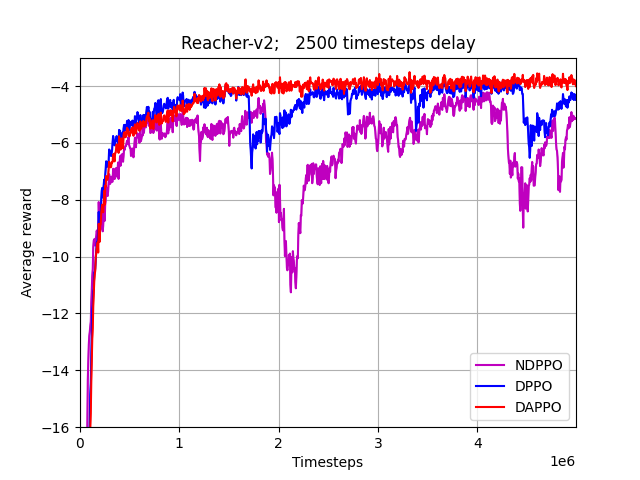
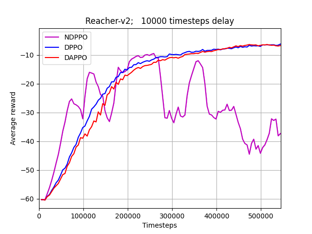
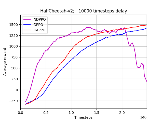
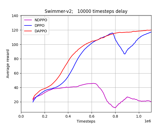
Figure 3: Instability of NDPPO: The learning curve of NDPPO vs DAPPO and DPPO under various settings. Plots show reward over a single run. x-axis is the number of timesteps until massive drop in performance (or up to 5M)

.

F.2 Additional Experiments – Instability of NDPPO

We conducted experiments to show that NDPPO is an unstable algorithm. Note that $\pi^{\theta^{k-d}}(a_{h}^{k-d}\mid s_{h}^{k-d})$ is not likely to be very small since $a_{h}^{k-d}$ was sampled from $\pi^{\theta^{k-d}}(\cdot\mid s_{h}^{k-d})$. On the other hand, $\pi^{\theta^{k}}(a_{h}^{k-d}\mid s_{h}^{k-d})$ may be effectively $0$ if the probability to choose $a_{h}^{k-d}$ has decreased dramatically between time $k-d$ and time $k$. This emphasizes that NDPPO (described in Section 5) does not only optimize over a biased objective, but is also highly unstable since the gradient of $L^{k}_{ND}(\theta)$ is inversely proportional to $\pi^{\theta^{k}}(a_{h}^{k-d}\mid s_{h}^{k-d})$. To demonstrate this phenomena, we present in Fig. 3 a few runs of NDPPO (compared to DPPO and DAPPO) under various settings. In some cases, such as in the Swimmer-v2 environment, NDPPO is not able to improve the policy due to the large bias of its estimator. In other cases, such as the Reacher-v2 or HalfCheetah-v2 environments, the learning curve initially behaves similarly to DAPPO and DPPO, and sometimes even slightly better. This is due to the fact that $\pi^{\theta^{k}}(a_{h}^{k-d}\mid s_{h}^{k-d})$ is likely to be smaller then $\pi^{\theta^{k-d}}(a_{h}^{k-d}\mid s_{h}^{k-d})$, leading to larger updates (compared to DPPO and DAPPO). However, at some point, the NDPPO’s learning curve becomes much noisier due to the dramatic updates whenever $\pi^{\theta^{k}}(a_{h}^{k-d}\mid s_{h}^{k-d})\approx 0$. This may results in an unrecoverable drop in performance even when the delay is small (as presented in Fig. 3), and in general, it gives an unstable algorithm with huge variance. DAPPO naturally avoids this issue by taking the maximum between $\pi^{\theta^{k}}(a_{h}^{k-d}\mid s_{h}^{k-d})$ and $\pi^{\theta^{k-d}}(a_{h}^{k-d}\mid s_{h}^{k-d})$.

F.3 Additional Experiments – Drop in Performance as Delay Length Increases

We conducted experiments to exhibit the drop in performance that occurs when delay length increases. Fig. 4 compares the training curves of DPPO vs DAPPO with different lengths of $\tilde{d}\in\{10000,25000,50000,75000,100000\}$, alongside the training curve of PPO without delay. As expected, when the delay is relatively small (e.g., $\tilde{d}=10000$), there is no significant difference between learning with or without delayed feedback. As the delay becomes larger, the performance of all algorithms drops (but at different rates).

One exception is HalfCheetah-v2 where even for small delay performance drops. However, this is mainly due to the fact that the performance across different seeds is very noisy. Specifically, in 3 out of the 5 seeds, PPO without delays converges to a local maxima which has average reward of $\approx 1500$ (similar to DPPO and DAPPO with sufficiently large delay). In the two other seeds it converges to a much better policy, which explains the large std in these graphs.

Whenever the delay becomes sufficiently large ($\sim 25K-50K$), there is a massive drop in the performance. This emphasize the great challenge that online algorithms need to face in the presence of delays. Namely, the algorithm updates its current policy based on estimated advantage function of a very different policy than the current one. This is also the point where the way we estimate the advantage function becomes important and the difference between DPPO and DAPPO becomes much more significant.

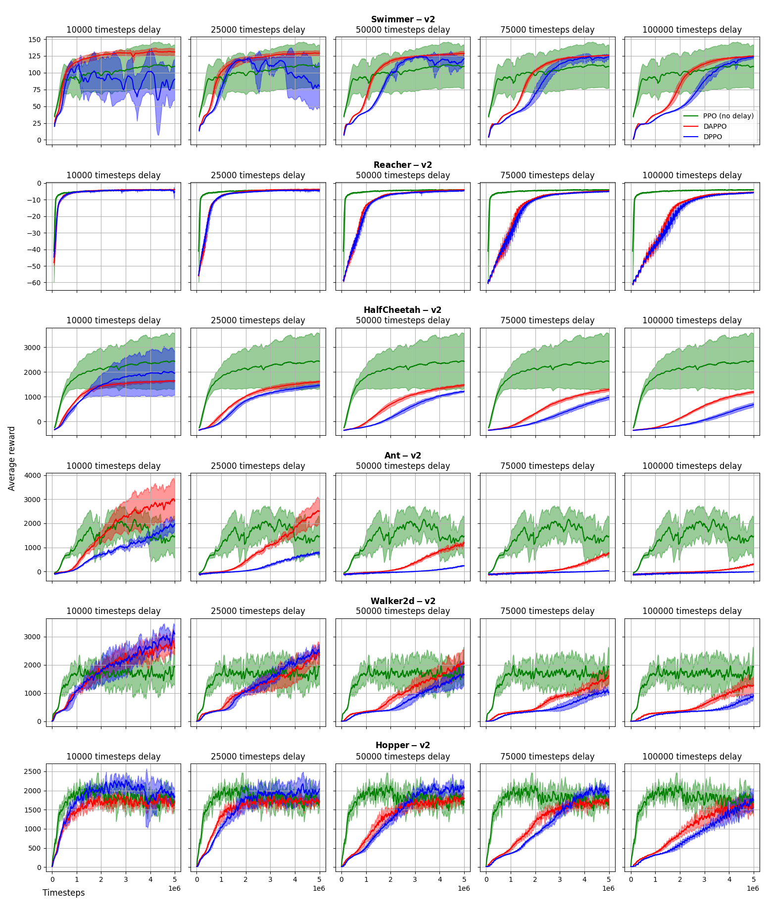
Figure 4: Training curves in different enviorments and different fixed delay length: DAPPO vs DPPO with different delay, alongside PPO without delays. Plots show average reward and std over 5 seeds. x-axis is number of timesteps up to 5M.

References

- Abbasi-Yadkori et al. (2019) Abbasi-Yadkori, Y., Bartlett, P., Bhatia, K., Lazic, N., Szepesvari, C., and Weisz, G. Politex: Regret bounds for policy iteration using expert prediction. In International Conference on Machine Learning, pp. 3692–3702. PMLR, 2019.
- Agarwal & Duchi (2012) Agarwal, A. and Duchi, J. C. Distributed delayed stochastic optimization. In 2012 IEEE 51st IEEE Conference on Decision and Control (CDC), pp. 5451–5452. IEEE, 2012.
- Agarwal et al. (2020) Agarwal, A., Kakade, S. M., Lee, J. D., and Mahajan, G. Optimality and approximation with policy gradient methods in markov decision processes. In Conference on Learning Theory, pp. 64–66. PMLR, 2020.
- Ayoub et al. (2020) Ayoub, A., Jia, Z., Szepesvari, C., Wang, M., and Yang, L. Model-based reinforcement learning with value-targeted regression. In International Conference on Machine Learning, pp. 463–474. PMLR, 2020.
- Azar et al. (2017) Azar, M. G., Osband, I., and Munos, R. Minimax regret bounds for reinforcement learning. In Proceedings of the 34th International Conference on Machine Learning-Volume 70, pp. 263–272. JMLR. org, 2017.
- Beygelzimer et al. (2011) Beygelzimer, A., Langford, J., Li, L., Reyzin, L., and Schapire, R. Contextual bandit algorithms with supervised learning guarantees. In Proceedings of the Fourteenth International Conference on Artificial Intelligence and Statistics, pp. 19–26. JMLR Workshop and Conference Proceedings, 2011.
- Bistritz et al. (2019) Bistritz, I., Zhou, Z., Chen, X., Bambos, N., and Blanchet, J. Online exp3 learning in adversarial bandits with delayed feedback. In Advances in Neural Information Processing Systems, pp. 11349–11358, 2019.
- Bistritz et al. (2021) Bistritz, I., Zhou, Z., Chen, X., Bambos, N., and Blanchet, J. No discounted-regret learning in adversarial bandits with delays. arXiv preprint arXiv:2103.04550, 2021.
- Cai et al. (2020) Cai, Q., Yang, Z., Jin, C., and Wang, Z. Provably efficient exploration in policy optimization. In International Conference on Machine Learning, pp. 1283–1294. PMLR, 2020.
- Cesa-Bianchi et al. (2016) Cesa-Bianchi, N., Gentile, C., Mansour, Y., and Minora, A. Delay and cooperation in nonstochastic bandits. In Conference on Learning Theory, pp. 605–622, 2016.
- Cesa-Bianchi et al. (2018) Cesa-Bianchi, N., Gentile, C., and Mansour, Y. Nonstochastic bandits with composite anonymous feedback. In Conference On Learning Theory, pp. 750–773, 2018.
- Cesa-Bianchi et al. (2019) Cesa-Bianchi, N., Gentile, C., and Mansour, Y. Delay and cooperation in nonstochastic bandits. The Journal of Machine Learning Research, 20(1):613–650, 2019.
- Changuel et al. (2012) Changuel, N., Sayadi, B., and Kieffer, M. Online learning for qoe-based video streaming to mobile receivers. In 2012 IEEE Globecom Workshops, pp. 1319–1324. IEEE, 2012.
- Chen et al. (2020a) Chen, B., Xu, M., Liu, Z., Li, L., and Zhao, D. Delay-aware multi-agent reinforcement learning. arXiv preprint arXiv:2005.05441, 2020a.
- Chen & Luo (2021) Chen, L. and Luo, H. Finding the stochastic shortest path with low regret: The adversarial cost and unknown transition case. arXiv preprint arXiv:2102.05284, 2021.
- Chen et al. (2020b) Chen, L., Luo, H., and Wei, C.-Y. Minimax regret for stochastic shortest path with adversarial costs and known transition. arXiv preprint arXiv:2012.04053, 2020b.
- Chen et al. (2021) Chen, L., Jafarnia-Jahromi, M., Jain, R., and Luo, H. Implicit finite-horizon approximation and efficient optimal algorithms for stochastic shortest path. Advances in Neural Information Processing Systems, 2021.
- Chen et al. (2022a) Chen, L., Jain, R., and Luo, H. Improved no-regret algorithms for stochastic shortest path with linear mdp. In International Conference on Machine Learning, pp. 3204–3245. PMLR, 2022a.
- Chen et al. (2022b) Chen, L., Luo, H., and Rosenberg, A. Policy optimization for stochastic shortest path. In Loh, P. and Raginsky, M. (eds.), Conference on Learning Theory, 2-5 July 2022, London, UK, volume 178 of Proceedings of Machine Learning Research, pp. 982–1046. PMLR, 2022b.
- Cohen et al. (2021a) Cohen, A., Daniely, A., Drori, Y., Koren, T., and Schain, M. Asynchronous stochastic optimization robust to arbitrary delays. In Ranzato, M., Beygelzimer, A., Dauphin, Y. N., Liang, P., and Vaughan, J. W. (eds.), Advances in Neural Information Processing Systems 34: Annual Conference on Neural Information Processing Systems 2021, NeurIPS 2021, December 6-14, 2021, virtual, pp. 9024–9035, 2021a.
- Cohen et al. (2021b) Cohen, A., Efroni, Y., Mansour, Y., and Rosenberg, A. Minimax regret for stochastic shortest path. Advances in Neural Information Processing Systems, 34, 2021b.
- Dai et al. (2022) Dai, Y., Luo, H., and Chen, L. Follow-the-perturbed-leader for adversarial markov decision processes with bandit feedback. arXiv preprint arXiv:2205.13451, 2022.
- Dai et al. (2023) Dai, Y., Luo, H., Wei, C.-Y., and Zimmert, J. Refined regret for adversarial mdps with linear function approximation. arXiv preprint arXiv:2301.12942, 2023.
- Dann et al. (2017) Dann, C., Lattimore, T., and Brunskill, E. Unifying pac and regret: Uniform pac bounds for episodic reinforcement learning. In Advances in Neural Information Processing Systems, pp. 5713–5723, 2017.
- Derman et al. (2021) Derman, E., Dalal, G., and Mannor, S. Acting in delayed environments with non-stationary markov policies. In 9th International Conference on Learning Representations, ICLR 2021, Virtual Event, Austria, May 3-7, 2021, 2021.
- Dudik et al. (2011) Dudik, M., Hsu, D., Kale, S., Karampatziakis, N., Langford, J., Reyzin, L., and Zhang, T. Efficient optimal learning for contextual bandits. In Proceedings of the Twenty-Seventh Conference on Uncertainty in Artificial Intelligence, pp. 169–178, 2011.
- Efroni et al. (2019) Efroni, Y., Merlis, N., Ghavamzadeh, M., and Mannor, S. Tight regret bounds for model-based reinforcement learning with greedy policies. In Wallach, H. M., Larochelle, H., Beygelzimer, A., d’Alché-Buc, F., Fox, E. B., and Garnett, R. (eds.), Advances in Neural Information Processing Systems 32: Annual Conference on Neural Information Processing Systems 2019, NeurIPS 2019, 8-14 December 2019, Vancouver, BC, Canada, pp. 12203–12213, 2019.
- Even-Dar et al. (2009) Even-Dar, E., Kakade, S. M., and Mansour, Y. Online markov decision processes. Mathematics of Operations Research, 34(3):726–736, 2009.
- Freund & Schapire (1997) Freund, Y. and Schapire, R. E. A decision-theoretic generalization of on-line learning and an application to boosting. Journal of computer and system sciences, 55(1):119–139, 1997.
- Gael et al. (2020) Gael, M. A., Vernade, C., Carpentier, A., and Valko, M. Stochastic bandits with arm-dependent delays. In International Conference on Machine Learning, pp. 3348–3356. PMLR, 2020.
- Gu et al. (2017) Gu, S., Holly, E., Lillicrap, T., and Levine, S. Deep reinforcement learning for robotic manipulation with asynchronous off-policy updates. In 2017 IEEE international conference on robotics and automation (ICRA), pp. 3389–3396. IEEE, 2017.
- Gyorgy & Joulani (2021) Gyorgy, A. and Joulani, P. Adapting to delays and data in adversarial multi-armed bandits. In International Conference on Machine Learning, pp. 3988–3997. PMLR, 2021.
- Haarnoja et al. (2018) Haarnoja, T., Zhou, A., Abbeel, P., and Levine, S. Soft actor-critic: Off-policy maximum entropy deep reinforcement learning with a stochastic actor. In International Conference on Machine Learning, pp. 1861–1870, 2018.
- He et al. (2022) He, J., Zhou, D., and Gu, Q. Near-optimal policy optimization algorithms for learning adversarial linear mixture mdps. In Camps-Valls, G., Ruiz, F. J. R., and Valera, I. (eds.), Proceedings of The 25th International Conference on Artificial Intelligence and Statistics, volume 151 of Proceedings of Machine Learning Research, pp. 4259–4280. PMLR, 28–30 Mar 2022.
- Howson et al. (2021) Howson, B., Pike-Burke, C., and Filippi, S. Delayed feedback in episodic reinforcement learning. arXiv preprint arXiv:2111.07615, 2021.
- Howson et al. (2022) Howson, B., Pike-Burke, C., and Filippi, S. Delayed feedback in generalised linear bandits revisited. arXiv preprint arXiv:2207.10786, 2022.
- Ito et al. (2020) Ito, S., Hatano, D., Sumita, H., Takemura, K., Fukunaga, T., Kakimura, N., and Kawarabayashi, K.-I. Delay and cooperation in nonstochastic linear bandits. Advances in Neural Information Processing Systems, 33:4872–4883, 2020.
- Jaksch et al. (2010) Jaksch, T., Ortner, R., and Auer, P. Near-optimal regret bounds for reinforcement learning. Journal of Machine Learning Research, 11(4), 2010.
- Jin et al. (2018) Jin, C., Allen-Zhu, Z., Bubeck, S., and Jordan, M. I. Is q-learning provably efficient? In Advances in Neural Information Processing Systems, pp. 4863–4873, 2018.
- Jin et al. (2020a) Jin, C., Jin, T., Luo, H., Sra, S., and Yu, T. Learning adversarial markov decision processes with bandit feedback and unknown transition. In International Conference on Machine Learning, pp. 4860–4869. PMLR, 2020a.
- Jin et al. (2020b) Jin, C., Yang, Z., Wang, Z., and Jordan, M. I. Provably efficient reinforcement learning with linear function approximation. In Conference on Learning Theory, pp. 2137–2143, 2020b.
- Jin & Luo (2020) Jin, T. and Luo, H. Simultaneously learning stochastic and adversarial episodic mdps with known transition. Advances in neural information processing systems, 2020.
- Jin et al. (2021) Jin, T., Huang, L., and Luo, H. The best of both worlds: stochastic and adversarial episodic mdps with unknown transition. Advances in Neural Information Processing Systems, 2021.
- Jin et al. (2022) Jin, T., Lancewicki, T., Luo, H., Mansour, Y., and Rosenberg, A. Near-optimal regret for adversarial mdp with delayed bandit feedback. arXiv preprint arXiv:2201.13172, 2022.
- Kakade & Langford (2002) Kakade, S. and Langford, J. Approximately optimal approximate reinforcement learning. In In Proc. 19th International Conference on Machine Learning. Citeseer, 2002.
- Kakade (2001) Kakade, S. M. A natural policy gradient. Advances in neural information processing systems, 14:1531–1538, 2001.
- Katsikopoulos & Engelbrecht (2003) Katsikopoulos, K. V. and Engelbrecht, S. E. Markov decision processes with delays and asynchronous cost collection. IEEE transactions on automatic control, 48(4):568–574, 2003.
- Kingma & Ba (2014) Kingma, D. P. and Ba, J. Adam: A method for stochastic optimization. arXiv preprint arXiv:1412.6980, 2014.
- Lancewicki et al. (2021) Lancewicki, T., Segal, S., Koren, T., and Mansour, Y. Stochastic multi-armed bandits with unrestricted delay distributions. In Proceedings of the 38th International Conference on Machine Learning, ICML 2021, 18-24 July 2021, Virtual Event, pp. 5969–5978. PMLR, 2021.
- Lancewicki et al. (2022a) Lancewicki, T., Rosenberg, A., and Mansour, Y. Cooperative online learning in stochastic and adversarial mdps. In Chaudhuri, K., Jegelka, S., Song, L., Szepesvári, C., Niu, G., and Sabato, S. (eds.), International Conference on Machine Learning, ICML 2022, 17-23 July 2022, Baltimore, Maryland, USA, volume 162 of Proceedings of Machine Learning Research, pp. 11918–11968. PMLR, 2022a.
- Lancewicki et al. (2022b) Lancewicki, T., Rosenberg, A., and Mansour, Y. Learning adversarial markov decision processes with delayed feedback. In Proceedings of the AAAI Conference on Artificial Intelligence, volume 36, pp. 7281–7289, 2022b.
- Levine & Koltun (2013) Levine, S. and Koltun, V. Guided policy search. In International conference on machine learning, pp. 1–9. PMLR, 2013.
- Levine et al. (2016) Levine, S., Finn, C., Darrell, T., and Abbeel, P. End-to-end training of deep visuomotor policies. The Journal of Machine Learning Research, 17(1):1334–1373, 2016.
- Lillicrap et al. (2015) Lillicrap, T. P., Hunt, J. J., Pritzel, A., Heess, N., Erez, T., Tassa, Y., Silver, D., and Wierstra, D. Continuous control with deep reinforcement learning. arXiv preprint arXiv:1509.02971, 2015.
- Liu et al. (2014) Liu, S., Wang, X., and Liu, P. X. Impact of communication delays on secondary frequency control in an islanded microgrid. IEEE Transactions on Industrial Electronics, 62(4):2021–2031, 2014.
- Luo et al. (2021) Luo, H., Wei, C.-Y., and Lee, C.-W. Policy optimization in adversarial mdps: Improved exploration via dilated bonuses. Advances in Neural Information Processing Systems, 34, 2021.
- Mahmood et al. (2018) Mahmood, A. R., Korenkevych, D., Komer, B. J., and Bergstra, J. Setting up a reinforcement learning task with a real-world robot. In 2018 IEEE/RSJ International Conference on Intelligent Robots and Systems (IROS), pp. 4635–4640. IEEE, 2018.
- Masoudian et al. (2022) Masoudian, S., Zimmert, J., and Seldin, Y. A best-of-both-worlds algorithm for bandits with delayed feedback. arXiv preprint arXiv:2206.14906, 2022.
- Min et al. (2022) Min, Y., He, J., Wang, T., and Gu, Q. Learning stochastic shortest path with linear function approximation. In International Conference on Machine Learning, pp. 15584–15629. PMLR, 2022.
- Neu (2015) Neu, G. Explore no more: Improved high-probability regret bounds for non-stochastic bandits. Advances in Neural Information Processing Systems, 28:3168–3176, 2015.
- Neu & Olkhovskaya (2021) Neu, G. and Olkhovskaya, J. Online learning in mdps with linear function approximation and bandit feedback. Advances in Neural Information Processing Systems, 34:10407–10417, 2021.
- Neu et al. (2010a) Neu, G., György, A., and Szepesvári, C. The online loop-free stochastic shortest-path problem. In COLT 2010 - The 23rd Conference on Learning Theory, Haifa, Israel, June 27-29, 2010, pp. 231–243, 2010a.
- Neu et al. (2010b) Neu, G., György, A., and Szepesvári, C. The online loop-free stochastic shortest-path problem. In Conference on Learning Theory (COLT), pp. 231–243, 2010b.
- Neu et al. (2012) Neu, G., György, A., and Szepesvári, C. The adversarial stochastic shortest path problem with unknown transition probabilities. In Proceedings of the Fifteenth International Conference on Artificial Intelligence and Statistics, (AISTATS), pp. 805–813, 2012.
- Neu et al. (2014) Neu, G., György, A., Szepesvári, C., and Antos, A. Online Markov Decision Processes under bandit feedback. IEEE Trans. Automat. Contr., 59(3):676–691, 2014.
- Pike-Burke et al. (2018) Pike-Burke, C., Agrawal, S., Szepesvari, C., and Grunewalder, S. Bandits with delayed, aggregated anonymous feedback. In International Conference on Machine Learning, pp. 4105–4113. PMLR, 2018.
- Quanrud & Khashabi (2015) Quanrud, K. and Khashabi, D. Online learning with adversarial delays. Advances in neural information processing systems, 28:1270–1278, 2015.
- Raffin et al. (2021) Raffin, A., Hill, A., Gleave, A., Kanervisto, A., Ernestus, M., and Dormann, N. Stable-baselines3: Reliable reinforcement learning implementations. Journal of Machine Learning Research, 2021.
- Rosenberg & Mansour (2019a) Rosenberg, A. and Mansour, Y. Online stochastic shortest path with bandit feedback and unknown transition function. In Advances in Neural Information Processing Systems, pp. 2209–2218, 2019a.
- Rosenberg & Mansour (2019b) Rosenberg, A. and Mansour, Y. Online convex optimization in adversarial markov decision processes. In International Conference on Machine Learning, pp. 5478–5486. PMLR, 2019b.
- Rosenberg & Mansour (2021a) Rosenberg, A. and Mansour, Y. Oracle-efficient regret minimization in factored mdps with unknown structure. In Ranzato, M., Beygelzimer, A., Dauphin, Y. N., Liang, P., and Vaughan, J. W. (eds.), Advances in Neural Information Processing Systems 34: Annual Conference on Neural Information Processing Systems 2021, NeurIPS 2021, December 6-14, 2021, virtual, pp. 11148–11159, 2021a.
- Rosenberg & Mansour (2021b) Rosenberg, A. and Mansour, Y. Stochastic shortest path with adversarially changing costs. In Zhou, Z. (ed.), Proceedings of the Thirtieth International Joint Conference on Artificial Intelligence, IJCAI 2021, Virtual Event / Montreal, Canada, 19-27 August 2021, pp. 2936–2942. ijcai.org, 2021b.
- Rosenberg et al. (2020) Rosenberg, A., Cohen, A., Mansour, Y., and Kaplan, H. Near-optimal regret bounds for stochastic shortest path. In International Conference on Machine Learning, pp. 8210–8219. PMLR, 2020.
- Schuitema et al. (2010) Schuitema, E., Buşoniu, L., Babuška, R., and Jonker, P. Control delay in reinforcement learning for real-time dynamic systems: a memoryless approach. In 2010 IEEE/RSJ International Conference on Intelligent Robots and Systems, pp. 3226–3231. IEEE, 2010.
- Schulman et al. (2015) Schulman, J., Levine, S., Abbeel, P., Jordan, M., and Moritz, P. Trust region policy optimization. In International conference on machine learning, pp. 1889–1897, 2015.
- Schulman et al. (2017) Schulman, J., Wolski, F., Dhariwal, P., Radford, A., and Klimov, O. Proximal policy optimization algorithms. arXiv preprint arXiv:1707.06347, 2017.
- Shani et al. (2020a) Shani, L., Efroni, Y., and Mannor, S. Adaptive trust region policy optimization: Global convergence and faster rates for regularized mdps. In The Thirty-Fourth AAAI Conference on Artificial Intelligence, AAAI 2020, The Thirty-Second Innovative Applications of Artificial Intelligence Conference, IAAI 2020, The Tenth AAAI Symposium on Educational Advances in Artificial Intelligence, EAAI 2020, New York, NY, USA, February 7-12, 2020, pp. 5668–5675. AAAI Press, 2020a.
- Shani et al. (2020b) Shani, L., Efroni, Y., Rosenberg, A., and Mannor, S. Optimistic policy optimization with bandit feedback. In International Conference on Machine Learning, pp. 8604–8613. PMLR, 2020b.
- Sherman et al. (2023) Sherman, U., Koren, T., and Mansour, Y. Improved regret for efficient online reinforcement learning with linear function approximation. arXiv preprint arXiv:2301.13087, 2023.
- Sutton & Barto (2018) Sutton, R. S. and Barto, A. G. Reinforcement learning: An introduction. MIT press, 2018.
- Sutton et al. (1999) Sutton, R. S., McAllester, D., Singh, S., and Mansour, Y. Policy gradient methods for reinforcement learning with function approximation. Advances in neural information processing systems, 12, 1999.
- Tarbouriech et al. (2020) Tarbouriech, J., Garcelon, E., Valko, M., Pirotta, M., and Lazaric, A. No-regret exploration in goal-oriented reinforcement learning. In International Conference on Machine Learning, pp. 9428–9437. PMLR, 2020.
- Tarbouriech et al. (2021) Tarbouriech, J., Zhou, R., Du, S. S., Pirotta, M., Valko, M., and Lazaric, A. Stochastic shortest path: Minimax, parameter-free and towards horizon-free regret. Advances in Neural Information Processing Systems, 34, 2021.
- Thune et al. (2019) Thune, T. S., Cesa-Bianchi, N., and Seldin, Y. Nonstochastic multiarmed bandits with unrestricted delays. In Advances in Neural Information Processing Systems, pp. 6541–6550, 2019.
- Todorov et al. (2012) Todorov, E., Erez, T., and Tassa, Y. Mujoco: A physics engine for model-based control. In 2012 IEEE/RSJ international conference on intelligent robots and systems, pp. 5026–5033. IEEE, 2012.
- Tomar et al. (2022) Tomar, M., Shani, L., Efroni, Y., and Ghavamzadeh, M. Mirror descent policy optimization. In The Tenth International Conference on Learning Representations, ICLR 2022, Virtual Event, April 25-29, 2022, 2022.
- Van Der Hoeven & Cesa-Bianchi (2022) Van Der Hoeven, D. and Cesa-Bianchi, N. Nonstochastic bandits and experts with arm-dependent delays. In International Conference on Artificial Intelligence and Statistics. PMLR, 2022.
- Vernade et al. (2017) Vernade, C., Cappé, O., and Perchet, V. Stochastic bandit models for delayed conversions. In Conference on Uncertainty in Artificial Intelligence, 2017.
- Vernade et al. (2020) Vernade, C., Carpentier, A., Lattimore, T., Zappella, G., Ermis, B., and Brueckner, M. Linear bandits with stochastic delayed feedback. In International Conference on Machine Learning, pp. 9712–9721. PMLR, 2020.
- Vial et al. (2022) Vial, D., Parulekar, A., Shakkottai, S., and Srikant, R. Regret bounds for stochastic shortest path problems with linear function approximation. In International Conference on Machine Learning, pp. 22203–22233. PMLR, 2022.
- Walsh et al. (2009) Walsh, T. J., Nouri, A., Li, L., and Littman, M. L. Learning and planning in environments with delayed feedback. Autonomous Agents and Multi-Agent Systems, 18(1):83, 2009.
- Wei et al. (2021) Wei, C.-Y., Jahromi, M. J., Luo, H., and Jain, R. Learning infinite-horizon average-reward mdps with linear function approximation. In International Conference on Artificial Intelligence and Statistics, pp. 3007–3015. PMLR, 2021.
- Yang & Wang (2019) Yang, L. and Wang, M. Sample-optimal parametric q-learning using linearly additive features. In International Conference on Machine Learning, pp. 6995–7004. PMLR, 2019.
- Zanette et al. (2020a) Zanette, A., Brandfonbrener, D., Brunskill, E., Pirotta, M., and Lazaric, A. Frequentist regret bounds for randomized least-squares value iteration. In International Conference on Artificial Intelligence and Statistics, pp. 1954–1964, 2020a.
- Zanette et al. (2020b) Zanette, A., Lazaric, A., Kochenderfer, M., and Brunskill, E. Learning near optimal policies with low inherent bellman error. In International Conference on Machine Learning, pp. 10978–10989. PMLR, 2020b.
- Zhou & Gu (2022) Zhou, D. and Gu, Q. Computationally efficient horizon-free reinforcement learning for linear mixture mdps. arXiv preprint arXiv:2205.11507, 2022.
- Zhou et al. (2021) Zhou, D., Gu, Q., and Szepesvari, C. Nearly minimax optimal reinforcement learning for linear mixture markov decision processes. In Conference on Learning Theory, pp. 4532–4576. PMLR, 2021.
- Zhou et al. (2019) Zhou, Z., Xu, R., and Blanchet, J. Learning in generalized linear contextual bandits with stochastic delays. In Advances in Neural Information Processing Systems, pp. 5197–5208, 2019.
- Zimin & Neu (2013) Zimin, A. and Neu, G. Online learning in episodic markovian decision processes by relative entropy policy search. In Advances in Neural Information Processing Systems 26: 27th Annual Conference on Neural Information Processing Systems 2013. Proceedings of a meeting held December 5-8, 2013, Lake Tahoe, Nevada, United States, pp. 1583–1591, 2013.
- Zimmert & Seldin (2020) Zimmert, J. and Seldin, Y. An optimal algorithm for adversarial bandits with arbitrary delays. In International Conference on Artificial Intelligence and Statistics, pp. 3285–3294. PMLR, 2020.