Understanding and Improving Model Averaging in Federated Learning on Heterogeneous Data

Abstract

Model averaging is a widely adopted technique in federated learning (FL) that aggregates multiple client models to obtain a global model. Remarkably, model averaging in FL can yield a superior global model, even when client models are trained with non-convex objective functions and on heterogeneous local datasets. However, the rationale behind its success remains poorly understood. To shed light on this issue, we first visualize the loss landscape of FL over client and global models to illustrate their geometric properties. The visualization shows that the client models encompass the global model within a common basin, and interestingly, the global model may deviate from the bottom of the basin while still outperforming the client models. To gain further insights into model averaging in FL, we decompose the expected loss of the global model into five factors related to the client models. Specifically, our analysis reveals that the loss of the global model after early training mainly arises from i) the client model’s loss on non-overlapping data between client datasets and the global dataset and ii) the maximum distance between the global and client models. Based on these findings from our loss landscape visualization and loss decomposition, we propose utilizing iterative moving averaging (IMA) on the global model at the late training phase to reduce its deviation from the expected minimum, while constraining client exploration to limit the maximum distance between the global and client models. Our experiments demonstrate that incorporating IMA into existing FL methods significantly improves their accuracy and training speed on various heterogeneous data setups of benchmark datasets.

1 Introduction

Federated learning (FL) [1] enables clients to collaboratively train a machine learning model while keeping their data decentralized to protect privacy. One of the primary challenges in FL is the heterogeneous data across clients, which diverges client models and deteriorates the performance of FL [2]. Despite this challenge, numerous works have effectively integrated FL into the artificial intelligence (AI) services of large-scale networks with enormous data to ensure the smooth operation of these networks, including the Internet of Things (IoT) [3, 4], wireless networks [5, 6], mobile networks [7, 8] and vehicular networks [9]. As per [10], the empirical success suggests that FL may surpass its theoretical expectations.

A common view of the empirical success of FL is that federated model averaging (FMA) mitigates the effect of heterogeneous data in FL, as per [11]. Model averaging, first introduced in [12], is a widely used technique to reduce communication overhead [13] and the variance of gradients [14] in distributed/decentralized learning [15] by periodically averaging models trained over parallel workers with homogeneous data. In this work, we refer to model averaging in FL with heterogeneous data as FMA to distinguish it from model averaging in other communities (e.g., distributed learning with homogeneous data). Specifically, at each round, FMA aggregates $K$ client models updated locally on heterogeneous data to obtain a global model $\mathbf{w}$ as $\mathbf{w}\leftarrow\sum_{k=1}^{K}({n_{k}}/{\sum_{k}n_{k}})\mathbf{w}_{k}$, where $\mathbf{w}_{k}$ is the $k$-th client model and $n_{k}$ is the size of the $k$-th client dataset. Surprisingly, FMA can effectively work with divergent client models and alleviate their impact on FL [10].

However, it remains unclear how FMA mitigates the effect of divergent client models and enables the global model to converge throughout the training process. Existing works, e.g., [16, 17], analyze the convergence rate of FMA-based FL under the assumption of bounded gradient dissimilarity. Specifically, these analyses use an assumed upper bound on the distance between the global and client gradients to demonstrate how heterogeneous data degrade the convergence rate of FL. However, a recent work [18] finds that the actual drift of the global gradient is significantly smaller than what is expected based on this bound, while client gradients diverge from each other. This indicates that the bound may not accurately characterize the effect of heterogeneous data on FL. Moreover, this bound neglects the overall relationship among all client gradients, as suggested in [18]. This means that the effect of FMA on FL is ignored by this bound, while FMA plays a practical role in alleviating the drift of the global gradient [11]. Therefore, a conclusive explanation of how FMA assists FL is still lacking.

To fill this gap, we first investigate the geometric properties of FMA by visualizing the loss/error landscape based on the global model and client models. Our investigation reveals that the global model is closely surrounded by client models within a common basin and consistently achieves lower test loss and error. Then, we decompose the expected loss of the global model to establish a connection between the loss of the global model and client models. Based on this connection, we analyze how the loss of the global model is affected by five factors throughout the training process, including training bias, heterogeneous bias, model-prediction variance, covariance between client models, and locality. Our visualization and decomposition demonstrate that FMA may push the global model away from the expected loss center when facing heterogeneous data. To mitigate the deviation, we employ iterative moving averaging (IMA) on global models along their optimization trajectory. By integrating IMA into various FL methods, we can effectively reduce the deviation of the global model and keep the model in a low-loss region, thereby improving the training performance.

In this work, we aim to unravel the underlying mechanism of FMA and improve it based on the properties of loss landscape and loss decomposition in FL on heterogeneous data. Our main contributions are summarized as follows:

• We investigate the dynamics of test loss and classification error landscapes over the global and client models. Through visualization of these landscapes, we observe that while achieving lower loss/error than client models, the global model is closely surrounded by client models in a common basin but may deviate from its lowest point.

• We decompose the global model loss by analyzing the bias and variance of client models on the global dataset. We demonstrate that after early training, the global model loss is dominated by the loss of client models on non-overlapping data between their datasets and the global dataset, as well as their maximum distance from the global model.

• Our loss visualization and decomposition indicate that FMA may shift the global model away from the expected point. To mitigate this deviation, we introduce IMA on global models and decay client exploration in late training stages.

• Our experiments show that IMA improves the performance of existing FL methods on various benchmark datasets, enhancing model accuracy and reducing communication costs.

The remainder of this paper is organized as follows. Section 2 reviews related works to ours. Section 3 introduces preliminaries on FL and loss landscape visualization. The loss landscape of FMA is visualized in Section 4, and we present our theoretical and empirical analysis of FMA in Section 5. Section 6 outlines our proposed method for improving FMA, while simulation results are presented in Section 7. Finally, the concluding remarks are presented in Section 8.

2 Related Works

2.1 Model Averaging

Model averaging in machine learning (ML) is a technique developed to reduce the variance of model updating by periodically averaging models trained over multiple rounds. It was first introduced to average models along the training trajectory in centralized training [12], and then widely adopted to average models over parallel workers in distributed learning [13, 14, 19]. Izmailov et al. [20] discover that a converged ML model tends to end up at the boundary rather than the center of its loss basin while maintaining low loss. To encourage convergence to the basin center, stochastic weight averaging (SWA) was proposed for averaging model weights along the optimization path in the final stage. SWA does not reinitialize training with the averaged model, thus preserving the optimization trajectory. SWA has been extended to distributed learning [21] and FL [22]. Furthermore, maintaining models with mild diversity in the model ensemble and model average [23, 24] has been shown to improve the model generalization.

A comprehensive survey [10] indicates that although FMA has achieved empirical success in FL, its underlying mechanisms remain unclear. Unlike traditional model averaging that focuses on homogeneous data, FMA needs to accommodate the challenges posed by heterogeneous data in FL [1]. Notably, despite clients optimizing non-convex ML objectives on heterogeneous local datasets, FMA consistently achieves a converged global model by aggregating divergent client models. Therefore, to understand the mechanism of FMA, we begin by analyzing its geometric properties on heterogeneous data through loss landscape visualization, followed by decomposing the expected loss.

2.2 FL on Heterogeneous Data

Heterogeneous data across clients is one of the primary challenges in FL [2]. Common solutions involve improving the local training on clients or modifying model aggregation on the server. Client-side methods typically introduce regularization to local loss functions to prevent local models from converging to their local minima instead of the FL minima. For example, regularization can be designed as the distance between client and global models in FedProx [25], the distance between feature anchors and features in FedFA [26], or the distance among client-invariance features in FedCiR [27]. However, these approaches are not based on a good understanding of how FMA performs in FL. On the other hand, server-side methods develop alternative aggregation schemes building upon FMA. For instance, before performing FMA at the server, FedNova [28] normalizes local updates to mitigate the impact of varying numbers of local updates, FedAdam and FedYogi [29] introduce adaptive momentum to mitigate updating oscillation of the global model, and FedGMA [30] applies the AND-Masked gradient update to sparsify the global model. In addition, some methods allow clients to share data with privacy guarantees, such as sharing synthesized [31] or coded data [32, 33].

While improving FL performance on heterogeneous data, analyses of existing works like [17, 25, 34, 28] mainly focus on the overall convergence of their proposed methods, rather than elucidating the success of FMA. A common assumption of these analyses is the bounded dissimilarity of client gradients [16, 28], but this assumption is overly pessimistic, as indicated in [18]. It fails to characterize the practical drift of the global model, which is much smaller after FMA on client updates than the theoretical expectation. As suggested in [11], FMA may maintain the drift close to zero on heterogeneous data, though the underlying rationale remains unclear. To fill this gap, we investigate how FMA achieves success throughout the whole training and how to improve it.

2.3 Loss Landscape Analysis

Loss landscape [35] analysis refers to the visualization and understanding of the optimization landscape of a model’s loss function. It is a common approach to provide insights into models’ convergence, generalization, and geometric properties. The loss landscape is typically visualized by plotting the loss function through low-dimensional projections along random or meaningful directions in the parameter space [36, 20, 37]. In [36], Goodfellow et al. take the first step to visualize the optimization trajectory of ML models using low-dimensional projections, enabling comparison of different optimization algorithms. In [37], the concepts of sharp and flat minima are introduced, where flat minima generally yield better generalization. Subsequently, Izmailov et al. [20] leverage landscape visualization to show that a converged ML model tends to end up at the boundary of the loss basin instead of its flatter center. In addition, sharpness aware minimization (SAM) is introduced to seek flat minima [38] and extended to domain generalization [39] and FL [22].

Regarding geometric structure, Garipov et al. [40] discover that different minima in ML models have a connected structure called mode connectivity despite the non-convex nature of the problem. Specifically, local minima can be connected through simple interpolation paths, making additional minima easier to find. This implies that local minima are not isolated but interconnected within a manifold [41]. Previous studies mainly focus on the loss landscape in centralized training with homogeneous data [35]. Meanwhile, only a few preliminary studies [42, 43] visualize the loss landscape of FL, but they do not focus on how FMA helps FL address heterogeneous data. In our work, we explore the geometric properties of FMA and visualize its loss landscape. We demonstrate that the global model may deviate from the expected point when using FMA.

2.4 Bias-variance Loss Decomposition

Bias-variance loss decomposition is a helpful concept for understanding the performance of ML models [44, 45, 46, 47]. Specifically, the expected model loss is decomposed into bias, variance, and irreducible error components. Bias quantifies the fitting capability of models on the training data, while variance reflects the models’ sensitivity to small fluctuations in training data [44]. In [46], a unified bias-variance decomposition framework for regression and classification tasks is proposed to guide model selection in the model ensemble. In the context of deep learning, Belkin et al. [48] study how ML models achieve low bias and variance via this decomposition.

Our study presents a novel decomposition of the expected loss of the FMA model into five factors, including bias, variance, covariance, and locality, to clarify its mechanism, as detailed in Section 5. This differs from the bias-variance reduction in optimization, which controls the variance of gradient updates to accelerate convergence [34]. We aim to assess how well the global model performs on the global dataset by analyzing the performance of client models on their respective local datasets. The decomposition between client and global models provides insights that align with our findings in the loss landscape analysis in Section 4.

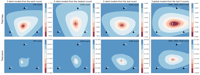
Figure 1: Visualization of the loss (top row) and classification error (bottom row) landscapes on the CIFAR-10 testset, along with three client models from the early stage (first column), middle stage (second column) and final stage (third column), as well as the visualization of three global models from the final three rounds (fourth column). The black triangles represent the location of three models in the plane, while the white cross represents their average model’s location.

3 Preliminaries

3.1 Federated Learning (FL)

3.1.1 FL Problem Formulation

We consider an FL framework with $K$ clients, each possessing its own dataset $\mathcal{D}_{k}=\{(x,y)\}\sim\mathcal{P}_{k}$ consisting of $n_{k}$ data samples, where $x$ and $y$ denote a labeled data sample and its corresponding label, respectively. The global dataset of FL is the union of all client datasets and denoted by $\mathcal{D}=\cup_{k=1}^{K}\mathcal{D}_{k}\sim\mathcal{P}$, comprising $n=\sum_{k=1}^{N}n_{k}$ data samples. Here, $\mathcal{P}_{k}$ and $\mathcal{P}$ represent the client data distribution and global data distribution, respectively. When dealing with a ML task on the global dataset $\mathcal{D}$, FL uses a finite-sum objective to minimize the expected global loss $\mathcal{L}(\mathbf{w}):=\mathbb{E}_{(x,y)\in\mathcal{D}}[l(\mathbf{w};(x,y))]$, where $l(\mathbf{w})$ denotes the global loss function for model parameters $\mathbf{w}$. As shown in [1], this objective can be reformulated as:

$$\min_{\mathbf{w}\in\mathbb{R}}\mathcal{L}(\mathbf{w})= \sum_{k=1}^{K}\frac{n_{k}}{n}\mathcal{L}_{k}(\mathbf{w})=\sum_{k=1}^{K}\frac{n_{k}}{n}\sum_{i=1}^{n_{k}}l_{k}(\mathbf{w};({x}_{i},y_{i})\in\mathcal{D}_{k}),$$ (1)

where $\mathcal{L}_{k}(\cdot)$ is the expected local loss of the $k$-th client on its local dataset $\mathcal{D}_{k}$, and $l_{k}(\mathbf{w})$ is the local loss function on $\mathbf{w}$.

An FL method called FedAvg [1] optimizes the objective (1) by averaging client models at the server in a periodic manner. In each round, the method consists of the following steps:

1. Clients update their local models $\{\mathbf{w}_{k}\}_{k=1}^{K}$ independently by minimizing their local losses $\{\mathcal{L}_{k}(\mathbf{w}_{k})\}_{k=1}^{K}$ on the local datasets $\{\mathcal{D}_{k}\}_{k=1}^{K}$;

2. Clients upload their updated models to the server;

3. The server performs FMA on the local models to calculate the new global model, i.e., $\mathbf{w}=\sum_{k=1}^{K}\frac{n_{k}}{n}\mathbf{w}_{k}$;

4. The new global model $\mathbf{w}$ is sent back to clients to initialize the next round of local training.

This process repeats until the global model converges.

3.1.2 Heterogeneous Data Problem and FMA in FL

The objective (1) assumes that the client data distribution $\mathcal{P}_{k}$ is formed by uniformly and randomly distributing the training examples from the global data distribution $\mathcal{P}$. However, the assumption does not generally hold in FL due to heterogeneous data among clients, where $\mathcal{P}_{k}\neq\mathcal{P}_{k^{\prime}}\neq\mathcal{P}$ when $k\neq k^{\prime}$. As per [2, 28, 25], FL performance can be negatively impacted by heterogeneous data, leading to a slower convergence speed and worse model generalization.

There are two common types of heterogeneous data [10]: feature distribution skew and label distribution skew, referred to as feature skew and label skew, respectively, in this work for brevity. Our work delves into the effect of these two types of heterogeneous data on FMA in FL. Suppose that the $k$-th client data distribution follows $\mathcal{P}_{k}({x},y)=\mathcal{P}_{k}({x}|y)\mathcal{P}_{k}(y)=\mathcal{P}_{k}(y|{x})\mathcal{P}_{k}({x})$, where $\mathcal{P}_{k}({x})$ and $\mathcal{P}_{k}(y)$ denote the input feature marginal distribution and label marginal distribution of the $k$-th client distribution, respectively. Specifically, label skew means that $\mathcal{P}_{k}(y)$ varies from $\mathcal{P}_{k^{\prime}}({y})$ while $\mathcal{P}_{k}({x}|y)=\mathcal{P}_{k^{\prime}}({x}|y)$ for clients $k\neq k^{\prime}$; feature skew means that $\mathcal{P}_{k}({x})$ varies from $\mathcal{P}_{k^{\prime}}({x})$ while $\mathcal{P}_{k}(y|{x})=\mathcal{P}_{k^{\prime}}(y|{x})$ for clients $k\neq k^{\prime}$.

In FL, when optimizing the objective (1) on heterogeneous data, $\mathcal{L}_{k}$ can be an arbitrarily poor approximation to $\mathcal{L}$ [1], e.g., a totally inconsistent local objective with the FL objective, potentially hindering the FL convergence. Nonetheless, FL typically outperforms its theoretical convergence expectation despite data heterogeneity [18]. For example, FedAvg shows empirical success as per [10], with FMA keeping the global model converging throughout the training process. A recent survey [49] discovers that FMA effectively balances sharing information among clients while preserving privacy. This highlights the crucial role of FMA in FedAvg. However, it remains unclear how it mitigates the impact of heterogeneous data on FL.

3.2 Loss Landscape Visualization

The loss landscape depicts the distribution of loss values throughout the model’s weight space. As per [35], exploring the loss landscape can enhance our understanding of ML problems. While it is generally difficult to visualize the landscape in high-dimensional spaces, there have been many attempts to achieve it by dimensionality reduction. This helps reveal the geometric properties of neural networks, such as flatness [40] and optimization trajectory [36]. In this work, we employ two common approaches to visualize the loss landscape of FL: 1D and 2D visualizations.

For 1D visualization, we follow [36] to draw the loss landscape in a line segment (1D) by using linear interpolation between two models $\mathbf{w}_{1}$ and $\mathbf{w}_{2}$. Specifically, given a target dataset, we evaluate the loss of different model weights along the line segment between $\mathbf{w}_{1}$ and $\mathbf{w}_{2}$, i.e., $\mathcal{L}_{[\mathbf{w}_{1},\mathbf{w}_{2}]}(\beta)=\mathcal{L}(\beta\mathbf{w}_{1}+(1-\beta)\mathbf{w}_{2})$, where $\beta$ is the interpolation coefficient of line model interpolation between $\mathbf{w}_{1}$ and $\mathbf{w}_{2}$.

For 2D visualization, we explore the loss landscape in a plane (2D) by drawing the contour based on three models according to [20]. Specifically, we take $\mathbf{w}_{1},\mathbf{w}_{2},\mathbf{w}_{3}$ to form a plane by constructing two base vectors $\mathbf{\bar{u}}=\mathbf{u}/\|\mathbf{u}\|^{2}$ and $\mathbf{\bar{v}}=\mathbf{v}/\|\mathbf{v}\|^{2}$, where $\mathbf{u}=\mathbf{w}_{2}-\mathbf{w}_{1}$ and $\mathbf{v}=(\mathbf{w}_{3}-\mathbf{w}_{1})-\left\langle\mathbf{w}_{3}-\mathbf{w}_{1},\mathbf{w}_{2}-\mathbf{w}_{1}\right\rangle/\|\mathbf{w}_{2}-\mathbf{w}_{1}\|^{2}\cdot(\mathbf{w}_{2}-\mathbf{w}_{1})$. Next, each point P in the plane, with coordinates $(a,b)$, represents a model $\mathbf{w}_{\textit{P}}=\mathbf{w}_{1}+a\cdot\mathbf{\bar{u}}+b\cdot\mathbf{\bar{v}}$. Finally, given a target dataset, we evaluate the loss $\mathcal{L}(\mathbf{w}_{\textit{P}})$ of all the points in this plane and draw the loss contour by $\{\mathcal{L}(\mathbf{w}_{\textit{P}})=c\}$, where $c$ is the contour value.

4 Loss Landscape Visualization in FL

In this section, we explore the geometric properties of FMA through 2D loss landscape visualization. As depicted in Figure 1, to construct the plane of 2D visualization, we use three client models from the same training round in the first three columns and three global models from different training rounds in the fourth column. The FL setup related to Figure 1 involves training a global model on the CIFAR-10 dataset [50] across 100 clients over 400 rounds. To introduce data heterogeneity, each client dataset contains two class shards of CIFAR-10, following [1] (see specific setups in Table VI). In this setup, the ideal accuracy of client models on the CIFAR-10 testset is $20\%$ if clients train their models by their local datasets. Additional visualization results for various setups, including different datasets, data heterogeneity, models, and FL settings, are provided in the Appendix.

4.1 Lower Test Loss with FMA

In Figure 1, we observe that the averaged model (i.e., the white cross) of the three client models (i.e., the black triangles) is consistently located at the regions with lower test loss and classification error than individual client models. This implies that FMA can effectively aggregate local information from different clients into the global model. Furthermore, the first three columns of Figure 1 correspond to three different training stages. As training progresses, since the newly-aggregated global model re-initiates client models with lower loss, FMA prevents them from over-fitting on their respective datasets. Meanwhile, FMA leverages client models with lower loss to anchor the global model more precisely in a lower-loss landscape area. This indicates that FMA effectively prevents the aggregation of over-fitting information into the global model.

Moreover, we observe a bias between the white cross and the lowest loss/error point in the first three columns of Figure 1. This bias can be caused by the deviation between the averaged models (i.e., the white cross) and the global model or between the global model and its expected model. To further investigate this bias, we visualize the loss/error landscape of global models obtained from the final three rounds (i.e., the 398th, 399th, and 400th rounds) in the fourth column of Figure 1. A bias exists between the global models (i.e., the black triangle) and the lowest point, similar to the bias observed in the landscape visualization over client models, while their averaged model (i.e., the white cross) is closer to the lowest point. This reveals that the only performing FMA on client models may fail to achieve the expected global model. In Section 6, we will address the deviation of the global model aggregated by FMA from the lowest loss point.

4.2 Global Model and Client Models in a Common Basin

In Figure 1, the second row demonstrates that the test classification errors of client models are around $80\%$. These errors almost reach the lowest classification error obtained by client models obtained through local training, indicating their proximity to local optima. Moreover, Figure 1 illustrates that the averaged model is surrounded by client models and located in the vicinity of a local optimum of the global model throughout the entire training process. Meanwhile, the distance between global and client models remains limited, as presented in Figure 3. These observations suggest that client models within a common basin closely surround the global model.

Geometrically, the test loss/error landscape in FL can be viewed as a basin, with client models reaching the wall of the basin and the global model residing at the bottom, as shown in Figure 1. This geometric property provides a novel insight into the mechanism behind FMA in FL. For example, Wang et al. [18] empirically found that the client-update drifts’ practical impact on the global model’s convergence speed is less than predicted by theoretical analysis. This observation can be explained by the geometric property as follows: Since client models reach the basin’s wall and their initial models (i.e., the global model) are closer to the bottom, the direction of client updates may radiate in all directions, especially in the late training stage. When FL performs FMA on the drifts of client updates, these drifts tend to cancel each other out, resulting in a limited impact on the global model.

5 Expected Loss Decomposition

In this section, we will analyze the relationship between the loss between the global and client models when FL performs FMA. To decompose the expected loss of the global model, we first examine the connection between FMA and the weighted-model ensemble (WENS). Next, we decompose the global model’s expected loss using this connection based on the client models’ losses. Finally, we empirically validate our decomposition analysis to demonstrate which factors dominate the global model’s loss throughout the training process.

We represent the model function of $\mathbf{w}$ as $f_{\mathbf{w}}:\mathcal{X}\rightarrow\mathcal{Y}$, where $\mathcal{X}$ and $\mathcal{Y}$ are input and output spaces, respectively. For simplicity, we focus on the mean-square error (MSE) loss in the theoretical analysis, i.e., $l(\mathbf{w};(x,y))=(y-f_{\mathbf{w}}(x))^{2}$. It is worth noting that this framework can be extended to other loss functions [46]. Due to mode connectivity of neural networks [20, 41, 51], given a model architecture $\mathcal{W}\subset\mathbb{R}^{d}$, a loss function $\mathcal{L}$ and a training dataset $\mathcal{D}_{\rm tr}$, there exists a single connected low-loss manifold containing all the minima trained on $\mathcal{D}_{\rm tr}$. In other words, there exists a subspace $\mathcal{W}_{\mathcal{D}_{\rm tr}}=\{\mathbf{w}_{\rm tr_{i}}\}\subset\mathcal{W}$, where $\mathbf{w}_{\rm tr}$ denotes a model optimized on $\mathcal{D}_{\rm tr}$. When the model $\mathbf{w}$ is uniformly distributed in $\mathcal{W}_{\mathcal{D}_{\rm tr}}$, the bias-variance decomposition of the expected loss of $\mathbf{w}$ evaluated on a test dataset $\mathcal{D}_{\rm te}$ can be expressed as per [47, 45]:

$$\mathbb{E}_{\mathbf{w}\in\mathcal{W}_{\mathcal{D}_{\rm tr}}}\mathcal{L}_{\mathcal{D}_{\rm te}}(\mathbf{w})= \mathbb{E}_{(x,y)\in\mathcal{D}_{\rm te}}[{\underbrace{\left(y-\bar{f}_{\mathcal{D}_{\rm tr}}(x)\right)}_{{\rm{Bias}}\{f|(x,y)\}}}^{2}$$ (2)

$$+\underbrace{\mathbb{E}_{\mathbf{w}\in\mathcal{W}_{\mathcal{D}_{\rm tr}}}[\left(f_{\mathbf{w}}(x)-\bar{f}_{\mathcal{D}_{\rm tr}}(x)\right)^{2}]}_{{\rm Var}\{f|x\}}],$$

where $f_{\mathbf{w}}(\cdot)$ and $\bar{f}_{\mathcal{D}_{\rm tr}}(\cdot)=\mathbb{E}_{\mathbf{w}\in\mathcal{W}_{\mathcal{D}_{\rm tr}}}[f_{\mathbf{w}}(\cdot)]$ are the model output of $\mathbf{w}$ and the expected output on $\mathcal{W}_{\mathcal{D}_{\rm tr}}$, respectively.

Since $\bar{f}_{\mathcal{D}_{\rm tr}}(\cdot)$ represents the ensemble output of all models in $\mathcal{W}_{\mathcal{D}_{\rm tr}}$, we rewrite it as a finite-sum formulation, $\bar{f}_{\mathcal{D}_{\rm tr}}(\cdot)=\frac{1}{N}\sum_{i\in[N]}f_{\mathbf{w}_{i}\in\mathcal{W}_{\mathcal{D}_{\rm tr}}}(\cdot)$. Specifically, given $\mathcal{W}_{\mathcal{D}_{\rm tr}}$ and a sample $(x,y)\in\mathcal{D}_{\rm te}$, ${\rm{Bias}}\{f|(x,y)\}$ denotes the bias between the ground truth $y$ and the ensemble output $\bar{f}_{\mathcal{D}_{\rm tr}}(x)$ and ${\rm Var}\{f|x\}$ denotes the expected MSE between $f_{\mathbf{w}}(x)$ and $\bar{f}_{\mathcal{D}_{\rm tr}}(x)$, which depends on the discrepancy between $\mathcal{D}_{\rm tr}$ and $\mathcal{D}_{\rm te}$ according to [52]. Note that the bias captures the capability of the models to fit the training data distribution $\mathcal{D}_{\rm tr}$, while the variance measures the models’ sensitivity to small fluctuations in $\mathcal{D}_{\rm tr}$.

5.1 Connection between FMA and WENS

At each round, FMA performs weighted averaging, defined as $\mathbf{w}_{\rm FMA}\leftarrow\sum_{k=1}^{K}\frac{n_{k}}{n}\mathbf{w}_{k}$, where the averaging weight depends on $n_{k}$ [1] and $n=\sum_{k}n_{k}$. According to [20], the model average is a first-order approximation of the model ensemble when the averaged models are closely located in the weight space. Based on this approximation, we incorporate weighted model averaging into the bias-variance decomposition in (2) and establish the connection between FMA and WENS in the following lemma:

Lemma 1.

(FMA and WENS. See proof in Appendix) Given $K$ models $\mathbf{\{w}_{k}\}_{k=1}^{K}$ and $n_{i}/n_{j}\neq\infty$ when $i\neq j$, we denote $\Delta_{k}=\|\mathbf{w}_{k}-\mathbf{w}_{\rm FMA}\|$ and $\Delta=\max_{k=1}^{K}\Delta_{k}$. Then, we have:

$$f_{\rm WENS}(x)-f_{\mathbf{w}_{\rm FMA}}(x)=\langle\Delta f_{\mathbf{w}_{\rm FMA}}(x),\sum_{k=1}^{K}\frac{n_{k}}{n}\Delta_{k}\rangle+O(\Delta^{2}),$$

where $f_{\rm WENS}(\cdot)=\sum_{k=1}^{K}\frac{n_{k}}{n}f_{\mathbf{w}_{k}}(\cdot)$ denotes the WENS output on $K$ models $\mathbf{\{w}_{k}\}_{k=1}^{K}$.

Lemma 1 shows that the FMA model (i.e., the global model in FL) function $f_{\rm FMA}(\cdot)$ provides a first-order approximation of the WENS function $f_{\rm WENS}(\cdot)$ of models being averaged (i.e., the client models in FL). This approximation holds true when $\Delta$ is small in FL, as verified in Figure 3.

5.2 Expected Loss Decomposition of Global Model

With Lemma 1, we can adapt the bias-variance decomposition (2) to the FL version. Specifically, the model $\mathbf{w}$ in (2) is substituted by $K$ client models $\mathbf{\{w}_{k}\}_{k=1}^{K}$, $\mathcal{D}_{\rm tr}$ and $\mathcal{D}_{\rm te}$ are modified to client datasets $\{\mathcal{D}_{k}\}_{k=1}^{K}$ and the global dataset $\mathcal{D}$, respectively. Meanwhile, $\bar{f}_{\mathcal{D}_{\rm tr}}(\cdot)=\mathbb{E}_{\mathbf{\{w}_{k}\}_{k=1}^{K}\in\prod_{k}^{K}\mathcal{W}_{\mathcal{D}_{k}}}[f_{\mathbf{\{w}_{k}\}_{k=1}^{K}}(\cdot)]=\mathbb{E}_{\mathbf{\{w}_{k}\}_{k=1}^{K}}[f_{\rm WENS}(\cdot)]$ denotes the ensemble output of the combination subspace on $K$ client models, where $\prod_{k}^{K}\mathcal{W}_{\mathcal{D}_{k}}=\mathcal{W}_{\mathcal{D}_{1}}\times\cdots\times\mathcal{W}_{\mathcal{D}_{K}}$. Then, we decompose the expected loss of $f_{\mathbf{w}_{\rm FMA}}(\cdot)$ on $\mathcal{D}$ in the following theorem:

Theorem 1.

(Loss decomposition of the global model. See proof in Appendix) Given $K$ client models $\mathbf{\{w}_{k}\}_{k=1}^{K}\in\prod_{k}^{K}\mathcal{W}_{\mathcal{D}_{k}}$, the expected loss of the global model $\mathbf{w}_{\rm FMA}$ on $\mathcal{D}$ is decomposed as:

$$\mathbb{E}_{\mathbf{\{w}_{k}\}_{k=1}^{K}} \mathcal{L}(\mathbf{{w}_{\rm FMA}})=\frac{1}{n}\sum_{(x,y)\in\mathcal{D}}[\sum_{k=1}^{K}\frac{n_{k}}{n}{\rm{TrainBias}}\{f_{\mathbf{w}_{k}}|(x,y)\}$$

$$+ \frac{n_{k}}{n}{\rm{HeterBias}}\{f_{\mathbf{w}_{k}}|(x,y)\}]^{2}+{\sum_{k=1}^{K}\frac{n_{k}^{2}}{n^{2}}{\rm Var}\{f_{\mathbf{w}_{k}}|x\}}$$

$$+ {\sum_{k}\sum_{k^{\prime}\neq k}\frac{n_{k}n_{k^{\prime}}}{n^{2}}{\rm Cov}\{f_{\mathbf{w}_{k},\mathbf{w}_{k}^{\prime}}|x\}}+O(\Delta^{2}),$$

where ${\rm{TrainBias}}\{f_{\mathbf{w}_{k}}|(x,y)\}=\mathbb{I}[{(x,y)\in\mathcal{D}_{k}}](y-\mathbb{E}_{\mathbf{w_{k}}}[f_{\mathbf{w}_{k}}(x)])$; ${\rm{HeterBias}}\{f_{\mathbf{w}_{k}}|(x,y)\}=\mathbb{I}\left[{(x,y)\in\mathcal{D}\setminus\mathcal{D}_{k}}\right]$ $(y-\mathbb{E}_{\mathbf{w_{k}}}[f_{\mathbf{w}_{k}}(x)])$; ${\rm Var}\{f_{\mathbf{w}_{k}}|x\}=\mathbb{E}_{\mathbf{{w}_{k}}}[(f_{\mathbf{w}_{k}}(x)-\mathbb{E}_{\mathbf{{w}_{k}}}[f_{\mathbf{w}_{k}}(x)])^{2}]$; ${\rm Cov}\{f_{\mathbf{w}_{k},\mathbf{w}_{k}^{\prime}}|x\}=\mathbb{E}_{\mathbf{{w}_{k}},\mathbf{{w}_{k^{\prime}}}}[(f_{\mathbf{w}_{k}}(x)-\mathbb{E}_{\mathbf{{w}_{k}}}[f_{\mathbf{w}_{k}}(x)])(f_{\mathbf{w}_{k^{\prime}}}(x)-\mathbb{E}_{\mathbf{{w}_{k^{\prime}}}}[f_{\mathbf{w}_{k^{\prime}}}(x)])]$.

In Theorem 1, the underlying meanings of the five factors are elaborated as follows:

• ${\rm{TrainBias}}\{f_{\mathbf{w}_{k}}|(x,y)\}$ captures the model fitting capability on a sample $(x,y)\in\mathcal{D}_{k}$ when given a client model ${\mathbf{w}_{k}}$ trained on $\mathcal{D}_{k}$;

• ${\rm{HeterBias}}\{f_{\mathbf{w}_{k}}|(x,y)\}$ captures the model fitting capability on a non-overlapping sample $(x,y)$ between $\mathcal{D}$ and $\mathcal{D}_{k}$ (i.e., $(x,y)\in\mathcal{D}\setminus\mathcal{D}_{k}$) when given a client model ${\mathbf{w}_{k}}$ trained on $\mathcal{D}_{k}$;

• ${\rm Var}\{f_{\mathbf{w}_{k}}|x\}$ measures the sensitivity of a client model $\mathbf{w}_{k}$ to small fluctuations in the given sample input $x\in\mathcal{D}_{k}$, which does not depend on $y$;

• ${\rm Cov}\{f_{\mathbf{w}_{k},\mathbf{w}_{k}^{\prime}}|x\}$ denotes the output correlation between client models $\mathbf{w}_{k}$ and $\mathbf{w}_{k}^{\prime}$ given the same input $x$, which does not depend on $y$;

• $O(\Delta^{2})$ represents the locality in [20, 24], i.e., the maximum distance between client and global models.

Based on these five factors, the capability of the global model on the global dataset can be quantified by the capability of client models on their local datasets. Due to the unseen samples for the client model $\mathbf{w}_{k}$ in its local dataset, ${\rm{HeterBias}}\{f_{\mathbf{w}_{k}}|(x,y)\}$ is expected to have a greater impact on the global model than ${\rm{TrainBias}}\{f_{\mathbf{w}_{k}}|(x,y)\}$. In the following, we empirically validate the effect of these factors on global model capability throughout the training.

5.3 Empirical Validation of Decomposition Analysis

The FL setup involves training a global model on CIFAR-10 across 10 clients for 400 rounds, where clients hold two class shards of CIFAR-10 for heterogeneous data setup (see specific setups in Table VI).

5.3.1 The effect of bias factor: heterogeneous bias dominates the loss of the global model after the early training

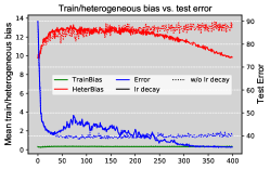
Figure 2: Train and heterogeneous biases w.r.t rounds (x-axis).

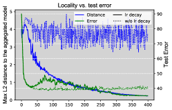
Figure 3: Locality (L2 distance) w.r.t rounds (x-axis).

Figure 2 shows that the ${\rm{TrainBias}}\{f_{\mathbf{w}_{k}}|(x,y)\}$ is effectively reduced to almost zero, which is because the number of local updates is sufficient for client models to fit their own datasets. However, heterogeneous data introduce a non-zero ${\rm{HeterBias}}\{f_{\mathbf{w}_{k}}|(x,y)\}$, which individual client struggles to address through local training due to missing samples from the global dataset. Nonetheless, due to the geometric property observed in Section 4, FMA provides an initialization point with enriched global information for client models to mitigate this bias.

Moreover, the larger the local update step, the more global information the FMA provides is forgotten, and the greater the heterogeneous bias becomes due to the catastrophic forgetting phenomenon in neural networks [53, 54]. This is validated by the cases with and without learning rate (lr) decay shown in Figure 2. We use a round-exponential decay lr to control the update size, a straightforward approach to preventing catastrophic forgetting in FL [29]. In the early phase, heterogeneous bias does not significantly impact the test classification error because the error continues to decrease even if the bias increases. However, both the error and the bias show a positive correlation in both cases. For example, after approximately 40 rounds, they both increase and decrease in the case of lr decay, and the error grows slightly with the bias in the case without lr decay.

5.3.2 The effect of locality factor: controlling the locality helps reduce the global model loss at the late training

In Figure 3, We employ the L2 distance to quantify the locality term $O(\delta^{2})$. Theorem 1 demonstrates that the test loss decreases as the maximum distance between client models and the global model, i.e., $\Delta$, reduces.

Figure 3 shows that the locality is larger in the case without lr decay, which results in a more significant test error. Before the 40th round, the test classification errors of both cases continue to decline despite an increase in the locality occurring within this period. Then, in the case of lr decay, the locality reduces while the error increases from 40 to 75 rounds. This indicates that the locality does not correlate strongly with the error during the early training. The locality stabilizes after the early training phase (i.e., the locality is upper-bounded in both cases). This further validates the proximity of client models to the global model, as discussed in Section 4.

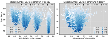
Figure 4: Test error w.r.t model number and model similarity.

5.3.3 The effect of variance factor: aggregating more client models in FMA limitedly reduces the global model loss

When the client dataset $\mathcal{D}_{k}$ would not change during the training, the variance factor $\mathbb{E}_{(x,y)\in\mathcal{D}}[{\rm Var}\{f_{\mathbf{w}_{k}}|x\}]=1/n_{k}\sum_{(x,y)\in\mathcal{D}_{k}}{\rm Var}\{f_{\mathbf{w}_{k}}|x\}$ in Theorem 1 can be viewed as a constant $V_{k}$ since ${\rm Var}\{f_{\mathbf{w}_{k}}|x\}$ depends on the discrepancy between $\mathcal{D}$ and $\mathcal{D}_{k}$. Specifically, from Theorem 1 in [52] and Proposition 2 in [24], we have the following property:

Theorem 2.

(Bounded variance.) Given a kernel regime $f_{\mathbf{w}_{k}}$ trained on client dataset $\mathcal{D}_{k}$ (of size $n_{k}$) with neural tangent kernel $K_{f_{\mathbf{w}_{k}}}$, when $\exists(\lambda_{\mathcal{D}_{k}},\epsilon)$ with $0\leq\epsilon\ll\lambda_{\mathcal{D}_{k}}$ such that $\forall x_{i}\in\mathcal{D}_{k}$, $K_{f_{\mathbf{w}_{k}}}(x_{i},x_{i})=\lambda_{\mathcal{D}_{k}}$ and $\forall x_{i},x_{j}\in\mathcal{D}_{k}$ and $i\neq j$, $|K_{f}(x_{i},x_{j})|\leq\epsilon$, the variance on the global dataset $\mathcal{D}$ is:

$$\mathbb{E}_{x\in\mathcal{D}}[{\rm Var}\{f_{\mathbf{w}_{k}}|x\}]= \frac{n_{k}}{2\lambda_{\mathcal{D}_{k}}}MMD^{2}(\mathcal{D}_{k},\mathcal{D})$$ (3)

$$+\lambda_{\mathcal{D}}-\frac{n_{k}}{2\lambda_{\mathcal{D}_{k}}}\beta_{\mathcal{D}}+O(\epsilon),$$

where $MMD(\cdot)$ is the empirical maximum mean discrepancy in the reproducing kernel Hilbert space (RKHS) of $K_{f_{\mathbf{w}_{k}}}(x_{i},x_{j})$; $\lambda_{\mathcal{D}}=\mathbb{E}_{x\in\mathcal{D}}K_{f_{\mathbf{w}_{k}}}(x,x)$ and $\beta_{\mathcal{D}}=\mathbb{E}_{x_{i},x_{j}\in\mathcal{D},i\neq j}K^{2}_{f_{\mathbf{w}_{k}}}(x_{i},x_{j})$ denote the empirical mean similarities of identical and different samples averaged over $\mathcal{D}$, respectively.

In Theorem 2, both $\lambda_{\mathcal{D}}$ and $\beta_{\mathcal{D}}$ depend exclusively on the global dataset $\mathcal{D}$ for a $f_{\mathbf{w}_{k}}$. The global dataset $\mathcal{D}$ represents the combination of all client datasets and can be viewed as a fixed dataset in FL. Consequently, $\lambda_{\mathcal{D}}$ and $\beta_{\mathcal{D}}$ can be regarded as constants that depend on $\mathcal{D}$ in Theorem 2. Therefore, Theorem 2 demonstrates that the variance term in Theorem 1 is solely associated with $MMD^{2}(\mathcal{D}_{k},\mathcal{D})$, which quantifies the distance between the client dataset $\mathcal{D}_{k}$ and the global dataset $\mathcal{D}$ in FL setups.

From Theorem 2, we have $\max_{k}\{V_{k}\}\leq\epsilon$. The whole variance term in Theorem 1 is $\sum_{k}{n_{k}^{2}}/{n^{2}}V_{k}$ and it is upper bounded by $\epsilon\sum_{k=1}^{K}{n_{k}^{2}}/{n^{2}}$. Then, FMA can keep this upper bound diminishing by averaging more client models (i.e., larger $K$ induces smaller $\sum_{k=1}^{K}{n_{k}^{2}}/{n^{2}}$) to reduce the loss of the global model when $\epsilon$ is tight for $\max_{k}\{V_{k}\}$. Figure 4 verifies this effect on FMA throughout the training process.

However, it is essential to note that the impact of the client number becomes negligible when all client models are identically distributed (i.e., client models are trained on homogeneous datasets with the same training configurations). This is because the covariance term and the sum of the variance term (i.e., ${\rm Var}\{f_{\mathbf{w}_{k}}|x\}={\rm Cov}\{f_{\mathbf{w}_{k},\mathbf{w}_{k^{\prime}}}|x\}$ when client models are identically distributed) in Theorem 1 are equal to the prediction variance of a single client model.

In summary, the variance term decreases as the number of client models being averaged in FMA increases. Nonetheless, this effect weakens as more models are incorporated.

5.3.4 The effect of covariance factor: heterogeneous data inherently results in small but lower bounded covariance

To measure the covariance factor ${\rm Cov}\{f_{\mathbf{w}_{k},\mathbf{w}_{k}^{\prime}}|x\}$, we employ the CKA similarity [50] to compute the output correlation among client models given the same input. As shown in Figure 4, heterogeneous data inherently lead to a small covariance term, especially in the case without lr decay. That is, maintaining high diversity among client models (e.g., [23, 24]) may not significantly reduce the loss of the global model. Indeed, it can even negatively impact the performance in the late training stage, as suggested by the comparison between both cases at the 400th round in Figure 4.

Furthermore, we show that the covariance term has a non-zero lower bound that depends on the maximum discrepancy across client datasets. Let $n_{i}=n_{j}$, $\forall i,j\in[K]$ (i.e., the number of client samples is the same). By ablating the impact of weighted averaging, we can further decompose the covariance term in Theorem 1 as follows:

Corollary 1.

(Lower bound of the covariance term.) For $n_{i}=n_{j}$ when $i\neq j$, the covariance term in Theorem 1 is bounded by:

$$\mathbb{E}_{(x,y)\in\mathcal{D}} (\frac{1}{K^{2}}{\sum_{k}\sum_{{k^{\prime}}}{\rm Cov}\{f_{\mathbf{w}_{k},\mathbf{w}_{k^{\prime}}}|x\}})$$ (4)

$$=\frac{1}{nK^{2}}\sum_{(x,y)\in\mathcal{D}}{\sum_{k}\sum_{{k^{\prime}}}{\rm Cov}\{f_{\mathbf{w}_{k},\mathbf{w}_{k^{\prime}}}|x\}}$$

$$\geq\frac{K-1}{nK}\sum_{(x,y)\in\mathcal{D}}\min_{(k,{k^{\prime}})}{\rm Cov}\{f_{\mathbf{w}_{k},\mathbf{w}_{k^{\prime}}}|x\},$$

where $\min_{(k,{k^{\prime}})}{\rm Cov}\{f_{\mathbf{w}_{k},\mathbf{w}_{k^{\prime}}}|x\}$ measures the maximum prediction discrepancy among all client models.

The physical meaning of $\min_{(k,{k^{\prime}})}{\rm Cov}\{f_{\mathbf{w}_{k},\mathbf{w}_{k^{\prime}}}|x\}$, when given a sample $(x,y)\in\mathcal{D}$, can be understood as follows: Firstly, ${\rm Cov}\{f_{\mathbf{w}_{k},\mathbf{w}_{k^{\prime}}}|x\}$ calculates the prediction covariance between client models $\mathbf{w}_{k}$ and $\mathbf{w}_{k^{\prime}}$. Then, $\min_{(k,{k^{\prime}})}{\rm Cov}\{f_{\mathbf{w}_{k},\mathbf{w}_{k^{\prime}}}|x\}$ find the minimal value of ${\rm Cov}\{f_{\mathbf{w}_{k},\mathbf{w}_{k^{\prime}}}|x\}$ across all client pairs $(k,k^{\prime})$, where $\forall k,k^{\prime}\in[K],k\neq k^{\prime}$. Essentially, this minimal value measures the largest diversity among client models on the given sample $(x,y)$. The maximum discrepancy across client datasets determines the diversity and remains constant since client datasets do not change in the generic FL setups.

Therefore, Corollary 1 demonstrates that the covariance term has a lower bound that depends on the maximum discrepancy across client datasets. Consequently, the effect of FMA on reducing the loss of the global model by controlling the diversity of client models is limited.

5.3.5 Summary

From the above discussion, we summarize the impact of the five factors in Theorem 1 on the loss of the global model during training as follows:

• ${\rm{TrainBias}}\{f_{\mathbf{w}_{k}}|(x,y)\}$ keeps almost zero throughout the training process;

• ${\rm{HeterBias}}$ $\{f_{\mathbf{w}_{k}}|(x,y)\}$ and $O(\Delta^{2})$ dominate the loss of the global model after the early training;

• The weighted sum of ${\rm Var}\{f_{\mathbf{w}_{k}}|x\}$ can be reduced to some extent with a large number of client models;

• ${\rm Cov}\{f_{\mathbf{w}_{k},\mathbf{w}_{k}^{\prime}}|x\}$ is too small to affect the loss of the global model.

Therefore, FMA can reduce the loss of the global model by controlling ${\rm{HeterBias}}$ $\{f_{\mathbf{w}_{k}}|(x,y)\}$ and locality $O(\Delta^{2})$, in addition to aggregating more client models.

6 Proposed Method

In this section, we will begin by discussing our motivation, i.e., to alleviate the deviation of global models in FMA. After that, we will introduce iterative moving averaging (IMA) and mild client exploration to address this deviation. Lastly, we will discuss the advantages of using IMA for FL.

6.1 Motivation: Deviation of Global Models in FMA

Theorem 1 provides a novel understanding of how the participation rate and weighted averaging lead to the deviation of global models in FMA. Specifically, the participation rate may cause the one-cohort dataset of participating clients $\mathcal{D}_{C}=\cup_{i=1}^{C}\mathcal{D}_{i}$ to deviate from the global dataset $\mathcal{D}$. In addition, the weighted averaging may assign higher weights to clients with datasets that are large but imbalanced to $\mathcal{D}$, thereby amplifying the deviation from $\mathcal{D}_{C}$ to $\mathcal{D}$. Consequently, ${\rm{HeterBias}}\{f_{\mathbf{w}_{i}}|(x,y)\}$ in Theorem 1 cannot be completely reduced since one-cohort client models $\{\mathbf{w}_{i}\}_{i}^{C}$ suffer from missing data samples $(x,y)\in\mathcal{D}\setminus\mathcal{D}_{C}$. This leads to the observed deviation of global models from the lowest point in Figure 1.

Moreover, lower loss/error points consistently exist within the interpolation of two global models from different rounds, as depicted in Figure 5(b). This observation suggests that interpolated models keep more global information than global models while keeping within a common basin. Therefore, we apply Theorem 1 to leverage the geometric properties of FMA to alleviate the deviation.

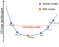
(a) Toy example

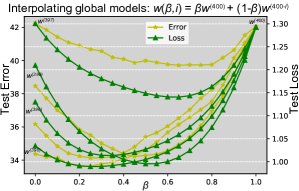
(b) Global model interpolation

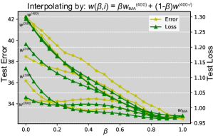
(c) Global-IMA interpolation

Figure 5: (a) A toy example of IMA; (b) interpolation among global models to validate their deviation; (c) interpolation between the IMA and global models to indicate the flatness of the IMA model.

6.2 Iterative Moving Averaging (IMA)

The missing information of one-cohort client models on $(x,y)\in\mathcal{D}\setminus\mathcal{D}_{C}$ can be compensated by utilizing historical global models. This compensation can be achieved by aggregating historical global models into the latest one, as supported by the observation in Figure 5(b). Therefore, we propose applying IMA to historical global models after sufficient training rounds instead of ignoring them in conventional FMA. Specifically, as illustrated in Figure 5(a), after $t_{s}$ rounds, the server performs FMA with IMA to obtain an averaged model from a time window of previous rounds as:

$$\mathbf{w}_{{\rm IMA}}^{(t)}\leftarrow\frac{1}{P}\sum_{i=0}^{P-1}\mathbf{w}^{(t-i)},\quad\quad t\geq t_{s},$$ (5)

where $\mathbf{w}_{{\rm IMA}}^{(t)}$ is the IMA model for the $t$-th round, $P$ is the size of the time window, and $t_{s}$ is the starting round of IMA. The complete process of IMA is illustrated in Algorithm 1.

To mitigate the impact of information noise introduced by historical global models, we initiate IMA in the later training phase, such as $0.75R$ with $R$ denoting the total number of training rounds. Importantly, IMA only requires storing $P$ global models $\{\mathbf{w}^{(\tau)}\}_{\tau=t-P}^{t}$ obtained by FMA and initializing client models with $\mathbf{w}_{{\rm IMA}}^{(t)}$ for the next round, without modifying client participation or weighted aggregation. Consequently, IMA can be readily integrated into various FL methods to maintain the global model within the low-loss landscape region, as demonstrated in Figures 5(c) and 7(c).

6.3 Mild Client Exploration in IMA

Theorem 1 indicates that controlling the locality can reduce the loss of the global model in the late training stage. Based on this insight and the geometric properties discussed in Section 4, we highlight the importance of regulating the magnitude of client updates once the global model enters the low-loss area after sufficient training rounds, as illustrated in Figure 5(a). Otherwise, clients may converge to their local optimal models such that the global model deviates from the low-loss area. This is because these local models reach the wall of the loss basin of the global model instead of the bottom, as suggested by the geometric properties of FMA, even when they are close to the global model.

To address this issue, we adopt a more aggressive learning rate decay, called mild client exploration in our work, to control updates during late training. This involves a significant exponential lr decay, such as 0.03 lr decay per round. Table III demonstrates that some methods, using a small and constant lr in IMA, yield similar results to ours when they sufficiently constrain client updates. In contrast, as shown in Table III, when the locality is not adequately controlled during late training (i.e., non-additional lr decay), the deviation of the global model in FMA may impact its performance.

6.4 Advantages of IMA for FL

In contrast to FMA, which averages client models to obtain the global model at each round without considering previous global models, IMA uses a sliding window to average the global models over successive training rounds. As discussed in Section 6.1, FMA may deviate the global model from the expected loss-basin center when facing heterogeneous data. Therefore, IMA is built upon FMA and leverages the geometric property of global models in the loss landscape to mitigate the deviation introduced by FMA, as validated in figures 5(b) and 5(c).

On the other hand, previous work has used SWA [20] to enhance the model performance by aggregating the training checkpoints when convergence is near. Compared with SWA, IMA collects $P$ previous global models when the FL training has not converged. Additionally, IMA and SWA are applicable to different scenarios: SWA involves centralized training on homogeneous data, while IMA is tailored for FL on heterogeneous data. Specifically, due to heterogeneous data, FMA causes the global model to deviate towards the wall of the loss basin, instead of the expected basin center, as illustrated in Figure 5(a). Notably, the deviation causes the global models from different rounds to surround the center. IMA leverages this geometric property to average global models over a time window, bringing the IMA model closer to the loss-basin center while avoiding the injection of outdated information. Then, IMA re-initiates the client models with the IMA model, which corrects the training trajectory and speeds up FL training.

Algorithm 1 FL with IMA

  Input: model $\mathbf{w}$, total client number K, IMA’s start round $t_{s}$, IMA’s window size $P$

  for  each round $t=1,\cdots,R$  do

     Server samples clients $\mathcal{S}\subseteq[K]$

     if $t\geq t_{s}$ do

      Server sends $\mathbf{w}_{\rm IMA}^{(t-1)}$ to all clients $i\in\mathcal{S}$

     else:

      Server sends $\mathbf{w}^{(t-1)}$ to all clients $i\in\mathcal{S}$

     on client $i\in\mathcal{S}$ in parallel do

      if $t\geq t_{s}$ do

       Initialize the local model $\mathbf{w}_{i}\leftarrow\mathbf{w}_{\rm IMA}^{(t-1)}$

       Local training with mild exploration and get $\mathbf{w}_{i}^{(t)}$

      else:

       Initialize the local model $\mathbf{w}_{i}\leftarrow\mathbf{w}^{(t-1)}$

       Local training and get $\mathbf{w}_{i}^{(t)}$

      end for

      Send $\mathbf{w}_{i}^{(t)}$ back to the server

     end on client

     Server performs FMA $\mathbf{w}^{(t)}\leftarrow\sum_{i\in\mathcal{S}}(n_{i}/\sum_{i\in\mathcal{S}}n_{i})\mathbf{w}_{i}^{(t)}$

     if $t\geq t_{s}$ do

      Server performs IMA $\mathbf{w}_{{\rm IMA}}^{(t)}\leftarrow\frac{1}{P}\sum_{\tau=0}^{P-1}\mathbf{w}^{(t-\tau)}$

  end for

7 Experiments

In this section, we present experimental results to verify the effectiveness of IMA by comparing with existing methods. We will first describe the experimental setups. Next, we will present results on different heterogeneous data setups, datasets, models, FL setups, and baselines. Finally, we conduct a comprehensive ablation study on IMA, including different starting rounds, window sizes, and lr decays.

7.1 Experimental Setups

7.1.1 Heterogeneous Data Setups

We examine label/feature distribution skew in heterogeneous data [10] and refer to them as label/feature skew. To simulate label skew, we divide FMNIST [55] and CIFAR-10/100 into data shards with the same sample number for clients (e.g., $\#C=2$ indicates that each client holds two classes as in [1]). We use the Dirichlet distribution $Dir(\alpha)$ to create client datasets with different sample numbers according to [56]. Moreover, we combine label skew and feature skew on Digit Fives [57] and PACS [58]. Specifically, we divide each domain dataset (i.e., feature skew) into 20 subsets, each for one client, with diverse label distributions (i.e., label skew). The combined skew on Digit Fives and PACS is a more heterogeneous case than their inherent feature domain shift.

7.1.2 Datasets and Models

We evaluate the performance of baselines with and without IMA on different models and datasets, considering both label and feature skews. Table I presents the mean accuracy of the global model for the last ten rounds (mean top-1 accuracy of all domains in Digit Five and PACS). For label skew, we train CNN models [1] on FMNIST and CIFAR-10, and train ResNet18 [59] and VGG11 [60] on CIFAR-10/100. For label-feature skew, we train CNN on Digit Fives and Alexnet [61] on PACS. We replace BN layers with GN layers following [62]. Detailed settings are presented in Table IV in the Appendix.

7.1.3 FL Setup and Baselines

In the FL setup, unless otherwise specified, we use a batch size of 50 and 5 local epochs, with 100 clients participating in FL for 400 rounds, and one-tenth of the clients participate in each round. For client optimizers, we follow the standard configuration from the FL benchmark [63] and use the SGD optimizer with a learning rate (lr) of 0.01 and momentum of 0.9 (see Tables V and VII for more details in the Appendix).

For baselines, in addition to FedAvg [1], we include other methods that improve FedAvg on the client side, such as parameter-regularization: FedProx [25], flatness-improvement: FedASAM [22] and feature-classifier-alignment: FedFA [26]), and on the server side, such as update-normalization: FedNova [28], gradient-masking: FedGMA [30] and server-momentum: FedADAM/FedYogi [29]. It is worth noting that IMA only provides a better initialization for client models and is thus compatible with these methods.

7.2 Experimental Results

Table I: Mean top-1 last-10-round accuracy comparison of all methods with and without IMA under label skew (including $\#C=2$ and $\alpha=0.1$) and feature skew (FS). We follow [29] to use Pachinko Allocation (PA) [64] to create a federated CIFAR-100. Bold text indicates the best results between IMA and IMA-free methods, while underlined text denotes the best results with or without IMA.

Dataset (Model)	Heter Data	FedAvg (+IMA)	FedProx (+IMA)	FedASAM (+IMA)	FedFA (+IMA)	FedNova (+IMA)	FedAdam (+IMA)	FedYogi (+IMA)	FedGMA (+IMA)
FMNIST (CNN)	$\#C=2$	81.17(84.68)	79.78(83.77)	84.69(85.01)	85.60(88.06)	81.23(84.65)	83.53(86.99)	82.42(86.86)	80.89(84.56)
	$\alpha=0.1$	80.13(83.06)	78.76(81.64)	80.81(82.88)	82.97(86.45)	79.98(83.15)	78.85(83.54)	79.66(83.95)	80.18(83.14)
CIFAR-10 (CNN)	$\#C=2$	62.34(67.37)	61.71(67.03)	62.60(63.64)	67.49(69.19)	62.34(67.46)	64.49(69.59)	66.68(68.74)	62.25(67.47)
	$\alpha=0.1$	61.00(64.57)	61.31(64.80)	56.92(59.10)	64.99(67.03)	55.11(60.09)	61.61(66.25)	64.12(65.86)	61.18(64.36)
CIFAR-10 (Resnet)	$\#C=2$	50.10(59.64)	53.98(61.65)	49.01(56.78)	46.56(56.15)	49.65(59.30)	54.04(59.05)	54.45(59.73)	49.42(58.79)
	$\alpha=0.1$	49.96(56.37)	52.13(55.07)	48.96(54.41)	42.84(48.88)	33.72(40.52)	47.47(47.60)	50.92(51.26)	49.89(55.93)
CIFAR-100 (VGG)	$\alpha=0.1$ (+PA)	38.99(39.89)	38.88(39.93)	37.51(38.25)	43.47(44.68)	39.21(39.96)	38.96(39.83)	38.89(39.29)	39.30(40.02)
CIFAR-100 (Resnet)	$\alpha=0.1$ (+PA)	31.60(32.97)	32.06(33.27)	28.35(29.34)	31.24(34.03)	32.01(33.50)	37.87(40.93)	37.55(40.27)	31.65(32.90)
Digit Five (CNN)	$\#C=2$(+FS)	87.90(90.15)	88.14(90.04)	88.68(89.97)	90.26(91.16)	87.77(89.53)	85.63(91.50)	86.31(91.25)	87.91(90.33)
	$\alpha=0.1$(+FS)	90.45(91.38)	90.52(91.48)	90.53(91.41)	90.57(91.58)	90.10(90.76)	90.55(92.20)	91.06(92.30)	90.50(91.49)
PACS (Alexnet)	$\#C=2$(+FS)	57.47(58.01)	60.88(61.51)	61.15(61.46)	56.57(57.36)	60.24(63.53)	54.63(60.09)	55.54(57.03)	57.33(62.17)
	$\alpha=0.1$(+FS)	40.36(47.36)	42.15(49.13)	39.57(43.29)	41.95(47.12)	13.96(16.10)	33.76(43.23)	39.97(40.56)	41.73(47.46)

7.2.1 Performance with Label Skew

Table I illustrates that, for label skew (i.e., $\#C=2$ and $\alpha=0.1$), IMA enhances the performance of all methods on different datasets and models. Adding IMA consistently improves performance across all datasets (FMNIST, CIFAR-10, and CIFAR-100). For instance, when training a CNN model on FMNIST, FedFA with IMA achieves the highest accuracy of 88.06$\%$ among baselines, compared with 79.7$\%$ for FedProx without IMA. The most significant improvement is observed when training ResNet on CIFAR-10, where the performance rises from 49.65$\%$ to 59.30$\%$, i.e., a gain of 9.65$\%$. Moreover, for the same setup of label skew, e.g., $\alpha=0.1$, the performance gain for CIFAR-10 is 6.42$\%$ (FedAvg with ResNet) and twice of the case of CIFAR-100 (3.06$\%$), where the case of CIFAR-100 employs Pachinko Allocation [64] to make date heterogeneity milder, as shown in Table I. Thus, the benefits of IMA depend on the heterogeneity level of label skew, with greater heterogeneity resulting in more significant performance gains.

7.2.2 Performance with Label-feature Skew

To further investigate the effect of heterogeneous data on IMA, we conduct tests on Digit Five and PACS datasets under both label and feature skew. Our findings on feature skew, as shown in Table I, are similar to those observed in the cases of label skew. For instance, we observe a greater performance gain with IMA on PACS than Digit Five due to the more severe heterogeneity of feature skew in PACS with $\alpha=0.1$. To validate these findings, we test different levels of label skew on CIFAR-10 and plot the results in Figure 6(a). The figure shows that IMA under smaller $\alpha$ (i.e., more heterogeneous data) achieves greater performance gains. For example, the IMA gain of $\alpha=0.05$ is larger than 5$\%$ for all baselines, compared with the insignificant gain of $\alpha=0.8$. Therefore, Table I and Figure 6(a) demonstrate the effectiveness of IMA in mitigating the negative effect of heterogeneous data, especially in scenarios with extreme heterogeneity.

Table II: Required rounds by IMA with different start rounds $t_{s}$ when the accuracy reaches $61.61\%$ from Table I.

(+IMA) $t_{s}$	150	200	250	300	FMA
FedAvg	318($\times$1.24)	257($\times$1.53)	260($\times$1.51)	309($\times$1.28)	394($\times$1)
FedProx	201($\times$1.96)	210($\times$1.88)	260($\times$1.52)	309($\times$1.28)	394($\times$1)
FedFA	183($\times$1.87)	212($\times$1.61)	258($\times$1.32)	308($\times$1.11)	341($\times$1)
FedAdam	193($\times$2.03)	210($\times$1.87)	259($\times$1.51)	306($\times$1.28)	392($\times$1)
FedYogi	195($\times$1.85)	210($\times$1.71)	257($\times$1.40)	306($\times$1.18)	360($\times$1)
FedGMA	316($\times$1.25)	242($\times$1.63)	260($\times$1.52)	309($\times$1.28)	394($\times$1)

7.2.3 Reduction in Communication Overhead

Table II presents the communication efficiency of IMA with different starting rounds to achieve a target accuracy on CIFAR-10 with $\alpha=0.1$, where FedASAM and FedNova are not reported because their performance is worse than the targeted accuracy. The results illustrate that initiating IMA at earlier rounds significantly reduces the communication overhead, compared with three-quarters of the total rounds in Table I. For instance, starting IMA at the 150th round saves communication by nearly half for FedAdam and FedProx.

7.2.4 Performance on Different Client Participation Rates

We evaluate the performance of IMA under varying participation rates from $0.05$ to $0.4$ in Figure 6(b), in addition to the results obtained with a $0.1$ participation rate in Table I. The figure indicates that the gain achieved by IMA generally increases as the client participation rate decreases. For example, the gain observed with a $0.05$ participation rate is approximately twice that observed with a $0.2$ participation rate. Furthermore, Figure 6(b) verifies the global model deviation induced by low participation rates, as highlighted in Section 6. It illustrates that lower participation rates lead to larger deviations between the client cohort and the global datasets, thereby amplifying the negative effects of heterogeneous data.

7.2.5 Performance on Different Local Epochs

To assess the robustness of IMA, we evaluate its performance on different local epoch settings ranging from 3 to 17, as shown in Figure 6(c). The results show that IMA consistently improves all baseline methods across different epochs. Notably, we also observe that the performance gain remains stable even when the number of local epochs increases. This is because client models are closely located around the global model within the same basin due to FMA, as observed in Section 4. Consequently, the advantages of IMA persist even when client models are close to their local optima, as IMA may bring global models closer to the global optimum.

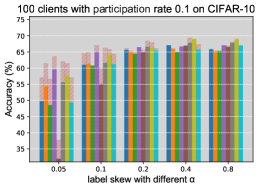
(a) Different label skews

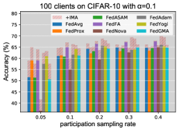
(b) Different participation rates

(c) Different local epochs

Figure 6: Performance of all methods with and without IMA on different federated setups.

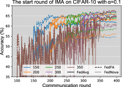
(a) Different start round

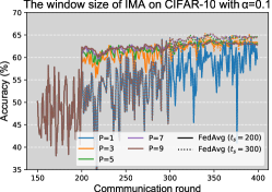
(b) Different window size

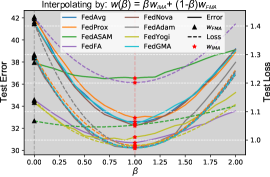
(c) Test error/loss landscape

Figure 7: Ablation studies on IMA and landscape visualization between FMA and IMA models.

7.3 Ablation Study on IMA

7.3.1 Ablation on Starting Rounds and Window Size of IMA

The results in Table II indicate that starting IMA at a later round requires higher communication overhead. However, Figure 7(a) shows that starting IMA at the $350$th round leads to the best final performance in terms of accuracy compared with other methods. This finding demonstrates a trade-off between communication efficiency and performance in IMA. Moreover, increasing the window size improves the training stability but can hurt the final accuracy if IMA starts early. This can be observed in the case of FedAvg with $t_{s}=200$ and $P=9$, where a lower accuracy is achieved compared with other cases in Figure 7(b)).

Table III: Accuracy v.s. decay schemes.

IMA w/ decay	Exp Decay	Const LR	Cyclic Decay	Epoch Decay	NA Decay
FedAvg	64.57	64.50	64.27	62.96	63.96
FedProx	64.80	64.73	64.59	63.14	64.12
FedASAM	59.10	58.14	59.33	57.48	58.95
FedFA	67.03	66.62	66.94	66.63	66.40
FedNova	60.09	59.86	59.38	59.04	58.90
FedAdam	66.25	65.89	66.06	64.00	65.62
FedYogi	65.86	65.53	65.51	63.13	65.12
FedGMA	64.36	64.41	64.12	62.97	63.75

7.3.2 Ablation on Mild Client Exploration in IMA

As mentioned in Section 6, we adopt a more aggressive exponential lr decay per round in IMA than in FMA to restrict client exploration. To evaluate this design choice, we conduct experiments on CIFAR-10 with $\alpha=0.1$ to ablate IMA with different decay schemes, including a small constant lr (i.e., lr is $5\times 10^{-5}$ in IMA), cyclic lr decay [20] (i.e., decaying lr from $1\times 10^{-2}$ to $5\times 10^{-5}$ every 20 rounds), epoch decay [65] (i.e., decaying one local epoch per 20 rounds) and non-additional decay (NA). As shown in Table III, more aggressive decay schemes that sufficiently constrain client updates (e.g., exponential lr decay or small constant lr) outperform milder schemes. For instance, exponential decay achieves $64.57\%$ on FedAvg, compared with $62.96\%$ of epoch decay.

7.3.3 Test Loss Landscape between FMA and IMA Models

Figure 7(c) depicts the interpolation model between FMA and IMA models (both from the final round) to visualize the landscape of test error and test loss. The figure shows that the IMA models reach almost the center (i.e., the lowest point) of the test error and loss basins for all baselines, effectively alleviating the deviation mentioned in Section 6. In contrast, the FMA models only reach the basin’s wall, which verifies the deviation observed in Section 4. Moreover, Figure 7(c) shows that these methods reach various basins with different curvature. However, it does not necessarily hold that a flatter basin corresponds to lower error. For example, while FedASAM reaches the basin with the flattest curvature, it achieves the highest test error.

8 Discussions and Future works

This work advanced the understanding of how FMA operates in the presence of heterogeneous data and proposed employing IMA to enhance its performance. Firstly, we investigated the dynamics of the loss landscape of FMA during training and observed that client models closely surround the global model within the same basin. By employing test loss decomposition, we illustrated the relationship between the global model and client models, demonstrating that the client models’ heterogeneous bias and locality dominate the global model’s error after the early training stage. These findings motivated us to adopt IMA on global models in the late training stage rather than disregarding them in FMA. Our experiments showed that IMA significantly improves existing FL methods’ accuracy and communication efficiency under both label and feature skews.

Although we demonstrate the error relationship between the global model and client models based on expected loss decomposition in Section 5, explicitly quantifying this relationship in general cases remains necessary. Future works should analyze how each of the five factors dominates the error throughout the training process. In addition, an IMA variant with an adaptive starting round demonstrates the promising results in Table II and deserves investigation to reduce communication overhead without compromising generalization. Moreover, employing more flexible regularization between the global model and client models (e.g., elastic weight consolidation [54]) can further reduce the bias and locality in Theorem 1. We hope our study can serve as a valuable reference for further analysis and improvement of FL methods.

Tailin Zhou (Graduate student member, IEEE) received his B.Eng. degree in Electrical Engineering and Automation Engineering from Sichuan University in 2018, and his Master’s degree in Electrical Engineering from South China University of Technology in 2021. He is pursuing a Ph.D. degree at the Hong Kong University of Science and Technology under the supervision of Professor Jun Zhang and Professor Danny H.K. Tsang. His research interests include federated learning and its application in Internet of Things.

Zehong Lin (Member, IEEE) received the B.Eng. degree in information engineering from South China University of Technology in 2017, and the Ph.D. degree in information engineering from The Chinese University of Hong Kong in 2022. Since 2022, he has been with the Department of Electronic and Computer Engineering, The Hong Kong University of Science and Technology, where he is currently a Research Assistant Professor. His research interests include federated learning and edge AI.

Jun Zhang (Fellow, IEEE) received the B.Eng. degree in electronic engineering from the University of Science and Technology of China in 2004, the M.Phil. degree in information engineering from The Chinese University of Hong Kong in 2006, and the Ph.D. degree in Electrical and Computer Engineering from the University of Texas at Austin in 2009. He is an Associate Professor in the Department of Electronic and Computer Engineering at the Hong Kong University of Science and Technology. He is an IEEE Fellow. His research interests include cooperative AI and edge AI.

Danny H.K. Tsang (Life Fellow, IEEE) received the Ph.D. degree in electrical engineering from the Moore School of Electrical Engineering, University of Pennsylvania, Philadelphia, PA, USA, in 1989. After graduation, he joined the Department of Computer Science, Dalhousie University, Halifax, NS, Canada. He later joined the Department of Electronic and Computer Engineering, The Hong Kong University of Science and Technology (HKUST), Hong Kong, in 1992, where he is currently a Professor. He has also been serving as the Thrust Head of the Internet of Things Thrust, HKUST (Guangzhou), Guangzhou, China, since 2020. During his leave from HKUST from 2000 to 2001, he assumed the role of Principal Architect with Sycamore Networks, Chelmsford, MA, USA. His current research interests include cloud computing, edge computing, NOMA networks, and smart grids. He was a Guest Editor of the IEEE JOURNAL ON SELECTED AREAS IN COMMUNICATIONS’ special issue on Advances in P2P Streaming Systems, an Associate Editor of Journal of Optical Networking published by the Optical Society of America, and a Guest Editor of IEEE SYSTEMS JOURNAL. He currently serves as a member of the Special Editorial Cases Team of IEEE Communications Magazine. He was responsible for the network architecture design of Ethernet MAN/WAN over SONET/DWDM networks. He invented the 64B/65B encoding (U.S. Patent No.: U.S. 6 952 405 B2) and contributed it to the proposal for Transparent GFP in the T1X1.5 standard that was advanced to become the ITU G.GFP standard. The coding scheme has now been adopted by International Telecommunication Union (ITU)’s Generic Framing Procedure Recommendation GFP-T (ITUT G.7041/Y.1303) and Interfaces of the Optical Transport Network (ITU-T G.709). He has been elevated to an IEEE Fellow in 2012 and an HKIE Fellow in 2013. His current research interests include next-generation Internet, mobile edge computing and smart grids.

Appendix A: Proof

Proof of Lemma 1

Suppose clients do not have an extremely imbalanced dataset (i.e., $n_{i}/n_{j}\neq\infty$ when $i\neq j$).

Proof.

(Proof of Lemma 1) For client $k$ and the FMA’s model, we have:

$$\begin{aligned} f_{\mathbf{w}_{k}}(x)=f_{\mathbf{w}_{\rm FMA}}(x)+\langle\Delta f_{\mathbf{w}_{\rm FMA}}(x),\Delta_{k}\rangle+O(\|\Delta_{k}\|^{2})\end{aligned},$$ (6)

where $\langle\cdot,\cdot\rangle$ is the dot product, and $\Delta_{k}=\mathbf{w}_{k}-\mathbf{w}_{\rm FMA}$. Thus, we establish the relationship between the FMA-model function and the WENS function as:

$$f_{\rm WENS}(x)=\sum_{k=1}^{K}\frac{n_{k}}{n}f_{\mathbf{w}_{k}}(x)$$ (7)

$$= f_{\mathbf{w}_{\rm FMA}}(x)+\sum_{k=1}^{K}\frac{n_{k}}{n}\langle\Delta f_{\mathbf{w}_{\rm FMA}}(x),\Delta_{k}\rangle+\sum_{k=1}^{K}\frac{n_{k}}{n}O(\|\Delta_{k}\|^{2})$$

$$= f_{\mathbf{w}_{\rm FMA}}(x)+\langle\Delta f_{\mathbf{w}_{\rm FMA}}(x),\sum_{k=1}^{K}\frac{n_{k}}{n}\Delta_{k}\rangle+O(\|\Delta\|^{2})$$

$$= f_{\mathbf{w}_{\rm FMA}}(x)+O(\|\Delta\|^{2}),$$

where $\|\Delta\|=\max_{k}^{K}\|\Delta_{k}\|$, $n=\sum_{k}n_{k}$ is the total sample number. ∎

Proof of Theorem 1

Proof.

(Proof of Theorem 1) Substituting $f_{\rm WENS}(x)=\sum_{k=1}^{K}\frac{n_{k}}{n}f_{\mathbf{w}_{k}}$ into (2), we have:

$$\mathbb{E}_{\mathbf{\{w}_{k}\}_{k=1}^{K}\in\prod_{k}^{K}\mathcal{W}_{\mathcal{D}_{k}}}\mathcal{L}({\mathbf{\{w}_{k}\}_{k=1}^{K}})$$ (8)

$$= \mathbb{E}_{(x,y)\in\mathcal{D}}[({\rm{Bias}}\{f_{\rm WENS}|(x,y)\})^{2}+{\rm{Var}}\{f_{\rm WENS}|x\}].$$

For the bias term, we have:

$${\rm{Bias}}\{f_{\rm WENS}|(x,y)\}=y-\mathbb{E}_{\mathbf{\{w}_{k}\}_{k=1}^{K}}f_{\rm WENS}(x)$$ (9)

$$= y-\mathbb{E}_{\mathbf{\{w}_{k}\}_{k=1}^{K}}[\sum_{k=1}^{K}\frac{n_{k}}{n}f_{\mathbf{w}_{k}}(x)]$$

$$= y-\sum_{k=1}^{K}\frac{n_{k}}{n}\mathbb{E}_{\mathbf{w_{k}}}[f_{\mathbf{w}_{k}}(x)]$$

$$= \sum_{k=1}^{K}\frac{n_{k}}{n}(y-\mathbb{E}_{\mathbf{w_{k}}}[f_{\mathbf{w}_{k}}(x)]).$$

Taking the expectation of the bias term with respect to the global dataset, we have:

$$\mathbb{E}_{(x,y)\in\mathcal{D}}({\rm{Bias}}\{f_{\rm WENS}|(x,y)\})^{2}$$ (10)

$$= \frac{1}{n}\sum_{(x,y)\in\mathcal{D}}[\sum_{k=1}^{K}\frac{n_{k}}{n}\underbrace{\mathbb{I}[{(x,y)\in\mathcal{D}_{k}}](y-\mathbb{E}_{\mathbf{w_{k}}}[f_{\mathbf{w}_{k}}(x)])}_{{\rm{TrainBias}}\{f_{\mathbf{w}_{k}}|(x,y)\}}$$

$$+\sum_{k=1}^{K}\frac{n_{k}}{n}\underbrace{\mathbb{I}[{(x,y)\in\mathcal{D}\setminus\mathcal{D}_{k}}](y-\mathbb{E}_{\mathbf{w_{k}}}[f_{\mathbf{w}_{k}}(x)])}_{{\rm{HeterBias}}\{f_{\mathbf{w}_{k}}|(x,y)\}}]^{2}.$$

For the variance term, we have:

$${\rm{Var}}\{f_{\rm WENS}|(x,y)\}$$ (11)

$$= \mathbb{E}_{\mathbf{\{w}_{k}\}_{k=1}^{K}}[(\sum_{k=1}^{K}\frac{n_{k}}{n}f_{\mathbf{w}_{k}}(x)-\mathbb{E}_{\mathbf{\{w}_{k}\}_{k=1}^{K}}[\sum_{k=1}^{K}\frac{n_{k}}{n}f_{\mathbf{w}_{k}}(x)])^{2}]$$

$$= \sum_{k=1}^{K}\frac{n_{k}^{2}}{n^{2}}\underbrace{\mathbb{E}_{\mathbf{{w}_{k}}}[(f_{\mathbf{w}_{k}}(x)-\mathbb{E}_{\mathbf{{w}_{k}}}[f_{\mathbf{w}_{k}}(x)])^{2}]}_{{\rm Var}\{f_{\mathbf{w}_{k}}|x\}}$$

$$+\sum_{k}\sum_{k\neq{k^{\prime}}}\frac{n_{k}n_{{k^{\prime}}}}{n^{2}}{{\rm Cov}\{f_{\mathbf{w}_{k},\mathbf{w}_{{k^{\prime}}}}|x\}},$$

where ${\rm Cov}\{f_{\mathbf{w}_{k},\mathbf{w}_{{k^{\prime}}}}|x\}=\mathbb{E}_{\mathbf{{w}_{k}},\mathbf{{w}_{{k^{\prime}}}}}[(f_{\mathbf{w}_{k}}(x)-\mathbb{E}_{\mathbf{{w}_{k}}}[f_{\mathbf{w}_{k}}(x)])$ $(f_{\mathbf{w}_{{k^{\prime}}}}(x)-\mathbb{E}_{\mathbf{{w}_{{k^{\prime}}}}}[f_{\mathbf{w}_{{k^{\prime}}}}(x)])]$. Taking the expectation of the variance term with respect to the global dataset, we have:

$$\mathbb{E}_{(x,y)\in\mathcal{D}}({\rm{Var}}\{f_{\rm ENS}|(x,y)\})$$ (12)

$$= \mathbb{E}_{(x,y)\in\mathcal{D}}({\sum_{k=1}^{K}\frac{n_{k}^{2}}{n^{2}}{\rm Var}\{f_{\mathbf{w}_{k}}|x\}}$$

$$+{\sum_{k}\sum_{{k^{\prime}}}\frac{n_{k}n_{{k^{\prime}}}}{n^{2}}{\rm Cov}\{f_{\mathbf{w}_{k},\mathbf{w}_{k^{\prime}}}|x\}})$$

$$= \frac{1}{n}\sum_{(x,y)\in\mathcal{D}}{\sum_{k=1}^{K}\frac{n_{k}^{2}}{n^{2}}{\rm Var}\{f_{\mathbf{w}_{k}}|x\}}$$

$$+\frac{1}{n}\sum_{(x,y)\in\mathcal{D}}{\sum_{k}\sum_{{k^{\prime}}}\frac{n_{k}n_{{k^{\prime}}}}{n^{2}}{\rm Cov}\{f_{\mathbf{w}_{k},\mathbf{w}_{k^{\prime}}}|x\}}.$$

Using the Taylor expansion at the zeroth order of the loss, we extend Lemma 1 and obtain:

$$\mathcal{L}(\mathbf{{w}_{\rm FMA}})=\mathbb{E}_{(x,y)\in\mathcal{D}}[l(f_{\mathbf{{w}_{\rm FMA}}}(x);y)]$$ (13)

$$= \mathbb{E}_{(x,y)\in\mathcal{D}}[l(f_{\rm WENS}(x);y)]$$

$$+O(\|f_{\mathbf{{w}_{\rm FMA}}}(x)-f_{\rm WENS}(x)\|_{2})$$

$$= \mathcal{L}({\mathbf{\{w}_{k}\}_{k=1}^{K}})+O(\Delta^{2}).$$

Finally, combining (10) and (12) with (8), we have:

$$\mathbb{E}_{\mathbf{\{w}_{k}\}_{k=1}^{K}\in\prod_{k}^{K}\mathcal{W}_{\mathcal{D}_{k}}}\mathcal{L}(\mathbf{{w}_{\rm FMA}})$$ (14)

$$= \mathbb{E}_{\mathbf{\{w}_{k}\}_{k=1}^{K}\in\prod_{k}^{K}\mathcal{W}_{\mathcal{D}_{k}}}\mathcal{L}({\mathbf{\{w}_{k}\}_{k=1}^{K}})+O(\Delta^{2})$$

$$= \mathbb{E}_{(x,y)\in\mathcal{D}}[({\rm{Bias}}\{f_{\rm WENS}|(x,y)\})^{2}+{\rm{Var}}\{f_{\rm WENS}|x\}]+O(\Delta^{2})$$

$$= \frac{1}{n}\sum_{(x,y)\in\mathcal{D}}[\sum_{k=1}^{K}\frac{n_{k}}{n}{\rm{TrainBias}}\{f_{\mathbf{w}_{k}}|(x,y)\}$$

$$+\frac{n_{k}}{n}{\rm{HeterBias}}\{f_{\mathbf{w}_{k}}|(x,y)\}]^{2}$$

$$+{\sum_{k=1}^{K}\frac{n_{k}^{2}}{n^{2}}{\rm Var}\{f_{\mathbf{w}_{k}}|x\}}+{\sum_{k}\sum_{{k^{\prime}}}\frac{n_{k}n_{{k^{\prime}}}}{n^{2}}{\rm Cov}\{f_{\mathbf{w}_{k},\mathbf{w}_{k^{\prime}}}|x\}}$$

$$+O(\Delta^{2}).$$

∎

Appendix B: Loss Landscape Visualization

Loss Landscape Visualization of Cross-device and Cross-silo FL

We examine two common FL frameworks to demonstrate the similarity of loss landscapes across different FL frameworks: cross-device FL, and cross-silo FL [10]. The number of clients involved in cross-silo FL is small (e.g., the cross-silo FL shown in Figure 8 includes ten clients), and all clients participate fully in each communication round. On the other hand, cross-device FL requires a large number of clients, and only a subset of them participate in each round (e.g., the cross-device FL in Figure 8 involves 100 clients with 0.1 participation rate for each round). Figure 8 depicts the loss landscape visualization with three models on the global dataset for both cross-device and cross-silo FL settings.

Similar to the FMA’s geometric properties observed from Figure 1, the FMA model (i.e., the white cross) achieves lower test loss and error than the individual client models (i.e., the black triangles) throughout the training process in both settings. Furthermore, both FL settings illustrate that FMA maintains the client and global models closely located within a shared basin. Notably, the deviation between the white cross and the lowest point of the basin in terms of loss/error is smaller in cross-device FL than cross-silo FL, as shown in Figure 8. This finding supports the analysis presented in Section 6, which suggests that low participation rates exacerbate the deviation.

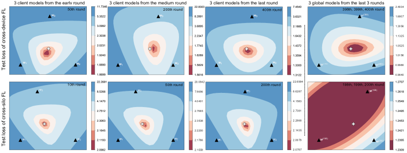
Figure 8: Loss landscape visualization with three models on global testset in cross-device and cross-silo FL.

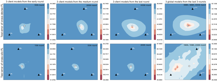
Figure 9: Error landscape visualization with three models on global testset in cross-device and cross-silo FL.

In addition to the loss landscape, we visualize the classification error landscape on the global dataset for both settings in Figure 9. The observed geometric properties of FMA in Figure 9 are similar to those depicted in Figure 8. Therefore, we omit the detailed descriptions here to avoid repetition.

Loss landscape visualization under Different Models, Datasets and Heterogeneous Data Settings

To further explore the geometric properties of FMA, we visualize the loss landscape of FL under various models (including the CNN model and the ResNet model), datasets (including FMNIST and CIFAR-10), and data heterogeneity (including label skews with $\#C=2$ and $\alpha=0.1$). The visualization results are presented in Figure 10. The geometric properties of FMA discussed in Section 4 are consistent with those observed in Figure 10. Regardless of the specific FL setup, FMA ensures that both client and global models reside within a common basin. This geometric insight sheds light on how FMA effectively prevents client models from over-fitting to their respective datasets (i.e., FMA mitigates the over-fitting information of client models being aggregated into the global model) and improves the generalization performance of the global model.

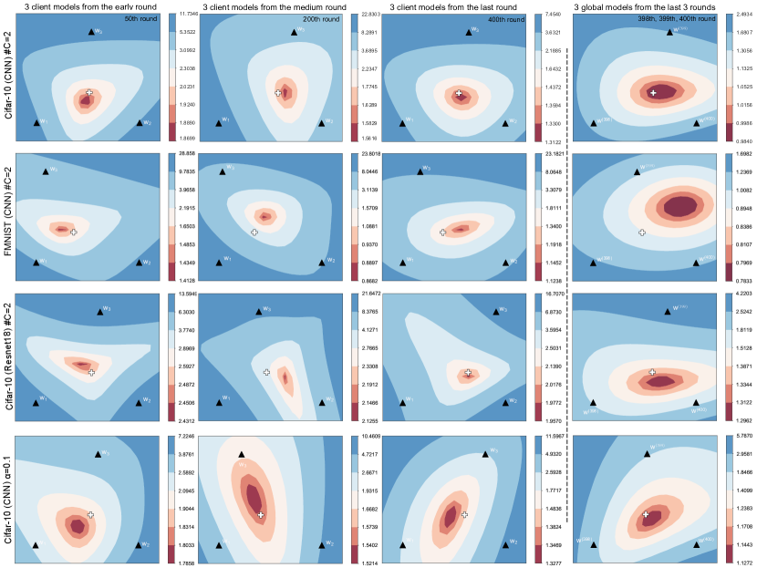
Figure 10: Loss landscape visualization of client and global models in FL under different setups: The first row illustrates the visualization of CNN models trained under data heterogeneity $\#C=2$ of CIFAR-10; The second row illustrates the visualization of CNN models trained under $\#C=2$ on FMNIST; The third row illustrates the visualization of Resnet18 trained under $\#C=2$ on CIFAR-10; The fourth row illustrates the visualization of CNN models trained with a Dirichlet parameter $\alpha=0.1$ on CIFAR-10.

Appendix C: Further Analysis

For the analysis of the variance term, we set $n_{i}=n_{j}$ (i.e., the number of client samples is the same) to isolate the impact of weighted averaging on the loss decomposition in Theorem 1. Consequently, we have the following corollary:

Corollary 2.

(Loss decomposition of FMA with the same client sample sizes. Extended from Theorem 1.) Given $K$ client models $\mathbf{\{w}_{k}\}_{k=1}^{K}\in\prod_{k}^{K}\mathcal{W}_{\mathcal{D}_{k}}$ and $n_{i}/n=n_{j}/n=1/K$, we can decompose the expected loss of the FMA’s model $\mathbf{w}_{\rm FMA}$ on $\mathcal{D}$ as:

$$\mathbb{E}_{\mathbf{\{w}_{k}\}_{k=1}^{K}}\mathcal{L}(\mathbf{{w}_{\rm FMA}})=\frac{1}{nK^{2}}\sum_{(x,y)\in\mathcal{D}}[\sum_{k=1}^{K}{\rm{TrainBias}}\{f_{\mathbf{w}_{k}}|(x,y)\}$$ (15)

$$+{\rm{HeterBias}}\{f_{\mathbf{w}_{k}}|(x,y)\}]^{2}+\frac{1}{K}\underbrace{\sum_{k=1}^{K}\frac{1}{K}{\rm Var}\{f_{\mathbf{w}_{k}}|x\}}_{\overline{\rm Var}\{f_{\mathbf{\{w}_{k}\}_{k=1}^{K}}|x\}}$$

$$+\sum_{k}\frac{K-1}{K^{2}}\underbrace{\sum_{{k^{\prime}}\neq k}\frac{1}{K-1}{\rm Cov}\{f_{\mathbf{w}_{k},\mathbf{w}_{k^{\prime}}}|x\}}_{\overline{\rm Cov}\{f_{\mathbf{{w}_{k}},\mathbf{{w}_{k^{\prime}}}}|x\}}+O(\Delta^{2}),$$

where ${\rm Var}\{f_{\mathbf{w}_{k}}|x\}=\mathbb{E}_{\mathbf{{w}_{k}}}[(f_{\mathbf{w}_{k}}(x)-\mathbb{E}_{\mathbf{{w}_{k}}}[f_{\mathbf{w}_{k}}(x)])^{2}]$; ${\rm Cov}\{f_{\mathbf{w}_{k},\mathbf{w}_{k^{\prime}}}|x\}=\mathbb{E}_{\mathbf{{w}_{k}},\mathbf{{w}_{{k^{\prime}}}}}[(f_{\mathbf{w}_{k}}(x)-\mathbb{E}_{\mathbf{{w}_{k}}}[f_{\mathbf{w}_{k}}(x)])$$(f_{\mathbf{w}_{{k^{\prime}}}}(x)$ $-\mathbb{E}_{\mathbf{{w}_{{k^{\prime}}}}}[f_{\mathbf{w}_{{k^{\prime}}}}(x)])]$; $\overline{\rm Var}\{f_{\mathbf{\{w}_{k}\}_{k=1}^{K}}|x\}$ denotes the mean prediction variance of client models when given a sample $(x,y)\in\mathcal{D}$; $\overline{\rm Cov}\{f_{\mathbf{{w}_{k}},\mathbf{{w}_{k^{\prime}}}}|x\}$ denotes the mean prediction covariance between two client models when given a sample $(x,y)\in\mathcal{D}$.

With Corollary 2, the covariance term and the sum of the variance term (i.e., ${\rm Var}\{f_{\mathbf{w}_{k}}|x\}={\rm Cov}\{f_{\mathbf{w}_{k},\mathbf{w}_{k^{\prime}}}|x\}$ when client models are identically distributed (i.e., client models are trained on homogeneous datasets with the same training configurations). In this case, the effect of the variance and covariance factors in Theorem 1 is equal to a single client model, rendering the aggregation of more client models in FMA useless.

Appendix D: Experiment Settings

Models

Table IV outlines the models used in all the experiments, including validation, test, and ablation experiments. To isolate the controversial effect of BN layers on FL, we follow [62] to replace the BN layer with the GroupNorm layer in all experiments. Our models adhere to the architectures reported in the respective baseline works for a fair comparison. Specifically, for the experiments conducted on the FMNIST and CIFAR-10 datasets, we employ a CNN model consisting of two 5x5 convolutional layers followed by 2x2 max pooling and two fully connected layers with ReLU activation. This architecture aligns with the model used in [26]. For the CIFAR-10/100 experiments, we adopt the ResNet-18 architecture [59] with a linear projector. This choice is consistent with the models employed in [29] and [57]. Lastly, for the Digit Fives dataset, we employ a CNN model with three 5x5 convolutional layers followed by five GroupNorm layers.

Baseline Settings

Table V provides the additional hyper-parameters specific to different baselines. These hyper-parameters are chosen based on the setups reported in the respective baseline works. Here is a brief description of the role of hyper-parameters in each baseline:

• FedProx and FedFA: These baselines modify the loss function by adding a proximal term at the client side. The best coefficient of the proximal term is selected from the given range [0.1, 0.01, 0.001]. This coefficient controls the trade-off between the proximal and main loss functions.

• FedASAM: This baseline utilizes the SAM technique as the client loss function. The hyper-parameters $\eta_{\rm SAM}$ and $\rho_{\rm SAM}$ control the noise introduced in SAM, affecting the exploration-exploitation trade-off during optimization.

• FedAdam and FedYogi: These baselines apply adaptive momentum to the global update on the server side. The hyper-parameters include the server learning rate (lr) $\eta$, decay parameters $\beta_{1}$, $\beta_{2}$, and the degree of adaptivity $\tau_{1}$. These hyper-parameters control the adaptation of the server-side optimizer’s momentum over time.

• FedGMA: This baseline employs the AND-Masked gradient update based on the masking threshold $\epsilon$. The masking threshold determines the level of sparsity in the gradient updates and improves the flatness of the global model.

It is worth noting that FedAvg and FedNova do not require additional hyper-parameters beyond the standard optimization parameters.

Table IV: Parameter settings for all the models used in our experiments. Group normalization layers split input channels into two groups in all models.

	Dataset
	FMNIST	CIFAR-10/100			Digit Five	PACS
Layer	CNN	CNN	VGG11	Resnet18	CNN	AlexNet
1	Conv2d(1,32,5) ReLU,MaxPool2D(2,2)	Conv2d(3,64,5) ReLU,MaxPool2D(2,2)	Basicbone of VGG11 with GN	Basicbone of Resnet18 with GN	Conv2d(3,64,5,1,2) GN(2,64) ReLU,MaxPool2D(2,2)	Basicbone of AlexNet with GN
2	Conv2d(1,32,5) ReLU,MaxPool2D(2,2)	Conv2d(64,64,5) ReLU,MaxPool2D(2,2)	VGG11.FC(512,128)	Resnet18.FC(512,128)	Conv2d(64,64,5,1,2) GN(2,64) ReLU,MaxPool2D(2,2)	Resnet18.FC(4096,512)
3	FC(512,384) ReLU	FC(1600,384) ReLU	FC(128,10)	FC(128,10)	Conv2d(64,128,5,1,2) GN(2,128) ReLU,MaxPool2D(2,2)	FC(512,10)
4	FC(384,128)	FC(384,128)			FC(6272, 2048) ReLU
5	FC(128,10)	FC(128,10)			FC(2048,128)
6					FC(128,10)

Table V: Hyper-parameter setups for all the baselines. FedAvg and FedNova are not involved as they do not require additional hyper-parameters.

Hyper- parameter	FedProx (+IMA)	FedASAM (+IMA)	FedFA (+IMA)	FedAdam (+IMA)	FedYogi (+IMA)	FedGMA (+IMA)
	coefficient of proximal term: Best from [0.1, 0.01,0.001]	CNN models: $\rho_{\rm SAM}$=0.7, $\eta_{\rm SAM}$=0.2	coefficient of proximal term: Best from [0.1, 0.01,0.001]	$\eta$ = 0.01		$\eta=0.0001$
		Other models: $\rho_{\rm SAM}$=0.2, $\eta_{\rm SAM}$=0.05	coefficient of anchor updates: 0.9	$\beta_{1}$ = 0.9		$\epsilon=0.8$
				$\beta_{2}$ = 0.99
				$\tau_{1}$ = 0.001
Refer	-	Authors’ codes	Appendix in [26]: the same experiments	Benchmark:Flower		Reproduces codes

Settings of Visualization and Validation experiments

Table VI provides the specific setups for all visualization and validation experiments. The experiments are performed using PyTorch on a single node of the High-Performance Computing platform. The node is equipped with 4 NVIDIA A30 Tensor Core GPUs, each with 24GB of memory. The setups include various parameters and configurations specific to each experiment, such as the model architecture, dataset, number of clients, batch size, learning rate, optimizer, and other relevant details.

Table VI: Setup of all visualization and validation experiments in this work. $\#C=2$ implies that each client holds two class shards of the training dataset, each containing 250 samples. $\alpha=0.1$ represents to split training dataset with Dirichlet distribution $Dir(\alpha)=0.1$ as in [56].

	FL	client number	client sampling	local epoch	local batch	lr (momentum)	lr decay per round	round	dataset	heterogeneious data(C:class)	model
Figure 1, 9	Cross-device FL	100	0.1	5	50	0.01(0.9)	0	400	CIFAR-10	$\#C=2$	CNN
Figure 8, 9	Cross-silo FL	10	1	5	50	0.01(0.9)	0	200	CIFAR-10	$\#C=2$	CNN
Figure 10	Cross-device FL	100	0.1	5	50	0.01(0.9)	0	400	CIFAR-10	$\#C=2$,$\alpha=0.1$	CNN, Resnet18
Figure 2, 3,4	Cross-silo FL	10	1	5	50	0.01(0.9)	0/0.01	400	CIFAR-10	$\#C=2$	CNN
Figure 5	Cross-device FL	100	0.1	5	50	0.01(0.9)	0	400	CIFAR-10	$\#C=2$	CNN

Settings of Test Experiments

Table VII provides the setup details for all test experiments conducted in this work. The table includes information such as the client number, participation rate, local epoch number, lr, decay scheme, total communication rounds, model, and specific setups of IMA. Please refer to Table VII for a comprehensive overview of the experimental configurations.

Table VII: Setup of all test experiments in Table I.

Table I	client number	participation rate	local epoch	local batch	lr (momentum)	lr decay per round	round	windows size	IMA lr decay	start IMA(0.75)	model
FMNIST	100	0.1	5	50	0.01(0.9)	0.01	300	5	0.03	225	CNN
CIFAR-10	100	0.1	5	50	0.01(0.9)	0.01	400	5	0.03	300	CNN,Resnet18
CIFAR-100	100	0.1	5	50	0.01(0.9)	0.01	300,400	5	0.03	225,300	VGG11,Resnet18
Digit Five	100	0.1	5	50	0.01(0.9)	0.01	200	5	0.03	150	CNN w/ GN
PACS	80	0.2	5	50	0.01(0.9)	0.01	400	5	0.03	300	AlexNet w/ GN

References

- [1] B. McMahan, E. Moore, D. Ramage, S. Hampson, and B. A. y Arcas, “Communication-efficient learning of deep networks from decentralized data,” in Proc. Int. Conf. Artif. Intell. Statist. (AISTATS), Ft. Lauderdale, FL, USA, Apr. 2017, pp. 1273–1282.
- [2] Y. Zhao, M. Li, L. Lai, N. Suda, D. Civin, and V. Chandra, “Federated learning with non-iid data,” [Online]. Available https://arxiv.org/pdf/1806.00582.pdf.
- [3] Q. Wu, X. Chen, Z. Zhou, and J. Zhang, “Fedhome: Cloud-edge based personalized federated learning for in-home health monitoring,” IEEE Trans. Mobile Comput., vol. 21, no. 8, pp. 2818–2832, Aug. 2020.
- [4] W. Zhang, D. Yang, W. Wu, H. Peng, N. Zhang, H. Zhang, and X. Shen, “Optimizing federated learning in distributed industrial iot: A multi-agent approach,” IEEE J. Sel. Areas Commun., vol. 39, no. 12, pp. 3688–3703, Oct. 2021.
- [5] M. Chen, Z. Yang, W. Saad, C. Yin, H. V. Poor, and S. Cui, “A joint learning and communications framework for federated learning over wireless networks,” IEEE Trans. Wirel. Commun., vol. 20, no. 1, pp. 269–283, Oct. 2020.
- [6] S. Wang, M. Chen, C. G. Brinton, C. Yin, W. Saad, and S. Cui, “Performance optimization for variable bitwidth federated learning in wireless networks,” IEEE Trans. Wirel. Commun., Mar. 2023.
- [7] M. N. Nguyen, N. H. Tran, Y. K. Tun, Z. Han, and C. S. Hong, “Toward multiple federated learning services resource sharing in mobile edge networks,” IEEE Trans. Mobile Comput., vol. 22, no. 1, pp. 541–555, Jun. 2021.
- [8] Z. Feng, X. Chen, Q. Wu, W. Wu, X. Zhang, and Q. Huang, “Feddd: Toward communication-efficient federated learning with differential parameter dropout,” IEEE Trans. Mobile Comput., no. 01, pp. 1–18, Aug. 2023.
- [9] X. Zhang, Z. Chang, T. Hu, W. Chen, X. Zhang, and G. Min, “Vehicle selection and resource allocation for federated learning-assisted vehicular network,” IEEE Trans. Mobile Comput., pp. 1–12, Jun. 2023.
- [10] P. Kairouz, H. B. McMahan, B. Avent, A. Bellet, M. Bennis, A. N. Bhagoji, K. Bonawitz, Z. Charles, G. Cormode, R. Cummings et al., “Advances and open problems in federated learning,” Found. Trends Mach. Learn., vol. 14, no. 1–2, pp. 1–210, 2021.
- [11] J. Wang, Z. Charles, Z. Xu, G. Joshi, H. B. McMahan, M. Al-Shedivat, G. Andrew, S. Avestimehr, K. Daly, D. Data et al., “A field guide to federated optimization,” [Online]. Available https://arxiv.org/pdf/2107.06917.pdf.
- [12] B. T. Polyak and A. B. Juditsky, “Acceleration of stochastic approximation by averaging,” SIAM J. Control Optim., vol. 30, no. 4, pp. 838–855, 1992.
- [13] X. Lian, C. Zhang, H. Zhang, C.-J. Hsieh, W. Zhang, and J. Liu, “Can decentralized algorithms outperform centralized algorithms? a case study for decentralized parallel stochastic gradient descent,” in Proc. Conf. Adv. Neural Inf. Process. Syst. (NeurIPS), Long Beach, CA, USA, Dec. 2017, pp. 5330–5340.
- [14] J. Zhang, C. De Sa, I. Mitliagkas, and C. Ré, “Parallel sgd: When does averaging help?” [Online]. Available https://arxiv.org/pdf/1606.07365.pdf.
- [15] A. Koloskova, N. Loizou, S. Boreiri, M. Jaggi, and S. Stich, “A unified theory of decentralized sgd with changing topology and local updates,” in Proc. Int. Conf. Mach. Learn. (ICML), Virtual Event, Jul. 2020, pp. 5381–5393.
- [16] X. Li, K. Huang, W. Yang, S. Wang, and Z. Zhang, “On the convergence of fedavg on non-iid data,” in Proc. Int. Conf. Learn. Repr. (ICLR), Addis Ababa, Ethiopia, Apr. 2020.
- [17] H. Yu, S. Yang, and S. Zhu, “Parallel restarted sgd with faster convergence and less communication: Demystifying why model averaging works for deep learning,” in Proc. AAAI Conf. Artif. Intell. (AAAI), vol. 33, Honolulu, Hawaii, USA,, Jan. 2019, pp. 5693–5700.
- [18] J. Wang, R. Das, G. Joshi, S. Kale, Z. Xu, and T. Zhang, “On the unreasonable effectiveness of federated averaging with heterogeneous data,” [Online]. Available https://arxiv.org/pdf/2206.04723.pdf.
- [19] P. Jain, S. Kakade, R. Kidambi, P. Netrapalli, and A. Sidford, “Parallelizing stochastic gradient descent for least squares regression: mini-batching, averaging, and model misspecification,” J. Mach. Learn. Res., vol. 18, pp. 223:1–223:42, Jul. 2017.
- [20] P. Izmailov, D. Podoprikhin, T. Garipov, D. Vetrov, and A. G. Wilson, “Averaging weights leads to wider optima and better generalization,” in Proc. Int. Conf. on Uncert. in Artif. Intell. (UAI), Monterey, California, USA, Aug., pp. 876–885.
- [21] V. Gupta, S. A. Serrano, and D. DeCoste, “Stochastic weight averaging in parallel: Large-batch training that generalizes well,” in Proc. Int. Conf. Learn. Repr. (ICLR), Addis Ababa, Ethiopia, Apr. 2020.
- [22] D. Caldarola, B. Caputo, and M. Ciccone, “Improving generalization in federated learning by seeking flat minima,” in Proc. Eur. Conf. Comp. Vision (ECCV), Tel Aviv, Israel, Oct. 2022, pp. 654–672.
- [23] S. Lee, S. Purushwalkam Shiva Prakash, M. Cogswell, V. Ranjan, D. Crandall, and D. Batra, “Stochastic multiple choice learning for training diverse deep ensembles,” in Proc. Conf. Adv. Neural Inf. Process. Syst. (NeurIPS), Barcelona, Spain, Dec. 2016, pp. 2119–2127.
- [24] A. Rame, M. Kirchmeyer, T. Rahier, A. Rakotomamonjy, P. Gallinari, and M. Cord, “Diverse weight averaging for out-of-distribution generalization,” in Proc. Conf. Adv. Neural Inf. Process. Syst. (NeurIPS), LA, CA, USA, May 2022.
- [25] T. Li, A. K. Sahu, M. Zaheer, M. Sanjabi, A. Talwalkar, and V. Smith, “Federated optimization in heterogeneous networks,” in Proc. Mach. Learn. Syst. (MLSys), Austin, TX, USA, Mar. 2020.
- [26] T. Zhou, J. Zhang, and D. Tsang, “Fedfa: Federated learning with feature anchors to align feature and classifier for heterogeneous data,” IEEE Trans. Mobile Comput., pp. 1–17, Oct. 2023.
- [27] Z. Li, Z. Lin, J. Shao, Y. Mao, and J. Zhang, “Fedcir: Client-invariant representation learning for federated non-iid features,” [Online]. Available https://arxiv.org/pdf/2308.15786.pdf.
- [28] J. Wang, Q. Liu, H. Liang, G. Joshi, and H. V. Poor, “Tackling the objective inconsistency problem in heterogeneous federated optimization,” in Proc. Conf. Adv. Neural Inf. Process. Syst. (NeurIPS), Virtual Event, Dec. 2020, pp. 7611–7623.
- [29] S. J. Reddi, Z. Charles, M. Zaheer, Z. Garrett, K. Rush, J. Konečný, S. Kumar, and H. B. McMahan, “Adaptive federated optimization,” in Proc. Int. Conf. Learn. Repr. (ICLR), Virtual Event, May 2021.
- [30] I. Tenison, S. A. Sreeramadas, V. Mugunthan, E. Oyallon, E. Belilovsky, and I. Rish, “Gradient masked averaging for federated learning,” [Online]. Available https://openreview.net/pdf?id=REAyrhRYAo.
- [31] Z. Li, J. Shao, Y. Mao, J. H. Wang, and J. Zhang, “Federated learning with gan-based data synthesis for non-iid clients,” in FL Workshop in Proc. Int. Joint Conf Artif. Intell (IJCAI), vol. 13448, Vienna, Austria, Jul. 2022, pp. 17–32.
- [32] Y. Sun, J. Shao, S. Li, Y. Mao, and J. Zhang, “Stochastic coded federated learning with convergence and privacy guarantees,” in IEEE Int. Symp. Inf. Theory (ISIT), Espoo, Finland, Aug. 2022, pp. 2028–2033.
- [33] J. Shao, Y. Sun, S. Li, and J. Zhang, “Dres-fl: Dropout-resilient secure federated learning for non-iid clients via secret data sharing,” in Proc. Conf. Adv. Neural Inf. Process. Syst. (NeurIPS), LA, CA, USA, May 2022.
- [34] S. P. Karimireddy, S. Kale, M. Mohri, S. Reddi, S. Stich, and A. T. Suresh, “Scaffold: Stochastic controlled averaging for federated learning,” in Proc. Int. Conf. Mach. Learn. (ICML), vol. 119, Virtual Event, 2020, pp. 5132–5143.
- [35] R. Sun, D. Li, S. Liang, T. Ding, and R. Srikant, “The global landscape of neural networks: An overview,” IEEE Signal Process. Mag., vol. 37, no. 5, pp. 95–108, Oct. 2020.
- [36] I. J. Goodfellow, O. Vinyals, and A. M. Saxe, “Qualitatively characterizing neural network optimization problems,” in Proc. Int. Conf. Learn. Repr. (ICLR), San Diego, CA, USA, May 2014.
- [37] H. Li, Z. Xu, G. Taylor, C. Studer, and T. Goldstein, “Visualizing the loss landscape of neural nets,” in Proc. Conf. Adv. Neural Inf. Process. Syst. (NeurIPS), vol. 31, Montreal, Canada, Dec 2018, pp. 6391–6401.
- [38] P. Foret, A. Kleiner, H. Mobahi, and B. Neyshabur, “Sharpness-aware minimization for efficiently improving generalization,” in Proc. Int. Conf. Learn. Repr. (ICLR), Virtual Event, May 2021.
- [39] J. Cha, S. Chun, K. Lee, H.-C. Cho, S. Park, Y. Lee, and S. Park, “Swad: Domain generalization by seeking flat minima,” in Proc. Conf. Adv. Neural Inf. Process. Syst. (NeurIPS), Virtual Event, Dec. 2021, pp. 22 405–22 418.
- [40] T. Garipov, P. Izmailov, D. Podoprikhin, D. P. Vetrov, and A. G. Wilson, “Loss surfaces, mode connectivity, and fast ensembling of dnns,” in Proc. Conf. Adv. Neural Inf. Process. Syst. (NeurIPS), vol. 31, Montreal, Canada, Dec., pp. 8803–8812.
- [41] F. Draxler, K. Veschgini, M. Salmhofer, and F. Hamprecht, “Essentially no barriers in neural network energy landscape,” in Proc. Int. Conf. Mach. Learn. (ICML), vol. 80, 10–15 Jul 2018, pp. 1309–1318.
- [42] Z. Li, H.-Y. Chen, H. W. Shen, and W.-L. Chao, “Understanding federated learning through loss landscape visualizations: A pilot study,” in Workshop on Federated Learning: Recent Advances and New Challenges (in Conjunction with NeurIPS 2022), 2022.
- [43] Z. Li, T. Lin, X. Shang, and C. Wu, “Revisiting weighted aggregation in federated learning with neural networks,” in Proc. Int. Conf. Mach. Learn. (ICML), Honolulu, Hawaii, USA, Jul. 2023, pp. 19 767–19 788.
- [44] S. Geman, E. Bienenstock, and R. Doursat, “Neural networks and the bias/variance dilemma,” Neural Comput., vol. 4, no. 1, pp. 1–58, Sep, 1992.
- [45] R. Kohavi, D. H. Wolpert et al., “Bias plus variance decomposition for zero-one loss functions,” in Proc. Int. Conf. Mach. Learn. (ICML), vol. 96, Bari, Italy, Jul. 1996, pp. 275–83.
- [46] P. Domingos, “A unified bias-variance decomposition,” in Proc. Int. Conf. Mach. Learn. (ICML), Austin, Texas, USA, Jul. 2000, pp. 231–238.
- [47] G. Brown, J. Wyatt, and P. Sun, “Between two extremes: Examining decompositions of the ensemble objective function,” in Multip. Classif. Syst.: 6th Int. Workshop, Seaside, CA, USA, Jun. 2005, pp. 296–305.
- [48] M. Belkin, D. Hsu, S. Ma, and S. Mandal, “Reconciling modern machine-learning practice and the classical bias–variance trade-off,” Proc. Natl. Acad. Sci. U.S.A., vol. 116, no. 32, pp. 15 849–15 854, Jul. 2019.
- [49] J. Shao, Z. Li, W. Sun, T. Zhou, Y. Sun, L. Liu, Z. Lin, and J. Zhang, “A survey of what to share in federated learning: Perspectives on model utility, privacy leakage, and communication efficiency,” [Online]. Available https://arxiv.org/pdf/2307.10655.pdf.
- [50] A. Krizhevsky, G. Hinton et al., “Learning multiple layers of features from tiny images,” [Online]. Available: https://www.cs.toronto.edu/~kriz/learning-features-2009-TR.pdf.
- [51] T. Zhou, J. Zhang, and D. H. Tsang, “Mode connectivity and data heterogeneity of federated learning,” [Online]. Available: https://arxiv.org/pdf/2309.16923.pdf.
- [52] N. Ye, K. Li, H. Bai, R. Yu, L. Hong, F. Zhou, Z. Li, and J. Zhu, “Ood-bench: Quantifying and understanding two dimensions of out-of-distribution generalization,” in Proc. IEEE/CVF Conf. Comput. Vision Pattern Recognit. (CVPR), New Orleans, LA, USA, Jun. 2022, pp. 7947–7958.
- [53] I. J. Goodfellow, M. Mirza, D. Xiao, A. Courville, and Y. Bengio, “An empirical investigation of catastrophic forgetting in gradient-based neural networks,” [Online]. Available: https://arxiv.org/pdf/1312.6211.pdf.
- [54] J. Kirkpatrick, R. Pascanu, N. Rabinowitz, J. Veness, G. Desjardins, A. A. Rusu, K. Milan, J. Quan, T. Ramalho, A. Grabska-Barwinska et al., “Overcoming catastrophic forgetting in neural networks,” Proc. Natl. Acad. Sci. U.S.A., vol. 114, no. 13, pp. 3521–3526, Mar. 2017.
- [55] H. Xiao, K. Rasul, and R. Vollgraf, “Fashion-mnist: a novel image dataset for benchmarking machine learning algorithms,” [Online]. Available: https://arxiv.org/pdf/1708.07747.pdf.
- [56] M. Yurochkin, M. Agarwal, S. Ghosh, K. Greenewald, N. Hoang, and Y. Khazaeni, “Bayesian nonparametric federated learning of neural networks,” in Proc. Int. Conf. Mach. Learn. (ICML), vol. 97, Long Beach, California, USA, Jun 2019, pp. 7252–7261.
- [57] X. Li, M. Jiang, X. Zhang, M. Kamp, and Q. Dou, “Fedbn: Federated learning on non-iid features via local batch normalization,” in Proc. Int. Conf. Learn. Repr. (ICLR), Virtual Event, May 2021.
- [58] D. Li, Y. Yang, Y.-Z. Song, and T. M. Hospedales, “Deeper, broader and artier domain generalization,” in Proc. IEEE/CVF Int. Conf. Comput. Vision (ICCV), Venice,Italy, Oct. 2017, pp. 5542–5550.
- [59] K. He, X. Zhang, S. Ren, and J. Sun, “Deep residual learning for image recognition,” in Proc. IEEE/CVF Conf. Comput. Vision Pattern Recognit. (CVPR), Las Vegas, NV, USA, Jun. 2016, pp. 770–778.
- [60] K. Simonyan and A. Zisserman, “Very deep convolutional networks for large-scale image recognition,” in Proc. Int. Conf. Learn. Repr. (ICLR), San Diego, CA, USA, May 2015.
- [61] A. Krizhevsky, I. Sutskever, and G. E. Hinton, “Imagenet classification with deep convolutional neural networks,” Commun. ACM, vol. 60, no. 6, pp. 84–90, Mar 2017.
- [62] K. Hsieh, A. Phanishayee, O. Mutlu, and P. Gibbons, “The non-iid data quagmire of decentralized machine learning,” in Proc. Int. Conf. Mach. Learn. (ICML), Virtual Event, Jul. 2020, pp. 4387–4398.
- [63] Q. Li, Y. Diao, Q. Chen, and B. He, “Federated learning on non-iid data silos: An experimental study,” in Proc. Int. Conf. Data Eng., (ICDE), Kuala Lumpur, Malaysia, May 2022, pp. 965–978.
- [64] W. Li and A. McCallum, “Pachinko allocation: Dag-structured mixture models of topic correlations,” in Proc. Int. Conf. Mach. Learn. (ICML), vol. 148, Pittsburgh, Pennsylvania, USA, Jun. 2006, pp. 577–584.
- [65] G. Pu, Y. Zhou, D. Wu, and X. Li, “Server averaging for federated learning,” [Online]. Available https://arxiv.org/pdf/2103.11619.pdf.