Control of wave scattering for robust coherent transmission in a disordered medium

Abstract

The spatial structure of the inhomogeneity in a disordered medium determines how waves scatter and propagate in it. We present a theoretical model of how the Fourier components of the disorder control wave scattering in a two-dimensional disordered medium, by analyzing the disordered Green’s function for scalar waves. By selecting a set of Fourier components with the appropriate wave vectors, we can enhance or suppress wave scattering to filter out unwanted waves and allow the robust coherent transmission of waves at specific angles and wavelengths through the disordered medium. Based on this principle, we propose an approach for creating selective transparency, band gaps and anisotropy in disordered media. This approach is validated by direct numerical simulations of coherent wave transmission over a wide range of incident angles and frequencies and can be experimentally realized in disordered photonic crystals. Our approach, which requires neither nontrivial topological wave properties nor a non-Hermitian medium, creates opportunities for exploring a broad range of wave phenomena in disordered systems.

I Introduction

Understanding how wave scattering in a disordered medium depends on the spatial structure of its inhomogeneity is important for progress in fundamental topics such as Anderson localization (Lagendijk et al., 2009; Modugno, 2010; Gredeskul et al., 2012; Segev et al., 2013; Mafi et al., 2019) and other transport phenomena (Sheng, 2006) as well as for a wide range of applications in photonics, (Wiersma, 2013; Yu et al., 2021) wave shaping, (Cao et al., 2022) imaging, (Bertolotti and Katz, 2022; Gigan, 2022) acoustics (Maynard, 2001), matter waves. (Billy et al., 2008) and even signal filtering. (Zangeneh-Nejad and Fleury, 2020) A remarkable insight into this relationship is found in Ref. (Kim and Heller, 2022) which shows how the electron wave interaction with the Berry potential can result in sharp Bragg-like scattering in spite of the absence of periodicity, with the outgoing waves distributed at specific angles in a manner akin to powder x-ray diffraction. Although this phenomenon is reported for electron waves in the Schroedinger equation, its underlying mechanism is not quantum mechanical and instead depends on the orientation of the incident wave vector $\bm{k}$ with respect to the Fourier (plane-wave or $\bm{q}$) components of the disorder, as represented by the Berry potential (Kim and Heller, 2022)

$$U(\bm{r};\{\phi_{j}\})=\frac{A}{\sqrt{N}}\sum_{j=1}^{N}\cos(\bm{p}_{j}\cdot\bm{r}+\phi_{j})\ ,$$ (1)

where $\bm{r}$ is the position vector in two dimensions, $A$ is a constant having the dimension of energy, $N$ is the number of Fourier components,  and $\bm{p}_{j}$ and $\phi_{j}$ denote the wave vector and phase of the $j$-th component, respectively, with $|\bm{p}_{j}|=q_{\text{c}}$.  The set of phases $\{\phi_{j}\}$ uniquely determines the spatial configuration of $U$, with each $\phi_{j}$ taking a value between $0$ and $2\pi$. Equation (1) describes a two-dimensional (2D) random potential constructed from a superposition of plane waves of equal wave number $q_{c}$ and distributed over all propagation angles. Because the Fourier components of the Berry potential are localized on a circular manifold of radius $q_{\text{c}}$, electron waves with $|\bm{k}|<q_{\text{c}}/2$ undergo minimal scattering and thus propagate without attenuation.

The finding suggests that the distribution of the Fourier components of the spatial disorder in a medium, as described by its reciprocal-space ($\bm{q}$) spectrum, has profound bearing for scattering and coherent wave transmission. This principle has been utilized in partially disordered media, (Yu et al., 2021; Vynck et al., ) in which the spatial distribution of particulate scatterers, characterized by the structure factor $S(\bm{q})$, can be correlated to generate transparency for a range of low-frequency waves. (Leseur et al., 2016) In stealthy hyperuniform (SH) systems in particular, (Torquato, 2018, 2016) where $S(\bm{q})=0$ for $0<|\bm{q}|\leq q_{\text{SH}}$ and $q_{\text{SH}}$ is the length scale of the absence of long-wavelength density fluctuations, this results in optical transparency for incident waves with wave numbers in the range of $|\bm{k}|<q_{\text{SH}}/2$, (Leseur et al., 2016) a finding closely related to that of Ref. (Kim and Heller, 2022). Indeed, one may interpret Eq. (1) as an analog of SH-type disorder for the Schroedinger equation, with the Berry potential behaving as a random scalar field with stealth hyperuniformity. (Torquato, 2016) Similar conditions for wave transparency in other SH systems have also been found by Kim and Torquato. (Kim and Torquato, 2020; Torquato and Kim, 2021)

A common conceptual thread that runs through the earlier articles on wave propagation in SH systems and Ref. (Kim and Heller, 2022) is that multiple wave scattering is suppressed when long-wavelength fluctuations are absent from the disorder configuration. In a classical disordered medium such as an inhomogeneous dielectric material with a position-dependent permittivity $\epsilon(\bm{r})$, (Frank and Lubatsch, 2011; Sheremet et al., 2020) the control of scattering is realized by modulating the Fourier components of $\epsilon(\bm{r})$ such that its reciprocal-space spectrum conforms to a particular distribution. Because multiple scattering underlies the wave transport phenomena of diffusion and Anderson localization, (Sheng, 2006) this control of scattering can potentially allow us to engineer the spectrum of waves transmitted through the disordered medium. We remark here that there is a slight difference between the complementary approaches of Ref. (Kim and Heller, 2022) and existing work on SH systems. (Torquato, 2018, 2016) The former proposes the reciprocal-space loci of the Fourier components of the disorder while the latter determines where the Fourier components should be excluded.

In our paper, we propose a systematic approach to engineer disorder for the selective suppression of scattering to allow the robust transmission of waves through the disordered medium for isotropic and selective transparency with orientation-dependent frequency-space windows. Although it is known that SH systems can act as isotropic low-pass filters, (Leseur et al., 2016; Torquato, 2018; Torquato and Kim, 2021) we go beyond the current state of the art through the introduction of a more elaborate substructure in the disorder spectrum, perhaps foreshadowed by the notion of directional hyperuniformity in Ref. (Torquato, 2016), and show, in the context of a scalar wave model, how disorder can be more precisely engineered to create mid-band gaps and orientation-dependent frequency-space transmission windows. We discuss its theoretical basis by analyzing how the Fourier-space distribution of the disorder affects wave scattering within the framework of the perturbative expansion of the disordered Green’s function and the incident wave function. A connection is also made with wave transparency in SH systems. Our analysis sheds light on the relationship between the disorder components and the on-shell scattering contributions to the disordered Green’s function, and predicts which plane waves are suppressed by disorder scattering. We use the insights from the analysis to discuss the conditions for isotropic and selective transparency. For validation, we compute the coherent transmission coefficient $t(\bm{k})$ (Anderson, 1985) for a wide range of incident angles and frequencies, using the Atomistic Green’s Function (AGF) method adapted from Refs. (Ong, 2018a, b), and obtain excellent agreement between the theory and simulation results. We demonstrate with an 2D example of how the disorder components can be combined to suppress wave scattering and to enable robust coherent transmission for certain plane-wave states at specific incident angles and frequencies. Possible experimental realizations are also suggested.

II Theory of disorder scattering of scalar waves

II.1 Scalar wave model

To discuss the scattering of a harmonic wave $\psi(\bm{r})$ of angular frequency $\omega$ at position $\bm{r}$ in a disordered medium, we use the Helmholtz wave equation

$$\left[\nabla^{2}+\left(\frac{\omega}{c}\right)^{2}\epsilon(\bm{r})\right]\psi(\bm{r})=0$$ (2)

where $\nabla^{2}$ and $c$ denote the 2D Laplace operator and wave speed, respectively. Equation (2) has been used to model transverse magnetic (TM) wave scattering in dielectric materials. (Davy et al., 2015; Froufe-Pérez et al., 2017; Brandstötter et al., 2019) For the purpose of this paper, we interpret the wave function $\psi(\bm{r})$ as the out-of-plane electric field component in a 2D dielectric medium (Davy et al., 2015; Froufe-Pérez et al., 2017; Brandstötter et al., 2019) although our results can be generalized to non-photonic systems. The static disorder is described by the permittivity function

$$\epsilon(\bm{r})=\epsilon_{0}[1+f(\bm{r})]\ ,$$

where $\epsilon_{0}=1$ denotes the permittivity of the disorder-free medium; $f(\bm{r})$, which denotes the disorder function corresponding to the position-dependent fluctuations of the permittivity, can be written as a sum of $N$ Fourier components like in Eq. (1), i.e.,

$$f(\bm{r})=\alpha\sqrt{\frac{2}{N}}\sum_{j=1}^{N}\cos(\bm{p}_{j}\cdot\bm{r}+\phi_{j})\ ,$$ (3)

with the normalization constraint $\lim_{\Omega\rightarrow\infty}\frac{1}{\Omega}\int_{\Omega}d\bm{r}|f(\bm{r})|^{2}=\alpha^{2}$ where $\Omega$ is the area of integration. The dimensionless constant $\alpha$ is the root-mean-square value of $f(\bm{r})$ and determines the relative disorder strength in Eq. (2) as well as the ‘coupling constant’ in the Dyson expansion which in our calculations, we set as $\alpha=0.1$. Instead of a discrete sum, Eq. (3) can also be expressed as an integral $f(\bm{r})=\alpha\int d\bm{q}\rho(\bm{q})\exp[i(\bm{q}\cdot\bm{r}+\phi_{\bm{q}})]$ where $\rho(\bm{q})$ is the ‘density of states’. The Fourier transform of $f(\bm{r})$ is given by $\mathcal{F}(\bm{q})=\frac{1}{h^{2}}\int_{\Omega}d\bm{r}e^{-i\bm{q}\cdot\bm{r}}f(\bm{r})=\alpha(\frac{2\pi}{h})^{2}\sum_{j=1}^{N}\sqrt{\frac{2}{N}}[e^{i\phi_{j}}\delta(\bm{q}-\bm{p}_{j})+e^{-i\phi_{j}}\delta(\bm{q}+\bm{p}_{j})]$ where $h$ is the 2D unit cell spacing. To facilitate our discussion of scattering, we rewrite Eq. (2) as (Frank and Lubatsch, 2011; Sheremet et al., 2020)

$$\left[\nabla^{2}+\kappa_{0}(\omega)^{2}+V(\omega,\bm{r})\right]\psi(\bm{r})=0\ ,$$ (4)

where $\kappa_{0}(\omega)=\omega\sqrt{\epsilon_{0}}/c$ is the frequency-dependent wave number for a plane-wave state in the disorder-free medium and $V(\omega,\bm{r})=\kappa_{0}(\omega)^{2}f(\bm{r})$ denotes the perturbation term which scales linearly with $\alpha$. In the absence of disorder where $V(\omega,\bm{r})=0$, Eq. (4) admits the plane-wave solution $\phi_{0}(\bm{r})=\frac{1}{\sqrt{\Omega}}e^{i\bm{k}\cdot\bm{r}}$ which describes a state with the wave vector $\bm{k}$, such that $|\bm{k}|=\kappa_{0}$.

II.2 Dyson expansion of the disordered Green’s function

To elucidate the relationship between wave scattering and disorder, we analyze the retarded Green’s function $G^{+}(\omega,\bm{r},\bm{r}^{\prime})$, which describes the $\omega$-dependent response at point $\bm{r}$ from a source at $\bm{r}^{\prime}$ in the disordered medium (Economou, 1983; Sheng, 2006) and is used in perturbative expansion of the wave function $\psi(\bm{r})$. Although some of the material in the following discussion on the Dyson expansion can be found in textbooks, we still discuss it in order to clarify the role of the Fourier components of $V(\omega,\bm{r})$ in scattering and wave transparency. Before we proceed, we give a qualitative bird’s eye view of our approach to determining wave transparency. In our analysis, we discuss how $V(\omega,\bm{r})$ affects the perturbative corrections to the Green’s function and the incoming plane-wave state, which are related through the Lippmann-Schwinger equation, and identify the condition for wave transparency under which these corrections vanish. For simplicity, we describe these corrections in terms of their Fourier transforms $\mathcal{V}(\bm{q})$ with respect to the reciprocal-space coordinates $\bm{k}$ and $\bm{q}$. This sheds light on the role of $\mathcal{V}(\bm{q})$ in the integrals for the perturbative corrections. We exploit the chain structure of these integrals to identify the $\mathcal{V}(\bm{q})$ components that suppress the perturbative corrections when the former is set to zero. In addition, we show that when we set $\mathcal{V}(\bm{q})=0$ for these components, the higher-order perturbative corrections beyond the Born approximation are also suppressed.

We remark that in our treatment of the disordered Green’s function $G^{+}$, we do not rely on any kind of configuration averaging and instead rely on the analysis of wave scattering for each disorder configuration corresponding to a unique set of phases $\{\phi_{j}\}$ from Eq. (3). This greatly simplifies our analysis because it eliminates the need to evaluate the configuration-averaged products of $V$ in the higher-order perturbative corrections to $G^{+}$. (Sheng, 2006) Without configuration averaging, the integrals for each order in the perturbative expansion have a chain structure that can be exploited. This chain structure allows us to show that if that disorder configuration satisfies the condition $\mathcal{V}(\bm{q})=0$ for an identified set of $\bm{q}$ vectors such that the lowest-order correction to $G^{+}$ vanishes, then all the higher-order corrections also vanish and we can determine the condition for wave transparency.

To quantify the $O(\alpha^{n})$ perturbative scattering correction to the incident $\bm{k}$ plane-wave state, we introduce the function $\mathcal{P}_{n}(\bm{k},\bm{r})$, which is also used in the perturbative expansion of $G^{+}$, i.e.,

$$\psi(\bm{r})=\phi_{0}(\bm{r})[1+\mathcal{P}_{1}(\bm{k},\bm{r})+\mathcal{P}_{2}(\bm{k},\bm{r})+\ldots]\ ,$$ (5)

and analyze its relationship to $V(\omega,\bm{r})$. The connection between $\psi(\bm{r})$ and $\phi_{0}(\bm{r})$ can be realized through the Lippmann-Schwinger equation, (Economou, 1983)

$$\psi(\bm{r})=\phi_{0}(\bm{r})+\int d\bm{r}^{\prime}G_{0}^{+}(\omega,\bm{r},\bm{r}^{\prime})V(\omega,\bm{r}^{\prime})\psi(\bm{r}^{\prime})$$

which we can rewrite as

$$\psi(\bm{r})=\phi_{0}(\bm{r})+\int d\bm{r}^{\prime}G^{+}(\omega,\bm{r},\bm{r}^{\prime})V(\omega,\bm{r}^{\prime})\phi_{0}(\bm{r}^{\prime})$$ (6)

where the second term on the right represents the correction to the unperturbed state after the perturbation $V$ is switched on. The significance of $\mathcal{P}_{n}(\bm{k},\bm{r})$ is that it depends on the scattering strength of the plane wave by the disorder $V$. Hence, the relation $\mathcal{P}_{n}(\bm{k},\bm{r})=0$ is important for determining the condition for wave transparency.

In the absence of disorder ($\alpha=0$), we define the retarded Green’s function $G_{0}^{+}$ (Economou, 1983; Sheng, 2006) using the equation $\left[\nabla^{2}+\kappa_{0}(\omega)^{2}\right]G_{0}^{+}(\omega,\bm{r},\bm{r}^{\prime})=\delta(\bm{r}-\bm{r}^{\prime})$, where $\delta(\bm{r}-\bm{r}^{\prime})$ denotes the Dirac delta function.  When disorder is present, the retarded Green’s function $G^{+}(\omega,\bm{r},\bm{r}^{\prime})$ is defined by the equation $\left[\nabla^{2}+\kappa_{0}(\omega)^{2}+V(\omega,\bm{r})\right]G^{+}(\omega,\bm{r},\bm{r}^{\prime})=\delta(\bm{r}-\bm{r}^{\prime})$. Unlike $G_{0}^{+}$, $G^{+}$ has no closed form but is formally related to $G_{0}^{+}$ through the Dyson equation $G^{+}(\omega,\bm{r},\bm{r}^{\prime})=G_{0}^{+}(\omega,\bm{r},\bm{r}^{\prime})+\int d\bm{r}_{1}G_{0}^{+}(\omega,\bm{r},\bm{r}_{1})V(\omega,\bm{r}_{1})G^{+}(\omega,\bm{r}_{1},\bm{r}^{\prime})$, (Economou, 1983; Sheng, 2006) which we can expand as a power series

$$G^{+}(\omega,\bm{r},\bm{r}^{\prime}) =\sum_{n=0}^{\infty}G_{n}^{+}(\omega,\bm{r},\bm{r}^{\prime})$$ (7)

where $G_{n}^{+}$ corresponds to the $O(\alpha^{n})$ correction to $G^{+}$ and can be expressed as a convolution of $G_{0}^{+}$ and $V$.

In the following discussion, we drop $\omega$ from the arguments of $G_{n}^{+}$ and $V$ for the sake of brevity. Assuming that the disorder is sufficiently weak for the series expansion to be valid, we have for $n=1$

$$G_{1}^{+}(\bm{r},\bm{r}^{\prime})=\int d\bm{r}_{1}G_{0}^{+}(\bm{r},\bm{r}_{1})V(\bm{r}_{1})G_{0}^{+}(\bm{r}_{1},\bm{r}^{\prime})\ ,$$ (8)

and for $n>1$, in general,

$$G_{n}^{+}(\bm{r},\bm{r}^{\prime}) =\int d\bm{r}_{1}\ldots\int d\bm{r}_{n}G_{0}^{+}(\bm{r},\bm{r}_{1})V(\bm{r}_{1})$$

$$\times G_{0}^{+}(\bm{r}_{1},\bm{r}_{2})\ldots V(\bm{r}_{n})G_{0}^{+}(\bm{r}_{n},\bm{r}^{\prime})\ .$$ (9)

We note that for $n\geq 1$, the integral in Eq. (9) has the chain arrangement

$$G_{n}^{+}(\bm{r},\bm{r}^{\prime})=\int d\bm{r}_{1}G_{0}^{+}(\bm{r},\bm{r}_{1})V(\bm{r}_{1})G_{n-1}^{+}(\bm{r}_{1},\bm{r}^{\prime})\ .$$ (10)

The expression for $G_{n}^{+}$ depends on $G_{n-1}^{+}$ which in turns depends on $G_{n-2}^{+}$ and so on. Therefore, if we can prove that $G_{1}^{+}(\bm{r},\bm{r}^{\prime})$, the lowest-order correction to $G^{+}(\bm{r},\bm{r}^{\prime})$, vanishes for any $\bm{r}$ and $\bm{r}^{\prime}$ when $V(\bm{r})$ has the right disorder configuration, then all the higher-order $G_{n}^{+}(\bm{r},\bm{r}^{\prime})$ terms in Eq. (7) also vanish by induction. For the isotropic transparency condition, this reduces the problem to a matter of determining the $V(\bm{r})$ configuration for which $G_{1}^{+}(\bm{r},\bm{r}^{\prime})=0$.

To simplify the convolution in Eq. (8), we use the Fourier transforms $\mathcal{G}_{0}^{+}(\bm{k})$ and $\mathcal{V}(\bm{q})$, defined by the equations $G_{0}^{+}(\bm{r},\bm{r}^{\prime})=h^{2}\int_{\text{BZ}}\frac{d\bm{k}}{(2\pi)^{2}}e^{i\bm{k}\cdot(\bm{r}-\bm{r}^{\prime})}\mathcal{G}_{0}^{+}(\bm{k})$ and $V(\bm{r})=h^{2}\int_{\text{BZ}}\frac{d\bm{q}}{(2\pi)^{2}}e^{i\bm{q}\cdot\bm{r}}\mathcal{V}(\bm{q})$, respectively, with the explicit form of $\mathcal{V}(\bm{q})$ as $\mathcal{V}(\bm{q})=\kappa_{0}^{2}\mathcal{F}(\bm{q})$. It is well-known that $\mathcal{V}(\bm{q})$ is proportional to the scattering amplitude in the Born approximation. (Economou, 1983) From Eqs. (5) and (6), we obtain the expression

$$\mathcal{P}_{1}(\bm{k},\bm{r})=h^{4}\int\frac{d\bm{q}}{(2\pi)^{2}}e^{i\bm{q}\cdot\bm{r}}\mathcal{V}(\bm{q})\mathcal{G}_{0}^{+}(\bm{k}+\bm{q})$$ (11)

which implies that we can rewrite $G_{1}^{+}$ from Eq. (8) as

$$G_{1}^{+}(\bm{r},\bm{r}^{\prime})=h^{2}\int\frac{d\bm{k}}{(2\pi)^{2}}e^{i\bm{k}\cdot(\bm{r}-\bm{r}^{\prime})}\mathcal{G}_{0}^{+}(\bm{k})\mathcal{P}_{1}(\bm{k},\bm{r})\ ,$$ (12)

where $\mathcal{G}_{0}^{+}(\bm{k})=\lim_{\eta\rightarrow 0^{+}}\frac{1}{h^{2}}\frac{1}{(\kappa_{0}+i\eta)^{2}-|\bm{k}|^{2}}$. The pole in $\mathcal{G}_{0}^{+}(\bm{k})$ at $|\bm{k}|=\kappa_{0}$ (Sheng, 2006) allows us to simplify Eq. (12) as an angular integral, i.e.,

$$G_{1}^{+}(\bm{r},\bm{r}^{\prime})=\frac{i}{8\pi}\int_{0}^{2\pi}d\theta\exp(i\kappa_{0}\cos\theta|\bm{r}-\bm{r}^{\prime}|)\mathcal{P}_{1}(\kappa_{0}\bm{\hat{k}},\bm{r})\ ,$$ (13)

where $\theta$ is the angle of $\bm{k}$ with respect to $\bm{r}-\bm{r}^{\prime}$ and $\bm{\hat{k}}$ denotes the unit vector parallel to $\bm{k}$, and Eq. (13) implies that $G_{1}^{+}$ depends on the value of $\mathcal{P}_{1}(\bm{k},\bm{r})$ over the kinematically constrained $|\bm{k}|=\kappa_{0}$ ‘shell’. Similarly, we can express Eq. (9) as

$$G_{n}^{+}(\bm{r},\bm{r}^{\prime})=h^{2}\int\frac{d\bm{k}}{(2\pi)^{2}}e^{i\bm{k}\cdot(\bm{r}-\bm{r}^{\prime})}\mathcal{G}_{0}^{+}(\bm{k})\mathcal{P}_{n}(\bm{k},\bm{r})\ ,$$ (14)

where

$$\mathcal{P}_{n}(\bm{k},\bm{r}) =h^{4n}\int\frac{d\bm{q}_{1}}{(2\pi)^{2}}\ldots\int\frac{d\bm{q}_{n}}{(2\pi)^{2}}e^{i(\bm{q}_{1}+\ldots+\bm{q}_{n})\cdot\bm{r}}\mathcal{V}(\bm{q}_{1})$$

$$\times\mathcal{G}_{0}^{+}(\bm{k}+\bm{q}_{1})\ldots\mathcal{V}(\bm{q}_{n})\mathcal{G}_{0}^{+}(\bm{k}+\bm{q}_{1}+\ldots+\bm{q}_{n})\ ,$$ (15)

which we can rewrite as

$$\mathcal{P}_{n}(\bm{k},\bm{r}) =h^{4}\int\frac{d\bm{q}_{1}}{(2\pi)^{2}}e^{i\bm{q}_{1}\cdot\bm{r}}\mathcal{V}(\bm{q}_{1})\mathcal{G}_{0}^{+}(\bm{k}+\bm{q}_{1})$$

$$\times\mathcal{P}_{n-1}(\bm{k}+\bm{q}_{1},\bm{r})\ ,$$ (16)

with $\mathcal{P}_{0}=1$. The identity in Eq. (16) relates $\mathcal{P}_{n}$ to $\mathcal{P}_{n-1}$ for $n\geq 1$ and like in Eq. (10), has a chain arrangement within the integrand in which $\mathcal{P}_{n}(\bm{k},\bm{r})$ depends on $\mathcal{P}_{n-1}(\bm{k}+\bm{q}_{1},\bm{r})$ over the same shell where $|\bm{k}|=|\bm{k}+\bm{q}_{1}|=\kappa_{0}$. This will be useful for understanding why all higher-order corrections to the $\bm{k}$ plane-wave state are suppressed for $|\bm{k}|<q_{\text{c}}/2$ when the disorder is described by Eq. (3).

II.3 On-shell scattering in perturbative expansion

The expression in Eq. (15) lends itself to an intuitive physical interpretation when it is fully expanded in $\mathcal{G}_{0}^{+}$ and $\mathcal{V}$. If we confine ourselves to the first-order (Born) approximation or $\psi(\bm{r})\approx\phi_{0}(\bm{r})[1+\mathcal{P}_{1}(\bm{k},\bm{r})]$, we can interpret $\mathcal{P}_{1}(\bm{k},\bm{r})$ from Eq. (11) as the perturbative correction in $\psi(\bm{r})$ due to all the possible $\bm{k}\stackrel{{\scriptstyle\mathcal{V}(\bm{q}_{1})}}{{\longrightarrow}}\bm{k}+\bm{q}_{1}$ scattering processes in which $\mathcal{V}(\bm{q}_{1})$ determines the strength of the scattering process and $\bm{k}$ and $\bm{k}+\bm{q}_{1}$ are the wave vectors of the incident and outgoing plane-wave states, respectively. Similarly, we can interpret $\mathcal{P}_{2}(\bm{k},\bm{r})=h^{8}\int\frac{d\bm{q}_{1}}{(2\pi)^{2}}\int\frac{d\bm{q}_{2}}{(2\pi)^{2}}e^{i(\bm{q}_{1}+\bm{q}_{2})\cdot\bm{r}}\mathcal{V}(\bm{q}_{1})\mathcal{G}_{0}^{+}(\bm{k}+\bm{q}_{1})\mathcal{V}(\bm{q}_{2})\mathcal{G}_{0}^{+}(\bm{k}+\bm{q}_{1}+\bm{q}_{2})$ as the next-order perturbative correction in $\psi(\bm{r})$ due to all the possible $\bm{k}\stackrel{{\scriptstyle\mathcal{V}(\bm{q}_{1})}}{{\longrightarrow}}\bm{k}+\bm{q}_{1}\stackrel{{\scriptstyle\mathcal{V}(\bm{q}_{2})}}{{\longrightarrow}}\bm{k}+\bm{q}_{1}+\bm{q}_{2}$ scattering processes, and likewise for the remaining $\mathcal{P}_{n}(\bm{k},\bm{r})$ terms where $\bm{k}\stackrel{{\scriptstyle\mathcal{V}(\bm{q}_{1})}}{{\longrightarrow}}\bm{k}+\bm{q}_{1}\stackrel{{\scriptstyle\mathcal{V}(\bm{q}_{2})}}{{\longrightarrow}}\ldots\stackrel{{\scriptstyle\mathcal{V}(\bm{q}_{n})}}{{\longrightarrow}}\bm{k}+\bm{q}_{1}+\ldots+\bm{q}_{n}$. Because $\mathcal{G}_{0}^{+}(\bm{k})$ has poles at $|\bm{k}|=\kappa_{0}$, (Sheng, 2006) the presence of the $\mathcal{G}_{0}^{+}(\bm{k})$, $\mathcal{G}_{0}^{+}(\bm{k}+\bm{q}_{1})$, $\ldots$, $\mathcal{G}_{0}^{+}(\bm{k}+\bm{q}_{1}+\ldots+\bm{q}_{n})$ terms in the integrand of Eq. (15) implies that the contributions to $\mathcal{P}_{n}(\bm{k},\bm{r})$ for $n\geq 1$ are maximized when the wave vectors of the virtual states ($\bm{k}$, $\bm{k}+\bm{q}_{1}$, $\ldots$, $\bm{k}+\bm{q}_{1}+\ldots+\bm{q}_{n}$) are kinematically restricted to the circular frequency shell of radius $\kappa_{0}$, i.e.,

$$|\bm{k}|=|\bm{k}+\bm{q}_{1}|=\ldots=|\bm{k}+\bm{q}_{1}+\ldots+\bm{q}_{n}|=\kappa_{0}\ .$$ (17)

The singularity of $\mathcal{G}_{0}^{+}$ implies that the integral associated with $\mathcal{P}_{n}(\bm{k},\bm{r})$ in Eq. (15) is limited to scattering between these on-shell states. The kinematic constraint in Eq. (17) also implies that the arbitrarily large momentum transfers ($\Delta\bm{k}=\bm{q}_{1}+\ldots+\bm{q}_{n}$) from multiple scattering are not possible.

II.4 Condition for wave transparency

If a plane-wave state with wave vector $\bm{k}$ propagates through the disordered medium without attenuation, it means that the medium is transparent and $\psi(\bm{r})=\phi_{0}(\bm{r})$ because of the absence of scattering, i.e., $\mathcal{P}_{n}(\bm{k},\bm{r})=0$ for $n\geq 1$. To determine the condition for the absence of scattering, we analyze the structure of the integrand in $\mathcal{P}_{n}(\bm{k},\bm{r})$ from Eq. (15) and find the configuration of the disorder $V(\bm{r})$, in the form of the $\mathcal{V}(\bm{q})=0$ spectrum, that is compatible with $\mathcal{P}_{n}(\bm{k},\bm{r})=0$.

II.4.1 Isotropic transparency

In the case of isotropic transparency like in SH systems, we have to find the $\mathcal{V}(\bm{q})$ spectrum compatible with $\mathcal{P}_{n}(\bm{k},\bm{r})=0$ for all $\bm{k}$’s that satisfy $|\bm{k}|=\kappa_{0}$ and Eq. (14) implies the more stringent condition $G^{+}(\bm{r},\bm{r}^{\prime})\approx G_{0}^{+}(\bm{r},\bm{r}^{\prime})$. This problem is however greatly simplified given the chain structure of Eq. (10) which suggests that we need only to determine the $\mathcal{V}(\bm{q})$ spectrum corresponding to $G_{1}^{+}(\bm{r},\bm{r}^{\prime})=0$ because Eq. (10) implies that $G_{n}^{+}(\bm{r},\bm{r}^{\prime})=0$ for $n>1$.

The structure of the angular integral in Eq. (13) means that $G_{1}^{+}(\bm{r},\bm{r}^{\prime})$ depends on $\mathcal{P}_{1}(\bm{k},\bm{r})$ distributed over all $\bm{k}$’s that satisfy $|\bm{k}|=\kappa_{0}$. In this angular integral, the value of $\mathcal{P}_{1}(\bm{k},\bm{r})$ on the shell depends on the magnitude of $\mathcal{V}(\bm{q})$ for $|\bm{q}|<2\kappa_{0}$, which we physically interpret as a bottleneck limiting the availability of the on-shell $\bm{k}\rightarrow\bm{k}+\bm{q}$ scattering phase space for $|\bm{k}|=|\bm{k}+\bm{q}|=\kappa_{0}$ . Hence, if we wish to make the approximation $G_{1}^{+}(\bm{r},\bm{r}^{\prime})\approx 0$, we should set $\mathcal{V}(\bm{q})=0$ for $|\bm{q}|<2\kappa_{0}$ to suppress this on-shell scattering contribution to $G_{1}^{+}(\bm{r},\bm{r}^{\prime})$. This is similar to the condition $S(\bm{q})=0$ for $|\bm{q}|<q_{\text{SH}}$ in SH systems which are also transparent for incoming plane-wave states that satisfy $|\bm{k}|<q_{\text{SH}}/2$. (Leseur et al., 2016; Kim and Torquato, 2020; Torquato and Kim, 2021) In our case, we may regard $|\mathcal{V}(\bm{q})|^{2}$ as the analog of $S(\bm{q})$ for $|\bm{q}|>0$ and like in SH systems, define a finite ‘exclusion zone’ centered around the origin in reciprocal space for the nonzero $\mathcal{V}(\bm{q})$ components.

Therefore, if we set $V(\bm{r})$ from Eq. (4) to be proportional to $U(\bm{r};\{\phi_{j}\})$ from Eq. (1) such that the Fourier components in $f(\bm{r})$ are only non-zero when $|\bm{q}|=q_{\text{c}}$, then we can approximate $G^{+}(\omega,\bm{r},\bm{r}^{\prime})\approx G_{0}^{+}(\omega,\bm{r},\bm{r}^{\prime})$ for $\omega<\omega_{\text{c}}$ where $\omega_{c}=\frac{cq_{\text{c}}}{2\sqrt{\epsilon_{0}}}$ is the cutoff frequency. This implies that any incident plane wave with frequency $\omega<\omega_{\text{c}}$, or equivalently with wave number $|\bm{k}|<q_{\text{c}}/2$, can propagate through the disordered region with near total transparency, consistent with the principal finding of Ref. (Kim and Heller, 2022). Similar conditions for the cutoff frequency in SH systems have also been derived in Ref. (Leseur et al., 2016) and also by Torquato and Kim (Kim and Torquato, 2020; Torquato and Kim, 2021). Figure 1 shows the geometrical interpretation for the on-shell scattering contribution in $\mathcal{P}_{1}(\bm{k},\bm{r})$. We draw an Ewald circle of all the possible $|\bm{k}|=\kappa_{0}$ states and another circle containing the disorder modes. If $\omega>\omega_{\text{c}}$, then the Ewald circle is large enough for the two circles to intersect and disorder scattering is allowed. If $\omega<\omega_{\text{c}}$, no disorder scattering is allowed.

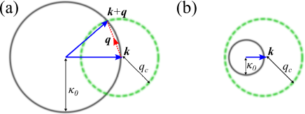
Figure 1: The black Ewald circle is the shell containing the loci of all possible $\bm{k}$ states such that $|\bm{k}|=\kappa_{0}$. The green circle of radius $q_{\text{c}}$ is centered at $\bm{k}$ and contains the loci of all the possible $\bm{q}$ disorder Fourier components in the Berry potential. (a) If $\kappa_{0}>q_{\text{c}}/2$, then the on-shell $\bm{k}\rightarrow\bm{k}+\bm{q}$ scattering process is allowed because the two circles intersect. (b) If $\kappa_{0}<q_{\text{c}}/2$, then the two circles do not intersect and there is no on-shell scattering.

II.4.2 Selective transparency

Beyond isotropic transparency, we can also fine-tune $\mathcal{V}(\bm{q})$ to generate wave transparency for a set of $\bm{k}$ plane-wave states that is more selective than the $0<\omega<\omega_{\text{c}}$ frequency band in isotropic transparency. Instead of setting $\mathcal{V}(\bm{q})=0$ in the entire $|\bm{q}|<q_{\text{c}}$ neighborhood, we limit the $\mathcal{V}(\bm{q})=0$ condition to a subset of the Fourier components in the $|\bm{q}|<q_{\text{c}}$ region to generate a smaller window of wave transparency containing the selected $\bm{k}$ plane-wave states. In other words, we permit some non-zero Fourier components in the ‘exclusion zone’ to interact (scatter) with the incoming plane-wave states that are outside of this window. To do this, we need to determine the condition for $\mathcal{P}_{n}(\bm{k},\bm{r})=0$ for the $\bm{k}$ states in this window. We first show how this is determined for $\mathcal{P}_{1}(\bm{k},\bm{r})$ in Eq. (11), which is associated with the $\bm{k}\stackrel{{\scriptstyle\mathcal{V}(\bm{q}_{1})}}{{\longrightarrow}}\bm{k}+\bm{q}_{1}$ scattering processes of an individual $\bm{k}$ state, as the procedure can be generalized to higher-order $\mathcal{P}_{n}(\bm{k},\bm{r})$ terms because the integrand for $\mathcal{P}_{n}(\bm{k},\bm{r})$ in Eq. (16) also contains the $\mathcal{V}(\bm{q})\mathcal{G}_{0}^{+}(\bm{k}+\bm{q})$ term which determines the loci of $\bm{q}$ for the $\mathcal{V}(\bm{q})$ contributing to the integral.

Given the presence of the $\mathcal{V}(\bm{q})\mathcal{G}_{0}^{+}(\bm{k}+\bm{q})$ term in the integrand, which we associate with the $\bm{k}\rightarrow\bm{k}+\bm{q}$ scattering process shown in Fig. 1(a), we minimize the integral in Eq. (11) and hence $\mathcal{P}_{1}(\bm{k},\bm{r})$ by setting $\mathcal{V}(\bm{q})=0$ for all possible values of $\bm{q}$ that satisfy $|\bm{k}+\bm{q}|=\kappa_{0}$. These loci of $\bm{q}$ values for $\mathcal{V}(\bm{q})=0$ comprise a circle of radius $\kappa_{0}$ centered at $\bm{q}=-\bm{k}$ in reciprocal space and contain all the Fourier components that can interact with that particular $\bm{k}$ state. For each $\bm{k}$ state, we have one circle. We note that this circle is contained within the $|\bm{q}|<2\kappa_{0}$ neighborhood. Hence, to generate transparency for a window of $\bm{k}$ states, we set the $\mathcal{V}(\bm{q})=0$ condition over the reciprocal-space region defined by the superposition of these circles. If this transparency window includes all the $\bm{k}$ states with $|\bm{k}|<q_{\text{c}}/2$ like in SH systems, then, as expected, we have to impose the $\mathcal{V}(\bm{q})=0$ condition over the entire $|\bm{q}|<q_{\text{c}}$ neighborhood. Otherwise, the $\mathcal{V}(\bm{q})=0$ condition has to be applied to only a subregion of the $|\bm{q}|<q_{\text{c}}$ neighborhood. This procedure also minimizes the higher-order $\mathcal{P}_{n}(\bm{k},\bm{r})$ terms, which are associated with the $\bm{k}\stackrel{{\scriptstyle\mathcal{V}(\bm{q}_{1})}}{{\longrightarrow}}\bm{k}+\bm{q}_{1}\stackrel{{\scriptstyle\mathcal{V}(\bm{q}_{2})}}{{\longrightarrow}}\ldots\stackrel{{\scriptstyle\mathcal{V}(\bm{q}_{n})}}{{\longrightarrow}}\bm{k}+\bm{q}_{1}+\ldots+\bm{q}_{n}$ process for multiple scattering, because it suppresses the $\bm{k}\stackrel{{\scriptstyle\mathcal{V}(\bm{q}_{1})}}{{\longrightarrow}}\bm{k}+\bm{q}_{1}$ part of the scattering process.

This result can be reached from another perspective by considering the self-energy, which describes the frequency shift and inverse lifetime caused by the disorder scattering, as defined by $\Sigma(\omega,\bm{k})=\mathcal{G}_{0}^{+}(\bm{k})^{-1}-\langle\mathcal{G}(\bm{k})\rangle^{-1}$ where $\langle\mathcal{G}(\bm{k})\rangle$ is the configuration-averaged disordered Green’s function in reciprocal space. To the lowest non-zero $O(\alpha^{2})$ approximation, we can write (Mahan, 2000)

$$\Sigma(\omega,\bm{k}) \approx\int\frac{d\bm{q}}{(2\pi)^{2}}\langle\mathcal{V}(\bm{q})\mathcal{V}(-\bm{q})\rangle\mathcal{G}_{0}^{+}(\bm{k}+\bm{q})$$

$$\approx\int\frac{d\bm{q}}{(2\pi)^{2}}|\mathcal{V}(\bm{q})|^{2}\mathcal{G}_{0}^{+}(\bm{k}+\bm{q})$$ (18)

since $\mathcal{V}(-\bm{q})=\mathcal{V}(\bm{q})^{\dagger}$. Given the singularity in $\mathcal{G}_{0}^{+}(\bm{k}+\bm{q})$ and the linear dispersion $\omega(\bm{k})=c|\bm{k}|$, the $\bm{q}$ integral for $\Sigma(\omega,\bm{k})$ is effectively taken over a circular shell of radius $\kappa_{0}$ centered at $\bm{q}=-\bm{k}$ in reciprocal space, like in the integral for $\mathcal{P}_{1}(\bm{k},\bm{r})$ in Eq. (11). Therefore, if we set $\mathcal{V}(\bm{q})=0$ on this shell and use the on-shell approximation $|\bm{k}|=\kappa_{0}$, then we have $\Sigma(\omega,\bm{k})\approx 0$ which we interpret as the absence of scattering for the $\bm{k}$ plane-wave state.

III Coherent transmission simulation and analysis

III.1 Simulation setup

To validate our analysis, we compute the coherent transmission coefficient $t(\bm{k})$, (Anderson, 1985) which determines the proportion of the wave flux passing through the disordered region without blurring, for a range of $\bm{k}$ states. If $|t(\bm{k})|^{2}=1$, the disordered medium is completely transparent. We approximate Eq. (2) using a 2D square lattice (Sheng, 2006), in which the second derivatives are replaced by finite differences, i.e., $\nabla^{2}\psi(\bm{r})\approx\frac{1}{a^{2}}[-4\psi(\bm{r})+\psi(\bm{r}+a\hat{\bm{x}})+\psi(\bm{r}-a\hat{\bm{x}})-\psi(\bm{r}+a\hat{\bm{y}})+\psi(\bm{r}-a\hat{\bm{y}})]$ where $a$ is the 2D lattice constant determined by the length scale of the scattering problem. The resulting eigenvalue equation $\frac{1}{a^{2}}[4\psi(\bm{r})-\psi(\bm{r}+a\hat{\bm{x}})-\psi(\bm{r}-a\hat{\bm{x}})-\psi(\bm{r}+a\hat{\bm{y}})-\psi(\bm{r}-a\hat{\bm{y}})]=\omega^{2}\frac{\epsilon(\bm{r})}{c^{2}}\psi(\bm{r})$ can be written in the matrix form $\bm{K}\Psi=\omega^{2}\bm{M}\Psi$, where $\bm{K}$ is the finite-difference matrix, $\Psi$ is a column vector with $\psi(\bm{r})$ as its vector elements, and $\bm{M}$ is a diagonal matrix with $\frac{\epsilon(\bm{r})}{c^{2}}$ as its diagonal elements. This formulation sets us up for the direct scattering amplitude calculations using the AGF method, (Ong, 2018a, b) a technique developed to study phonon scattering. (Ong et al., 2020; Ong, 2021) In the disorder-free lattice where $\epsilon(\bm{r})=\epsilon_{0}$, the dispersion relationship is given by (Sheng, 2006) $\omega(\bm{k})^{2}=\frac{4c^{2}}{a^{2}}[\sin^{2}(\frac{1}{2}k_{x}a)+\sin^{2}(\frac{1}{2}k_{y}a)]$. In the continuum ($a\rightarrow 0$) limit, we obtain $|\bm{k}|=\kappa_{0}$ and recover the linear $\omega(\bm{k})=c|\bm{k}|$ relationship. (Sheng, 2006)

Our AGF simulation setup is shown in Fig. 2. A disordered region of width $W$ and length $L$ is sandwiched between the semi-infinite and disorder-free left and right leads where $f(\bm{r})=0$. We fix $W=200a$ and let $L$ vary. We use the dimensionless variable $\kappa_{0}a$ to represent the frequency. For each $\bm{k}$ plane wave, we compute $|t(\bm{k})|^{2}=|S(\bm{k},\bm{k})|^{2}$, where $S(\bm{k}^{\prime},\bm{k})$ is the scattering amplitude between the incoming state $\Psi_{\text{in}}(\bm{k})$ and the outgoing state $\Psi_{\text{out}}(\bm{k}^{\prime})$ at frequency $\omega$. At each frequency step, we determine all the kinematically allowed $\bm{k}$ states and compute their $S(\bm{k}^{\prime},\bm{k})$ and $|t(\bm{k})|^{2}$ values. For consistency with our analysis based on the continuum limit, we restrict the range of $\bm{k}$ in our AGF calculations to $|\bm{k}|\apprle 1/a$ or $\kappa_{0}a\leq 1$.

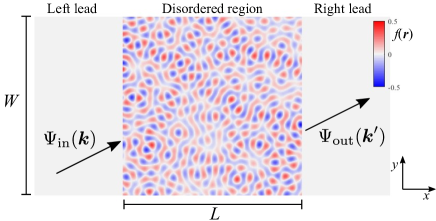
Figure 2: Schematic of the simulation setup for the AGF calculations. The disordered region ($0\leq x\leq L$) is confined between the two semi-infinite disorder-free leads on the left ($x<0$) and right ($x>L$) where $f(\bm{r})=0$. In the transverse $y$ direction, we impose periodic boundary conditions.

III.2 Simulation results

III.2.1 Isotropic wave transparency

Figure 3(a) shows an instance of $f(\bm{r})$ in which its Fourier components are distributed uniformly over a circular manifold (or ‘ring’) with a radius of $|\bm{q}|=q_{\text{c}}=0.5/a$, as shown in the inset of Fig. 3(a). The corresponding $|t(\bm{k})|^{2}$ spectrum for $L=5W$ is shown in Fig. 3(b) for the frequency range $0<\kappa_{0}a\leq 1$. We observe that for $\kappa_{0}>q_{\text{c}}/2$, $|t(\bm{k})|^{2}\approx 0$ for almost every state as a result of multiple scattering by the disorder. This reduction in $|t(\bm{k})|^{2}$ for $\kappa_{0}>q_{\text{c}}/2$ is a result of the disordered domain being much larger than the mean free paths of the plane-wave states with $\kappa_{0}>q_{\text{c}}/2$. At $\kappa_{0}=q_{\text{c}}/2$, there is a sharp transition or cutoff frequency, below which $|t(\bm{k})|^{2}\approx 1$ or near-perfect transparency for every state regardless of the angle of incidence. Nonetheless, we observe some speckling in the $|t(\bm{k})|^{2}$ spectrum above the cutoff frequency due to the random phase in the disorder modes. If we distribute the disorder components uniformly over a band of rings ($0.5/a\leq|\bm{q}|\leq 1/a$), as shown in the inset of Fig. 3(c), instead of a single ring, then the speckling is smoothed out, as shown in Fig. 3(d), because of the greater range of $\mathcal{V}(\bm{q})$ components available for on-shell scattering.

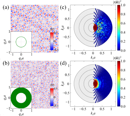
Figure 3: The disorder function $f(\bm{r})$ for disorder modes at (a) $|\bm{q}|=0.5/a$ and (b) $0.5/a\leq|\bm{q}|\leq 1/a$. The value of $f(\bm{r})$ is indicated by the color bar in the bottom right corner. The bottom left corner insets show the loci of the disorder modes in $\bm{q}$ space. The corresponding coherent transmission $|t(\bm{k})|^{2}$ spectra for $L=5W$ are shown in (c) and (d), respectively, with each $\bm{k}$ plane wave represented by a colored dot indicating its numerical value according to the color bar. To guide the eye, we draw the dimensionless frequency-dependent $\kappa_{0}a$ contour lines at intervals of $0.025$ (gray lines) and $0.25$ (black lines).

III.2.2 Orientation and frequency-dependent transparency window

The smoothing of the speckling in Fig. 3(d) implies that the the effects of the disorder Fourier components are additive, i.e., by selectively including more Fourier components in $f(\bm{r})$ we can introduce more scattering pathways to modify the $|t(\bm{k})|^{2}$ spectrum by filtering out unwanted $\bm{k}$ states. We go beyond the SH systems by introducing an anisotropic substructure in the distribution of the Fourier components. We elaborate on this idea with the example in Fig. .4. Figure 4(a) shows the anisotropic $f(\bm{r})$ distribution ($f=f_{\text{inner}}+f_{\text{outer}}$) obtained from combining two disorder distributions $f_{\text{inner}}(\bm{r})$ and $f_{\text{outer}}(\bm{r})$, shown in Figs. 4(b) and (c), respectively. Each of the disorder distributions corresponds to a set of distinctive scattering pathways. The highly anisotropic $f_{\text{inner}}$ comprises Fourier components distributed over two circular pockets with radius of $0.2/a$ and centered away from the origin at $q_{x}=\pm 0.3/a$ unlike the examples in Fig. 3. On the other hand, $f_{\text{outer}}$, which describes SH-like disorder, is isotropic and comprises Fourier components that are centered at the origin and distributed over a band of rings with radii varying between $1/a$ and $1.5/a$.

To understand how combining disorder distributions affects the scattering pathways, we plot in Figs. 4(d) to (f) the $\bm{k}$ plane-wave states that are unaffected by on-shell scattering for $f(\bm{r})$, $f_{\text{inner}}(\bm{r})$, and $f_{\text{outer}}(\bm{r})$, respectively. At each given $\kappa_{0}$, we compute all the possible $\bm{k}\rightarrow\bm{k}+\bm{q}$ on-shell scattering transitions for each $\bm{k}$ state. If none of the $\bm{q}$’s lie in the region occupied by the Fourier components, then that $\bm{k}$ state is considered unaffected by on-shell scattering. The distribution of unscattered $\bm{k}$ states for $f_{\text{inner}}$ in Fig. 4(e) shows a distinctive anisotropy. At more oblique angles of incidence, the $\bm{k}$ states are more likely to be scattered. The low-frequency plane waves with $\kappa_{0}a<0.05$ are however unaffected by on-shell scattering because the disorder component closest to the origin is at $\bm{q}=(\pm 0.1/a,0)$. In the $0.05\leq\kappa_{0}a\leq 0.25$ frequency range, there is a transmission gap because of the absence of unscattered plane waves. The upper bound of this gap is determined by the position of the disorder mode furthest from the origin at $\bm{q}=(\pm 0.5/a,0)$ and can be adjusted by changing the radius and position of the circular pockets in $f_{\text{inner}}$. At higher frequencies ($\kappa_{0}a>0.25$), a range of unscattered $\bm{k}$ states exists for more acute incident angles because there are no disorder modes available in $f_{\text{inner}}$ to scatter the plane wave at higher frequencies for small incident angles. For $f_{\text{outer}}$, the distribution of unscattered $\bm{k}$ states in Fig. 4(f) show a sharp cutoff at $\kappa_{0}a<0.5$ because the disorder Fourier components are located in the $1/a\leq|\bm{q}|\leq 1.5/a$ band.

Hence, for $f$, Fig. 4(d) shows the distribution of unscattered $\bm{k}$ states, which is equal to the intersection of the unscattered $\bm{k}$ states in Figs. 4(e) and (f). Figures 4(g) to (i) show the $|t(\bm{k})|^{2}$ spectra for $L=20W$ where a larger $L$ is chosen to magnify the effects of multiple scattering. We see a close correspondence between Figs. 4(d) and (g), with the $|t(\bm{k})|^{2}$ values highest for the unscattered $\bm{k}$ states, validating our theory of how disorder Fourier components affect wave scattering and transport. The $|t(\bm{k})|^{2}$ spectrum for $f$ can also be approximated by taking the product of the $|t(\bm{k})|^{2}$’s for $f_{\text{inner}}$ and $f_{\text{outer}}$ from Figs. 4(h) and (i). Figure 4(g) shows that by combining the Fourier components of $f_{\text{inner}}$ and $f_{\text{outer}}$ to filter out the unwanted $\bm{k}$ states, we are able to create transmission gaps and a window of high transparency [Fig. 4(g)] in the $|t(\bm{k})|^{2}$ spectrum, in which incoming plane waves can be robustly transmitted through the disordered medium without blurring. The correspondence between Figs. 4(d) and (g) is however not perfect because of wave reflection at the boundary between the leads and the disordered region. Nevertheless, the example from Fig. 4 shows that we can combine groups of disorder Fourier components to engineer specific wave transport properties such as the transparency window; we use $f_{\text{in}}$ to create anisotropy and a transmission gap and $f_{\text{out}}$to create a low-pass filter. Furthermore, the orientation, size and position of the transparency window can be modified by changing the loci of the circular pockets and ring in $f$. In Figs. 6 and 7, we also show how the $|t(\bm{k})|^{2}$ spectrum changes when we modify $f_{\text{inner}}$ by changing the orientation of the circular pockets.

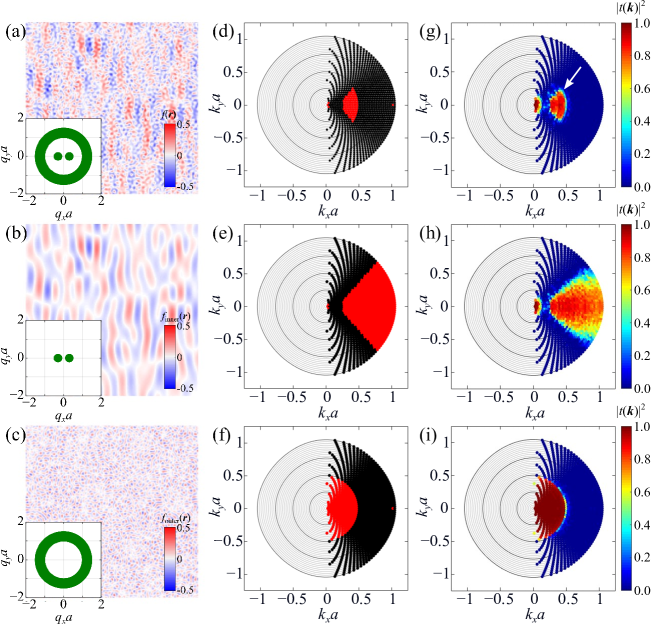
Figure 4: Plot of the disorder function for (a) $f(\bm{r})$, (b) $f_{\text{inner}}(\bm{r})$, and (c) $f_{\text{outer}}(\bm{r})$. The value of $f(\bm{r})$ is indicated by the color bar in the bottom right corner. The bottom left corner insets show the loci of the Fourier components in $\bm{q}$ space. The corresponding distributions of the scattered (black dots) and unscattered (red dots) $\bm{k}$ plane-wave states are shown in (d) to (f) while the $|t(\bm{k})|^{2}$ spectra for $L=20W$ are shown in (g) to (i) with the numerical values represented by the color bar. The white arrow in (g) points to the window of transparency for $f(\bm{r})$.

For greater clarity, we plot in Fig. 5 the coherent transmission $|t(\bm{k})|^{2}$ spectrum from Fig. 4(g) for incoming plane-wave states at normal incidence ($k_{y}=0$). We observe two transmission bands – one at low frequencies ($\kappa_{0}a<0.05$) and the other in the ‘window’ ($0.25<\kappa_{0}a<0.5$). The two transmission bands are separated by a ‘mid gap’ ($0.05\leq\kappa_{0}a\leq 0.25$) that originates from scattering by the Fourier components associated with $f_{\text{inner}}$ while the ‘window’ is bounded from above by a ‘top gap’ ($\kappa_{0}a\geq 0.5$) originating from scattering by the Fourier components associated with $f_{\text{outer}}$.

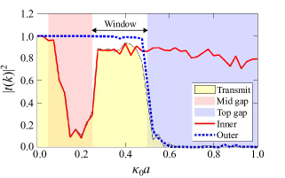
Figure 5: Coherent transmission $|t(\bm{k})|^{2}$ spectrum (yellow shaded area under the curve) for the disorder function $f(\bm{r})$ as a function of frequency $\kappa_{0}a$ at normal incidence ($k_{y}=0$) with the label ‘Transmit’. The spectrum is derived from Fig. 4(g). The $|t(\bm{k})|^{2}$ spectra for $f_{\text{inner}}$ and $f_{\text{outer}}$ are labeled ‘Inner’ (red solid line) and ‘Outer’ (dashed blue line), respectively, with the corresponding transmission gaps labeled ‘Mid gap’ (red shaded rectangle) and ‘Top gap’ (blue shaded rectangle). The transmission window in the $0.25<\kappa_{0}a<0.5$ range is indicated by the double-headed arrow (‘Window’).

III.3 Possible experimental realization

This phenomenon can be simulated for TM waves in a 2D photonic crystal (PC) with tunable site disorder. A prototype would be a 2D square lattice of cylindrical dielectric rods (Istrate and Sargent, 2006; Busch et al., 2007) with a radius of $R$ and nearest-neighbor distance of $h$. To realize the spatial structure of the disorder described by $f(\bm{r})$, we can let the cylinder radius be site dependent, i.e., $R(\bm{r})=R_{0}[1+f(\bm{r})]$, where $R_{0}$ is the average radius of the rods in the photonic crystal, so that the perturbation is proportional to $f(\bm{r})$. The coherent transmission spectrum through a disordered PC sandwiched between two disorder-free PC leads as in Fig. 2 should be similar to those in Fig. 3. Alternatively, the coherent transmission spectrum should be observed in a disordered PC with a position-dependent refractive index. (Schwartz et al., 2007)

Another possible approach for experimental realization would be to allow the amplitude of the nonzero Fourier components of $f(\bm{r})$ to vary while we fix the loci of the zero-amplitude Fourier components in $\bm{q}$ space. For instance, in the example in Section III.2.2, the zero-amplitude Fourier components would be confined to the region surrounding the two circular pockets and bounded by the ring as shown in the inset of Fig. 4(a). This provides us with more flexibility in the design of disordered media with selective transparency and such disorder configurations can be realized through collective-coordinate optimization. (Uche et al., 2004; Torquato, 2018)

IV Summary

We have elucidated the role of disorder, in terms of its Fourier components, in wave scattering in a 2D disordered medium. We show how the disorder configuration, as determined by $\mathcal{V}(\bm{q})$, can be engineered for isotropic and selective wave transparency. Using numerical simulations, we demonstrate an approach where, by choosing the appropriate combination of Fourier components, wave scattering can be selectively suppressed and the transport properties of the material can be engineered to create transmission gaps and allow specific incident waves to be robustly and coherently transmitted in orientation-dependent frequency windows. This Fourier components-based approach, which requires neither nontrivial topological wave properties nor a non-Hermitian medium, can be generalized to tailor the transport properties of disordered media for fundamental investigations of disordered systems and applications in acoustics, imaging, photonics, and structural health monitoring.

Appendix A Coherent transmission spectra for other combinations of $f_{\text{inner}}$ and $f_{\text{outer}}$

We plot in Figs. 6 and 7 the simulation data for different $f_{\text{inner}}$. The data in Fig. 6 are for an $f_{\text{inner}}$ that is like the one in Fig. 4 but rotated by 45 degrees with respect to the $x$ axis. The coherent transmission spectra for $f$ and $f_{\text{inner}}$ are also rotated by 45 degrees with respect to the $x$ axis. Hence, we do not observe the window of transparency unless the angle of incidence is close to 45 degrees. Similarly, the data in Fig. 7 are for an $f_{\text{inner}}$ that is rotated by 90 degrees. Hence, the window of transparency can only be observed at very oblique angles of incidence close to 0 degree.

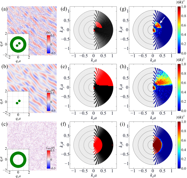
Figure 6: Plot of the disorder function for (a) $f(\bm{r})$, (b) $f_{\text{inner}}(\bm{r})$, and (c) $f_{\text{outer}}(\bm{r})$ with $f_{\text{inner}}$ rotated by 45 degrees. The value of $f(\bm{r})$ is indicated by the color bar in the bottom right corner. The bottom left corner insets show the loci of the disorder modes in $\bm{q}$ space. The corresponding distributions of the scattered (black dots) and unscattered (red dots) $\bm{k}$ plane-wave states are shown in (d) to (f) while the $|t(\bm{k})|^{2}$ spectra for $L=20W$ are shown in (g) to (i) with the numerical values represented by the color bar. The white arrow in (g) points to the window of transparency for $f(\bm{r})$.

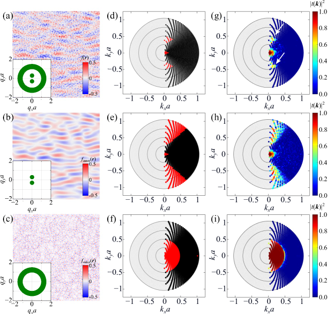
Figure 7: Plot of the disorder function for (a) $f(\bm{r})$, (b) $f_{\text{inner}}(\bm{r})$, and (c) $f_{\text{outer}}(\bm{r})$ with $f_{\text{inner}}$ rotated by 90 degrees. The value of $f(\bm{r})$ is indicated by the color bar in the bottom right corner. The bottom left corner insets show the loci of the disorder modes in $\bm{q}$ space. The corresponding distributions of the scattered (black dots) and unscattered (red dots) $\bm{k}$ plane-wave states are shown in (d) to (f) while the $|t(\bm{k})|^{2}$ spectra for $L=20W$ are shown in (g) to (i) with the numerical values represented by the color bar. The white arrows in (g) point to the window of transparency for $f(\bm{r})$.

References

- Lagendijk et al. (2009) Ad Lagendijk, Bart van Tiggelen, and Diederik S Wiersma, “Fifty years of Anderson localization,” Physics Today 62, 24–29 (2009).
- Modugno (2010) Giovanni Modugno, “Anderson localization in Bose–Einstein condensates,” Reports on Progress in Physics 73, 102401 (2010).
- Gredeskul et al. (2012) Sergey A Gredeskul, Yuri S Kivshar, Ara A Asatryan, Konstantin Y Bliokh, Yuri P Bliokh, Valentin D Freilikher, and Ilya V Shadrivov, “Anderson localization in metamaterials and other complex media (Review Article),” Low Temperature Physics 38, 570–602 (2012).
- Segev et al. (2013) Mordechai Segev, Yaron Silberberg, and Demetrios N Christodoulides, “Anderson localization of light,” Nature Photonics 7, 197–204 (2013).
- Mafi et al. (2019) Arash Mafi, John Ballato, Karl W Koch, and Axel Schülzgen, “Disordered Anderson Localization Optical Fibers for Image Transport—A Review,” Journal of Lightwave Technology 37, 5652–5659 (2019).
- Sheng (2006) Ping Sheng, Introduction to Wave Scattering, Localization and Mesoscopic Phenomena, 2nd ed. (Springer Berlin, Heidelberg, Heidelberg, Germany, 2006).
- Wiersma (2013) Diederik S Wiersma, “Disordered photonics,” Nature Photonics 7, 188–196 (2013).
- Yu et al. (2021) Sunkyu Yu, Cheng-Wei Qiu, Yidong Chong, Salvatore Torquato, and Namkyoo Park, “Engineered disorder in photonics,” Nature Reviews Materials 6, 226–243 (2021).
- Cao et al. (2022) Hui Cao, Allard Pieter Mosk, and Stefan Rotter, “Shaping the propagation of light in complex media,” Nature Physics 18, 994–1007 (2022).
- Bertolotti and Katz (2022) Jacopo Bertolotti and Ori Katz, “Imaging in complex media,” Nature Physics 18, 1008–1017 (2022).
- Gigan (2022) Sylvain Gigan, “Imaging and computing with disorder,” Nature Physics 18, 980–985 (2022).
- Maynard (2001) J D Maynard, “Acoustical analogs of condensed-matter problems,” Rev. Mod. Phys. 73, 401–417 (2001).
- Billy et al. (2008) Juliette Billy, Vincent Josse, Zhanchun Zuo, Alain Bernard, Ben Hambrecht, Pierre Lugan, David Clement, Laurent Sanchez-Palencia, Philippe Bouyer, and Alain Aspect, “Direct observation of Anderson localization of matter waves in a controlled disorder,” Nature 453, 891–894 (2008).
- Zangeneh-Nejad and Fleury (2020) Farzad Zangeneh-Nejad and Romain Fleury, “Disorder-Induced Signal Filtering with Topological Metamaterials,” Advanced Materials 32, 2001034 (2020).
- Kim and Heller (2022) Donghwan Kim and Eric J Heller, “Bragg Scattering from a Random Potential,” Phys. Rev. Lett. 128, 200402 (2022).
- Note (1) In our paper, we use the letters and to denote the wave vectors of the plane-wave states and disorder Fourier components, respectively.
- Note (2) For convenience, we use the term ‘components’ to label the plane-wave components of the disorder. We reserve the term ‘state’ for the plane-wave solutions to the Helmholtz wave equation.
- Note (3) Equation (1) also includes the contribution of the component at for .
- (19) Kevin Vynck, Romain Pierrat, Rémi Carminati, Luis S Froufe-Pérez, Frank Scheffold, Riccardo Sapienza, Silvia Vignolini, and Juan José Sáenz, “Light in correlated disordered media,” Rev. Mod. Phys. (in press) arXiv:2106.13892 .
- Leseur et al. (2016) O Leseur, R Pierrat, and R Carminati, “High-density hyperuniform materials can be transparent,” Optica 3, 763–767 (2016).
- Torquato (2018) Salvatore Torquato, “Hyperuniform states of matter,” Physics Reports 745, 1–95 (2018).
- Torquato (2016) Salvatore Torquato, “Hyperuniformity and its generalizations,” Phys. Rev. E 94, 22122 (2016).
- Kim and Torquato (2020) J Kim and S Torquato, “Effective elastic wave characteristics of composite media,” New J. Phys. 22, 123050 (2020).
- Torquato and Kim (2021) Salvatore Torquato and Jaeuk Kim, “Nonlocal Effective Electromagnetic Wave Characteristics of Composite Media: Beyond the Quasistatic Regime,” Phys. Rev. X 11, 21002 (2021).
- Frank and Lubatsch (2011) Regine Frank and Andreas Lubatsch, “Scalar wave propagation in random amplifying media: Influence of localization effects on length and time scales and threshold behavior,” Phys. Rev. A 84, 13814 (2011).
- Sheremet et al. (2020) A Sheremet, R Pierrat, and R Carminati, “Absorption of scalar waves in correlated disordered media and its maximization using stealth hyperuniformity,” Phys. Rev. A 101, 53829 (2020).
- Anderson (1985) Philip W Anderson, “The question of classical localization A theory of white paint?” Philosophical Magazine B 52, 505–509 (1985).
- Ong (2018a) Zhun-Yong Ong, “Tutorial: Concepts and numerical techniques for modeling individual phonon transmission at interfaces,” J. Appl. Phys 124, 151101 (2018a).
- Ong (2018b) Zhun-Yong Ong, “Atomistic -matrix method for numerical simulation of phonon reflection, transmission, and boundary scattering,” Phys. Rev. B 98, 195301 (2018b).
- Davy et al. (2015) Matthieu Davy, Zhou Shi, Jongchul Park, Chushun Tian, and Azriel Z Genack, “Universal structure of transmission eigenchannels inside opaque media,” Nature Communications 6, 6893 (2015).
- Froufe-Pérez et al. (2017) Luis S Froufe-Pérez, Michael Engel, Juan José Sáenz, and Frank Scheffold, “Band gap formation and Anderson localization in disordered photonic materials with structural correlations,” Proc. Natl. Acad. Sci. U.S.A. 114, 9570–9574 (2017).
- Brandstötter et al. (2019) Andre Brandstötter, Adrian Girschik, Philipp Ambichl, and Stefan Rotter, “Shaping the branched flow of light through disordered media,” Proc. Natl. Acad. Sci. U.S.A. 116, 13260–13265 (2019).
- Economou (1983) Eleftherios N Economou, Green’s functions in quantum physics, 3rd ed. (Springer, Berlin, 1983).
- Note (4) In two dimensions, where denotes the zeroth-order Hankel function of the first kind. (Economou, 1983; Sheng, 2006).
- Mahan (2000) Gerald D Mahan, Many-Particle Physics (Springer-Verlag, Boston, MA, 2000).
- Ong et al. (2020) Zhun Yong Ong, Georg Schusteritsch, and Chris J. Pickard, “Structure-specific mode-resolved phonon coherence and specularity at graphene grain boundaries,” Phys. Rev. B 101, 195410 (2020), arXiv:2004.07424 .
- Ong (2021) Zhun Yong Ong, “Specular transmission and diffuse reflection in phonon scattering at grain boundary,” EPL 133, 66002 (2021), arXiv:2103.06444 .
- Note (5) We define the transmission gap as the frequency range in which plane waves cannot propagate through the disordered medium.
- Istrate and Sargent (2006) Emanuel Istrate and Edward H Sargent, “Photonic crystal heterostructures and interfaces,” Rev. Mod. Phys. 78, 455–481 (2006).
- Busch et al. (2007) K Busch, G von Freymann, S Linden, S F Mingaleev, L Tkeshelashvili, and M Wegener, “Periodic nanostructures for photonics,” Physics Reports 444, 101–202 (2007).
- Schwartz et al. (2007) Tal Schwartz, Guy Bartal, Shmuel Fishman, and Mordechai Segev, “Transport and Anderson localization in disordered two-dimensional photonic lattices,” Nature 446, 52–55 (2007).
- Uche et al. (2004) Obioma U Uche, Frank H Stillinger, and Salvatore Torquato, “Constraints on collective density variables: Two dimensions,” Phys. Rev. E 70, 46122 (2004).