Bistable wavefronts in the delayed Belousov-Zhabotinsky reaction

Abstract

We study the Murray adaptation of the Noyes-Field five-step model of the Belousov-Zhabotinsky (BZ) reaction in the case when a tuning parameter $r$, which determines the level of the bromide ion far ahead of the propagating wave, is bigger than 1 and when the delay in generation of the bromous acid is taken into account. The existence of wavefronts in the delayed BZ system was previously established only in the monostable situation with $r\in(0,1]$, the physically relevant bistable situation where $r>1$ (in real experiments $r$ varies between 5 and 50) was left open. We complete the study by showing that the BZ system with $r>1$ admits monotone traveling fronts. Note that one of the stable equilibria of the BZ model is not isolated. This circumstance does not allow the direct application of the topological or analytical methods previously elaborated for the analysis of the existence of bistable waves.

35C07, 35R10, 35K57

1 Introduction

Adapting the Noyes-Field five-step model [17] to describe the propagation of wave bands in the Belousov-Zhabotinsky (BZ for short) reaction, J.D. Murray in [15, 16] proposed the reaction-diffusion system

(1) $$\begin{array}[]{ll}u_{t}(t,x)=D_{u}\Delta u(t,x)+u(t,x)(1-u(t,x)-w(t-h,x)),&\\ w_{t}(t,x)=D_{w}\Delta w(t,x)-bu(t,x)w(t,x),\ u,w\geq 0,\ x\in{\mathbb{R}}^{2},&\end{array}$$

(with $h=0$) to describe planar waves $(u,w)=(\phi,\theta)(\nu\cdot x+ct)$, $(\phi,\theta)(-\infty)=(0,r),$ $(\phi,\theta)(+\infty)=(1,0),$ $r,b,D_{u},D_{w}\geq 0,\|\nu\|=1$, $0\leq u\leq 1,\ 0\leq w\leq r,$ propagating in a thin layer of reactant solution filled in a Petri plate. The variables $u,w$ are dimensionless and proportional to the bromous acid and bromide ion concentrations, respectively. See [6, 15, 16, 18] for the derivation of the model (1) (without delay) and the chemistry around it. A positive delay $h$ was later incorporated in (1) by J. Wu and X. Zou [28], paper [23] provides additional motives for this inclusion.

In order to visualise the quasi-monotonicity properties of (1), it is convenient to introduce a new variable $v=1-w$. Then, assuming that $D_{u}=D_{w}=1$ and that the level $r$ of concentration $w$ of the bromide ion far ahead of the propagating wave is known and fixed (in the real experiments $r$ can vary from 5 to 50, $b$ can take values from 2.5 to 12.5 [15]), we transform (1) into the system

(2) $$\begin{array}[]{ll}u_{t}(t,x)=\Delta u(t,x)+u(t,x)(1-r-u(t,x)+rv(t-h,x)),&\\ v_{t}(t,x)=\Delta v(t,x)+bu(t,x)(1-v(t,x)),\ u,v\in[0,1],\ \ x\in{\mathbb{R}}^{2},&\end{array}$$

and look for the non-negative wave solutions $(u,v)(t,x)=(\phi,\psi)(\nu\cdot x+ct)$ satisfying the normalised boundary conditions $(\phi,\psi)(-\infty)=(0,0),(\phi,\psi)(+\infty)=(1,1)$ and $0\leq\phi\leq 1,\ 0\leq\psi\leq 1$. It is known [9, 22] that the profiles $\phi(s),\psi(s)$ of such wavefronts (if they exist) are strictly monotone functions: in fact, $\phi^{\prime}(s),\psi^{\prime}(s)>0$ for all $s\in{\mathbb{R}}$. Importantly, the value of $r$ determines the mathematical nature of the BZ system. Namely, if $r\in(0,1)$, the system (1) is monostable non-degenerate and is monostable degenerate when $r=1$; on the other hand, with $r>1$ the BZ system is bistable [22]. Note that the standard mono- and bi-stability definitions [25, p. 158] require the stability analysis of steady states of the following system

(3) $$\begin{array}[]{ll}\phi^{\prime}(t)=\phi(t)(1-r-\phi(t)+r\psi(t-h)),&\\ \psi^{\prime}(t)=b\phi(t)(1-\psi(t)),\ (\psi,\phi)\in[0,1]\times[0,1].&\end{array}$$

describing spatially homogeneous solutions for (2). It is easy to see that the spectra of linearizations of (3) at $(0,0)$ and $(1,1)$ are $\{0,1-r\}$ and $\{-1,-b\}$, respectively. Thus the equilibrium $(1,1)$ is exponentially stable independently on the size of the positive parameters $h,b,r$. Since the equilibrium $(0,0)$ is not isolated, its analysis is more delicate: see Appendix A where the (non-asymptotical) stability of solution $(0,0)$ for (3) with $r>1$ is proven.

The local and non-delayed case ($h=0$) is simpler to study since it allows the plane phase analysis to find the bistable waves. This technically substantial work was realised by Y. Kanel in [11]. It was preceded by the abundant numerical evidences for the presence of bistable fronts in the non-delayed BZ system [13, 15, 16, 19] and by the theoretical work of R.G. Gibbs [6]. In the latter paper, on the base of geometrical-analytical arguments, the existence [respectively, non-existence] of bistable waves for (1) admitting only diffusion in bromous acid, $D_{u}=1,D_{w}=0$ [respectively, admitting only diffusion in bromide ion, $D_{u}=0,D_{w}=1$] was established. It is also worth to mention here the recent study by H.-T. Niu et al [18] where the existence of V-shaped traveling fronts in (1) with $r>1,h=0$ was proved by constructing suitable super- and sub-solutions.

Now, the existence, stability and uniqueness of wavefronts in the BZ system with spatiotemporal interactions (which includes (1) as a particular case) was previously analysed only in the monostable situation $r\in(0,1]$ under different conditions imposed on the parameters $c,h,r,b$ or interaction kernels, see [1, 3, 8, 9, 12, 22, 23, 24, 25, 27, 28, 29] and the references therein. The chemically relevant bistable case $r>1$ (recall that in real experiments $r$ varies between 5 and 50) was left open. We believe that one of the main reasons of such a circumstance is that the stable equilibrium $(0,0)$ of the quasi-monotone BZ model (2) is not isolated. This does not allow the direct application of topological or analytical methods previously elaborated for the analysis of the existence of bistable waves in the monotone non-local or delayed systems (see [4, 26] for more references). In this paper, we propose a different approach to complete the study by showing that the delayed BZ system with $r>1$ admits monotone traveling fronts. As a by-product, we obtain an alternative proof for the above mentioned Kanel result [11, Theorem 4] concerning the existence of bistable fronts in the non-delayed BZ model. Our main conclusion is the following:

Theorem 1.1.

For every $r>1,b>0,h\geq 0,$ there exists a unique $c_{\star}=c_{\star}(b,r,h)$ for which system (2) admits a wavefront $(u,v)(t,x)=(\phi,\psi)(\nu\cdot x+c_{\star}t)$. Furthermore, $\phi^{\prime}(t)>0,$ $\psi^{\prime}(t)>0$, $\phi(t)<\psi(t)$ for all $t\in{\mathbb{R}}$ and $c_{\star}\in(0,2)$.

It should be noted that the last three inequalities in the above statement and the properties of the uniqueness and positivity of $c_{\star}$ were already proven in [22]. Nevertheless, we include this information in the theorem to draw more complete picture of bistable wavefronts in the BZ system.

Consequently, Theorem 1.1 will be proved if we establish the existence of positive wavefronts. We will reach this goal by approximating (2) with the perturbed system (6), see Section 2, parametrised by a small positive parameter $\epsilon$. We show that for each small $\epsilon>0$ perturbed equations have a monotone bistable wavefront $(u,v)=(\phi_{\epsilon},\psi_{\epsilon})$ traveling with a positive speed $c_{*}(\epsilon)$. The existence of such a wave is obtained by applying Fang and Zhao general theory of bistable waves for monotone evolution systems [4] to our particular situation. By itself, this application is not trivial and needs verifications of several fundamental hypotheses. The most complicated of them, in view of the bidimensional character of the system, is the counter-propagation property [4]. It can not be obtained as in the one-dimensional case, [4] and requires some additional ideas. We prove the counter-propagation by constructing appropriate sub-solutions and super-solutions in Appendices C and D. We hope that our approach can be useful in other similar situations. Next, in Section 3, we prove the existence of traveling waves by obtaining uniform a priori estimates for $c_{\star}$ and taking the limit of $(\phi_{\epsilon},\psi_{\epsilon})$ when $\epsilon\to 0^{+}$. Due to the degeneration of the equilibrium $(0,0)$, the latter task can be considered as the most difficult in the whole proof. We overcome this obstacle by tracking the evolution of $(\phi_{\epsilon},\psi_{\epsilon})$ as $\epsilon\to 0^{+}$ on the two-dimensional unstable manifold $\Gamma(\epsilon,c_{\epsilon}),\ \epsilon>0,$ of the equilibrium $(0,0)$. The existence and properties of $\Gamma(\epsilon,c_{\epsilon})$ are given in Theorem 3.1. The paper is concluded with 4 Appendices. We have already mentioned two of them, C and D. In addition, in Appendix A the bistable character of equation (3) is shown followed by the detailed analysis of the perturbed system and accompanied with phase space analysis numerical pictures. In Appendix B we are checking another fundamental hypothesis (the unordering property) for the theory in [4]. Again, the verification of this hypothesis is more difficult than in one-dimensional case due to the reducibility of matrices obtained from the linearisation of the perturbed system at its stable equilibria. See Subsection 2.1 for more details.

2 Monotone wavefronts for a perturbed BZ system

2.1 Perturbed BZ system: existence of monotone wavefronts

In order to prove Theorem 1.1, we have to solve the boundary value problem which consists from the differential equations for the wave profiles $\phi,\psi$:

(4) $$\begin{array}[]{ll}\phi^{\prime\prime}(t)-c\phi^{\prime}(t)+\phi(t)(1-r-\phi(t)+r\psi(t-ch))=0,&\\ \psi^{\prime\prime}(t)-c\psi^{\prime}(t)+b\phi(t)(1-\psi(t))=0,&\end{array}$$

and the boundary conditions $(\phi,\psi)(-\infty)=(0,0)$, $(\phi,\psi)(+\infty)=(1,1)$.

Solutions of the above problem will be obtained as limits (when $\epsilon\to+0$) of the positive wavefronts to the perturbed non-degenerate system

(5) $$\begin{array}[]{ll}\phi^{\prime\prime}(t)-c\phi^{\prime}(t)+\phi(t)(1-r-\phi(t)+r\psi(t-ch))=0,&\\ \psi^{\prime\prime}(t)-c\psi^{\prime}(t)+(b\phi(t)-\epsilon\psi(t))(1-\psi(t))=0.&\end{array}$$

Note that the whole evolution system is given by the system of two reaction-diffusion equations (with $\epsilon>0$)

(6) $$\begin{array}[]{ll}u_{t}(t,x)=u_{xx}(t,x)+u(t,x)(1-r-u(t,x)+rv(t-h,x)),&\\ v_{t}(t,x)=v_{xx}(t,x)+(bu(t,x)-\epsilon v(t,x))(1-v(t,x)),\ u,v\geq 0,\ x\in{\mathbb{R}}.&\end{array}$$

The proof of existence of wavefronts for (6) is our main goal in this subsection:

Theorem 2.1.

For every $b,h>0,r>1$ and sufficiently small positive $\epsilon$, the system (6) has a monotone bistable wavefront $u=\phi_{\epsilon}(x+c_{*}(\epsilon)t),\ v=\psi_{\epsilon}(x+c_{*}(\epsilon)t)$.

Proof 2.2.

We use the theory of abstract monotone bistable evolution systems developed in [4]. Thus we need to recall some definitions, notations and results from [4]. In particular, $\mathcal{X}^{+}$ stands for the subset $C([-h,0],[0,1]^{2})$ of the Banach lattice $C([-h,0],{\mathbb{R}}^{2})$ of continuous functions with the uniform norm and standard ordering of the elements. The standard order notation here is

$$(\phi_{2},\psi_{2})\geq(\phi_{1},\psi_{1})\quad\mbox{if}\quad\phi_{2}(s)\geq\phi_{1}(s),\ \psi_{2}(s)\geq\psi_{1}(s),\ s\in[-h,0],$$

$$(\phi_{2},\psi_{2})\gg(\phi_{1},\psi_{1})\quad\mbox{if}\quad\phi_{2}(s)>\phi_{1}(s),\ \psi_{2}(s)>\psi_{1}(s),\ s\in[-h,0].$$

Hence, if we set $\mathcal{C}:=C([-h,0]\times{\mathbb{R}},[0,1]^{2})$, then $\mathcal{C}$ can be regarded as the space of all continuous functions $\gamma:{\mathbb{R}}\to\mathcal{X}^{+}$. Using the latter interpretation of $\mathcal{C}$, we can equip this space with the metrizable topology of uniform convergence on compact subsets of ${\mathbb{R}}$. If $\gamma\in\mathcal{C}$ is a constant function we can identify it with an element $\gamma\in\mathcal{X}^{+}$. Let $\mathcal{C}_{\gamma}$ and $[O,\gamma]_{\mathcal{C}}$ [respectively, $\mathcal{X}_{\gamma}$] denote the set of all elements $\zeta\in\mathcal{C}$ [respectively, $\xi\in\mathcal{X}^{+}$] such that $0\leq\zeta(t)\leq\gamma(t)$ for all $t\in{\mathbb{R}}$ [respectively, $0\leq\xi\leq\gamma$].

Note that for each pair of non-negative continuous and bounded initial data $u(s,x)=u_{0}(s,x)\in[0,1],$ $v(s,x)=v_{0}(s,x)\in[0,1],$ $(s,x)\in[-h,0]\times{\mathbb{R}}$, system (6) has a unique continuous non-negative mild solution $(u,v)=(u(t,x),v(t,x))\in[0,1]^{2},x\in{\mathbb{R}},$ defined for all $t\geq 0$. Here the mild solutions are defined by means of the integral equations

$$u(t,x)=(S(t)u_{0})(x)+\int_{0}^{t}S(t-s)(u(s,\cdot)(M+1-r-u(s,\cdot)+rv(s-h,\cdot)))(x)ds,$$

$$v(t,x)=(S(t)v_{0})(x)+\int_{0}^{t}S(t-s)(Mv(s,\cdot)+(bu(s,\cdot)-\epsilon v(s,\cdot))(1-v(s,\cdot)))(x)ds,$$

with $M=2+r+br$ and the Gaussian-type action

$$(S(t)g)(x):=\frac{e^{-Mt}}{\sqrt{4\pi t}}\int_{-\infty}^{+\infty}e^{-(x-y)^{2}/(4t)}g(y)dy.$$

We observe that $(0,0)$ and $(1,1)$ are solutions of (6) and the integral operators are monotone with respect to the functions with values in the interval $[0,1]$. Therefore the comparison principle can be applied to the mild solutions of (6) (actually, in the sense of definitions in [4, 14, 20], the reaction term in (6) defines a quasi-monotone functional with values in $[0,1]^{2}$). Furthermore, partial derivatives $u_{x}(t,x),v_{x}(t,x)$ are continuous and bounded in the variable $x\in{\mathbb{R}}$ for each $t>0$; for instance,

$$|u_{x}(t,x)|\leq\frac{e^{-Mt}}{\sqrt{\pi t}}|u_{0}|_{\infty}+\int_{0}^{t}\frac{e^{-Ms}}{\sqrt{\pi s}}ds\sup_{x\in{\mathbb{R}},s\in[0,t]}|u(s,x)(3+br-u(s,x)+rv(s-h,x))|.$$

Thus (6) generates a continuous monotone semi-flow $\mathcal{Q}^{t}$ defined on the phase space $\mathcal{C}=C([-h,0]\times{\mathbb{R}},[0,1]^{2})$ by

$$\mathcal{Q}^{t}(u_{0},v_{0})(s,x)=(u(t+s,x),v(t+s,x)),\quad s\in[-h,0],\ x\in{\mathbb{R}}.$$

Actually, arguing as in the proof of Theorem 1 in [14] (see also [20, p. 517]), we see that $(u(t,x),v(t,x))$ is a classical solution of (3) for $t>h$. Therefore a mild monotone traveling wave $(u,v)(t,x)=(\phi,\psi)(x+ct)$ propagating with the speed $c$, i.e.

$$\mathcal{Q}^{t}(\phi,\psi)(s,x+cs)=(\phi,\psi)(x+c(t+s)),\quad s\in[-h,0],\ x\in{\mathbb{R}},$$

is a classical traveling wave.

The system (6) has 4 equilibria:

$$O:=(0,0),\quad\beta:=(1,1);\quad\alpha_{1}:=(0,1);\quad\alpha_{2}:=\left(\frac{\epsilon(r-1)}{br-\epsilon},\frac{b(r-1)}{br-\epsilon}\right).$$

We also consider the restriction of the evolution system $\mathcal{Q}^{t}$ on the subset of homogeneous initial data $\mathcal{X}_{\beta}$: if $(\phi_{0},\psi_{0})\in\mathcal{X}_{\beta}$ and $(\phi(t),\psi(t))=\mathcal{Q}^{t}(\phi_{0},\psi_{0})(0,0)$, then

(7) $$\begin{array}[]{ll}\phi^{\prime}(t)=\phi(t)(1-r-\phi(t)+r\psi(t-h)),&\\ \psi^{\prime}(t)=(b\phi(t)-\epsilon\psi(t))(1-\psi(t)).&\end{array}$$

The existence of the bistable wave will be obtained from the next proposition which essentially coincides with Theorems 3.4 and 5.1 in [4] adapted to our particular situation:

Proposition 2.3.

[4] Assume that for each $t>0$, the maps $\mathcal{Q}^{t}$ and $\mathcal{Q}=\mathcal{Q}^{1}$ satisfy the assumptions

• (A1) (Translation invariance) $T_{a}\mathcal{Q}^{t}=\mathcal{Q}^{t}T_{a},\ a\in{\mathbb{R}}$, where $T_{a}:\mathcal{C}\to\mathcal{C}$ is a spatial shift operator: $T_{a}(u_{0}(\cdot,\cdot),v_{0}(\cdot,\cdot))=(u_{0}(\cdot,\cdot+a),v_{0}(\cdot,\cdot+a))$.

• (A3) (Monotonicity) The semi-flow $\mathcal{Q}^{t}$ is order preserving.

• (A4’) (Weak compactness) There exists $s\in(0,h]$ such that:

  (i) $\mathcal{Q}[(u_{0},v_{0})](\theta,x)=(u_{0},v_{0})(\theta+s,x)$ whenever $\theta+s\leq 0$;

  (ii) For any $\epsilon\in(0,s)$, the set $\mathcal{Q}[C_{\beta}]|_{[-s+\epsilon,0]\times{\mathbb{R}}}$ is precompact;

  (iii) For any subset $J\subset C_{\beta}$ with $J(0,\cdot)\subset C({\mathbb{R}},[0,1])$ being precompact, the set $\mathcal{Q}[J]|_{[-s,0]\times{\mathbb{R}}}$ is precompact.

• (A5) (Bistability) For each fixed $t>0$, the fixed points $O$ and $\beta$ are strongly stable from above and below, respectively, for the map $\mathcal{Q}^{t}:{\mathcal{X}}_{\beta}\to{\mathcal{X}}_{\beta}$ and any two intermediate equilibria of $\mathcal{Q}^{t}:{\mathcal{X}}_{\beta}\to{\mathcal{X}}_{\beta}$ are unordered.

• (A6) (Counter-propagation) For each $j=1,2$, the time-one map $\mathcal{Q}$ is such that

  $$c_{-}^{*}(\alpha_{j},\beta)+c_{+}^{*}(O,\alpha_{j})>0,$$

  where $c_{+}^{*}(O,\alpha_{j})$ [$c_{-}^{*}(\alpha_{j},\beta)$] is the rightward [leftward, respectively] asymptotic speed of propagation in the monostable subsystem $\mathcal{Q}:[O,\alpha_{j}]_{\mathcal{C}}\to[O,\alpha_{j}]_{\mathcal{C}}$ [$\mathcal{Q}:[\alpha_{j},\beta]_{\mathcal{C}}\to[\alpha_{j},\beta]_{\mathcal{C}}$, respectively].

Then there exists $c\in{\mathbb{R}}$ such that $\{\mathcal{Q}^{t}\}_{t\geq 0}$ admits a nondecreasing traveling wave with speed $c$ connecting $O$ to $\beta$.

The translation invariance and monotonicity property follow easily from the integral equations, we note here that the coefficients of the system do not depend on $t$ and $x$. The proof of the weak compactness property is given in [4] (pages 2269-2270).

In the Appendix B, we analyse the dynamics of $\mathcal{Q}^{t}$ on $\mathcal{X}_{\beta}$. In particular, for each $t>0$, we show that any two intermediate equilibria $\gamma_{j}\not\in\{O,\beta\}$, $j=1,2$, of $\mathcal{Q}^{t}$ are unordered. Thus the last part of Assumption (A5) is satisfied and we only need to show that the equilibria $O$ and $\beta$ meet the stability part of Assumption (A5). Since the linear parts of (7) at $O$ and $\beta$ lead to the reducible matrices (cf. [21]), we cannot argue as in the proof of [4, Theorem 6.4]. In Claims 1 and 2 below we present our detailed proof of the required unilateral stabilities for $O$ and $\beta$.

Finally, in view of the bidimensional character of system (6), Assumption (A6) is the most complicated one. Note that the set of fixed points for all maps $\mathcal{Q}^{t}:\mathcal{X}_{\beta}\to\mathcal{X}_{\beta}$, $t>0$ is precisely $\mathcal{E}:=\{O,\alpha_{1},\alpha_{2},\beta\}$. This explains the number of inequalities in (A6) according to [4]. The first inequality ($j=1$) is easy to check since both speeds $c_{-}^{*}(\alpha_{1},\beta)$ and $c_{+}^{*}(O,\alpha_{1})$ can be easily calculated, see Claim 3. The second inequality ($j=2$), however, can not be verified following the techniques used in [4] for the one-dimensional case. Thus this case requires some additional ideas. In our paper, we prove the counter-propagation inequality for the interior fixed point $\alpha_{2}$ by constructing in Appendices C and D appropriate sub-solutions and super-solutions. This construction is used in Claim 4 below to establish the fulfilment of the Assumption (A6).

Claim 1: The steady state $O$ is strongly stable from above.

For $0<\epsilon<r-1$ and small positive $m$,

$$0<m\leq m_{0}:=e^{-0.5\epsilon h}\min\left\{0.25,\left(1-\frac{1}{r}-\frac{\epsilon}{2r}\right)\right\},$$

and $\eta\in(0,1]$, we set

$$\phi^{*}(t,\eta):=\eta\phi^{*}(t):=\frac{\eta\epsilon m}{3b}e^{-0.5\epsilon t},\ \psi^{*}(t,\eta):=\eta\psi^{*}(t):=\eta me^{-0.5\epsilon t}.$$

Then, for all $t\geq 0$, $(\phi^{*}(t,\eta),\psi^{*}(t,\eta))$ is a strict super-solution in the sense that

(8) $$\begin{array}[]{ll}(\phi^{*}(t,\eta))^{\prime}>\phi^{*}(t,\eta)(1-r-\phi^{*}(t,\eta)+r\psi^{*}(t-h,\eta)),&\\ (\psi^{*}(t,\eta))^{\prime}>(b\phi^{*}(t,\eta)-\epsilon\psi^{*}(t,\eta))(1-\psi^{*}(t,\eta)).&\end{array}$$

Consequently, the solution $(\phi(t,\eta),\psi(t,\eta))$ of the initial value problem

$$(\phi(s,\eta),\psi(s,\eta))=(\phi^{*}(s,\eta),\psi^{*}(s,\eta)),\ s\in[-h,0],$$

for (7) satisfies

$$(\phi(t,\eta),\psi(t,\eta))<(\phi^{*}(t,\eta),\psi^{*}(t,\eta)),\quad t>0.$$

Indeed, this inequality obviously holds for all small $t>0$, and if $d>0$ is the leftmost point where the inequality fails (for example, suppose that $\phi(d,\eta)=\phi^{*}(d,\eta)$, $\psi(s,\eta)\leq\psi^{*}(s,\eta),\ s\leq d$, then

$$\phi(d,\eta)(1-r-\phi(d,\eta)+r\psi(d-h,\eta))=\phi^{\prime}(d,\eta)\geq$$

$$(\phi^{*})^{\prime}(d,\eta)>\phi(d,\eta)(1-r-\phi(d,\eta)+r\psi^{*}(d-h,\eta)),$$

a contradiction).

Hence, for all $\sigma>0$, $s\in[-h,0]$, $\eta\in(0,1]$, it holds that

$$\mathcal{Q}^{\sigma}(\eta\phi^{*},\eta\psi^{*})(s,0)\leq(\eta\phi^{*},\eta\psi^{*})(\sigma+s,0)\ll\eta(\phi^{*},\psi^{*})(s).$$

Therefore, using terminology in [4, p. 2247], we can say that the steady state $O$ is strongly stable from above. $\square$

Claim 2: The steady state $\beta$ is strongly stable from below.

Introducing the change of variables $\tilde{\phi}(t)=1-\phi(t)$, $\tilde{\psi}(t)=1-\psi(t)$, we transform (7) (after suppressing the symbol ”tilde” over variables) into the system

(9) $$\begin{array}[]{ll}\psi^{\prime}(t)=\psi(t)(-b+\epsilon-\epsilon\psi(t)+b\phi(t)),&\\ \phi^{\prime}(t)=(r\psi(t-h)-\phi(t))(1-\phi(t)),&\end{array}$$

which essentially coincides with (7). Thus, arguing as above, we find that the exponential functions

$$\phi^{*}(t,\eta):=\eta\phi^{*}(t):=\eta mr^{2}e^{-\delta t},\ \psi^{*}(t,\eta):=\eta\psi^{*}(t):=\eta me^{-\delta t}$$

with

$$\eta\in(0,1],\quad 0<\delta<\min\left\{b-\epsilon,{{\frac{(r-1)\ln r}{r\ln r+(r-1)h}}}\right\},$$

$$0<m\leq m_{1}:=\frac{1}{r^{2}}\min\left(1-\frac{\delta+\epsilon}{b},1-\frac{r\delta}{r-e^{\delta h}}\right),$$

are strict super-solutions for (9). Consequently, the solution $(\phi(t,\eta),\psi(t,\eta))$ of the initial value problem $(\phi(s,\eta),\psi(s,\eta))=(\phi^{*}(s,\eta),\psi^{*}(s,\eta)),\ s\in[-h,0],$ for (9) satisfies

$$(\phi(t,\eta),\psi(t,\eta))<(\phi^{*}(t,\eta),\psi^{*}(t,\eta)),\quad t>0.$$

Therefore

$$(1-\phi(t,\eta),1-\psi(t,\eta))>(1-\phi^{*}(t,\eta),1-\psi^{*}(t,\eta)),\quad t>0,$$

so that for each $\sigma>0$, $s\in[-h,0]$, $\eta\in(0,1]$, it holds

$$\mathcal{Q}^{\sigma}(1-\eta\phi^{*},1-\eta\psi^{*})(s,0)=(1-\phi(\sigma+s,\eta),1-\psi(\sigma+s,\eta))\geq$$

$$(1-\eta\phi^{*},1-\eta\psi^{*})(\sigma+s)\gg(1,1)-\eta(\phi^{*},\psi^{*})(s).$$

By [4], this means that the steady state $\beta=(1,1)$ is strongly stable from below. $\square$

Claim 3: $c_{+}^{*}(O,\alpha_{1})=2\sqrt{\epsilon};\quad c_{-}^{*}(\alpha_{1},\beta)=2.$.

By [4], to calculate $c_{+}^{*}(O,\alpha_{1})$ it suffices to analyse the asymptotic behaviour of the solution $(u,v)$ to (6) with smooth and nondecreasing in $x$ initial functions for which

$$u_{0}(s,x)\equiv 0,\ (s,x)\in[-h,0]\times{\mathbb{R}},\quad$$

$$v_{0}(s,x)=m_{0}e^{-0.5\epsilon s},\ (s,x)\in[-h,0]\times(-\infty,0],$$

$$v_{0}(s,x)=1,\ (s,x)\in[-h,0]\times[1,+\infty),$$

where $m_{0}>0$ is defined in Claim 1. Clearly, $u(t,x)\equiv 0$ for all $x\in{\mathbb{R}}$ and $t\geq 0$, and therefore the system (6) simplifies to the scalar equation

$$v_{t}(t,x)=v_{xx}(t,x)-\epsilon v(t,x)(1-v(t,x)),\ v\geq 0,\ x\in{\mathbb{R}}.$$

Set $\tilde{v}(t,x)=1-v(t,-x)$, then

$$\tilde{v}_{t}(t,x)=\tilde{v}_{xx}(t,x)+\epsilon\tilde{v}(t,x)(1-\tilde{v}(t,x)),\ \ x\in{\mathbb{R}},$$

and the initial data are smooth, nondecreasing and satisfy

$$\tilde{v}(0,x)=1-m_{0},\ x\geq 0,\quad\tilde{v}(0,x)=0,\ x\leq-1.$$

It is well known (e.g. see [2, Example 2, p. 7]), that there exist a function $c(t)$, $c(t)=2\sqrt{\epsilon}\;t\;(1+o(1)),\ t\to+\infty,$ and a positive monotone function $\phi_{1}$ connecting $0$ and $1$ such that

$$\sup_{x\in{\mathbb{R}}}|\tilde{v}(t,x)-\phi_{1}(x+c(t))|\to 0,\quad t\to+\infty.$$

Thus, for $x\leq ct,$ with $c<2\sqrt{\epsilon}$, we find that $\sup_{x\leq ct}v(t,x)\to 0,\quad t\to+\infty$ while for $c>2\sqrt{\epsilon}$, we find that $v(t,ct)\to 1,\quad t\to+\infty$. Since, by the definition in [4],

$$c_{+}^{*}(O,\alpha_{1}):=\sup\{c\in{\mathbb{R}}:\lim_{x\leq nc,n\to+\infty}v(n,x)=0\}$$

we obtain that $c_{+}^{*}(O,\alpha_{1})=2\sqrt{\epsilon}$.

Next, we evaluate $c_{-}^{*}(\alpha_{1},\beta)$. This time, we will study the asymptotic behaviour of the solution $(u,v)$ with initial functions smooth and nondecreasing in $x$, for which

$$v_{0}(s,x)\equiv 1,\ (s,x)\in[-h,0]\times{\mathbb{R}},\quad$$

$$u_{0}(s,x)=0,\ (s,x)\in[-h,0]\times(-\infty,-1],$$

$$u_{0}(s,x)=1-m_{1}r^{2}e^{-\delta s},\ (s,x)\in[-h,0]\times[0,+\infty),$$

where $m_{1}>0$ and $\delta>0$ are defined in Claim 2. Thus $v(t,x)\equiv 1$ for all $x\in{\mathbb{R}}$ and $t\geq 0$, and the system (6) simplifies to the equation

$$u_{t}(t,x)=u_{xx}(t,x)+u(t,x)(1-u(t,x)),$$

with nondecreasing and smooth initial data satisfying

$$u_{0}(x)=0,\ x\leq-1,\quad u_{0}(x)=1-m_{1}r^{2},\ x\geq 0.$$

In a consequence, arguing as in the previous case, we find that

$$c_{-}^{*}(\alpha_{1},\beta):=\sup\{c\in{\mathbb{R}}:\lim_{x\geq-nc,n\to+\infty}u(n,x)=1\}=2.\hskip 113.81102pt\square$$

Claim 4: $c_{-}^{*}(\alpha_{2},\beta)>0;\quad c_{+}^{*}(O,\alpha_{2})\geq 0$.

First, we prove the positivity of $c_{-}^{*}(\alpha_{2},\beta)$. Following [4], we study the asymptotic behaviour of solution $(u,v)$ of an initial value problem for (6) with smooth and nondecreasing in $x$ initial functions which additionally satisfy the equalities

$$u_{0}(s,x)\equiv\frac{\epsilon(r-1)}{br-\epsilon}=:\alpha_{21},\ v_{0}(s,x)=\frac{b(r-1)}{br-\epsilon}=:\alpha_{22},\ (s,x)\in[-h,0]\times(-\infty,-1],$$

$$u_{0}(s,x)=1-mr^{2}e^{-\delta s},\ v_{0}(s,x)=1-me^{-\delta s},\ (s,x)\in[-h,0]\times[0,+\infty),$$

where $m\in(0,m_{1})$ will be fixed later. In Appendix C, for each sufficiently small positive $c$, we indicate the $C^{3}$-smooth functions $U(t,x),V(t,x),$ which satisfy the relation $\beta=\lim_{n\to+\infty}(U,V)(n,-0.5nc)$ and the inequalities

$$U_{t}(t,x)<U_{xx}(t,x)+U(t,x)(1-r-U(t,x)+rV(t-h,x)),$$

$$V_{t}(t,x)<V_{xx}(t,x)+(bU(t,x)-\epsilon V(t,x))(1-V(t,x)),$$

in some open neighbourhood of the sector $\mathcal{D}=\{t\geq 0,x+ct\geq 0\}$ of the upper half-plane $(x,t)$. In other words, using the terminology of [5], the pair $(U(t,x),V(t,x))$ is a regular sub-solution of (6) in the sector $\mathcal{D}$. In addition, $U(t,x)>\alpha_{21}$ and $V(t,x)>\alpha_{22}$ if $x+ct>0$, and $U(t,x)=\alpha_{21}$ and $V(t,x)=\alpha_{22}$ if $x=-ct$. Furthermore, for all sufficiently small $m>0$, it holds that

$$U(s,x)\leq u_{0}(s,x),\quad V(s,x)\leq v_{0}(s,x),\quad x\in{\mathbb{R}},\ s\in[-h,0].$$

Since $\alpha_{2}=(\alpha_{21},\alpha_{22})$ is the equilibrium of (6), we conclude (again invoking the terminology in [5]) that

$$(\underline{U}(t,x),\underline{V}(t,x))=\max\{(U(t,x),V(t,x)),\alpha_{2}\}$$

is a sub-solution of (6) in the upper half-plane $t\geq 0$ satisfying, for all sufficiently small $m>0$ the inequalities

$$\underline{U}(s,x)\leq u_{0}(s,x),\quad\underline{V}(s,x)\leq v_{0}(s,x),\quad x\in{\mathbb{R}},\ s\in[-h,0].$$

We claim that the solution $(u,v)$ satisfies

(10) $$\underline{U}(t,x)\leq u(t,x),\quad\underline{V}(t,x)\leq v(t,x),\quad x\in{\mathbb{R}},\ t\geq-h.$$

Indeed, let $\mathfrak{S}$ be the set of all $S\geq 0$ such that the last inequalities hold for all $t\in[-h,S]$. Clearly, $0\in\mathfrak{S}$. Set $T=\sup\mathfrak{S}$ and suppose for a moment that $T\geq 0$ is a finite number. Then, for all $(t,x)\in W:=[T,T+h]\times{\mathbb{R}}$,

$$u_{t}(t,x)\geq u_{xx}(t,x)+u(t,x)(1-r-u(t,x)+r\underline{V}(t-h,x)),$$

$$v_{t}(t,x)=v_{xx}(t,x)+(bu(t,x)-\epsilon v(t,x))(1-v(t,x)),$$

so that $(u(t,x),v(t,x))$ is a regular super-solution in $W$ for the system

$$u_{t}(t,x)=u_{xx}(t,x)+u(t,x)(1-r-u(t,x)+r\underline{V}(t-h,x)),$$

$$v_{t}(t,x)=v_{xx}(t,x)+(bu(t,x)-\epsilon v(t,x))(1-v(t,x)).$$

Since $(\underline{U}(t,x),\underline{V}(t,x))$ is an (irregular) sub-solution for the same system, Theorem 1 in [5] shows that actually

$$\underline{U}(t,x)<u(t,x),\quad\underline{V}(t,x)<v(t,x),\quad x\in{\mathbb{R}},\ t\in(T,T+h].$$

This inequality contradicts the assumption of finiteness of $T$. Thus $T=+\infty$ and the estimates (10) are proved. But then, for each sufficiently small $c>0$,

$$\beta=\lim_{n\to+\infty}(U,V)(n,-0.5nc)=\lim_{x\geq-0.5nc,n\to+\infty}(\underline{U},\underline{V})(n,x)\leq$$

$$\lim_{x\geq-0.5nc,n\to+\infty}(u,v)(n,x)\leq\beta.$$

Thus $\lim_{x\geq-0.5nc,n\to+\infty}(u,v)(n,x)=\beta$ and, consequently, $c_{-}^{*}(\alpha_{2},\beta)>0$.

Finally, to prove that $c_{+}^{*}(O,\alpha_{2})\geq 0$, we have to analyse the asymptotic behaviour of solution $(u,v)$ of (6) with smooth and nondecreasing in $x$ initial functions, which additionally satisfy

(11) $$\begin{array}[]{r@{}l}u_{0}(s,x)&{}=\alpha_{21},\ v_{0}(s,x)=\alpha_{22},\ (s,x)\in[-h,0]\times[0,+\infty),\\ u_{0}(s,x)&{}=\frac{\epsilon m}{3b}e^{-0.5\epsilon s},\ v_{0}(s,x)=me^{-0.5\epsilon s},\ (s,x)\in[-h,0]\times(-\infty,-1],\end{array}$$

where $m>0$ is sufficiently small. Following the same line of arguments as in the previous case, we will use a regular super-solution $(U(t,x),V(t,x))$ for (6) constructed in Appendix D. Then we set

$$(\overline{U}(t,x),\overline{V}(t,x))=\min\{(U(t,x),V(t,x)),\alpha_{2}\},$$

choosing $m$ to meet the inequalities

$$u_{0}(s,x)<\overline{U}(s,x),v_{0}(s,x))<\overline{V}(s,x),\quad(s,x)\in[-h,0]\times{\mathbb{R}}.$$

The construction of $(U(t,x),V(t,x))$ in Appendix D assures that $(\overline{U}(t,x),\overline{V}(t,x))=\alpha_{2}$ for all $x\geq 0,t\geq-h$, and $(\overline{U}(t,x),\overline{V}(t,x))=$ $(U(t,x),V(t,x))$ for all $x\leq 0,t\geq-h$.

Then, arguing in the same way as below (10), we obtain that the solution $(u,v)$ of the initial value problem (11) for (6) satisfies

$$(u(t,x),v(t,x))\leq(\overline{U}(t,x),\overline{V}(t,x)),\ t\geq-h,\ x\in{\mathbb{R}}.$$

Consequently, for each $c<0$, we obtain

$$(0,0)=\lim_{n\to+\infty}(U,V)(n,0.5nc)=\lim_{x\leq 0.5nc,n\to+\infty}(\overline{U},\overline{V})(n,x)\geq$$

$$\lim_{x\leq 0.5nc,n\to+\infty}(u,v)(n,x)\geq(0,0).$$

Note here that the relation $\lim_{n\to+\infty}(U,V)(n,0.5nc)=(0,0)$ is assured by the form of the super-solution $(U(t,x),V(t,x))$ constructed in Appendix D. Thus

$$\lim_{x\leq 0.5nc,n\to+\infty}(u,v)(n,x)=(0,0)$$

and, consequently,

$$c_{+}^{*}(O,\alpha_{2}):=\sup\{c\in{\mathbb{R}}:\lim_{x\leq nc,n\to+\infty}(u,v)(n,x)=(0,0)\}\geq 0.$$

This completes the proof of Claim 4 and, respectively, of Theorem 2.1.

2.2 Limiting wavefront and the positivity of its speed

As we mentioned in the introduction, it is known from [22] that the propagation speed of the bistable wavefront to system (1) is positive. This suggests the following:

Lemma 2.4.

The wavefront speeds $c_{*}(\epsilon)$ from Theorem 2.1 satisfy

$$+\infty>c_{\star}:=\liminf_{\epsilon\to 0^{+}}c_{*}(\epsilon)>0.$$

Proof 2.5.

Fix $\delta\in(0,1)$ and consider a sequence $\epsilon_{j}$ monotonically converging to $0,$ such that $c_{\star}:=\lim_{j\to+\infty}c_{j},$ $c_{j}:=c_{*}(\epsilon_{j})$. Let $(\phi_{j}(x+c_{j}t),\psi_{j}(x+c_{j}t))$ is the sequence of the corresponding wavefronts. Without loss of generality, we can assume that $\phi_{j}(0)=\delta$ and that the sequence $c_{j}$ is converging monotonically to the number $c_{\star}$ (finite or infinite).

Clearly, the sequence $(\phi_{j}(t),\psi_{j}(t))$ is uniformly bounded on ${\mathbb{R}}$ and if $c_{\star}\not=0,$ the sequence of the derivatives $(\phi_{j}^{\prime}(t),\psi_{j}^{\prime}(t))$ is also uniformly bounded. Indeed, note that if $s$ is the critical point for $\phi_{j}^{\prime}(t)$, then, for all large $j$, it holds that

$$|\phi_{j}^{\prime}(s)|=|c_{j}^{-1}\phi_{j}(s)(1-r-\phi_{j}(s)+r\psi_{j}(s-c_{j}h))|\leq(1+|c_{\star}^{-1}|)(1+r).$$

This implies the boundedness of the sequence $\{\phi_{j}^{\prime}\}$ in the sup-norm, the boundedness of $\{\psi_{j}^{\prime}\}$ can be obtained in a similar way. By differentiating (5), we also deduce the uniform boundedness of all higher order derivatives of $\phi_{j}(t),\psi_{j}(t)$. Consequently,

$$(\phi_{j}(t),\psi_{j}(t),\phi_{j}^{\prime}(t),\psi_{j}^{\prime}(t),\phi_{j}^{\prime\prime}(t),\psi_{j}^{\prime\prime}(t))\to(\phi_{\star}(t),\psi_{\star}(t),\phi_{\star}^{\prime}(t),\psi_{\star}^{\prime}(t),\phi_{\star}^{\prime\prime}(t),\psi_{\star}^{\prime\prime}(t))$$

uniformly on compact subsets of ${\mathbb{R}}$. In particular, this proves that $c_{\star}$ is a finite number and $(\phi_{\star}(t),\psi_{\star}(t))$ is the solution of system (4). Indeed, otherwise we will obtain from (5) that $\psi^{\prime}_{\star}(t)=0$, $\phi^{\prime}_{\star}(t)=0$ for all $t\in{\mathbb{R}}$, i.e. $\phi_{\star}(t)\equiv\delta$, $\psi_{\star}(t)\equiv 1$. However, this pair of functions does not satisfy the first equation in (4), a contradiction.

Hence, $c_{\star}\in{\mathbb{R}}.$ Assume first that $c_{\star}\not=0$. Then $(\phi_{\star}(t),\psi_{\star}(t))$ is a monotone traveling wave for (4) propagating with the speed $c_{\star}$. Since $\phi_{\star}(0)=\delta$, and the solutions are monotone, it follows from the equations (4) that $(\phi_{\star}(+\infty),\psi_{\star}(+\infty))=(1,1)$ and $\phi_{\star}(-\infty)=0$. If $\psi_{\star}(-\infty)<1$, we get from the second equation in (4) that

(12) $$c_{\star}(1-\psi_{\star}(-\infty))=b\int_{\mathbb{R}}\phi_{\star}(s)(1-\psi_{\star}(s))ds>0,$$

which implies that $c_{\star}>0.$ If $\psi_{\star}(-\infty)=1$, then $\psi_{\star}(t)\equiv 1$ and the first equation in (4) implies that $c_{\star}\geq 2>0$.

In the case $c_{\star}=0$, due to the Helly selection theorem, we can assume that $(\phi_{j}(t),\psi_{j}(t))$ converges point-wise to the non-decreasing function $(\phi_{\star}(t),\psi_{\star}(t))$. Note that each $(\phi_{j}(t),\psi_{j}(t))$ satisfies the integral equations

$$\phi_{j}(t)=\int_{\mathbb{R}}K_{j}(t-s)\phi_{j}(s)(-\phi_{j}(s)+r\psi_{j}(s-c_{j}h))ds,$$

$$\psi_{j}(t)=\int_{\mathbb{R}}K_{j}(t-s)((r-1)\psi_{j}(s)+(b\phi_{j}(s)-\epsilon_{j}\psi_{j}(s))(1-\psi_{j}(s)))ds,$$

where $K_{j}(s)=(c_{j}^{2}+4(r-1))^{-1/2}e^{\lambda_{\pm,j}s}$ if $\pm s\leq 0$ with

$$\lambda_{\pm;j}=0.5(c_{j}\pm\sqrt{c_{j}^{2}+4(r-1)}).$$

Applying the Lebesgue’s dominated convergence theorem, we find that

$$\phi_{\star}(t)=\int_{\mathbb{R}}K_{\star}(t-s)\phi_{\star}(s)(-\phi_{\star}(s)+r\psi_{\star}(s))ds,$$

$$\psi_{\star}(t)=\int_{\mathbb{R}}K_{\star}(t-s)((r-1)\psi_{\star}(s)+b\phi_{\star}(s)(1-\psi_{\star}(s)))ds,$$

where $K_{\star}(s)=0.5(r-1)^{-1/2}e^{\pm\sqrt{r-1}s}$ if $\pm s\leq 0$. This implies that $(\phi_{\star}(t),\psi_{\star}(t))$ is also a smooth solution of the system (4) with $c_{\star}=0$. Repeating the arguments given around the formula (12), we conclude that $c_{\star}>0$, a contradiction.

Corollary 2.6.

Suppose that $b>0,\ r>1$ and $(\phi_{\epsilon}(t),\psi_{\epsilon}(t))$ is a solution to (5). Then, for all small $\epsilon>0$,

(13) $$0<\phi_{\epsilon}(t)<\psi_{\epsilon}(t)<1,\quad t\in\mathbb{R}.$$

Proof 2.7.

First, we note that, independently of the sign of $c_{*}(\epsilon)$, $\phi_{\epsilon}(t)>0$ for all $t\in{\mathbb{R}}$. Indeed, the monotonicity of $\phi_{\epsilon}(t)\geq 0$ and the assumption that $\phi_{\epsilon}(s)=0$ at some point $s$ implies $\phi_{\epsilon}(t)\equiv 0$ in virtue of the first equation of (5), a contradiction. A similar argument shows that $\psi_{\epsilon}(t)<1,\ t\in\mathbb{R},$ independently of the sign of $c_{*}(\epsilon)$.

Set $z(t):=\phi_{\epsilon}(t)-\psi_{\epsilon}(t)$. We have $z(-\infty)=z(+\infty)=0,$ so that the non-negativity of $z$ at some points would imply the existence of such a $\tau$ that $z(\tau)\geq 0,$ $z^{\prime}(\tau)=0,$ $z^{\prime\prime}(\tau)\leq 0$. But then $\phi_{\epsilon}(\tau)\geq\psi_{\epsilon}(\tau),$ $\psi_{\epsilon}(\tau-c_{*}(\epsilon)h)\leq\psi_{\epsilon}(\tau)$ (here we are using Lemma 2.4) and therefore

$$0=z^{\prime\prime}(\tau)+(1-r-b)\phi_{\epsilon}(\tau)+\phi_{\epsilon}(\tau)(r\psi_{\epsilon}(\tau-c_{*}(\epsilon)h)-\phi_{\epsilon}(\tau))+$$

$$b\phi_{\epsilon}(\tau)\psi_{\epsilon}(\tau)+\epsilon\psi_{\epsilon}(\tau)(1-\psi_{\epsilon}(\tau)),$$

$$0\leq 1-r-b+r\psi_{\epsilon}(\tau-c_{*}(\epsilon)h)-\phi_{\epsilon}(\tau)+b\psi_{\epsilon}(\tau)+\epsilon(1-\psi_{\epsilon}(\tau))\leq$$

$$1-r-b+r\psi_{\epsilon}(\tau-c_{*}(\epsilon)h)-\psi_{\epsilon}(\tau)+b\psi_{\epsilon}(\tau)+\epsilon(1-\psi_{\epsilon}(\tau))\leq$$

$$1-r-b+\epsilon+(r+b-1-\epsilon)\psi_{\epsilon}(\tau)=(r+b-1-\epsilon)(\psi_{\epsilon}(\tau)-1)<0,$$

a contradiction proving (13).

2.3 An upper bound for $c_{\star}$ and $c_{*}(\epsilon)$

Modifying the arguments from [15, Section 7], we will establish here that $c_{\star}$ and $c_{*}(\epsilon)$ are bounded from above with the constant $2$. In particular, the inequality $c_{\star}<2$ implies that $\psi_{\star}(-\infty)<1$, see the discussion around the formula (12).

Lemma 2.8.

The wavefront speeds $c_{\star}$ and $c_{*}(\epsilon)$ (with small $\epsilon>0$) belongs to the interval $(0,2)$.

Proof 2.9.

For a given $\epsilon>0,$ consider the speed $c_{*}(\epsilon)$, the situation with $c_{\star}$ is similar. On the contrary, suppose that $c_{*}(\epsilon)\geq 2$. Then [22, Lemma 13] assures that the profile $\phi_{\epsilon}(t)$ has the following asymptotic representation at $-\infty$ (up to a translation):

$$\phi_{\epsilon}(t)=e^{\mu t}+O(e^{(2c_{*}(\epsilon)-\epsilon)t}),\quad\mbox{where}\ \mu=0.5(c_{*}(\epsilon)+\sqrt{c_{*}(\epsilon)^{2}+4(r-1)})>2.$$

The solution $u=\phi_{\epsilon}(x+c_{*}(\epsilon)t)$ satisfies the relation

$$u_{xx}(t,x)-u_{t}(t,x)+u(t,x)(1-u(t,x))=ru(t,x)z(t-h,x)>0,\ \ z:=1-\psi_{\epsilon}(x+c_{*}(\epsilon)t),$$

and therefore, due to the maximum principle, $u(x,t)\leq\bar{u}(x,t)$, where $\bar{u}(x,t)$ is the solution of the initial value problem for

(14) $$u_{xx}(t,x)-u_{t}(t,x)+u(t,x)(1-u(t,x))=0,$$

with the initial data $\bar{u}(0,x)=\phi_{\epsilon}(x)$.

Since $\phi_{\epsilon}(t)e^{-2t}\to 0$ as $t\to-\infty$, due to the well known Bramson result (e.g. see [2, Example 2, p. 7]),

$$\lim_{t\to+\infty}\sup_{x\in{\mathbb{R}}}|\bar{u}(t,x)-\tilde{\phi}(x+2t-(3/2)\ln t)|=0,$$

where $\tilde{\phi}$ denotes the profile of the monotone minimal wavefront of the KPP-Fisher equation (14). Then the inequality $\phi_{\epsilon}(x+c_{*}(\epsilon)t)<\bar{u}(t,x)$ implies that $c_{*}(\epsilon)<2$.

3 Proof of the main result

3.1 Perturbed system: strongly unstable local manifold at $(0,0)$

Eigenvalues of (5) at $(0,0)$ are: $\lambda_{1}=\lambda_{1}(c,r)<0<\lambda_{2}=\lambda_{2}(c,r)$ (the first equation); $\mu_{1}=\mu_{1}(c,\varepsilon)\leq 0<\mu_{2}=\mu_{2}(c,\varepsilon)$ (the second equation);

$$\mu_{2,1}=\frac{c\pm\sqrt{c^{2}+4\varepsilon}}{2},\quad\lambda_{2,1}=\frac{c\pm\sqrt{c^{2}+4(r-1)}}{2}.$$

The system (5) defines a semiflow $\Pi^{t}$ in the phase space of quads

$$\mathfrak{q}=(\phi_{0},\phi^{\prime}_{0},\psi_{0}(\cdot),\psi^{\prime}_{0})\in{\mathbb{R}}^{2}\times C([-2h,0],{\mathbb{R}})\times{\mathbb{R}}.$$

For simplicity, we will denote this space as ${\mathbb{R}}^{3}\times C$. Specifically, each such quad determines a unique solution $(\phi(t),\psi(t))$ of the system such that

$$\phi(0)=\phi_{0},\ \phi^{\prime}(0)=\phi^{\prime}_{0},\ \psi(s)=\psi_{0}(s),\ s\in[-2h,0],\ \psi^{\prime}(0)=\psi^{\prime}_{0},$$

existing on some half-open maximal interval $I(\mathfrak{q})$. Then, for $t\in I(\mathfrak{q})$,

$$\Pi^{t}(\phi_{0},\phi^{\prime}_{0},\psi_{0}(\cdot),\psi^{\prime}_{0})=(\phi(t),\phi^{\prime}(t),\psi(t+\cdot),\psi^{\prime}(t)).$$

Clearly, for all values of the parameters, the semiflow $\Pi^{t}$ has the fixed point zero. We will prove that the local unstable manifold $\gamma_{\epsilon}$ of this zero equilibrium (existing for all $\epsilon>0$) depends continuously on $\epsilon$ and admits a continuous extension up to the limit value $\epsilon=0$.

Theorem 3.1.

Suppose that $r>1,\epsilon,b,c>0$. There exists an open neighbourhood $\mathcal{O}\subset{\mathbb{R}}^{2}$ of $(0,0)\in{\mathbb{R}}^{2}$, $\epsilon_{0}\in(0,1)$ and a continuous map

$$\gamma:[0,\epsilon_{0}]\times[0.75c_{\star},2]\times\mathcal{O}\to{\mathbb{R}}^{3}\times C,$$

such that, for each fixed $(\epsilon,c)\in[0,\epsilon_{0}]\times[0.75c_{\star},2]$, the map $\gamma$ is an embedding and the two-dimensional manifold $\gamma(\epsilon,c,\mathcal{O})$ is contained in the strongly unstable manifold of the zero steady state (i.e. in the manifold of the initial data for the negative orbits converging exponentially to $0$ as $t\to-\infty$, cf. [7]).

3.2 Proof of Theorem 3.1

In what follows, $C_{w}$ denotes the Banach space of continuous functions $(\phi(t),\psi(t))$ defined for all $t\leq 0$ and such that their norm below is finite:

$$\|(\phi,\psi)\|_{w}=\max\{|\phi|_{w},|\psi|_{w}\},\quad\mbox{where}\ \ |\phi|_{w}=\sup_{s\leq 0}|e^{-0.25c_{\star}s}\phi(s)|$$

Given $\rho,\epsilon\in(0,1)$ and $(\alpha,\beta)\in{\mathbb{R}}^{2}$ we will also consider the closed ball $B_{\rho}\subset C_{w}$ of all elements satisfying the inequality

$$\|(\phi,\psi)\|_{w}\leq\rho.$$

We will look for solutions in $B_{\rho}$ for the following system of integral equations

$$\phi(t)=\int_{-\infty}^{t}e^{\lambda_{1}(t-s)}P(\phi,\psi)(s)ds+\int_{t}^{0}e^{\lambda_{2}(t-s)}P(\phi,\psi)(s)ds$$

$$+\left(\alpha-\int_{-\infty}^{0}e^{-\lambda_{1}s}P(\phi,\psi)(s)ds\right)e^{\lambda_{2}t}=:\mathcal{A}_{1}(\phi,\psi,\alpha)(t),$$

$$\psi(t)=\int_{-\infty}^{t}e^{\mu_{1}(t-s)}Q(\phi,\psi)(s)ds+\int_{t}^{0}e^{\mu_{2}(t-s)}Q(\phi,\psi)(s)ds$$

$$+\left(\beta-\int_{-\infty}^{0}e^{-\mu_{1}s}Q(\phi,\psi)(s)ds\right)e^{\mu_{2}t}=:\mathcal{A}_{2}(\phi,\psi,\alpha,\beta)(t),$$

where $\alpha,\beta$ are appropriately chosen parameters,

$$P(\phi,\psi)(s)=\frac{\phi(s)(-\phi(s)+r\psi(s-ch))}{\sqrt{c^{2}+4(r-1)}},$$

$$Q(\phi,\psi)(s)=\frac{b\mathcal{A}_{1}(\phi,\psi,\alpha)(s)(1-\psi(s))+\epsilon\psi^{2}(s)}{\sqrt{c^{2}+4\epsilon}}.$$

Note that $\phi(0)=\alpha$, $\psi(0)=\beta$, and each solution $(\phi(t),\psi(t))$ of the above integral equations satisfies the system (5) for all $t\leq 0$.

Clearly,

$$|P(\phi,\psi)(s)|\leq\frac{1+r}{2\sqrt{r-1}}\rho^{2}e^{0.5c_{\star}s}=:C_{1}\rho^{2}e^{0.5c_{\star}s},\quad s\leq 0,$$

$$\lambda_{1}=\frac{-2(r-1)}{c+\sqrt{c^{2}+4(r-1)}}\leq\frac{-(r-1)}{1+\sqrt{r}}=:\lambda_{*}^{-},\ \lambda_{2}=\frac{c+\sqrt{c^{2}+4(r-1)}}{2}>c\geq 0.75c_{\star},$$

so that

$$|\mathcal{A}_{1}(\phi,\psi,\alpha)(t)|\leq C_{1}\rho^{2}\left[\int_{-\infty}^{t}e^{\lambda_{1}(t-s)}e^{0.5c_{\star}s}ds+\int_{t}^{0}e^{\lambda_{2}(t-s)}e^{0.5c_{\star}s}ds\right]+$$

$$\left(|\alpha|+C_{1}\rho^{2}\int_{-\infty}^{0}e^{-\lambda_{1}s}e^{0.5c_{\star}s}ds\right)e^{\lambda_{2}t}\leq(|\alpha|+C_{2}\rho^{2})e^{0.5c_{\star}t},\quad t\leq 0,$$

where

$$C_{2}=\left(\frac{2}{0.5c_{\star}-\lambda_{*}^{-}}+\frac{4}{c}_{\star}\right)C_{1}$$

does not depend on $\epsilon,\alpha,\beta$ and $c$. Clearly, $|\mathcal{A}_{1}(\phi,\psi,\alpha)|_{w}\leq{\rho}$ once

$$|\alpha|\leq\rho-C_{2}\rho^{2}.$$

Similarly,

$$|Q(\phi,\psi)(s)|\leq\frac{2b(|\alpha|+(C_{2}+b^{-1})\rho^{2})e^{0.5c_{\star}s}}{c_{\star}},\ \quad s\leq 0,$$

$$\mu_{1}=\frac{c-\sqrt{c^{2}+4\varepsilon}}{2}\leq 0,\quad\mu_{2}=\frac{c+\sqrt{c^{2}+4\varepsilon}}{2}\geq c\geq 0.75c_{\star},$$

so that, for all $t\leq 0$,

$$|\mathcal{A}_{2}(\phi,\psi,\alpha,\beta)(t)|\leq\frac{16b(|\alpha|+(C_{2}+b^{-1})\rho^{2})e^{0.5c_{\star}t}}{c^{2}_{\star}}+|\beta|e^{0.5c_{\star}t}=$$

$$(|\alpha|C_{3}+|\beta|+C_{4}\rho^{2})e^{0.5c_{\star}t},\quad\mbox{where}\ C_{4}=16(C_{2}b+1)/c_{\star}^{2},\ C_{3}=16b/c_{\star}^{2}.$$

Consequently, $|\mathcal{A}_{2}(\phi,\psi,\alpha,\beta)|_{w}\leq{\rho}$ whenever

$$|\alpha|C_{3}+|\beta|\leq\rho-C_{4}\rho^{2}.$$

In this way, for each $\rho\in(0,\min\{1,0.125/C_{2},0.125/C_{4}\})$ there exists an open disc $\mathcal{O}\subset{\mathbb{R}}^{2}$ centered at $(0,0)$ (and not depending on the choice of $c\in[0.75c_{\star},2]$ and $\epsilon\in[0,1]$) such that the operator $\mathcal{A}:=(\mathcal{A}_{1},\mathcal{A}_{2})$ maps $B_{\rho}$ into itself for each $(\alpha,\beta)\in\mathcal{O}$. Henceforth, we will fix one such $\rho>0$ and an associated disc $\mathcal{O}$. We claim that, under the above choice of $\rho$ and $\mathcal{O}$, this mapping is a uniform contraction. Indeed,

$$e^{-0.5c_{\star}s}|P(\phi_{2},\psi_{2})(s)-P(\phi_{1},\psi_{1})(s)|\leq\rho\frac{(2+r)|\phi_{2}-\phi_{1}|_{w}+r|\psi_{2}-\psi_{1}|_{w}}{2\sqrt{r-1}}\leq$$

$$2C_{1}\rho\|(\phi_{2},\psi_{2})-(\phi_{1},\psi_{1})\|_{w},$$

$$|\mathcal{A}_{1}(\phi_{2},\psi_{2},\alpha)-\mathcal{A}_{1}(\phi_{1},\psi_{1},\alpha)|_{w}\leq 2C_{2}\rho\|(\phi_{2},\psi_{2})-(\phi_{1},\psi_{1})\|_{w}\leq$$

$$0.25\|(\phi_{2},\psi_{2})-(\phi_{1},\psi_{1})\|_{w}.$$

Similarly,

$$|\mathcal{A}_{2}(\phi_{2},\psi_{2})-\mathcal{A}_{2}(\phi_{1},\psi_{1})|_{w}\leq 2C_{4}\rho(|\phi_{2}-\phi_{1}|_{w}+|\psi_{2}-\psi_{1}|_{w})\leq 0.5\|(\phi_{2},\psi_{2})-(\phi_{1},\psi_{1})\|_{w},$$

so that

$$\|\mathcal{A}(\phi_{2},\psi_{2},\alpha,\beta)-\mathcal{A}(\phi_{1},\psi_{1},\alpha,\beta)\|_{w}\leq 0.5\|(\phi_{2},\psi_{2})-(\phi_{1},\psi_{1})\|_{w}.$$

In this way, for each $(\alpha,\beta)\in\mathcal{O}$, we have proved the existence of a family of solutions $\phi(t,c,\epsilon,\alpha,\beta)$, $\psi(t,c,\epsilon,\alpha,\beta),t\leq 0,$ to system (5) exponentially converging to $(0,0)$ as $t\to-\infty$ and such that $\phi(0,c,\epsilon,\alpha,\beta)=\alpha$, $\psi(0,c,\epsilon,\alpha,\beta)=\beta$.

Next, we observe that the uniform contraction $(\mathcal{A}_{1},\mathcal{A}_{2}):B_{\rho}\to B_{\rho}$ depends continuously on the parameters $c,\epsilon,\alpha,\beta$ for each fixed $(\phi,\psi)\in B_{\rho}$. By using the Weierstrass M-test, this fact can be easily deduced from the uniform exponential estimates for the functions $P,Q$ in view of the point-wise continuity of all integrands in the expressions for operators $(\mathcal{A}_{1},\mathcal{A}_{2})$. For instance, let us show that

$$e^{-0.25c_{\star}t}\int_{-\infty}^{t}e^{\mu_{1}(c,\epsilon)(t-s)}Q(\phi,\psi,\alpha,c,\epsilon)(s)ds\rightrightarrows$$

$$e^{-0.25c_{\star}t}\int_{-\infty}^{t}e^{\mu_{1}(c_{0},\epsilon_{0})(t-s)}Q(\phi,\psi,\alpha_{0},c_{0},\epsilon_{0})(s)ds$$

uniformly in $t\in(-\infty,0]$ once $(c,\epsilon,\alpha,\beta)\to(c_{0},\epsilon_{0},\alpha_{0},\beta_{0})$. Indeed, the integrand

$${\mathcal{I}}(t,s,c,\epsilon,\alpha,\beta)=e^{-0.25c_{\star}t}e^{\mu_{1}(c,\epsilon)(t-s)}Q(\phi,\psi,\alpha,c,\epsilon)(s)$$

depends continuously on all variables and, for all $0\geq t\geq s$, $(\alpha,\beta)\in\mathcal{O}$,

$$|{\mathcal{I}}(t,s,c,\epsilon,\alpha,\beta)|\leq|e^{-0.25c_{\star}t}Q(c,\epsilon)(s)|\leq\frac{2b(|\alpha|+(C_{2}+b^{-1})\rho^{2})e^{0.5c_{\star}s}}{c_{\star}}e^{-0.25c_{\star}t}=$$

$$\frac{2b(|\alpha|+(C_{2}+b^{-1})\rho^{2})e^{0.25c_{\star}s}}{c_{\star}}e^{-0.25c_{\star}(t-s)}\leq Ke^{0.25c_{\star}s},$$

where the constant $K$ does not depend on $t,s,c,\epsilon,\alpha,\beta$.

This implies that the mapping

$$(\phi,\psi):[0,0.5]\times[0.75c_{\star},2]\times\mathcal{O}\to B_{\rho}$$

is continuous, cf. [10, Section 1.2.6]. Particularly, for each fixed pair $(\epsilon,c)\in[0,0.5]\times[0.75c_{\star},2]$, we can define the continuous injection

$$\gamma:[0,0.5]\times[0.75c_{\star},2]\times\mathcal{O}\to{\mathbb{R}}^{3}\times C,$$

by

$$\gamma(\epsilon,c,\alpha,\beta)=(\alpha,\phi^{\prime}(0,c,\epsilon,\alpha,\beta),\psi(\cdot,c,\epsilon,\alpha,\beta),\psi^{\prime}(0,c,\epsilon,\alpha,\beta)).$$

Thus the set $\gamma(\epsilon,c,\mathcal{O})$ is a two-dimensional manifold, continuously depending on the parameters $\epsilon,c$. It is a part of a bigger two-dimensional negatively invariant manifold defined as

$$\Gamma(\epsilon,c)=\{(\phi(s,c,\epsilon,\alpha,\beta),\phi^{\prime}(s,c,\epsilon,\alpha,\beta),\psi(s+\cdot,c,\epsilon,\alpha,\beta),\psi^{\prime}(s,c,\epsilon,\alpha,\beta)),s\leq 0\}.$$

This completes the proof of Theorem 3.1. $\Box$

Remark 3.2.

Fix some $\tau$ and consider the functions

$$\phi_{\tau}(t,c,\epsilon,\alpha,\beta)=\phi(t+\tau,c,\epsilon,\alpha,\beta),\quad\psi_{\tau}(t,c,\epsilon,\alpha,\beta)=\psi(t+\tau,c,\epsilon,\alpha,\beta),\quad t\leq 0.$$

It is clear that

$$\|(\phi_{\tau},\psi_{\tau})\|_{w}\leq\rho e^{0.25c_{\star}\tau}\leq\rho,\ \mbox{if}\ \tau\leq 0.$$

A straightforward verification also shows that

$$\mathcal{A}_{1}(\phi_{\tau},\psi_{\tau},\phi(\tau))(t)=\phi_{\tau}(t),\quad\mathcal{A}_{2}(\phi_{\tau},\psi_{\tau},\phi(\tau),\psi(\tau))(t)=\psi_{\tau}(t).$$

Hence, if $(\phi(\tau),\psi(\tau))\in\mathcal{O}$, then the uniqueness statement of the Banach contraction principle implies that

(15) $$\phi(t+\tau,c,\epsilon,\phi(0),\psi(0))=\phi(t,c,\epsilon,\phi(\tau),\psi(\tau)),$$

$$\psi(t+\tau,c,\epsilon,\phi(0),\psi(0))=\psi(t,c,\epsilon,\phi(\tau),\psi(\tau)).$$

Note that the latter equality holds not only for $t\leq 0$ but also for all positive $t$, for which these functions are defined.

3.3 Proof of Theorem 1.1

We will take $\rho>0$ and an associated disc $\mathcal{O}$ fixed in Subsection 3.2. Then, for some fixed $\delta\in(0,0.5)$, we consider the sequence $(\phi_{j}(t),\psi_{j}(t))$ of bistable wavefronts defined in the proof of Lemma 2.4 (Subsection 2.2). This sequence converges uniformly on ${\mathbb{R}}$ to some monotone traveling wave $(\phi_{\star}(t),\psi_{\star}(t))$ propagating with the speed $c_{\star}$. We have already established that $(\phi_{\star}(+\infty),\psi_{\star}(+\infty))=(1,1)$ and $\phi_{\star}(-\infty)=0$, $\psi_{\star}(-\infty)\in[0,1)$. Our goal is to prove that $\psi_{\star}(-\infty)=0$.

To proceed, we take $\delta_{1}\in(0,\delta)$ such that the Euclidean $\delta_{1}$-neighbourhood $U$ of $(0,0)$ is contained in $\mathcal{O}$. Then for every $(\phi_{j}(t),\psi_{j}(t)),$ $j=1,2,...$ we can find the unique $s_{j}<0$ such that $(\alpha_{j},\beta_{j}):=(\phi_{j}(s_{j}),\psi_{j}(s_{j}))\in\partial U$. Clearly, we can assume that $(\alpha_{j},\beta_{j})\to(\alpha_{\star},\beta_{\star})$ and that $s_{j}$ converges to some extended real number $s_{*}\leq 0$. Next, in view of the asymptotic behaviour of $(\phi_{j}(t),\psi_{j}(t))$ at $-\infty$ (cf. the proof of Lemma 2.8), there exists sufficiently large negative $\tau_{j}$ such that $(\hat{\phi}_{j}(\cdot),\hat{\psi}_{j}(\cdot)):=(\phi_{j}(\cdot+s_{j}+\tau_{j}),\psi_{j}(\cdot+s_{j}+\tau_{j}))\in B_{\rho}$ and $(\tilde{\alpha}_{j},\tilde{\beta}_{j}):=(\phi_{j}(s_{j}+\tau_{j}),\psi_{j}(s_{j}+\tau_{j}))\in U\subset\mathcal{O}$. Since $(\hat{\phi}_{j}(t),\hat{\psi}_{j}(t))$ solves the integral equations

$$\mathcal{A}_{1}(\hat{\phi}_{j},\hat{\psi}_{j},\tilde{\alpha}_{j})(t)=\hat{\phi}_{j}(t),\quad\mathcal{A}_{2}(\hat{\phi}_{j},\hat{\psi}_{j},\tilde{\alpha}_{j},\tilde{\beta}_{j})(t)=\hat{\psi}_{j}(t),$$

the uniqueness part of the Banach contraction principle yields

$$(\phi_{j}(t+s_{j}+\tau_{j}),\psi_{j}(t+s_{j}+\tau_{j}))=(\phi(t,c_{j},\epsilon_{j},\tilde{\alpha}_{j},\tilde{\beta}_{j}),\psi(t,c_{j},\epsilon_{j},\tilde{\alpha}_{j},\tilde{\beta}_{j})).$$

Now, observe that, in view of the monotonicity of the wavefronts,

$$(\phi_{j}(t+s_{j}+\tau_{j}),\psi_{j}(t+s_{j}+\tau_{j}))\in U,\quad t\in[0,-\tau_{j}].$$

Thus the functions $\phi(t,c_{j},\epsilon_{j},\tilde{\alpha}_{j},\tilde{\beta}_{j}),\psi(t,c_{j},\epsilon_{j},\tilde{\alpha}_{j},\tilde{\beta}_{j})$ (extended for all $t\in{\mathbb{R}}$ as solutions of (5)) satisfy

$$(\phi(t,c_{j},\epsilon_{j},\tilde{\alpha}_{j},\tilde{\beta}_{j}),\psi(t,c_{j},\epsilon_{j},\tilde{\alpha}_{j},\tilde{\beta}_{j}))\in U,\quad t\in[0,-\tau_{j}],$$

and

$$(\phi(-\tau_{j},c_{j},\epsilon_{j},\tilde{\alpha}_{j},\tilde{\beta}_{j}),\psi(-\tau_{j},c_{j},\epsilon_{j},\tilde{\alpha}_{j},\tilde{\beta}_{j}))=(\alpha_{j},\beta_{j}).$$

Since (15) gives

$$(\phi(t,c_{j},\epsilon_{j},\tilde{\alpha}_{j},\tilde{\beta}_{j}),\psi(t,c_{j},\epsilon_{j},\tilde{\alpha}_{j},\tilde{\beta}_{j}))=(\phi(t+\tau_{j},c_{j},\epsilon_{j},\alpha_{j},\beta_{j}),\psi(t+\tau_{j},c_{j},\epsilon_{j},\alpha_{j},\beta_{j})),$$

we obtain

$$(\phi_{j}(t+s_{j}),\psi_{j}(t+s_{j}))=(\phi(t,c_{j},\epsilon_{j},\alpha_{j},\beta_{j}),\psi(t,c_{j},\epsilon_{j},\alpha_{j},\beta_{j})).$$

Therefore we can conclude that, uniformly on $(-\infty,0]$,

$$\lim_{j\to+\infty}(\phi_{j}(t+s_{j}),\psi_{j}(t+s_{j}))=(\phi(t,c_{\star},0,\alpha_{\star},\beta_{\star}),\psi(t,c_{\star},0,\alpha_{\star},\beta_{\star}))$$

with monotone $(\phi(t,c_{\star},0,\alpha_{\star},\beta_{\star}),\psi(t,c_{\star},0,\alpha_{\star},\beta_{\star})),\ t\leq 0,$ exponentially converging to $(0,0)$ as $t\to-\infty$ and with $(\alpha_{\star},\beta_{\star})\in\partial U$. This shows that $s_{*}$ is a finite number (otherwise $\phi(t,c_{\star},0,\alpha_{\star},\beta_{\star}),\psi(t,c_{\star},0,\alpha_{\star},\beta_{\star})$ are constant functions and $(\alpha_{\star},\beta_{\star})$ coincides with $(0,0)\not\in\partial U$) and that the function

$$(\phi_{\star}(t+s_{*}),\psi_{\star}(t+s_{*}))=(\phi(t,c_{\star},0,\alpha_{\star},\beta_{\star}),\psi(t,c_{\star},0,\alpha_{\star},\beta_{\star}))$$

is a bistable wave connecting $(0,0)$ and $(1,1)$. $\square$

Appendix A Bistable character of equation (2) for $r>1$

In this section, we prove that the zero equilibrium of system (3) is stable. In fact, we will show that each solution $(\phi(t),\psi(t))$ of the system starting in some small box $[0,\delta]^{2}$ behaves in the following way: the component $\phi(t)$ exponentially decreases to $0$ and $\psi(t)$ is strictly increasing but remains in the interval $[0,M\delta]$, where $M=2(1+b/(r-1))$. Indeed, suppose that $\delta\in(0,1-1/r)$ is small enough to satisfy

$$1-(1-\delta)e^{-b\delta/(r-1-r\delta)}<M\delta.$$

Consider the non-negative initial conditions $\phi(0)\in[0,\delta]$, $\psi(s)\in[0,\delta]$, $s\in[-h,0]$. If $\phi(0)=0$ then $\phi(t)=0$ for all $t\geq 0$ and therefore $\psi(t)=\psi(0)$, $t\geq 0$. Hence, the stability claim holds trivially.

Assume that $\phi(0)>0$. As a consequence, $\psi(t)$ will increase on ${\mathbb{R}}_{+}$ and $\phi(t),\psi(t)$ will take values in $[0,M\delta)$ for all $t$ from some maximal non-empty interval $[0,T_{\delta})$. This implies that $\phi^{\prime}(t)<\phi(t)(1-r+r\delta)$ so that $\phi(t)$ is exponentially decreasing on $[0,T_{\delta})$: $\phi(t)<\phi(0)\exp((1-r+r\delta)t)$, $t\in(0,T_{\delta})$. Thus in the case when $T_{\delta}$ is finite, it is determined by the condition $\psi(T_{\delta})=M\delta$. However, by integrating the second equation in (3), we find that

$$M\delta=\psi(T_{\delta})=1-(1-\psi(0))\exp(-b\int_{0}^{T_{\delta}}\phi(s)ds)<$$

$$1-(1-\delta)\exp(-b\delta\int_{0}^{+\infty}e^{(1-r+r\delta)s}ds)=1-(1-\delta)e^{-b\delta/(r-1-r\delta)}<M\delta,$$

a contradiction. Thus $T_{\delta}=+\infty$ and we obtain that $\phi(t)$ is exponentially decreasing to $0$ and $\psi(t)$ is strictly increasing and bounded by $M\delta$. This proves our initial claim.

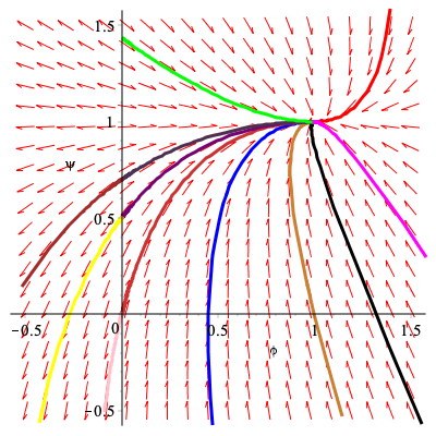
(a) $b=2$, $r=0.5,$ monostable

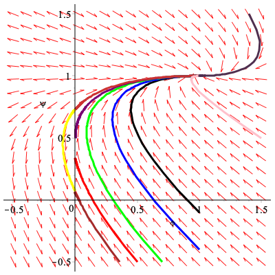
(b) $b=2$, $r=2,$ bistable cases

Figure 1: The phase plane analysis for (3) with $h=0$.

Figure 1(b) illustrates graphically the above discussion in the non-delayed case ($h=0$). Note that the lines $\phi=0$ (vertical) and $\psi=1$ (horizontal) on Figure 1 are invariant. The line $\phi=0$ consists of steady states $(0,\zeta).$ After appropriate transformations, each $\zeta\leq 1$ corresponds to the level $r(\zeta)=(1-\zeta)r$ of the bromide ion in the original system. One can ask about the existence of traveling waves connecting equilibria $(0,\zeta)$ and $(1,1)$ in (2). The homogeneous steady state $(1,1)$ is always asymptotically stable and hyperbolic, while the steady state $(0,0)$ is unstable and nonhyberbolic for $r<1$ and becomes nonhyperbolic stable for $r>1.$ Furthermore, for $r<1$ all equilibria $(0,\zeta)$, $\zeta\in(0,1)$, are unstable. For $r>1$ the equilibria $(0,\zeta)$ for $\zeta\in\left(-\infty,1-1/r\right)$ are stable and the equilibria $(0,\zeta)$ for $\zeta\in\left(1-1/r,\infty\right)$ are unstable. For the special value $\zeta_{0}=1-1/r$ we obtain $r(\zeta_{0})=1.$ The heteroclinic connections between the fixed points $(0,\zeta)$ and $(1,1)$ with $\zeta\in[\zeta_{0},1)$ are monostable, and the connections between the points $(0,\zeta)$ and $(1,1)$ with $\zeta<\zeta_{0}$ are bistable (cf. [25, p. 333]). Hence, the phase space analysis shows that with respect to the equilibria $(0,0)$ and $(1,1)$, system (2) changes its character from a monostable system to a bistable one at $r=1$ (see Figure 1).

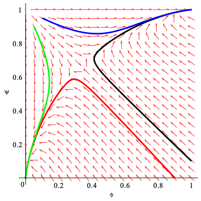
(a)

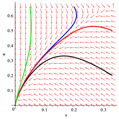
(b)

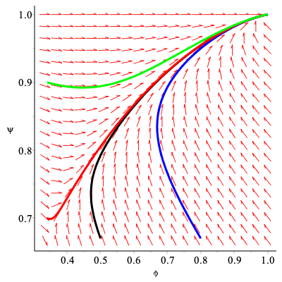
(c)

Figure 2: The phase plane analysis for (16) with $b=2$, $r=2$, $\epsilon=1$ and $h=0$: (a) the whole system, (b) and (c) two monostable subsystems.

The perturbed system (16)

(16) $$\begin{array}[]{ll}\phi^{\prime}(t)=\phi(t)(1-r-\phi(t)+r\psi(t-h)),&\\ \psi^{\prime}(t)=(b\phi(t)-\epsilon\psi(t))(1-\psi(t)),\ (\phi,\psi)\in{\mathbb{R}}^{2},&\end{array}$$

has for $h=0$ and $\epsilon>0$ two stable hyperbolic equilibria $O$ and $\beta$ and two unstable equilibria $\alpha_{1}$ and $\alpha_{2}$ of a saddle-node type, see Figure 2 (a). Consequently, system (16) is of the classical bistable type and easier to analyse. Note also that if we restrict the picture to the invariant regions $\left[0,\frac{\epsilon(r-1)}{rb-\epsilon}\right]\times\left[0,\frac{b(r-1)}{rb-\epsilon}\right]$ and $\left[\frac{\epsilon(r-1)}{rb-\epsilon},1\right]\times\left[\frac{b(r-1)}{rb-\epsilon},1\right]$ system (16) splits into two monostable subsystems, see Figure 2 (b) and (c).

Appendix B Analysis of system (16) with $r>1,\ \epsilon>0$

Recall that system (16) has exactly four equilibria

$$O=(0,0),\ \beta=(1,1),\ \alpha_{1}=(0,1),\ \alpha_{2}=\left(\frac{\epsilon(r-1)}{rb-\epsilon},\frac{b(r-1)}{rb-\epsilon}\right).$$

The right-hand side of (16) defines a continuous functional $F(\phi,\psi)$ defined on the space of continuous functions $C([-h,0],{\mathbb{R}}^{2})$. The restriction

$$F=(F_{1},F_{2}):{\mathcal{X}}_{\beta}=C([-h,0],[0,1]^{2})\to{\mathbb{R}}^{2}$$

of this functional is quasi-monotone [21, p. 78] in the sense that

$$F_{1}(\phi_{1},\psi_{1})\leq F_{1}(\phi_{2},\psi_{2}),\quad\mbox{once}\ \phi_{1}(0)=\phi_{2}(0),\ \phi_{1}(s)\leq\phi_{2}(s),\ \psi_{1}(s)\leq\psi_{2}(s).$$

$$F_{2}(\phi_{1},\psi_{1})\leq F_{2}(\phi_{2},\psi_{2}),\quad\mbox{once}\ \psi_{1}(0)=\psi_{2}(0),\ \phi_{1}(s)\leq\phi_{2}(s),\ \psi_{1}(s)\leq\psi_{2}(s).$$

By [21, Theorem 1.1, p. 78], system (16) generates a monotone semi-flow on the phase space ${\mathcal{X}}_{\beta}$. In particular, the order intervals $[O,\alpha_{2}]_{{\mathcal{X}}_{\beta}}$ and $[\alpha_{2},\beta]_{{\mathcal{X}}_{\beta}}$ are invariant.

Now, let $(\phi_{t},\psi_{t}),\ t\geq 0,$ be the solution of (16) with the initial data $(\phi_{0},\psi_{0})\in{\mathcal{X}}_{\beta}$. Suppose that $\phi_{p}(0)=0$ for some $p\geq 0$. Then from the first equation of (16) we find that $\phi_{t}(0)=0$ for all $t\geq p$. Using the second equation of the system we find that either $\psi_{t}(0)\to 0$ as $t\to+\infty$ or $\psi_{t}(0)=1,\ t\geq p$.

Similarly, if $\psi_{q}(0)=1$ for some $q\geq 0$, then from the second equation of (16) we find that $\psi_{t}(0)=1$ for all $t\geq q$. Then using the first equation of the system we find that either $\phi_{t}(0)\to 1$ as $t\to+\infty$ or $\phi_{t}(0)=0,\ t\geq q+h$.

Next, if $\phi_{p}(0)=1$ for some $p>h$, we may conclude that $\phi_{p}^{\prime}(0)=0$ and therefore $\psi_{p-h}(0)=1$. By the previous paragraph, $(\phi_{t},\psi_{t})=\beta$ for all $t\geq p$.

Finally, if $\psi_{q}(0)=0$ for some $q\geq 0$, then $\psi^{\prime}_{q}(0)=0$ and therefore, by the second equation in (16), $b\phi_{q}(0)=\epsilon\psi_{q}(0)=0$. Thus we may conclude that $(\phi_{t},\psi_{t})=O$ for all $t\geq q$.

The above analysis shows that each non-convergent solution $(\phi_{t},\psi_{t}),\ t\geq 0$, of (16) satisfies, for some $T>0$, the inequalities

$$0<\phi_{t}(0),\psi_{t}(0)<1,\quad t\geq T.$$

Let us fix some $\tau>0$ and suppose that, for some $(\phi_{0},\psi_{0})\in{\mathcal{X}}_{\beta}\setminus\{O,\alpha_{1},\alpha_{2},\beta\}$ it holds

$$(\phi_{\tau},\psi_{\tau})=(\phi_{0},\psi_{0}).$$

Thus we obtain a $\tau$-periodic solution $(\phi(t),\psi(t))=(\phi_{t}(0),\psi_{t}(0))$ with values in the open interval $(0,1)$. Clearly, this implies that

$$\int_{0}^{\tau}(1-r-\phi(s)+r\psi(s-h))ds=\int_{0}^{\tau}(b\phi(s)-\epsilon\psi(s))ds=0,$$

from where the average values $(\bar{\phi},\bar{\psi})$ of $(\phi(t),\psi(t))$ satisfy

$$(\bar{\phi},\bar{\psi})=\alpha_{2}.$$

Consequently, the elements $(\phi_{0},\psi_{0})$ and $\alpha_{2}$ are unordered in view of the monotonicity of the system. Clearly, the pair $(\phi_{0},\psi_{0})$ and $\alpha_{1}$ also cannot be ordered.

By the same reason, if for another initial data $(\phi_{0}^{*},\psi_{0}^{*})\in{\mathcal{X}}_{\beta}\setminus\{O,\alpha_{1},\alpha_{2},\beta\}$ it holds

$$(\phi^{*}_{\tau},\psi^{*}_{\tau})=(\phi^{*}_{0},\psi^{*}_{0}),$$

we obtain that

$$(\bar{\phi}^{*},\bar{\psi}^{*})=\alpha_{2}=(\bar{\phi},\bar{\psi}).$$

If the elements $(\phi_{0}^{*},\psi_{0}^{*})$ and $(\phi_{0},\psi_{0})$ were ordered, (e.g. $(\phi_{0}^{*},\psi_{0}^{*})\geq(\phi_{0},\psi_{0})$), in view of the monotonicity of the system, the inequalities

$$\phi^{*}(t)\geq\phi(t),\psi^{*}(t)\geq\psi(t),\quad t\geq 0,$$

should be satisfied. This, however, would lead to a contradiction $(\bar{\phi}^{*},\bar{\psi}^{*})>(\bar{\phi},\bar{\psi})$ since the corresponding periodic solutions are different.

Appendix C Construction of a sub-solution

Assume that $\epsilon\in(0,rb/7)$ is small enough to imply $\alpha_{21}<1/6$ and consider the following function

$$U(x)=\frac{1}{1+\rho_{1}e^{-\lambda x}}$$

with

$$\rho_{1}=\frac{r(b-\epsilon)}{\epsilon(r-1)}$$

and $\lambda$ sufficiently small, which will be specified later.

Note that $U(0)=\alpha_{21}$ and $U(x)$ satisfies the differential equations

(17) $$u^{\prime}(x)=\lambda u(x)(1-u(x)),\quad u^{\prime\prime}(x)=\lambda^{2}u(x)(1-u(x))(1-2u(x)).$$

Since $1-3U(0)>0$, for all small $\epsilon,\lambda>0$ there exists a unique point

$$x_{*}=\frac{1}{\lambda}\ln\frac{r(b-\epsilon)}{2\epsilon(r-1)}\gg 1$$

such that $1-3U(x_{*})=0$. Clearly, $1-3U(x)>0$ for all $x\in[0,x_{*})$.

Consider also $C^{3}$-smooth nonnegative function $\gamma(x)=\gamma(x,\epsilon,\lambda)$ defined as $\gamma(x)=0\ \mbox{if}\ x\leq x_{*},$ $\gamma(x)=(1-3U(x))^{4}(1-U(x))\ \mbox{if}\ x\geq x_{*}$. It is easy to find that

$$\gamma^{\prime\prime}(x)=\lambda^{2}U(x)(1-U(x))P(U(x)),\quad\gamma(x)\sim 16\rho_{1}e^{-\lambda x},\ x\to+\infty,$$

where $P$ is some real polynomial of degree 5. Let $\theta\in(0,1/16)$ be a small parameter and $V(x)$ be defined from the equation

$$1-r-U(x)+rV(x)=\theta\gamma(x).$$

Then $V(0)=\alpha_{22}$, $1-V(x)\sim\rho_{1}r^{-1}e^{-\lambda x}(1-16\theta),\ x\to+\infty,$ $V^{\prime}(x)=r^{-1}U^{\prime}(x)>0$, $x\leq x_{*}$, and, for some polynomial $Q$ of degree 4, it holds that

$$V^{\prime}(x)=r^{-1}(U^{\prime}(x)+\theta\gamma^{\prime}(x))=r^{-1}U^{\prime}(x)(1+\theta Q(U(x)))>0,\quad x\geq x_{*},$$

$$V^{\prime}(x)\leq U^{\prime}(x),\quad x\geq 0,\quad 1+\theta Q(U(x))\in[0.5,1.5],$$

for all small $\theta>0$. Therefore

$$0\leq\theta\gamma(x)=1-U(x)-r(1-V(x))\leq 1,\quad x\geq 0.$$

Next, for all $x\geq 0$ and $\lambda\in(0,\sqrt{\theta}/4)$, by using (17), we find that

$$U^{\prime\prime}(x)+U(x)(1-r-U(x)+rV(x))=$$

$$=U(x)\left(\lambda^{2}(1-2U(x))(1-U(x))+\theta\gamma(x)\right)>0.$$

Note here that $\Pi(x):=\lambda^{2}(1-2U(x))(1-U(x))+\theta\gamma(x)=\lambda^{2}(1-2U(x))(1-U(x))\geq 2\lambda^{2}/9$ for $x\in[0,x_{*}]$, $\Pi(x)=(1-U(x))(\lambda^{2}(1-2U(x))+\theta(1-3U(x))^{4})>0$ when $U(x)\in[1/3,1/2]$, and $\Pi(x)=(1-U(x))(\lambda^{2}(1-2U(x))+\theta(1-3U(x))^{4})\geq$ $(1-U(x))(\theta/16-\lambda^{2})>0$ when $U(x)\in[1/2,1)$.

Finally, for $x\in[0,x_{*}]$,

$$V^{\prime\prime}(x)+(bU(x)-\epsilon V(x))(1-V(x))=\lambda^{2}r^{-1}U(x)(1-2U(x))(1-U(x))+$$

$$r^{-1}(rb-\epsilon)\left(U(x)-\alpha_{21}\right)(1-V(x))>0,$$

as well as, for $x\geq x_{*}$, and all sufficiently small $\lambda>0$,

$$V^{\prime\prime}(x)+(bU(x)-\epsilon V(x))(1-V(x))\geq\lambda^{2}r^{-1}U(x)(1-2U(x))(1-U(x))+\theta r^{-1}\gamma^{\prime\prime}(x)+$$

$$r^{-1}(rb-\epsilon)\left(\frac{1}{3}-\alpha_{21}-\epsilon\theta(rb-\epsilon)^{-1}\gamma(x)\right)(1-V(x))>(1-U(x))\times$$

$$\left[\lambda^{2}r^{-1}U(x)\left\{1-2U(x)+\theta P(U(x))\right\}+r^{-2}\left(\frac{rb-\epsilon}{6}-\epsilon\right)(1-16\theta)\right]>0.$$

Hence, we constructed $C^{3}$- smooth functions $U(x),V(x)$ with positive derivatives on ${\mathbb{R}}_{+}$, satisfying the boundary conditions $(U,V)(0)=\alpha_{2},\ (U,V)(+\infty)=\beta$ and the inequalities

$$U^{\prime\prime}(x)+U(x)(1-r-U(x)+rV(x))>0,\ V^{\prime\prime}(x)+(bU(x)-\epsilon V(x))(1-V(x))>0,\ x\geq 0.$$

Such functions exist for all sufficiently small $\epsilon$ (an explicit upper estimate for $\epsilon$ is presented above in this appendix). Let $\eta:{\mathbb{R}}\to[0,1]$ be a smooth non-decreasing function such that $\eta(x)=0$ for all $x\leq x_{0}$, $\eta(x)=1$ for $x\geq x_{0}+1$, where we choose $x_{0}\gg 1$ such that $bU(x)-\epsilon V(x)\geq(1-V(x))br^{2}+0.5b$, $U(x)>r/(2r-1)$ for all $x\geq x_{0}$. Set

$$U(t,x)=U(x+ct)-\mu r^{2}\eta(x+ct)e^{-\delta t},\ V(t,x)=V(x+ct)-\mu\eta(x+ct)e^{-\delta t},$$

where all new parameters are positive real numbers, $\mu,\delta$ and $c$ are close to $0$. Then in the strip $0\leq x+ct\leq x_{0}$, we clearly have that

$$U_{xx}(t,x)+U(t,x)(1-r-U(t,x)+rV(t-h,x))-U_{t}(t,x)=\sigma_{1}:=$$

$$U^{\prime\prime}(x+ct)+U(x+ct)(1-r-U(x+ct)+rV(x+ct-ch))-cU^{\prime}(x+ct)>0;$$

$$V_{xx}(t,x)+(bU(t,x)-\epsilon V(t,x))(1-V(t,x))-V_{t}(t,x)=\sigma_{4}:=$$

$$V^{\prime\prime}(x+ct)+(bU(x+ct)-\epsilon V(x+ct))(1-V(x+ct))-cV^{\prime}(x+ct)>0$$

for all sufficiently small $c>0$. Let now $x+ct\geq x_{0}$. Then, for all sufficiently small positive $\mu,\delta$ and $c$,

$$U_{xx}(t,x)+U(t,x)(1-r-U(t,x)+rV(t-h,x))-U_{t}(t,x)\geq$$

$$\sigma_{1}+r^{2}\mu(\sigma_{2}+\sigma_{3}\eta(x+ct))e^{-\delta t}>0,$$

where $\sigma_{1}$ is defined above and

$$\sigma_{2}=-\eta^{\prime\prime}(x+ct)+c\eta^{\prime}(x+ct),\quad\sigma_{3}=r(1-V(x+ct))+U(x+ct)(2-r^{-1}e^{\delta h})-1-\delta+$$

$$r\mu\eta(x+ct-ch)e^{-\delta(t-h)}-\mu r^{2}\eta(x+ct)e^{-\delta t}>0.$$

Note that, for all $\xi=x+ct\geq 0$, and appropriate $\xi_{c}\in[\xi-ch,\xi]$,

$$\sigma_{1}=U^{\prime\prime}(\xi)+U(\xi)(1-r-U(\xi)+rV(\xi))+rU(\xi)(V(\xi-ch)-V(\xi))-cU^{\prime}(\xi)>$$

$$U(\xi)(\lambda^{2}(1-2U(\xi))(1-U(\xi))+$$

$$\theta\gamma(\xi)-c\lambda(1-U(\xi))-ch\lambda U(\xi_{c})(1-U(\xi_{c}))(1+\theta Q(U(\xi_{c})))>$$

$$U(\xi)\left(\lambda^{2}(1-2U(\xi))(1-U(\xi))+\theta\gamma(\xi)-(2h+1)c\lambda(1-U(\xi))\right)>0$$

if $c>0$ is small enough. Finally, if $x+ct\geq x_{0}$, then

$$V_{xx}(t,x)+(bU(t,x)-\epsilon V(t,x))(1-V(t,x))-V_{t}(t,x)=\sigma_{4}+\mu(\sigma_{2}+\sigma_{5}\eta(x+ct))e^{-\delta t}>0$$

where

$$\sigma_{5}=(bU(x+ct)-\epsilon V(x+ct))+(1-V(x+ct)+\mu\eta(x+ct)e^{-\delta t})(\epsilon-br^{2})-\delta>0.$$

Appendix D Construction of a super-solution

Let impair integer $k>r/(r-1)$ be such that $k\alpha_{22}>1$. Assume that $\epsilon\in(0,rb/2)\cap(0,1)$. For small $\lambda\in(0,\epsilon/(k+1)^{8})$, we will consider the positive increasing solution $v(x)=v(x,\lambda)$ of the boundary value problem

$$v^{\prime}(x)=\lambda v(x)(1-v(x))^{k},\ v(-\infty)=0,\ v(+\infty)=1,$$

normalised by the condition $v(0)=\alpha_{22}$. Then $v(x^{*})=1/k$ and $v(x_{*})=1/(k+1)$ for some $x_{*}<x^{*}=x^{*}(\lambda)<0$. Note that $x^{*}(\lambda)\to-\infty$ as $\lambda\to 0^{+}$,

$$v^{\prime\prime}(x)=\lambda^{2}v(x)(1-v(x))^{2k-1}(1-(k+1)v(x)).$$

The smooth function $u(x)$ will be defined from the linear equation

$$bu(x)-\epsilon v(x)=\lambda\gamma(x)\leq 0,$$

where $\gamma(x)=0$ for $x\geq x^{*}$, $\gamma(x)=-\epsilon v(x)(v(x)-1/k)^{4}=:-\epsilon P_{5}(v(x))$ for $x\leq x^{*}$. We observe that $u(0)=\alpha_{21}$ and, for the polynomial $P_{5}(v)=v(v-1/k)^{4}$ ,

$$u(x)=\frac{\epsilon}{b}\left(v(x)-\lambda P_{5}(v(x))\right),\quad u^{\prime}(x)=\frac{\epsilon}{b}v^{\prime}(x)\left(1-\lambda P_{5}^{\prime}(v(x))\right),\quad x\leq x^{*},$$

so that $u^{\prime}(x)>0$ for all $x\leq 0$ if $\lambda>0$ is sufficiently small.

Now, for $x\in[x^{*},0]$, the inequality

(18) $$v^{\prime\prime}(x)+(bu(x)-\epsilon v(x))(1-v(x))<0$$

amounts to $\lambda^{2}v(x)(1-v(x))^{2k-1}(1-(k+1)v(x))<0$ and therefore it is satisfied. On the other hand, for $x\leq x^{*}$, inequality (18) is equivalent to

$$\lambda(1-v(x))^{2(k-1)}(1-(k+1)v(x))<\epsilon\left(v(x)-\frac{1}{k}\right)^{4},$$

which is obvious for $x\in[x_{*},x^{*}]$ and also holds for $x\leq x_{*}$ since

$$\lambda(1-v(x))^{2(k-1)}(1-(k+1)v(x))<\lambda<\epsilon/(k+1)^{8}<\epsilon\left(v(x)-\frac{1}{k}\right)^{4},\ x\leq x_{*}.$$

Next, for $x\in[x^{*},0]$, the inequality

(19) $$u^{\prime\prime}(x)+u(x)(1-r-u(x)+rv(x))<0$$

holds true since, after a simplification, we find that, for $x\in[x^{*},0]$,

$$\lambda^{2}(1-v(x))^{2k-1}(1-(k+1)v(x))+1-r+(r-\epsilon/b)v(x)\leq$$

$$\lambda^{2}(1-v(x))^{2k-1}(1-(k+1)v(x))+1-r+(r-\epsilon/b)v(0)=$$

$$\lambda^{2}(1-v(x))^{2k-1}(1-(k+1)v(x))<0.$$

If we take $x\leq x^{*}$, then (19) is true because, for all sufficiently small $\lambda>0$ and some real polynomial $P_{2k+4}(v)$ of degree $2k+4$, it holds

$$v^{\prime\prime}(x)+v(x)(1-r+(r-\epsilon/b)v(x))+$$

$$\lambda\left[-P_{5}(v(x))^{\prime\prime}-P_{5}(v(x))\left(1-r+\left(r-\frac{2\epsilon}{b}\right)v(x)+\frac{\lambda\epsilon}{b}P_{5}(v(x))\right)\right]<$$

$$v(x)(1-r+\frac{r-\epsilon/b}{k}+\lambda^{2})+\lambda\left[-P_{5}(v(x))^{\prime\prime}-P_{5}(v(x))\left(1-r\right)\right]<$$

$$v(x)\left(1-r+\frac{r-\epsilon/b}{k}+\lambda^{2}+\lambda\left[\lambda^{2}P_{2k+4}(v(x))+\frac{r-1}{k^{4}}\right]\right)<0.$$

Finally, let $\eta:{\mathbb{R}}\to[0,1]$ be a smooth non-decreasing function such that $\eta(x)=0$ for all $x\geq x_{0}$, $\eta(x)=1$ for $x\leq x_{0}-1$, where we choose $x_{0}\ll x_{*}$. Set

$$U(t,x)=u(x)+\mu(\epsilon/3b)\eta(x)e^{-\delta t},\ V(t,x)=v(x)+\mu\eta(x)e^{-\delta t},$$

where all new parameters are positive real numbers, $\mu$ is close to $0$. Then in the strip $x_{0}\leq x\leq 0$, we have that $U(t,x)=u(x),\ V(t,x)=v(x)$ and therefore

$$\mathcal{D}_{1}(U,V):=U_{xx}(t,x)+U(t,x)(1-r-U(t,x)+rV(t-h,x))-U_{t}(t,x)<0,$$

$$\mathcal{D}_{2}(U,V):=V_{xx}(t,x)+(bU(t,x)-\epsilon V(t,x))(1-V(t,x))-V_{t}(t,x)<0.$$

Now, if $x\leq x_{0}$, then for all sufficiently small $\mu>0$, $\delta>0$,

$$\mathcal{D}_{1}(U,V)=\mathcal{D}_{1}(u,v)+\mathcal{D}_{1}(\mu(\epsilon/3b)\eta(x)e^{-\delta t},\mu\eta(x)e^{-\delta t})+$$

$$\mu\eta(x)u(x)e^{-\delta t}(-2\epsilon/3b+re^{\delta h})+\mu(r\epsilon/3b)\eta(x)e^{-\delta t}v(x)<0,$$

$$\mathcal{D}_{2}(U,V)=v^{\prime\prime}(x)+\mu\eta^{\prime\prime}(x)e^{-\delta t}+(\lambda\gamma(x)-(2/3)\epsilon\mu\eta(x)e^{-\delta t})(1-v(x)-\mu\eta(x)e^{-\delta t})+$$

$$\mu\delta\eta(x)e^{-\delta t}<v^{\prime\prime}(x)+\lambda\gamma(x)(1-v(x))+$$

$$\mu e^{-\delta t}\left[\eta^{\prime\prime}(x)-\eta(x)\epsilon\left\{\frac{2}{3}\left(1-\frac{1}{k+1}-\mu\right)-\frac{\lambda}{k^{5}}\right\}+\delta\eta(x)\right]<0.$$

References

- [1] A. Boumenir and V. M. Nguyen, Perron theorem in the monotone iteration method for traveling waves in delayed reaction-diffusion, J. Differ. Equ., 244 (2008), pp. 1551–1570, https://doi.org/10.1016/j.jde.2008.01.004.
- [2] M. Bramson, Convergence of solutions of the Kolmogorov equation of travelling waves, Memoirs of the American Mathematical Society, 44 (1983).
- [3] Z. Du and Q. Qiao, The dynamics of traveling waves for a nonlinear Belousov-Zhabotinskii system, J. Differ. Equ., 269 (2020), pp. 7214–7230, https://doi.org/10.1016/j.jde.2020.05.033.
- [4] J. Fang and X.-Q. Zhao, Bistable traveling waves for monotone semiflows with applications, J. Eur. Math. Soc., 17 (2015), pp. 2243–2288, https://doi.org/10.4171/JEMS/556.
- [5] P. C. Fife and M. M. Tang, Comparison principles for reaction-diffusion systems: Irregular comparison functions and applications to questions of stability and speed of propagation of disturbances, J. Differ. Equ., 40 (1981), pp. 168–185, https://doi.org/10.1016/0022-0396(81)90016-4.
- [6] R. G. Gibbs, Travelling waves in the Belousov-Zhabotinski reaction, SIAM J. Appl. Math., 38 (1980), pp. 422–444, https://doi.org/10.1137/0138035.
- [7] J. K. Hale and Sjoerd M. Verduyn Lunel, Introduction to Functional Differential Equations, Springer, New York, NY, 1st ed., 1993, https://doi.org/10.1007/978-1-4612-4342-7.
- [8] B.-S. Han, M.-X. Chang, and W.-J. Bo, Traveling waves for a Belousov–Zhabotinsky reaction–diffusion system with nonlocal effect, Nonlinear Analysis: Real World Applications, 64 (2022), p. 103423, https://doi.org/https://doi.org/10.1016/j.nonrwa.2021.103423.
- [9] K. Hasík, J. Kopfová, P. Nábělková, O. Trofymchuk, and S. Trofimchuk, Two reasons for the appearance of pushed wavefronts in the Belousov-Zhabotinsky system with spatiotemporal interaction, June 2022, https://doi.org/10.48550/arXiv.2206.03613.
- [10] D. Henry, Geometric theory of semilinear parabolic equations, Springer-Verlag, Berlin Heidelberg, 1st ed., 1981.
- [11] Y.-I. Kanel, Existence of a traveling-wave type solutions for the Belousov-Zhabotinskii system of equations ii, Sib. Math. J., 32 (1991), pp. 390–400, https://doi.org/10.1007/BF00970474.
- [12] S. Ma, Traveling wavefronts for delayed reaction-diffusion systems via a fixed point theorem, J. Differ. Equ., 171 (2001), pp. 294–314, https://doi.org/10.1006jdeq.2000.3846.
- [13] V. Manoranjan and A. Mitchell, A numerical study of the Belousov-Zhabotinskii reaction using galerkin finite element methods, J. Math. Biology, 16 (1983), p. 251–260, https://doi.org/10.1007/BF00276505.
- [14] R. H. Martin and H. L. Smith, Abstract functional differential equations and reaction-diffusion systems, Trans. Amer. Math. Soc., 321 (1990), pp. 1–44, https://doi.org/10.2307/2001590.
- [15] J. D. Murray, On traveling wave solutions in a model for Belousov-Zhabotinskii reaction, Journal of Theoretical Biology, 56 (1976), pp. 329–353, https://doi.org/10.1016/S0022-5193(76)80078-1.
- [16] J. D. Murray, Lectures on nonlinear differential equations. Models in biology, Clarendon Press, Oxford, 1st ed., 1977.
- [17] J. D. Murray, Mathematical Biology, Vol. 1, Springer-Verlag, Berlin, 3rd ed., 2002.
- [18] H.-T. Niu, Z.-C. Wang, and Z.-H. Bu, Curved fronts in the Belousov–Zhabotinskii reaction–diffusion systems in , Journal of Differential Equations, 264 (2018), pp. 5758–5801, https://doi.org/https://doi.org/10.1016/j.jde.2018.01.020.
- [19] D. A. Quinney, On computing travelling wave solutions in a model for the Belousov-Zhabotinskii reaction, IMA Journal of Applied Mathematics, 23 (1979), pp. 193–201, https://doi.org/10.1093/imamat/23.2.193.
- [20] H. Smith and X.-Q. Zhao, Global asymptotic stability of traveling waves in delayed reaction-diffusion equations, SIAM Journal Math. Anal., 31 (2000), pp. 514–534, https://doi.org/10.1137/S0036141098346785.
- [21] H. L. Smith, Monotone dynamical systems, Amer. Math. Soc., Providence, 1st ed., 1995.
- [22] E. Trofimchuk, M. Pinto, and S. Trofimchuk, Traveling waves for a model of the Belousov-Zhabotinsky reaction, J. Differ. Equ., 254 (2013), pp. 3690–3714, https://doi.org/10.1016/j.jde.2013.02.005.
- [23] E. Trofimchuk, M. Pinto, and S. Trofimchuk, On the minimal speed of front propagation in a model of the Belousov- Zhabotinsky reaction, Discrete Contin. Dyn. Syst. Ser. B, 19 (2014), pp. 1769–1781, https://doi.org/10.3934/dcdsb.2014.19.1769.
- [24] W. C. Troy, The existence of traveling wave front solutions of a model of the Belousov-Zhabotinskii reaction, Journal of Differential Equations, 36 (1980), pp. 89–98, https://doi.org/10.1016/0022-0396(80)90078-9.
- [25] A. Volpert, V. A. Volpert, and V. A. Volpert, Traveling Wave Solutions of Parabolic Systems, Amer. Math. Soc., Providence, 1st ed., 1994.
- [26] V. Volpert, Existence of waves for a bistable reaction–diffusion system with delay, Journal of Dynamics and Differential Equations, 32 (2020), pp. 615–629, https://doi.org/10.1007/s10884-019-09751-4.
- [27] L. Wang, Y. Zhao, and Y. Wu, The stability of traveling wave fronts for Belousov-Zhabotinskii system with small delay, Discrete Contin. Dyn. Syst. Ser. B, 28 (2023), pp. 3887–3897, https://doi.org/10.3934/dcdsb.2022246.
- [28] J. Wu and X. Zou, Traveling wave fronts of reaction-diffusion systems with delay, Journal of Dynamics and Differential Equations, 13 (2001), pp. 651–687, https://doi.org/10.1023/A:1016690424892.
- [29] G. B. Zhang, Asymptotics and uniqueness of traveling wavefronts for a delayed model of the Belousov-Zhabotinsky reaction, Applicable Analysis, 99 (2020), pp. 1639–1660, https://doi.org/10.1080/00036811.2018.1542686.