Finite flocking time of the nonlinear Cucker–Smale model with Rayleigh friction type using the discrete $p$-Laplacian

Abstract

The study of collective behavior in multi-agent systems has attracted the attention of many researchers due to its wide range of applications. Among them, the Cucker-Smale model was developed to study the phenomenon of flocking, and various types of extended models have been actively proposed and studied in recent decades.

In this study, we address open questions of the Cucker–Smale model with norm-type Rayleigh friction: (i) The positivity of the communication weight, (ii) The convergence of the norm of the velocities of agents, (iii) The direction of the velocities of agents. For problems (i) and (ii), we present the nonlinear Cucker–Smale model with norm-type Rayleigh friction, where the nonlinear Cucker–Smale model is generalized to a nonlinear model by applying a discrete $p$-Laplacian operator. For this model, we present conditions that guarantee that the norm for velocities of agents converges to 0 or a positive value, and we also show that the regular communication weight satisfies the conditions given in this study. In particular, we present a condition for the initial configuration to obtain that the norm of agent velocities converges to only some positive value.

By contrast, problem (iii) is not solved by the norm-type nonlinear model. Thus, we propose a nonlinear Cucker–Smale model with a vector-type Rayleigh friction for problem (iii). In parallel to the first model, we show that the direction of the agents’ velocities can be controlled by parameters in the nonlinear Cucker–Smale model with the vector-type Rayleigh friction.

1 Introduction

In recent years, there has been a growing interest among researchers in the development and analysis of mathematical models for multi-agent systems (MAS) in fields including biology, social sciences, physics, and engineering. The modeling of MAS as a system of mathematical differential equations has emerged as an active research area, providing a powerful tool for comprehending complex phenomena such as the flocking of birds, schooling of fish, and colonization of bacteria. This improved understanding can also facilitate the development of more efficient engineering systems, including unmanned aerial vehicles. Consequently, various models, such as the Vicsek model, Kuramoto model, minimal model, and Cucker–Smale model, have been proposed and are being studied in different fields (see [2, 3, 19, 20, 21, 24] and the references therein).

In this study, we are interested in the Cucker–Smale model with Rayleigh friction. The Cucker–Smale model (C-S model) was first introduced in [12] to study the collective and self-driven motion of self-propelled agents. The mathematical model is given by

$$\frac{dx_{i,k}}{dt}(t)=v_{i,k}(t),$$

$$\frac{dv_{i,k}}{dt}(t)=\sum_{j=1}^{N}\psi_{R}(\|x_{j}(t)-x_{i}(t)\|_{2}^{2})(v_{j,k}(t)-v_{i,k}(t)),\quad i\in\mathcal{I}:=\{1,\ldots,N\},~{}k\in\mathcal{K}:=\{1,\ldots,d\},$$

where $N$ is the number of agents, $a$ is a positive coupling strength, $x_{i}=(x_{i,1},\ldots x_{i,d})\in\mathbb{R}^{d}$, and $v_{i}=(v_{i,1},\ldots v_{i,d})\in\mathbb{R}^{d}$ are the position and velocity of the $i$th agent in phase space $\mathbb{R}^{d}\times\mathbb{R}^{d}$, respectively, $\psi_{R}$ is a regular communication weight defined by $\psi_{R}(s)=\frac{K}{\left(1+s\right)^{\beta}}$ for some $\beta>0$ and $K>0$, and $\|\cdot\|_{2}$ is the Euclidean norm. For this model, Cucker and Smale presented conditions to ensure that agents’ velocities converge to a common velocity and that the maximum distance between agents is uniformly bounded, i.e., the so-called “asymptotic flocking” is defined by

• The relative velocity fluctuations tend to zero as time tends to infinity (velocity alignment, or consensus):

  $$\lim_{t\to\infty}\left\|v_{j}(t)-v_{i}(t)\right\|_{2}=0,\text{ for all }i,j\in\mathcal{I},$$

• The diameter of a group is uniformly bounded in time t (forming a group):

  $$\sup_{t\geq 0}\left\|x_{j}(t)-x_{i}(t)\right\|_{2}<\infty\text{ for all }i,j\in\mathcal{I}.$$

This C-S model was later extended into various forms depending on the purpose of each study, such as, (mono-cluster) flocking [12, 16, 17, 22], multi-cluster flocking [9, 8], pattern formation [10, 23], collision-avoidance [1, 6, 7, 11], leadership [13, 14, 25], and forcing terms and control [4, 15].

In particular, among these models, the C-S model with Rayleigh friction [15] caught our attention. In [15], Ha and his colleagues introduced the C-S model with Rayleigh friction:

$$\frac{dx_{i,k}}{dt}(t)=v_{i,k}(t),$$ (1)

$$\frac{dv_{i,k}}{dt}(t)=\frac{\lambda}{N}\sum_{j=1}^{N}\psi(\|x_{j}(t)-x_{i}(t)\|_{2}^{2})(v_{j,k}(t)-v_{i,k}(t))+\delta v_{i,k}(1-\left\|v_{i}(t)\right\|_{2}^{2}),$$ (2)

for $i\in\mathcal{I}$, $k\in\mathcal{K}$, $\lambda>0$, $\delta>0$, and $\psi:\mathbb{R}\to\mathbb{R}$ is a communication weight function satisfying

$$\psi(s)\geq\psi_{*}>0,\quad\text{for some positive constant }\psi_{*}$$ (3)

to investigate how Rayleigh-type friction affects the dynamics of the C-S system. They proved that if $\lambda\psi_{*}>\delta$, the system (1)-(2) induces the flocking behavior of agents. Moreover, the norm of velocities converges to 0 or 1, that is, $\left\|v_{i}(t)\right\|_{2}\to 0\text{ or }1$ as $t\to\infty$ for all $i\in\mathcal{I}$.

In particular, we note that some open problems have been discussed in [15]:

• (Problem for the condition $\psi(s)\geq\psi_{*}>0$, $s\in\mathbb{R}$) Since they assumed $\psi(s)\geq\psi_{*}>0$, $s\in\mathbb{R}$, their results cannot be applied for the algebraically decaying communication C-S weight with $\psi_{*}=0$, such as the regular communication weight $\psi_{R}$. Therefore, we must determine a condition weaker than condition (3).

• (Problem for the convergence of $\left\|v_{i}\right\|_{2}$) For this problem, they assumed that it is not apriori clear which initial configuration converges to 0 or 1.

• (Problem for the direction of velocity) From the results in [15], we only know the convergence of agents’ speed (i.e., $\left\|v_{i}\right\|_{2}$), not their velocities.

The aim of this paper was to address these open problems using a nonlinear operator called the discrete $p$-Laplacian defined by

$$\Delta_{p,\psi}v_{i,k}=\sum_{j=1}^{N}\psi\left(\|x_{j}-x_{i}\|_{2}\right)|v_{j,k}-v_{i,k}|^{p-2}(v_{j,k}-v_{i,k}),$$

where $p>1$, and $\psi:[0,\infty)\to[0,\infty)$ is a non-increasing and differentiable function. We applied the discrete $p$-Laplacian because of its properties. To the best of our knowledge, the discrete Laplacian (that is, $p=2$) only provides information about the asymptotic behavior of the agents owing to technical reasons. For example, the norm of $v_{i}$ decays exponentially; however, we do not know whether $\left\|v_{i}\right\|_{2}=0$ in finite time. Furthermore, if $1<p<2$, due to the discrete $p$-Laplacian, agents’ behavioral properties, such as flocking and consensus, can be revealed in finite time (see [18]). We intend to use these features to address the open problems mentioned above. Therefore, we consider a nonlinear C-S model with (norm-type) Rayleigh friction applying the discrete $p$-Laplacian:

$$\frac{dx_{i,k}}{dt}=v_{i,k}$$ (4)

$$\frac{dv_{i,k}}{dt}=\Delta_{p,\psi}v_{i,k}+av_{i,k}\left\|v_{i}\right\|_{2}^{q-2}-bv_{i,k}\left\|v_{i}\right\|_{2}^{r-2},$$ (5)

where $p>1$, $q>1$, $r>1$, $a>0$, $b>0$, and $x_{i}=(x_{i,1},\ldots,x_{i,d})$ and $v_{i}=(v_{i,1},\ldots,v_{i,d})$ are the position and velocity of $i$-th particle in $\mathbb{R}^{d}$, respectively. Here, for $p=2$, $q=2$, $r=4$, and $a=b=\delta$, the system (4)-(5) implies the C-S model with Rayleigh friction (1)-(2).

For the model (4)-(5) in this study, we first show that if $p>1$, $2\leq q<r$, and the initial configuration for the agents’ velocities is non-negative and non-zero, then the system (4)-(5) forms an asymptotic flocking and the velocities satisfy $\lim_{t\to\infty}\left\|v_{i}(t)\right\|_{2}=\left(\frac{a}{b}\right)^{\frac{1}{r-q}}$. We present a condition to guarantee that the system (4)-(5) has a finite flocking time and the velocities satisfy $\lim_{t\to\infty}\left\|v_{i}(t)\right\|_{2}=\left(\frac{a}{b}\right)^{\frac{1}{r-q}}$ or $0$ for $1<p<2\leq q<r$, $a>0$, and an arbitrary initial configuration. The given condition is as follows:

$$4C_{m}\left(1-\frac{p}{2}\right)\int_{0}^{\infty}\min_{i,j\in\mathcal{I}}\psi(\|x_{j}(t)–x_{i}(t)\|_{2})dt>\left(\sum_{k\in\mathcal{K}}\left(\max_{i\in\mathcal{I}}v_{i,k}(0)-\min_{i\in\mathcal{I}}v_{m,k}(0)\right)^{2}\right)^{\frac{2-p}{2}}$$ (6)

where $C_{m}$ is positive and defined in Section 2, and the finite flocking time indicates that there exists a positive time $T>0$ such that $\left\|v_{j}(t)-v_{i}(t)\right\|_{2}=0$, for all $i,j\in\mathcal{I}$, and $t\geq T$.

In particular, we note that the condition (6) is weaker than (3) presented in [15] and the regular communication weight $\psi_{R}$ satisfies (6), which is proved in Section 5. This expression solves problem one (P1). Moreover, the existence of the finite flocking time provides a condition for the initial (velocity) configuration to solve problem two (P2); that is, from the presented condition, $\left\|v_{i}(t)\right\|_{2}$ converges to only $\left(\frac{a}{b}\right)^{\frac{1}{r-q}}$ as $t\to\infty$. However, we, unfortunately, do not obtain any information about the direction of the agents’ progress (i.e., velocities of agents) for the nonlinear C-S model with (norm-type) Rayleigh friction. The reason for this is that (5) contains the norm term $\left\|\cdot\right\|_{2}$; hence, we can only obtain information about $\left\|v_{i}\right\|_{2}$ and not each velocity $v_{i,k}$, $k\in\mathcal{K}$ due to the limitations of technical methods of solving ordinary differential equations.

Therefore, for the open problem (P3), we propose the nonlinear C-S model with (vector-type) Rayleigh friction:

$$\frac{dx_{i,k}}{dt}=v_{i,k}$$ (7)

$$\frac{dv_{i,k}}{dt}=\Delta_{p,\psi}v_{i,k}+a_{k}\varphi_{q}(v_{i,k})-b_{k}\varphi_{r}(v_{i,k})$$ (8)

where $a_{k}>0$, $b_{k}>0$ for $k\in\mathcal{K}$, and the function $\varphi_{\gamma}$ is defined by $\varphi_{\gamma}(s):=|s|^{\gamma-2}s$, $s\in\mathbb{R}$, $\gamma>1$, to control the direction of the agents’ progress. For this model, we show that for $1<p<2$, $p<q<r$, and $k\in\mathcal{K}$, if the initial velocity configuration is non-negative and non-zero, $\lim_{t\to\infty}v_{i,k}(t)=\left(\frac{a_{k}}{b_{k}}\right)^{\frac{1}{r-q}}$ for all $i\in\mathcal{I}$ and the system (7)-(8) forms asymptotic flocking. We also present conditions for the initial configuration to guarantee the existence of finite flocking time, using which, we can see that $v_{i,k}$ converges to either $\left(\frac{a_{k}}{b_{k}}\right)^{\frac{1}{r-q}}$, $0$, or $-\left(\frac{a_{k}}{b_{k}}\right)^{\frac{1}{r-q}}$. Finally, we present a condition for the initial velocity configuration to guarantee that $v_{i,k}$ converges to only $\left(\frac{a_{k}}{b_{k}}\right)^{\frac{1}{r-q}}$. We note that as shown in the system (7)-(8) above, the difference from systems (4)-(5) is that the vector type term $\varphi_{\gamma}$ is given instead of the norm type term. This is a very simple change. However, it will allow us to obtain microscopic information about the velocity $v_{i,k}$ of each agent using the maxima and minima of $v_{i,k}$, rather than macroscopic information such as the norm.

The remainder of this paper is organized as follows. Section 2 introduces the preliminary concepts and useful well-known results. Section 3 is devoted to a discussion of the nonlinear C-S model with a norm-type Rayleigh friction, and in Section 4, we address the nonlinear C-S model with the vector-type Rayleigh friction. In Section 5, we show that the regular communication weight satisfies the conditions presented in Sections 3 and 4. Finally, we provide several numerical simulations to confirm our analytical results.

2 Preliminaries

We start this section with maximum and minimum functions defined by $v_{M,k}(t):=\max_{i\in\mathcal{I}}v_{ik}(t)$ and $v_{m,k}(t):=\min_{i\in\mathcal{I}}v_{ik}(t)$ for $k\in\mathcal{K}$ and $t\geq 0$. Let us define two index sets: for each $t\geq 0$ and $k\in\mathcal{K}$,

$$\mathcal{I}_{M,k}^{t}:=\{i\in\mathcal{I}~{}|~{}v_{M,k}(t)=v_{i,k}(t)\}\text{ and }\mathcal{I}_{m,k}^{t}:=\{i\in\mathcal{I}~{}|~{}v_{m,k}(t)=v_{i,k}(t)\}.$$

Since $\Delta_{p,\psi}v_{M,k}(t)\leq 0$ and $\Delta_{p,\psi}v_{m,k}(t)\geq 0$ for all $k\in\mathcal{K}$ and $t\geq 0$, for $i\in\mathcal{I}_{M,k}^{t}$ and $j\in\mathcal{I}_{m,k}^{t}$,

$$v_{i,k}^{\prime}= \Delta_{p,\psi}v_{M,k}+av_{i,k}f(v_{i})-bv_{i,k}g(v_{i})$$

$$\leq bv_{i,k}f(v_{i})\left(\frac{a}{b}-\frac{g(v_{i})}{f(v_{i})}\right),$$

and

$$v_{j,k}^{\prime}= \Delta_{p,\psi}v_{m,k}+av_{j,k}f(v_{j})-bv_{j,k}g(v_{j})$$

$$\geq bv_{j,k}f(v_{j})\left(\frac{a}{b}-\frac{g(v_{j})}{f(v_{j})}\right),$$

where $f$ and $g$ are specified by norm-type as in (5) or vector-type as in (8) in accordance with the theme of each section. Since we always assume that $q<r$, $\frac{g(v)}{f(v)}$ is well-defined for $v\in\mathbb{R}$ and strictly increases and decreases on $(0,\infty)$ and $(-\infty,0)$, respectively. Thus, if $v_{i,k}(t)$ is large enough on some time interval $I$ such that $\frac{g(v_{i})}{f(v_{i})}>\frac{a}{b}$, then $v_{i,k}$ strictly decreases on the interval $I$. By contrast, if $v_{j,k}$ is small enough on some interval $I$ such that $\frac{g(v_{j})}{f(v_{j})}>\frac{a}{b}$, then $v_{j,k}$ strictly increases on the interval $I$. Therefore, $v_{i,k}$ is uniformly bounded with respect to $t\geq 0$ for all $i\in\mathcal{I}$, $k\in\mathcal{K}$. Using (5) and (8), $v_{i,k}^{\prime}$ is also uniformly bounded. Hence, $v_{i,k}$ is Lipschitz continuous, and $v_{M,k}$ and $v_{m,k}$ are also Lipschitz continuous. Therefore, $v_{M,k}$ and $v_{m,k}$ are differentiable almost everywhere.

Throughout this paper, we assume that for each $k\in\mathcal{K}$, there exist distinct time series $\{t_{l}\}_{l=0}^{\infty}$ and $\{s_{l}\}_{l=0}^{\infty}$ such that the indices $M$ and $m$ do not change on $(s_{l},s_{l+1})$ and $(t_{l},t_{l+1})$, respectively. Then, it is clear that $v_{M,k}\in C^{1}((s_{l-1},s_{l}))$ and $v_{m,k}\in C^{1}((t_{l-1},t_{l}))$ where $C^{1}((a,b))$ is a class consisting of all differentiable functions whose derivative is continuous on $(a,b)$. Moreover, since $v_{i,k}$ is continuous with respect to $t$,

$$\int_{a}^{b}v_{M,k}^{\prime}(s)ds=v_{M,k}(b)-v_{M,k}(a),\quad\text{and}\quad\int_{a}^{b}v_{m,k}^{\prime}(s)ds=v_{m,k}(b)-v_{m,k}(a).$$

We note that $v_{M,k}$ and $v_{m,k}$ may or may not be differentiable at $t=s_{l}$ and $t=t_{l}$. However, since there always exist $i\in\mathcal{I}_{M,k}^{s_{l}}$ and $j\in\mathcal{I}_{m,k}^{t_{l}}$ such that $v_{M,k}(s_{l})=v_{i,k}(s_{l})$ and $v_{m,k}(t_{l})=v_{j,k}(t_{l})$, we consider $v_{M,k}^{\prime}(s_{l})<\alpha$ and $v_{m,k}^{\prime}(t_{l})<\alpha$ for some $\alpha\in\mathbb{R}$ as $v_{i,k}^{\prime}(s_{l})<\alpha$ and $v_{j,k}^{\prime}(t_{l})<\alpha$ for all $i\in\mathcal{I}_{M,k}^{t}$ and $j\in\mathcal{I}_{m,k}^{t}$. The same considerations apply to other inequalities ($>$, $\geq$ and $\leq$). In addition, if necessary, we consider the derivatives of $v_{M,k}$ and $v_{m,k}$ at $t=s_{l}$ and $t=t_{l}$, respectively, as

$$v_{M,k}^{\prime}(s_{l})=\lim_{t\to s_{l}^{+}}v_{i,k}^{\prime}(t),\quad v_{m,k}^{\prime}(t_{l})=\lim_{t\to t_{l}^{+}}v_{j,k}^{\prime}(t)$$

for some $i\in\{i\in\mathcal{I}~{}|~{}v_{M,k}(t)=v_{i,k}(t),~{}t\in(s_{l},s_{l+1})\}$ and $j\in\{i\in\mathcal{I}~{}|~{}v_{m,k}(t)=v_{i,k}(t),~{}t\in(t_{l},t_{l+1})\}$.

We now recall some well-known properties for the $p$-norm $\left\|\cdot\right\|_{p}$ without proofs, defined by $\left\|\mathbf{a}\right\|_{p}:=\sum_{i\in\mathcal{I}}a_{i}$ if $\mathbf{a}=(a_{1},\ldots,a_{N})$ is a vector in $\mathbb{R}^{N}$, and $\left\|\mathbf{a}\right\|_{\gamma}:=\left(\sum_{i\in\mathcal{I}}\sum_{k\in\mathcal{K}}a_{i,k}^{\gamma}\right)^{\frac{1}{\gamma}}$ if $\mathbf{a}=(a_{i,k})_{N\times d}$ is a $N\times d$-matrix. These properties are useful when dealing with norms in this study.

Lemma 2.1 ([5]).

For $\gamma>1$, $d\geq 1$, and $\delta\geq 0$, there exist $C_{1}(p,d)>0$ and $C_{2}(p,d)>0$ such that for all $x,y\in\mathbb{R}^{d}$,

$$\left\|\left\|x\right\|_{2}^{\gamma-2}x-\left\|y\right\|_{2}^{\gamma-2}y\right\|_{2}\leq C_{1}\left\|x-y\right\|_{2}^{1-\delta}\left(\left\|x\right\|_{2}+\left\|y\right\|_{2}\right)^{\gamma-2+\delta},$$ (9)

and

$$\Big{\langle}x-y,\left\|x\right\|_{2}^{\gamma-2}x-\left\|y\right\|_{2}^{\gamma-2}y\Big{\rangle}\geq C_{2}\left\|x-y\right\|_{2}^{2+\delta}\left(\left\|x\right\|_{2}+\left\|y\right\|_{2}\right)^{\gamma-2-\delta},$$ (10)

where $\Big{\langle}\cdot,\cdot\Big{\rangle}$ is the dot product, and $\left\|\cdot\right\|_{2}$ is the Euclidean norm.

Proof.

For a proof of this lemma, see [5, Lemma 2.2]. ∎

Lemma 2.2.

For any vector $\mathbf{a}_{i}=(a_{i1},\ldots,a_{id})\in\mathbb{R}^{d}$, $i=1,\ldots,N$, if $1<r\leq s$, then

$$\|\mathbf{a}\|_{s}\leq\|\mathbf{a}\|_{r}\leq(Nd)^{\frac{1}{r}-\frac{1}{s}}\|\mathbf{a}\|_{s},$$

where $\mathbf{a}=(a_{ik})\in\mathbb{R}^{N\times d}$ is a $N\times d$ matrix whose elements are given by $a_{ik}$, and $\left\|\mathbf{a}\right\|_{\gamma}:=\left(\sum_{i\in\mathcal{I}}\sum_{k\in\mathcal{K}}a_{ik}^{\gamma}\right)^{\frac{1}{\gamma}}$.

Proof.

This lemma is very well-known. Therefore, we omit its proof, which can be obtained from [18, Appendix C]. ∎

Remark 2.3.

By Lemma 2.2, it is clear that

$$C_{m}\|\mathbf{a}\|_{s}\leq\|\mathbf{a}\|_{r}\leq C_{M}\|\mathbf{a}\|_{s}$$ (11)

for any $r>1$, $s>1$, and $\mathbf{a}\in\mathbb{R}^{N\times d}$. Here, $C_{M}$ and $C_{m}$ are defined by

$$C_{M}:=\max\left\{1,(Nd)^{\frac{1}{r}-\frac{1}{s}}\right\},\quad\text{ and }\quad C_{m}:=\min\left\{1,(Nd)^{\frac{1}{r}-\frac{1}{s}}\right\}.$$

3 Norm type Rayleigh friction

In this section, we discuss problems P1 and P2 by analyzing the nonlinear C-S model with norm-type Rayleigh friction:

$$\frac{dx_{ik}}{dt}=v_{ik}$$ (12)

$$\frac{dv_{ik}}{dt}=\Delta_{p,\psi}v_{ik}+av_{ik}\left\|v_{i}\right\|_{2}^{q-2}-bv_{ik}\left\|v_{i}\right\|_{2}^{r-2},$$ (13)

where $p>1$. In particular, we assume that $2\leq q<r$ to ensure that $\left\|\cdot\right\|_{2}^{q-2}$ and $\left\|\cdot\right\|_{2}^{r-2}$ are well-defined. By the definitions of $v_{M,k}$ and $v_{m,k}$, (13) implies that for each $k\in\mathcal{K}$,

$$v_{M,k}^{\prime}\leq bv_{M,k}\left\|v_{M}\right\|_{2}^{q-2}\left(\frac{a}{b}-\left\|v_{M}\right\|_{2}^{r-q}\right),$$

and

$$v_{m,k}^{\prime}\geq bv_{m,k}\left\|v_{m}\right\|_{2}^{q-2}\left(\frac{a}{b}-\left\|v_{m}\right\|_{2}^{r-q}\right).$$

Thus, for a fixed $k\in\mathcal{K}$, if $v_{M,k}(t)>\left(\frac{a}{b}\right)^{\frac{1}{r-q}}$ on some time interval $I$, then $v_{M,k}$ is strictly decreasing on the interval $I$, and if $v_{m,k}(t)<-\left(\frac{a}{b}\right)^{\frac{1}{r-q}}$ on some interval $I$, then $v_{m,k}(t)$ is strictly increasing on the interval $I$. These properties indicate that for each $i\in\mathcal{I}$ and $k\in\mathcal{K}$, $v_{i,k}$ is uniformly bounded with respect to $t$ by

$$\min\left\{-\left(\frac{a}{b}\right)^{\frac{1}{r-q}},v_{m,k}(0)\right\}\leq v_{i,k}(t)\leq\max\left\{\left(\frac{a}{b}\right)^{\frac{1}{r-q}},v_{M,k}(0)\right\},\quad t\geq 0.$$

Therefore, we have $|v_{i,k}(t)|\leq\max\left\{\left(\frac{a}{b}\right)^{\frac{1}{r-q}},\max_{i\in\mathcal{I},k\in\mathcal{K}}|v_{i,k}(0)|\right\}$ for all $i\in\mathcal{I}$, $k\in\mathcal{K}$, and $t\geq 0$.

We now discuss more detailed properties of $v_{i,k}$ under a non-negative (or non-positive) and non-zero initial velocity configuration.

Lemma 3.1.

If there exist $T\geq 0$ and $k\in\mathcal{K}$ such that $v_{i,k}(T)$ is non-negative and non-zero (that is, $v_{i,k}(T)\not\equiv 0$ with respect to $i$), then we have either

$$v_{m,k}(t)>0,\quad t>T,$$

or there exists $T^{\prime}>T$ such that

$$v_{m,k}(t)>0,~{}t\in(T,T^{\prime}),\quad\text{ and }\quad v_{M,k}(t)=v_{m,k}(t)=0,~{}t\in[T^{\prime},\infty),$$

Proof.

For the given $k\in\mathcal{K}$, we first assume $v_{m,k}(T)=0$. Since $v_{i,k}$ is non-zero at $t=T$, we have $0=v_{m,k}(T)<v_{M,k}(T)$, implying that $v_{m,k}^{\prime}(T)=\Delta_{p,\psi}v_{m,k}(T)>0$. Hence, there exists $\delta>0$ such that $v_{m,k}(T+\delta)>0$. Consequently, without loss of generality, we may assume that $v_{m,k}(T)>0$. If there exists a minimum $T^{\prime}>T$ such that $v_{m,k}(T^{\prime})=0$, then since $v_{i,k}\in C^{1}([0,\infty))$, $v_{m,k}^{\prime}(T^{\prime})\leq 0$. Hence, we obtain

$$0\geq v_{m,k}^{\prime}(T^{\prime})=\Delta_{p,\psi}v_{m,k}(T^{\prime})\geq 0,$$

implying $v_{i,k}(t)=0$ for all $i\in\mathcal{I}$ and $t\geq T^{\prime}$. If not (i.e. $v_{m,k}(t)>0$ for all $t\geq T$), then it is trivial that $v_{i,k}(t)>0$ for all $i\in\mathcal{I}$ and $t\geq T$. Thus, we have the desired result. ∎

We note that if $x_{i,k}$ and $v_{i,k}$ are solutions to (12)-(13), then $-x_{i,k}$ and $-v_{i,k}$ are also a solutions to (12)-(13). Therefore, from this fact, we obtain the next lemma.

Lemma 3.2.

If there exist $T\geq 0$ and $k\in\mathcal{K}$ such that $v_{i,k}(T)$ is non-positive and non-zero (that is, $v_{i,k}(T)\not\equiv 0$ with respect to $i$), then either

$$v_{M,k}(t)<0,\quad t>T,$$

or there exists $T^{\prime}>T$ such that

$$v_{M,k}(t)<0,~{}t\in(T,T^{\prime}),\quad\text{ and }\quad v_{M,k}(t)=v_{m,k}(t)=0,~{}t\in[T^{\prime},\infty),$$

Lemma 3.3.

Let $v_{i,k}(0)$ be non-negative and non-zero for all $i\in\mathcal{I}$ and $k\in\mathcal{K}$. If $\left\|v_{M}(T)\right\|_{2}\leq\left(\frac{a}{b}\right)^{\frac{1}{r-q}}$ for some $T>0$, then $\left\|v_{M}(t)\right\|_{2}\leq\left(\frac{a}{b}\right)^{\frac{1}{r-q}}$ for all $t\geq T$.

Proof.

We provide a proof by contradiction. Suppose that there exists $\tau_{0}>T$ such that $\left\|v_{M}(\tau_{0})\right\|_{2}>\left(\frac{a}{b}\right)^{\frac{1}{r-q}}$. Since $\left\|v_{M}(T)\right\|_{2}\leq\left(\frac{a}{b}\right)^{\frac{1}{r-q}}$, there exists $(t_{0},t_{1})\subset(T,\tau_{0})$ such that

$$\frac{d}{dt}\left\|v_{M}(t)\right\|_{2}>0,\quad\text{and}\quad\left\|v_{M}(t)\right\|_{2}>\left(\frac{a}{b}\right)^{\frac{1}{r-q}}$$ (14)

for all $t\in(t_{0},t_{1})$. From this, we obtain

$$0< \frac{1}{2}\frac{d}{dt}\left\|v_{M}(t)\right\|_{2}^{2}$$ (15)

$$= \sum_{k\in\mathcal{K}}v_{M,k}(t)v_{M,k}^{\prime}(t)$$

$$= \sum_{k\in\mathcal{K}}v_{M,k}(t)\left(\Delta_{p,\psi}v_{M,k}(t)+av_{M,k}(t)\left\|v_{M}(t)\right\|_{2}^{q-2}-bv_{M,k}(t)\left\|v_{M}(t)\right\|_{2}^{r-2}\right),\quad t\in(t_{0},t_{1}).$$

By contrast, since $v_{M,k}(t)\geq 0$ for all $k\in\mathcal{K}$ and $t\geq 0$ by Lemma 3.1, we have $\sum_{k\in\mathcal{K}}v_{M,k}(t)\Delta_{p,\psi}v_{M,k}(t)\leq 0$ for all $t\geq 0$, implying that

$$\sum_{k\in\mathcal{K}}v_{M,k}(t)\left(\Delta_{p,\psi}v_{M,k}(t)+av_{M,k}(t)\left\|v_{M}(t)\right\|_{2}^{q-2}-bv_{M,k}(t)\left\|v_{M}(t)\right\|_{2}^{r-2}\right)\leq b\left\|v_{M}(t)\right\|_{2}^{q}\left(\frac{a}{b}-\left\|v_{M}(t)\right\|_{2}^{r-q}\right)\leq 0,$$

for all $t\geq 0$. The last inequality follows from $\left\|v_{M}(t)\right\|_{2}>\left(\frac{a}{b}\right)^{\frac{1}{r-q}}$ in (14) and $b>0$. This contradicts (15). ∎

Lemma 3.4.

Let $v_{i,k}(0)$ be non-negative and non-zero for all $i\in\mathcal{I}$ and $k\in\mathcal{K}$. If $\left\|v_{m}(T)\right\|_{2}\geq\left(\frac{a}{b}\right)^{\frac{1}{r-q}}$ for some $T>0$, then $\left\|v_{m}(t)\right\|_{2}\geq\left(\frac{a}{b}\right)^{\frac{1}{r-q}}$ for all $t\geq T$.

Proof.

This lemma can be proved by the same argument as in the proof of Lemma 3.3 above. Hence, we omit the details. ∎

Note that by Lemma 3.3 and Lemma 3.4, we obtain the following trichotomy-type result:

Proposition 3.5.

Let $v_{i,k}(0)$ be non-negative and non-zero for all $i\in\mathcal{I}$ and $k\in\mathcal{K}$. Then, there exists $T>0$ such that one of the following is true:

• $\left\|v_{M}(t)\right\|_{2}\leq\left(\frac{a}{b}\right)^{\frac{1}{r-q}}$ for all $t\geq T$.

• $\left\|v_{m}(t)\right\|_{2}\geq\left(\frac{a}{b}\right)^{\frac{1}{r-q}}$ for all $t\geq T$.

• $\left\|v_{m}(t)\right\|_{2}<\left(\frac{a}{b}\right)^{\frac{1}{r-q}}<\left\|v_{M}(t)\right\|_{2}$ for all $t\geq T$.

Proof.

It is trivial from Lemma 3.3 and Lemma 3.4. ∎

For each $i\in\mathcal{I}$, we now discuss the convergence of $\left\|v_{i}\right\|_{2}$ for the non-negative and non-zero initial velocity configuration and present estimates for $\left\|v_{i}\right\|_{2}$.

Theorem 3.6.

Let $v_{i,k}(0)$ be non-negative and non-zero for all $i\in\mathcal{I}$ and $k\in\mathcal{K}$. Then, we have

$$\lim_{t\to\infty}\left\|v_{i}(t)\right\|_{2}=\left(\frac{a}{b}\right)^{\frac{1}{r-q}}$$

for all $i\in\mathcal{I}$.

Proof.

Step 1. We first prove that $\lim_{t\to\infty}\left\|v_{M}(t)\right\|_{2}\leq\left(\frac{a}{b}\right)^{\frac{1}{r-q}}$. If there exists $T\geq 0$ such that $\left\|v_{M}(T)\right\|_{2}\leq\left(\frac{a}{b}\right)^{\frac{1}{r-q}}$, then by Lemma 3.3, $\left\|v_{M}(t)\right\|_{2}\leq\left(\frac{a}{b}\right)^{\frac{1}{r-q}}$ for all $t\geq T$. Thus, in this case, $\lim_{t\to\infty}\left\|v_{M}(t)\right\|_{2}\leq\left(\frac{a}{b}\right)^{\frac{1}{r-q}}$. We now consider the opposite case, that is, $\left\|v_{M}(t)\right\|_{2}>\left(\frac{a}{b}\right)^{\frac{1}{r-q}}$ for all $t\geq 0$. Since $v_{i,k}(0)$ is non-negative and non-zero for all $i\in\mathcal{I}$ and $k\in\mathcal{K}$, it follows from Lemma 3.1 that $v_{M,k}(t)\geq 0$ for all $k\in\mathcal{K}$ and $t\geq 0$. Therefore, we have

$$\frac{1}{2}\frac{d}{dt}\left\|v_{M}(t)\right\|_{2}^{2}= \sum_{k\in\mathcal{K}}v_{M,k}(t)\left(\Delta_{p,\psi}v_{M,k}(t)+av_{M,k}(t)\left\|v_{M}(t)\right\|_{2}^{q-2}-bv_{M,k}(t)\left\|v_{M}(t)\right\|_{2}^{r-2}\right)$$

$$\leq b\left\|v_{M}(t)\right\|_{2}^{q}\left(\frac{a}{b}-\left\|v_{M}(t)\right\|_{2}^{r-q}\right)$$ (16)

$$< 0,$$

for all $t\geq 0$, that is, $\left\|v_{M}(t)\right\|_{2}$ is strictly decreasing on $[0,\infty)$. Thus, there exists $\alpha\geq\left(\frac{a}{b}\right)^{\frac{1}{r-q}}$ such that $\lim_{t\to\infty}\left\|v_{M}(t)\right\|_{2}=\alpha$. We claim $\alpha=\left(\frac{a}{b}\right)^{\frac{1}{r-q}}$. To show this, suppose, contrary to our claim, that $\alpha>\left(\frac{a}{b}\right)^{\frac{1}{r-q}}$. Then, (3) implies

$$\frac{1}{2}\frac{d}{dt}\left\|v_{M}(t)\right\|_{2}^{2}\leq b\left\|v_{M}(t)\right\|_{2}^{q}\left(\frac{a}{b}-\left\|v_{M}(t)\right\|_{2}^{r-q}\right)\leq b\alpha^{q}\left(\frac{a}{b}-\alpha^{r-q}\right)<0.$$

By integrating it from 0 to $t$, we deduce

$$\left\|v_{M}(t)\right\|_{2}^{2}<\left\|v_{M}(0)\right\|_{2}^{2}-2b\alpha^{q-1}\left(\alpha^{r-q}-\frac{a}{b}\right)t\to-\infty\text{ as }t\to\infty,$$

which contradicts the fact that $\left\|v_{M}(t)\right\|_{2}^{2}\geq 0$. Therefore, we have $\lim_{t\to\infty}\left\|v_{M}(t)\right\|_{2}\leq\left(\frac{a}{b}\right)^{\frac{1}{r-q}}$.

Step 2. We now show that $\lim_{t\to\infty}\left\|v_{m}(t)\right\|_{2}\geq\left(\frac{a}{b}\right)^{\frac{1}{r-q}}$. The proof of this statement is similar to the above proof and is discussed briefly. If there exists $T\geq 0$ such that $\left\|v_{m}(T)\right\|_{2}\geq\left(\frac{a}{b}\right)^{\frac{1}{r-q}}$, then it follows from Lemma 3.4 that $\lim_{t\to\infty}\left\|v_{m}(t)\right\|_{2}\geq\left(\frac{a}{b}\right)^{\frac{1}{r-q}}$. We now assume that $\left\|v_{m}(t)\right\|_{2}<\left(\frac{a}{b}\right)^{\frac{1}{r-q}}$ for all $t\geq 0$. Then, as above, we can show that $\left\|v_{m}(t)\right\|_{2}$ is non-decreasing on $[0,\infty)$. Therefore, $\left\|v_{m}\right\|_{2}$ converges to $\alpha\in[0,\left(\frac{a}{b}\right)^{\frac{1}{r-q}}]$ as $t\to\infty$. If $\alpha=0$, then since $\left\|v_{m}\right\|_{2}$ is non-decreasing on $[0,\infty)$, $\left\|v_{m}(t)\right\|_{2}=0$ for all $t\geq 0$. However, by Lemma 3.1, there exists some $T>0$ such that $\left\|v_{m}(t)\right\|_{2}>0$ for $t\in(0,T)$, which is a contradiction. Thus, $\alpha\in\left(0,\left(\frac{a}{b}\right)^{\frac{1}{r-q}}\right)$. Finally, by applying an argument similar to the above, we deduce that $\alpha=\left(\frac{a}{b}\right)^{\frac{1}{r-q}}$.

Therefore, from Steps 1 and 2, we obtain $\left(\frac{a}{b}\right)^{\frac{1}{r-q}}\leq\lim_{t\to\infty}\left\|v_{m}(t)\right\|_{2}\leq\lim_{t\to\infty}\left\|v_{M}(t)\right\|_{2}\leq\left(\frac{a}{b}\right)^{\frac{1}{r-q}}$. Thus, we have the desired result. ∎

Proposition 3.7.

Let $v_{i,k}(0)$ be non-negative and non-zero for all $i\in\mathcal{I}$ and $k\in\mathcal{K}$. If there exists $T\geq 0$ such that $\left\|v_{M}(t)\right\|_{2}>\left(\frac{a}{b}\right)^{\frac{1}{r-q}}$ for all $t\geq T$, then we have the decay estimate

$$\left\|v_{M}(t)\right\|_{2}^{2}-\left(\frac{a}{b}\right)^{\frac{2}{r-q}}\leq\left(\left\|v_{M}(T)\right\|_{2}^{2}-\left(\frac{a}{b}\right)^{\frac{2}{r-q}}\right)e^{-b\xi_{0}C^{q}(r-q)(t-T)},\quad t\geq T,$$

where $\xi_{0}:=\left(\frac{a}{b}\right)^{\frac{r-q-2}{r-q}}$ if $r-q-2\geq 0$ and $\xi_{0}:=\left\|v_{M}(T)\right\|_{2}^{r-q-2}$ if $r-q-2<0$.

Proof.

We denote $\left(\frac{a}{b}\right)^{\frac{1}{r-q}}$ briefly by $C$. Since $v_{m,k}\Delta_{p,\psi}v_{m,k}\leq 0$ for all $k\in\mathcal{K}$, we have

$$\frac{1}{2}\frac{d}{dt}\left(\left\|v_{M}\right\|_{2}^{2}-C^{2}\right)= \Big{\langle}v_{M},\Delta_{p,\psi}v_{M}+av_{M}\left\|v_{M}\right\|_{2}^{q-2}-bv_{M}\left\|v_{M}\right\|_{2}^{r-2}\Big{\rangle}$$

$$\leq \Big{\langle}v_{M},av_{M}\left\|v_{M}\right\|_{2}^{q-2}-bv_{M}\left\|v_{M}\right\|_{2}^{r-2}\Big{\rangle}$$

$$= -b\left\|v_{M}\right\|_{2}^{q}\left(\left\|v_{M}\right\|_{2}^{r-q}-C^{r-q}\right).$$

By the mean value theorem, for each $t\geq T$, there exists $\xi(t)\in(C^{2},\left\|v_{M}(t)\right\|_{2}^{2})$ such that

$$\frac{\left(\left\|v_{M}\right\|_{2}^{2}\right)^{\frac{r-q}{2}}-\left(C^{2}\right)^{\frac{r-q}{2}}}{\left\|v_{M}\right\|_{2}^{2}-C^{2}}=\left(\frac{r-q}{2}\right)\xi^{\frac{r-q-2}{2}}(t).$$

Since $\left\|v_{M}\right\|_{2}$ is strictly decreasing on $[T,\infty)$, $\left\|v_{M}(t)\right\|_{2}\leq\left\|v_{M}(T)\right\|_{2}$ for all $t\geq T$. If $r-q-2\geq 0$, then $\xi^{\frac{r-q-2}{2}}(t)\geq C^{r-q-2}$, and if $r-q-2<0$, then $\xi^{\frac{r-q-2}{2}}(t)\leq\left\|v_{M}(T)\right\|_{2}^{r-q-2}$; therefore, we have

$$\frac{1}{2}\frac{d}{dt}\left(\left\|v_{M}(t)\right\|_{2}^{2}-C^{2}\right)\leq -b\xi_{0}\left(\frac{r-q}{2}\right)\left\|v_{M}(t)\right\|_{2}^{q}\left(\left\|v_{M}(t)\right\|_{2}^{2}-C^{2}\right)$$

$$\leq -b\xi_{0}C^{q}\left(\frac{r-q}{2}\right)\left(\left\|v_{M}(t)\right\|_{2}^{2}-C^{2}\right),$$

for $t\geq T$. Separation and integration on both sides give

$$\left\|v_{M}(t)\right\|_{2}^{2}-C^{2}\leq \left(\left\|v_{M}(T)\right\|_{2}^{2}-C^{2}\right)e^{-b\xi_{0}C^{q}\left(r-q\right)(t-T)},\quad t\geq T.$$

∎

Proposition 3.8.

Let $v_{i,k}(0)$ be non-negative and non-zero for all $i\in\mathcal{I}$ and $k\in\mathcal{K}$. If there exists $T\geq 0$ such that $\left\|v_{m}(t)\right\|_{2}<\left(\frac{a}{b}\right)^{\frac{1}{r-q}}$ for all $t\geq T$, the following decay estimate is obtained:

$$\left(\frac{a}{b}\right)^{\frac{2}{r-q}}-\left\|v_{m}(t)\right\|_{2}^{2}\leq\left(\left(\frac{a}{b}\right)^{\frac{2}{r-q}}-\left\|v_{M}(T)\right\|_{2}^{2}\right)e^{-b\xi_{0}\left\|v_{m}(T)\right\|_{2}^{q}\left(r-q\right)(t-T)},\quad t\geq T,$$

where $\xi_{0}:=\left\|v_{m}(T)\right\|_{2}^{r-q-2}$ if $r-q-2\geq 0$ and $\xi_{0}:=\left(\frac{a}{b}\right)^{\frac{r-q-2}{r-q}}$ if $r-q-2<0$.

Proof.

This proposition is proved by the same argument as the proof of Proposition 3.7. Thus, details are left to the reader. ∎

From this point, we consider an arbitrary initial velocity configuration and discuss the finite flocking time. In particular, we assume that $p<2$, that is, $1<p<2$ and $2\leq q<r$. We assume $1<p<2$ because the discrete $p$-Laplacian induces consensus in finite time when $1<p<2$. For more details, see [18]. We note that if there exists a finite flocking time, then since all agents have the same velocity after some time, it is trivial that the system (12)-(13) forms the flocking. Therefore, we only deal with the finite flocking time.

Theorem 3.9.

For an arbitrary initial configuration and sufficiently small $a$, if $\psi$ satisfies

$$4C_{m}\left(1-\frac{p}{2}\right)\int_{0}^{\infty}\min_{i,j\in\mathcal{I}}\psi(\|x_{j}(t)–x_{i}(t)\|_{2})dt>\left\|v_{M}(0)-v_{m}(0)\right\|_{2}^{2-p},$$ (17)

then the system (12)-(13) has a finite flocking time.

Proof.

For simplicity, we write $\psi_{\min}(t)$ instead of $\min_{i,j\in\mathcal{I}}\psi(\|x_{j}(t)–x_{i}(t)\|_{2})$. Since

$$\Delta_{p,\psi}v_{M,k}-\Delta_{p,\psi}v_{m,k}\leq-2\psi_{\min}(v_{M,k}-v_{m,k})^{p-1},$$

and

$$-bv_{M,k}\left\|v_{M}\right\|_{2}^{r-2}+bv_{m,k}\left\|v_{m}\right\|_{2}^{r-2}\leq 0,$$

for $k\in\mathcal{K}$, we have

$$\frac{1}{2}\left(\left\|v_{M}-v_{m}\right\|_{2}^{2}\right)^{\prime}= \Big{\langle}v_{M}-v_{m},v_{M}^{\prime}-v_{m}^{\prime}\Big{\rangle}$$

$$\leq -2\psi_{\min}\left\|v_{M}-v_{m}\right\|_{p}^{p}+a\Big{\langle}v_{M}-v_{m},v_{M}\left\|v_{M}\right\|_{2}^{q-2}-v_{m}\left\|v_{m}\right\|_{2}^{q-2}\Big{\rangle}$$

$$\leq -2\psi_{\min}\left\|v_{M}-v_{m}\right\|_{p}^{p}+a\left\|v_{M}-v_{m}\right\|_{2}\left\|v_{M}\left\|v_{M}\right\|_{2}^{q-2}-v_{m}\left\|v_{m}\right\|_{2}^{q-2}\right\|_{2}.$$

Then, by applying Lemma 2.1 with $\delta=0$, we obtain the Bernoulli-type inequality:

$$\frac{1}{2}\left(\left\|v_{M}-v_{m}\right\|_{2}^{2}\right)^{\prime}\leq -2\psi_{\min}\left\|v_{M}-v_{m}\right\|_{p}^{p}+aC_{1}\left\|v_{M}-v_{m}\right\|_{2}^{2}\left(\left\|v_{M}\right\|_{2}+\left\|v_{m}\right\|_{2}\right)^{q-2}$$

$$\leq -2C_{m}\psi_{\min}\left\|v_{M}-v_{m}\right\|_{2}^{p}+aC_{1}M^{q-2}\left\|v_{M}-v_{m}\right\|_{2}^{2},$$

for some $M>0$. Here, the constant $M$ is obtained by the uniform boundedness of $v_{i,k}$. By solving it, we deduce

$$\left\|v_{M}(t)-v_{m}(t)\right\|_{2}^{2-p}e^{-2a\left(1-\frac{p}{2}\right)M^{q-2}t}\leq\left\|v_{M}(0)-v_{m}(0)\right\|_{2}^{2-p}-4C_{m}\left(1-\frac{p}{2}\right)\int_{0}^{t}\psi_{\min}(s)e^{-2a\left(1-\frac{p}{2}\right)M^{q-2}s}ds.$$

Since we assume that

$$\left\|v_{M}(0)-v_{m}(0)\right\|_{2}^{2-p}<4C_{m}\left(1-\frac{p}{2}\right)\int_{0}^{\infty}\psi_{\min}(s)ds,$$

and it is clear that

$$\int_{0}^{\infty}\psi_{\min}(s)e^{-2a\left(1-\frac{p}{2}\right)M^{q-2}s}ds\to\int_{0}^{\infty}\psi_{\min}(s)ds\text{ as }a\to 0,$$

there exists a small enough $\epsilon_{0}>0$ such that

$$\left\|v_{M}(0)-v_{m}(0)\right\|_{2}^{2-p}<4C_{m}\left(1-\frac{p}{2}\right)\int_{0}^{\infty}\psi_{\min}(s)e^{-2a\left(1-\frac{p}{2}\right)M^{q-2}s}ds,\quad 0<a<\epsilon_{0}.$$ (18)

Therefore, for a sufficiently small $a$, there exists $T>0$ such that

$$\left\|v_{M}(0)-v_{m}(0)\right\|_{2}^{2-p}=4C_{m}\left(1-\frac{p}{2}\right)\int_{0}^{T}\psi_{\min}(s)e^{-2a\left(1-\frac{p}{2}\right)M^{q-2}s}ds.$$

Hence, the system (12)-(13) has a finite flocking time $T^{*}\leq T$. ∎

Remark 3.10.

(i) The important point in the above proof is solving the ordinary differential equation $y\leq-ay^{\frac{p}{2}}+by$. In particular, if $p\geq 2$, then we can only technically know that $y$ decays exponentially or polynomially but not whether it flocks in finite time.

(ii) We should also note that the parameter $a$ must be a very small positive value. The reason for this is due to (18) in the proof above. Since the term $\psi_{\min}$ in (18) depends on the change in distance of the agents over time, the exact information about how small a should be is not known from the above proof. The condition that $a$ is small enough will be assumed a few more times in Section 3 and Section 4 of this thesis. However, for the same reasons as above, we do not propose an estimate for $a$ in this paper.

We now discuss the convergence of $\left\|v_{i}\right\|_{2}$, $i\in\mathcal{I}$. In fact, for an arbitrary initial velocity configuration, we have the three cases that for each $k\in\mathcal{K}$,

1. there exists $T\geq 0$ such that $v_{i,k}(T)$ is non-negative,

2. there exists $T\geq 0$ such that $v_{i,k}(T)$ is non-positive,

3. $v_{m,k}(t)<0<v_{M,k}(t)$, for all $t\geq 0$.

For cases (i) and (ii), if $v_{i,k}(T)\equiv 0$ with respect to $i$, then $v_{i,k}(t)=0$ for all $i$, and $t\geq T$. If $v_{i,k}(T)$ is non-zero and non-negative (or non-positive), then by Lemma 3.1 (or Lemma 3.2), we have $v_{i,k}(t)>0$ (or $<0$) for all $t\geq T$ or there exists $T^{\prime}>T$ such that $v_{i,k}(t)=0$ for all $i$ and $t\geq T^{\prime}$. Moreover, if we consider sufficiently small $a$ and $\psi$ satisfying (17), then by Theorem 3.9, case (iii) does not occur. Therefore, for each $k\in\mathcal{K}$, there exists $T\geq 0$ such that either $|v_{i,k}(t)|>0$ or $v_{i,k}(t)=0$ for all $i\in\mathcal{I}$ and $t\geq T$. Hence, only two cases can occur for $v_{i,k}$: there exists $T\geq 0$ such that

1. $v_{i,k}(t)=0$ for all $i$, $k$, and $t\geq T$,

2. there exists $k\in\mathcal{K}$ such that $|v_{i,k}(t)|>0$ for all $i$, and $t>T$.

For ($\rm{i}^{\prime}$), it is clear that $\lim_{t\to\infty}\left\|v_{i}(t)\right\|_{2}=0$ for all $i$. For ($\rm{ii}^{\prime}$), if we assume all the conditions in Theorem 3.9, then there exists $T^{\prime}>0$ such that $\Delta_{p,\psi}v_{i,k}(t)=0$ for all $i$ and $t\geq T^{\prime}$. We have

$$\frac{1}{2}\frac{d}{dt}\left\|v_{i}(t)\right\|_{2}^{2}= \Big{\langle}v_{i}(t),av_{i}(t)\left\|v_{i}(t)\right\|_{2}^{q-2}-bv_{i}(t)\left\|v_{i}(t)\right\|_{2}^{r-2}\Big{\rangle}$$

$$= b\left\|v_{i}(t)\right\|_{2}^{q}\left(\frac{a}{b}-\left\|v_{i}(t)\right\|_{2}^{r-q}\right),\quad t\geq T^{\prime}.$$

Since $\left\|v_{i}(t)\right\|_{2}>0$ for all $t>0$, if $\left\|v_{i}(t)\right\|_{2}<\left(\frac{a}{b}\right)^{\frac{1}{r-q}}$ on some time interval $I$, then $\left\|v_{i}(t)\right\|_{2}$ is strictly increasing on $I$, and if $\left\|v_{i}(t)\right\|_{2}>\left(\frac{a}{b}\right)^{\frac{1}{r-q}}$, then $\left\|v_{i}(t)\right\|_{2}$ is strictly decreasing on $I$. Hence, $\lim_{t\to\infty}\left\|v_{i}(t)\right\|_{2}=\left(\frac{a}{b}\right)^{\frac{1}{r-q}}$. Therefore, we have the following result:

Theorem 3.11.

For an arbitrary initial configuration, suppose $a$ is small enough and $\psi$ satisfies

$$4C_{m}\left(1-\frac{p}{2}\right)\int_{0}^{\infty}\min_{i,j\in\mathcal{I}}\psi(\|x_{j}(t)–x_{i}(t)\|_{2})dt>\left\|v_{M}(0)-v_{m}(0)\right\|_{2}^{2-p}.$$ (19)

Then, either $\lim_{t\to\infty}\left\|v_{i}(t)\right\|_{2}=\left(\frac{a}{b}\right)^{\frac{1}{r-q}}$ or there exists $T\geq 0$ such that $\left\|v_{i}(t)\right\|_{2}=0$ for all $t\geq T$.

We are interested in the non-zero convergence to the solution $v_{i,k}$ of the system in (12)-(13). The next proposition presents a condition for the initial velocity configuration to guarantee the non-zero convergence of $\left\|v_{i}\right\|_{2}$. By Theorem 3.6, if there exists $T\geq 0$ such that $v_{i,k}(0)$ is non-negative (or non-positive) and non-zero for all $i$ and $k$, then $\left\|v_{i}(t)\right\|_{2}$ converges to $\left(\frac{a}{b}\right)^{\frac{1}{r-q}}$ as $t\to\infty$. Hence, we now only discuss the case where $v_{m,k}(0)<0<v_{M,k}(0)$ for some $k\in\mathcal{K}$.

Proposition 3.12.

Suppose $a$ is small enough and $\psi$ satisfies

$$4C_{m}\left(1-\frac{p}{2}\right)\int_{0}^{\infty}\min_{i,j\in\mathcal{I}}\psi(\|x_{j}(t)–x_{i}(t)\|_{2})dt>\left\|v_{M}(0)-v_{m}(0)\right\|_{2}^{2-p}.$$

For all $k\in\mathcal{K}$ satisfying

$$v_{m,k}(0)<0<v_{M,k}(0),$$

if $|v_{m,k}(0)|$ is small enough, then $\left\|v_{i}(t)\right\|_{2}\to\left(\frac{a}{b}\right)^{\frac{1}{r-q}}$ as $t\to\infty$.

Proof.

We present a proof by contradiction. Suppose that $\left\|v_{i}(t)\right\|_{2}\not\to\left(\frac{a}{b}\right)^{\frac{1}{r-q}}$ as $t\to\infty$. By Theorems 3.6 and 3.9, there exists a minimum $T>0$ such that $\left\|v_{i}(t)\right\|_{2}=0$ for $t\geq T$. Moreover, there exists $k\in\mathcal{K}$ such that $v_{m,k}(t)<0<v_{M,k}(t)$ for $t\in[0,T)$. We calculate

$$\frac{d}{dt}v_{m,k}(t)\geq \psi_{\min}(v_{M,k}(t)-v_{m,k}(t))^{p-1}+av_{m,k}(t)\left\|v_{m}(t)\right\|_{2}^{q-2}-bv_{m,k}(t)\left\|v_{m}(t)\right\|_{2}^{r-2}$$

$$\geq \psi_{\min}(-v_{m,k}(t))^{p-1}+av_{m,k}(t)\left\|v_{m}(t)\right\|_{2}^{q-2},$$

for all $t\in[0,T)$. Since $q\geq 2$ and $v_{i,k}$ is uniformly bounded, we have

$$\frac{d}{dt}\left(-v_{m,k}(t)\right)\leq -\psi_{\min}(-v_{m,k})^{p-1}+aM^{q-2}\left(-v_{m,k}\right).$$

This Bernoulli-type inequality gives us

$$(-v_{m,k}(t))^{2-p}e^{-aM^{q-2}(2-p)t}\leq(-v_{m,k}(0))^{2-p}-(2-p)\int_{0}^{t}\psi_{\min}(s)e^{-aM^{q-2}(2-p)s}ds$$

for all $t\in[0,T)$. Since $\int_{0}^{\infty}\psi_{\min}(s)e^{-aM^{q-2}(2-p)s}ds\to\int_{0}^{\infty}\psi_{\min}(s)ds$ as $a\to 0$, there exists a sufficiently small $a$ such that

$$\int_{0}^{\infty}\psi_{\min}(s)ds\geq\int_{0}^{\infty}\psi_{\min}(s)e^{-aM^{q-2}(2-p)s}ds>\frac{1}{2C_{m}(2-p)}\left\|v_{M}(0)-v_{m}(0)\right\|_{2}^{2-p}.$$

Since it is clear that

$$\frac{1}{2C_{m}(2-p)}\left\|v_{M}(0)-v_{m}(0)\right\|_{2}^{2-p}>\frac{1}{2(2-p)}|v_{m,k}(0)|^{2-p},$$

there exists $T^{*}>0$ such that

$$(-v_{m,k}(0))^{2-p}=2(2-p)\int_{0}^{T^{*}}\psi_{\min}(s)e^{-aM^{q-2}(2-p)s}ds.$$

Thus, there exists $0<T_{0}\leq T^{*}$ such that $v_{m,k}(t)=0$ for all $t\geq T_{0}$. We choose $|v_{m,k}(0)|$ to be sufficiently small such that $T_{0}<T$, which contradicts the assumption $v_{m,k}<0$ on $[0,T)$. ∎

Remark 3.13.

The condition that $|v_{m,k}(0)|$ must be very small in the above proposition was proposed to derive a contradiction in a proof using the induction method. Therefore, an exact estimate of how small $|v_{m,k}(0)|$ must be is not known. However, the authors conjecture that it should be small enough that the initial velocity configuration is not origin symmetric, but this needs further study. The basis for this conjecture can be seen in examples in Section 6.

4 Vector-type Rayleigh friction

As observed in the previous section, for each $i\in\mathcal{I}$, we could only analyze the convergence of $\left\|v_{i}\right\|_{2}$ for systems (12)-(13) (that is, the speed of $i$-th agent), and could not obtain information about the convergence of each $v_{i}$ (i.e., the velocity of $i$-th agent) owing to technical limitations. In this section, we propose the following nonlinear C-S model with (vector-type) Rayleigh friction to analyze or control the convergence of $v_{i}$:

$$\frac{dx_{ik}}{dt}=v_{ik}$$ (20)

$$\frac{dv_{ik}}{dt}=\Delta_{p,\psi}v_{ik}+a_{k}\varphi_{q}(v_{ik})-b_{k}\varphi_{r}(v_{ik}),$$ (21)

where $p>1$, $1<q<r$, and $\varphi_{\gamma}(s):=|s|^{\gamma-2}s$, $s\in\mathbb{R}$, $\gamma>1$. We note that unlike in Section 3, $q>1$ is assumed for well-definedness by the definition of $\varphi_{\gamma}$, and when we discuss the finite flocking time, we assume $1<p<2$ and $p<q<r$.

We first discuss the uniform boundedness of $v_{i,k}$ for $p>1$ and $q<r$. Since $\Delta_{p,\psi}v_{M,k}\leq 0$ and $\Delta_{p,\psi}v_{m,k}\geq 0$, it follows from (21) that

$$\frac{d}{dt}v_{M,k}\leq b_{k}\varphi_{q}(v_{M,k})\left(\frac{a_{k}}{b_{k}}-|\varphi_{r-q+1}(v_{M,k})|\right),$$ (22)

and similarly,

$$\frac{d}{dt}v_{m,k}\geq b_{k}\varphi_{q}(v_{m,k})\left(\frac{a_{k}}{b_{k}}-|\varphi_{r-q+1}(v_{m,k})|\right),$$ (23)

for $k\in\mathcal{K}$. Therefore, if $v_{M,k}>\left(\frac{a_{k}}{b_{k}}\right)^{\frac{1}{r-q}}$ on some time interval $I$, then $v_{M,k}$ is strictly decreasing on $I$. If $v_{m,k}<-\left(\frac{a_{k}}{b_{k}}\right)^{\frac{1}{r-q}}$ on some time interval $I$, then $v_{m,k}$ is strictly increasing on $I$. Since $v_{i,k}$ is continuous, we conclude that $v_{i,k}$ is uniformly bounded with respect to $t$ for all $i$ and $k$, and we present the constant of uniform boundedness using the next two results.

Lemma 4.1.

For a fixed $k\in\mathcal{K}$, if $v_{M,k}(T)\leq\left(\frac{a_{k}}{b_{k}}\right)^{\frac{1}{r-q}}$ for some $T\geq 0$, then

$$v_{M,k}(t)\leq\left(\frac{a_{k}}{b_{k}}\right)^{\frac{1}{r-q}},\quad t\geq T.$$

If $v_{m,k}(T)\geq\left(\frac{a_{k}}{b_{k}}\right)^{\frac{1}{r-q}}$ for some $T\geq 0$, then

$$v_{m,k}(t)\geq\left(\frac{a_{k}}{b_{k}}\right)^{\frac{1}{r-q}},\quad t\geq T.$$

Proof.

We present a proof by contradiction. Suppose that there exists $T^{\prime}>T$ such that $v_{M,k}(T^{\prime})>\left(\frac{a_{k}}{b_{k}}\right)^{\frac{1}{r-q}}$. Then, there exists $(t_{1},t_{2})\subset(T,T^{\prime})$ such that $v_{M,k}^{\prime}(t)>0$ and $v_{M,k}(t)>\left(\frac{a_{k}}{b_{k}}\right)^{\frac{1}{r-q}}$ for $t\in(t_{1},t_{2})$. Then, (22) implies

$$0<v_{M,k}^{\prime}(t)\leq b_{k}\varphi_{q}(v_{M,k}(t))\left(\frac{a_{k}}{b_{k}}-\left|\varphi_{r-q+1}(v_{M,k}(t))\right|\right)<0,\quad t\in(t_{1},t_{2}),$$

which is a contradiction. Thus, we have the desired result. Finally, by applying a method similar to the above proof to (23), we can establish $v_{m,k}(t)\geq\left(\frac{a_{k}}{b_{k}}\right)^{\frac{1}{r-q}}$, $t\geq T$. ∎

Proposition 4.2.

For $p>1$ and $q<r$, and $k\in\mathcal{K}$, the solution $v_{i,k}$ satisfies

$$B_{m,k}:=\min\left\{v_{m,k}(0),-\left(\frac{a_{k}}{b_{k}}\right)^{\frac{1}{r-q}}\right\}\leq v_{i,k}(t)\leq\max\left\{v_{M,k}(0),\left(\frac{a_{k}}{b_{k}}\right)^{\frac{1}{r-q}}\right\}=:B_{M,k}$$

for all $i\in\mathcal{I}$ and $t\geq 0$.

Proof.

If $v_{M,k}(0)\leq\left(\frac{a_{k}}{b_{k}}\right)^{\frac{1}{r-q}}$, then by Lemma 4.1, $v_{M,k}(t)\leq\left(\frac{a_{k}}{b_{k}}\right)^{\frac{1}{r-q}}$ for all $t\geq 0$. If $v_{M,k}(0)>\left(\frac{a_{k}}{b_{k}}\right)^{\frac{1}{r-q}}$, then there exists $T>0$ ($T$ may be infinite) such that $v_{M,k}$ is strictly decreasing on $[0,T)$. Therefore, we have

$$v_{i,k}(t)\leq v_{M,k}(t)\leq\max\left\{v_{M,k}(0),\left(\frac{a_{k}}{b_{k}}\right)^{\frac{1}{r-q}}\right\}.$$

Similarly, we also have

$$v_{i,k}(t)\geq v_{m,k}(t)\geq\min\left\{v_{m,k}(0),-\left(\frac{a_{k}}{b_{k}}\right)^{\frac{1}{r-q}}\right\}.$$

∎

From Lemma 4.1, we can obtain the following trichotomy-type result.

Proposition 4.3.

For a fixed $k\in\mathcal{K}$, there exists $T\geq 0$ that allows only one of the following to be true:

• $v_{M,k}(t)\leq\left(\frac{a_{k}}{b_{k}}\right)^{\frac{1}{r-q}}$, $t\geq T$,

• $v_{m,k}(t)\geq\left(\frac{a_{k}}{b_{k}}\right)^{\frac{1}{r-q}}$, $t\geq T$,

• $v_{m,k}(t)<\left(\frac{a_{k}}{b_{k}}\right)^{\frac{1}{r-q}}<v_{M,k}(t)$, $t\geq T$,

for an arbitrary initial configuration.

Proof.

It is trivial by Lemma 4.1. ∎

So far, we have discussed the convergence of $v_{i,k}$ as $t\to\infty$. If we assume a positive condition on the initial velocity configuration, we obtain the following positivity property.

Lemma 4.4.

For a fixed $k\in\mathcal{K}$,

• if there exists $T>0$ such that $v_{i,k}(T)$ is non-negative and non-zero for $i\in\mathcal{I}$, then $v_{m,k}(t)>0$ for all $t>T$.

• if there exists $T>0$ such that $v_{i,k}(T)$ is non-positive and non-zero for $i\in\mathcal{I}$, then $v_{M,k}(t)<0$ for all $t>T$.

Proof.

(i) By (23), if $0<v_{m,k}(t)<\left(\frac{a_{k}}{b_{k}}\right)^{\frac{1}{r-q}}$ on some interval $(t_{1},t_{2})$, then $v_{m,k}$ is strictly increasing on $(t_{1},t_{2})$. Moreover, if $v_{m,k}(T)\geq\left(\frac{a_{k}}{b_{k}}\right)^{\frac{1}{r-q}}$, then by Lemma 4.1, $v_{m,k}(t)\geq\left(\frac{a_{k}}{b_{k}}\right)^{\frac{1}{r-q}}$ for all $t\geq T$. Therefore, for $v_{m,k}(T)>0$, it is clear that $v_{m,k}(t)>0$ for all $t\geq T$. We now consider the case where $v_{m,k}(T)=0$. Since $v_{i,k}(T)$ is non-zero with respect to $i$, $v_{M,k}(T)>0$ for all $i\in\mathcal{I}$. Thus, from (21), we have

$$v_{m,k}^{\prime}(T)=\Delta_{p,\psi}v_{m,k}(T)=\sum_{j\in\mathcal{I}}\psi(\|x_{j}-x_{i}\|_{2})|v_{j,k}(T)|^{p-2}v_{j,k}(T)>0,$$

which implies that there exists a short interval $(T,T^{\prime})$ such that $v_{m,k}(t)$ is strictly increasing on $(T,T^{\prime})$. Finally, since $v_{m,k}(T^{\prime})>0$, using the same argument above, we obtain $v_{m,k}(t)>0$ for all $t>T$.

(ii) Since $-x_{i}$ and $-v_{i}$ are also solutions to (20)-(21), by the arguments in (i), we can obtain the desired result. ∎

We have now discussed the convergence of the velocities of the agents in System (20)-(21). Next, we provide estimations of the velocities, which imply asymptotic flocking.

Lemma 4.5.

Let $k\in\mathcal{K}$ be fixed. Then, we have $\lim_{t\to\infty}v_{M,k}(t)\leq\left(\frac{a_{k}}{b_{k}}\right)^{\frac{1}{r-q}}$ and $\lim_{t\to\infty}v_{m,k}(t)\geq-\left(\frac{a_{k}}{b_{k}}\right)^{\frac{1}{r-q}}$ for any initial configuration.

Proof.

We first consider the simple case where $v_{M,k}(0)\leq\left(\frac{a_{k}}{b_{k}}\right)^{\frac{1}{r-q}}$. Then, by Lemma 4.1, it is clear that $\lim_{t\to\infty}v_{M,k}(t)\leq\left(\frac{a_{k}}{b_{k}}\right)^{\frac{1}{r-q}}$. We now assume that $v_{M,k}(0)>\left(\frac{a_{k}}{b_{k}}\right)^{\frac{1}{r-q}}$. Then, there exists $T>0$ such that $v_{M,k}(t)>\left(\frac{a_{k}}{b_{k}}\right)^{\frac{1}{r-q}}$ for all $t\in[0,T)$. Moreover, it follows from (22) that $v_{M,k}$ is strictly decreasing on $(0,T)$. We consider the maximum $T$ that keeps $v_{M,k}$ strictly decreasing on the interval $(0,T)$. Then, we have the two cases of $T=\infty$ and $T<\infty$. In the case where $T<\infty$, since $T$ is the maximum time satisfying $v_{M,k}^{\prime}>0$, we have $v_{M,k}(T)=\left(\frac{a_{k}}{b_{k}}\right)^{\frac{1}{r-q}}$. Thus, by Lemma 4.1, we have the desired result. For $T=\infty$, since $v_{M,k}$ is strictly decreasing and bounded below on $(0,\infty)$, $v_{M,k}$ converges to $\alpha\geq\left(\frac{a_{k}}{b_{k}}\right)^{\frac{1}{r-q}}$. We claim that $\alpha=\left(\frac{a_{k}}{b_{k}}\right)^{\frac{1}{r-q}}$. By contrast, suppose that $\alpha>\left(\frac{a_{k}}{b_{k}}\right)^{\frac{1}{r-q}}$. Then, it follows from (22) that

$$v_{M,k}^{\prime}(t)\leq-b_{k}\varphi_{q}(v_{M,k}(t))\left(\varphi_{r-q+1}(v_{M,k}(t))-\frac{a_{k}}{b_{k}}\right)\leq-b_{k}\alpha^{q-1}\left(\alpha^{r-q}-\frac{a_{k}}{b_{k}}\right)<0,\quad t\geq 0.$$

By integrating it from 0 to $t$, we deduce

$$v_{M,k}(t)-v_{M,k}(0)=\int_{0}^{t}v_{M,k}^{\prime}(s)ds\leq-b_{k}\alpha^{q-1}\left(\alpha^{r-q}-\frac{a_{k}}{b_{k}}\right)t,$$

for all $t\geq T$, but this leads to a contradiction as $t\to\infty$. Therefore, $\alpha=\left(\frac{a_{k}}{b_{k}}\right)^{\frac{1}{r-q}}$. Hence, for any initial configuration, we have $\lim_{t\to\infty}v_{M,k}(t)\leq\left(\frac{a_{k}}{b_{k}}\right)^{\frac{1}{r-q}}$. Finally, since $-x_{ik}$ and $-v_{ik}$ are also solutions to system (20)-(21), it is clear that $\lim_{t\to\infty}v_{m,k}(t)\geq-\left(\frac{a_{k}}{b_{k}}\right)^{\frac{1}{r-q}}$. ∎

Theorem 4.6.

For a fixed $k\in\mathcal{K}$, if $v_{i,k}(0)$ is non-negative and non-zero with respect to $i\in\mathcal{I}$, then $\lim_{t\to\infty}v_{i,k}(t)=\left(\frac{a_{k}}{b_{k}}\right)^{\frac{1}{r-q}}$ for all $i\in\mathcal{I}$.

Proof.

To prove this, it is sufficient to show by Lemma 4.5 that $\lim_{t\to\infty}v_{m,k}(t)\geq\left(\frac{a_{k}}{b_{k}}\right)^{\frac{1}{r-q}}$. If $v_{m,k}(T)\geq\left(\frac{a_{k}}{b_{k}}\right)^{\frac{1}{r-q}}$ for some $T\geq 0$, then by Lemma 4.1 and Lemma 4.5, we have

$$\left(\frac{a_{k}}{b_{k}}\right)^{\frac{1}{r-q}}\leq\lim_{t\to\infty}v_{m,k}(t)\leq\lim_{t\to\infty}v_{M,k}(t)\leq\left(\frac{a_{k}}{b_{k}}\right)^{\frac{1}{r-q}}.$$

Thus, in this case, we have the desired result. We now consider the case where $v_{m,k}(t)<\left(\frac{a_{k}}{b_{k}}\right)^{\frac{1}{r-q}}$ for all $t\geq 0$. Since $v_{m,k}(0)\geq 0$ and the initial configuration is not trivial, it follows from Lemma 4.4 that $0<v_{m,k}(t)<\left(\frac{a_{k}}{b_{k}}\right)^{\frac{1}{r-q}}$ for all $t\geq 0$, which implies $v_{m,k}$ is strictly increasing on $(0,\infty)$. Thus, $v_{m,k}$ converges to $\alpha\leq\left(\frac{a_{k}}{b_{k}}\right)^{\frac{1}{r-q}}$. We claim that $\alpha=\left(\frac{a_{k}}{b_{k}}\right)^{\frac{1}{r-q}}$. To obtain a contradiction, suppose that $\alpha<\left(\frac{a_{k}}{b_{k}}\right)^{\frac{1}{r-q}}$. For any $\epsilon>0$, there exists $T>0$ such that

$$\alpha-\epsilon<v_{m,k}(t)<\alpha,$$

for $t\geq T$. By taking $\epsilon=\alpha/2$, we obtain

$$v_{m,k}^{\prime}(t)\geq b_{k}\varphi_{q}(v_{m,k})\left(\frac{a_{k}}{b_{k}}-\left|\varphi_{r-q+1}(v_{m,k})\right|\right)\geq b_{k}\left(\frac{\alpha}{2}\right)^{q-1}\left(\frac{a_{k}}{b_{k}}-\alpha\right)>0,\quad t\geq T,$$

which implies

$$v_{m,k}(t)-v_{m,k}(T)=\int_{T}^{t}v_{m,k}^{\prime}(s)ds\geq b_{k}\left(\frac{\alpha}{2}\right)^{q-1}\left(\frac{a_{k}}{b_{k}}-\alpha\right)(t-T),\quad t\geq T.$$

This leads to a contradiction with $\lim_{t\to\infty}v_{m,k}(t)=\alpha\leq\left(\frac{a_{k}}{b_{k}}\right)^{\frac{1}{r-q}}$. Hence, we conclude that $\lim_{t\to\infty}v_{m,k}(t)=\left(\frac{a_{k}}{b_{k}}\right)^{\frac{1}{r-q}}$. ∎

Theorem 4.7.

For a fixed $k\in\mathcal{K}$, if $v_{i,k}(0)$ is non-positive and non-zero, then the system (20)-(21) tends to a consensus and $\lim_{t\to\infty}v_{i,k}(t)=-\left(\frac{a_{k}}{b_{k}}\right)^{\frac{1}{r-q}}$ for all $i\in\mathcal{I}$.

Proof.

Since it is clear that $-x_{i}$ and $-v_{i}$ are also solutions to (20)-(21), it follows from Theorem 4.6 that $\lim_{t\to\infty}-v_{i}(t)=\left(\frac{a_{k}}{b_{k}}\right)^{\frac{1}{r-q}}$. Hence, we have the desired result. ∎

Note that in Theorem 3.6, we obtained a result for the convergence of $\left\|v_{i}\right\|_{2}$, whereas in the above two theorems, we obtained a convergence result for each element of $v_{i}$. Therefore, by Theorems 4.6 and 4.7, we can control the direction of $v_{i}$ by $a_{k}$ and $b_{k}$.

We can now show that system (20)-(21) has flocking for the non-negative and non-zero initial velocity configuration. It is sufficint to show that $\max_{i,j\in\mathcal{I}}\left\|x_{j}-x_{i}\right\|_{2}$ is uniformly bounded with respect to $t$. Hence, we first discuss estimates for $v_{m,k}$ and $v_{M,k}$ to prove it.

Proposition 4.8.

For a fixed $k\in\mathcal{K}$, if there exists $T\geq 0$ such that $v_{M,k}(t)>\left(\frac{a_{k}}{b_{k}}\right)^{\frac{1}{r-q}}$ for all $t\geq T$, then we have

$$\left|v_{M,k}(t)-\left(\frac{a_{k}}{b_{k}}\right)^{\frac{1}{r-q}}\right|\leq\left|v_{M,k}(T)-\left(\frac{a_{k}}{b_{k}}\right)^{\frac{1}{r-q}}\right|\exp\left(-b_{k}(r-q)\left(\frac{a_{k}}{b_{k}}\right)^{\frac{q-1}{r-q}}\xi_{0}(t-T)\right),\quad t\geq T,$$

where

$$\xi_{0}:=\left\{\begin{array}[]{ll}\left(\frac{a_{k}}{b_{k}}\right)^{\frac{r-q-1}{r-q}},&\text{ if }r-q-1\geq 0,\\ \left(v_{M,k}(T)\right)^{r-q-1},&\text{ if }r-q-1<0.\end{array}\right.$$

Proof.

We first denote $\left(\frac{a_{k}}{b_{k}}\right)^{\frac{1}{r-q}}$ briefly by $C$. Since we assume that $v_{M,k}(t)>C$ for all $t\geq T$, we have

$$\frac{1}{2}\frac{d}{dt}(v_{M,k}(t)-C)^{2}= v_{M,k}^{\prime}(t)(v_{M,k}(t)-C)$$

$$= \Delta_{p,\psi}v_{M,k}(t)(v_{M,k}(t)-C)+\left(a_{k}v_{M,k}^{q-1}(t)-b_{k}v_{M,k}^{r-1}(t)\right)(v_{M,k}(t)-C).$$

Since $\Delta_{p,\psi}v_{M,k}(t)(v_{M,k}(t)-C)\leq 0$, $t\geq T$, we obtain

$$\frac{1}{2}\frac{d}{dt}(v_{M,k}(t)-C)^{2}\leq -b_{k}v_{M,k}^{q-1}(t)\left(v_{M,k}^{r-q}(t)-C^{r-q}\right)(v_{M,k}(t)-C)<0,\quad t\geq T.$$

Moreover, since $v_{M,k}(t)$ is strictly decreasing on $(T,\infty)$ by (22), we also obtain $C<v_{M,k}(t)<v_{M,k}(T)$ for all $t\geq T$. For each $t\geq T$, by applying the mean value theorem to the term $v_{M,k}^{r-q}(t)-C^{r-q}$, there exists $\xi(t)\in(C,v_{M,k}(t))\subset(C,v_{M,k}(T))$ such that

$$\frac{v_{M,k}^{r-q}(t)-C^{r-q}}{v_{M,k}(t)-C}=(r-q)\left(\xi(t)\right)^{r-q-1}>(r-q)\xi_{0}.$$

Thus, the following ordinary differential inequality is obtained:

$$\frac{1}{2}\frac{d}{dt}(v_{M,k}(t)-C)^{2}\leq -b_{k}(r-q)\xi_{0}v_{M,k}^{q-1}(t)(v_{M,k}(t)-C)^{2}$$

$$< -b_{k}(r-q)\xi_{0}C^{q-1}(v_{M,k}(t)-C)^{2},\quad t\geq T.$$ (24)

Finally, by solving (24), we have $\left(v_{M,k}(t)-C\right)^{2}\leq\left(v_{M,k}(T)-C\right)^{2}\exp\left(-2b_{k}(r-q)C^{q-1}\xi_{0}(t-T)\right)$, $t\geq T$, which completes the proof. ∎

Proposition 4.9.

For a fixed $k\in\mathcal{K}$, if there exists $T\geq 0$ such that $0<v_{m,k}(t)<\left(\frac{a_{k}}{b_{k}}\right)^{\frac{1}{r-q}}$ for all $t\geq T$, then we have

$$\left|v_{m,k}(t)-\left(\frac{a_{k}}{b_{k}}\right)^{\frac{1}{r-q}}\right|\leq\left|v_{m,k}(T)-\left(\frac{a_{k}}{b_{k}}\right)^{\frac{1}{r-q}}\right|\exp\Bigg{(}-b_{k}(r-q)(v_{m,k}(T))^{q-1}\xi_{1}(t-T)\Bigg{)},\quad t\geq T,$$

where

$$\xi_{1}:=\left\{\begin{array}[]{ll}\left(v_{m,k}(T)\right)^{r-q-1},&\text{ if }r-q-1\geq 0,\\ \left(\frac{a_{k}}{b_{k}}\right)^{\frac{r-q-1}{r-q}},&\text{ if }r-q-1<0.\end{array}\right.$$

Proof.

Since $0<v_{m,k}(t)<C:=\left(\frac{a_{k}}{b_{k}}\right)^{\frac{1}{r-q}}$, $t\geq T$, $v_{m,k}$ is strictly increasing on $(T,\infty)$ from (23). Applying the same method as in the proof of Theorem 4.8, we have

$$\frac{1}{2}\frac{d}{dt}(v_{m,k}(t)-C)^{2}< -b_{k}(r-q)\xi_{1}(v_{m,k}(T))^{q-1}(v_{m,k}(t)-C)^{2},\quad t\geq T,$$

which implies

$$(v_{m,k}(t)-C)^{2}\leq(v_{m,k}(T)-C)^{2}\exp\left(-2b_{k}(r-q)(v_{m,k}(T))^{q-1}\xi_{1}(t-T)\right),$$

for all $t\geq T$. ∎

Theorem 4.10.

For a fixed $k\in\mathcal{K}$, if $v_{i,k}(0)$ is non-negative and non-zero, then the system (20)-(21) has asymptotic flocking.

Proof.

We perform simple calculations to arrive at the identity:

$$\frac{d}{dt}\left(\sum_{i,j\in\mathcal{I}}(x_{ik}-x_{jk})^{2}\right)^{\frac{1}{2}}\leq \left(\sum_{i,j\in\mathcal{I}}(v_{ik}-v_{jk})^{2}\right)^{\frac{1}{2}}.$$

By integrating from $t_{0}$ to $t$, we have

$$\left(\sum_{i,j\in\mathcal{I}}(x_{ik}(t)-x_{jk}(t))^{2}\right)^{\frac{1}{2}}\leq\left(\sum_{i,j\in\mathcal{I}}(x_{i}(t_{0})-x_{j}(t_{0}))^{2}\right)^{\frac{1}{2}}+\int_{t_{0}}^{t}\left(\sum_{i,j\in\mathcal{I}}(v_{ik}(s)-v_{jk}(s))^{2}\right)^{\frac{1}{2}}ds.$$ (25)

By Proposition 4.3, there exists $T\geq 0$ that allows only one of the following:

$$\textup{(i) }v_{M,k}(t)\leq\left(\frac{a_{k}}{b_{k}}\right)^{\frac{1}{r-q}},~{}t\geq T,\quad\textup{(ii) }v_{m,k}(t)\geq\left(\frac{a_{k}}{b_{k}}\right)^{\frac{1}{r-q}},~{}t\geq T,\quad\textup{(iii) }v_{m,k}(t)<\left(\frac{a_{k}}{b_{k}}\right)^{\frac{1}{r-q}}<v_{M,k}(t),~{}t\geq T.$$

We first consider Case (i). Since $v_{i,k}(0)$ is non-negative and non-zero, by Lemma 4.4, $v_{m,k}(t)>0$ for all $t>0$. Thus, we have $0<v_{m,k}(t)\leq v_{M,k}(t)\leq\left(\frac{a_{k}}{b_{k}}\right)^{\frac{1}{r-q}}(:=C)$ for $t>T$, which implies

$$(v_{i,k}(t)-C)^{2}\leq(v_{m,k}(t)-C)^{2},\quad t>T,$$

for all $i\in\mathcal{I}$. Therefore, by Proposition 4.9, we have

$$\left(\sum_{i,j\in\mathcal{I}}(v_{ik}(t)-v_{jk}(t))^{2}\right)^{\frac{1}{2}}\leq \left(\sum_{i,j\in\mathcal{I}}2\left((v_{ik}(t)-C)^{2}+(C-v_{jk}(t))^{2}\right)\right)^{\frac{1}{2}}$$

$$\leq\left(4N^{2}(v_{m,k}(t)-C)^{2}\right)^{\frac{1}{2}}$$

$$\leq 2NC_{1,T}\exp\left(-C_{2,T}(t-T)\right),$$

where $C_{1,T}=\left|v_{m,k}(T)-C\right|$, and $C_{2,T}=b_{k}(r-q)(v_{m,k}(T))^{q-1}\xi_{1}$. By replacing $t_{0}$ with $T$ in (25), we obtain

$$\int_{T}^{t}\left(\sum_{i,j\in\mathcal{I}}(v_{ik}(s)-v_{jk}(s))^{2}\right)^{\frac{1}{2}}ds< \frac{\left(2N^{2}C_{1,T}\right)^{\frac{1}{2}}}{C_{2,T}},\quad t\geq T.$$

Hence, $\sum_{i,j\in\mathcal{I}}(x_{ik}(t)-x_{jk}(t))^{2}$ is uniformly bounded. Therefore, the system (20)-(21) has asymptotic flocking. Similarly, Case (ii) can be proved by Proposition 4.8. Finally, for (iii), since $v_{m,k}(t)>0$ for all $t>0$, by Propositions 4.8 and 4.9, we have the desired result. ∎

Next, we add the assumption that $p<2$ and discuss initial configurations to induce flocking in finite time. We also provide initial distribution conditions for $v_{i,k}$ to converge to $\left(\frac{a_{k}}{b_{k}}\right)^{\frac{1}{r-q}}$. As previously mentioned, if there exists a finite flocking time, flocking occurs; hence, we focus on the existence of a finite flocking time.

Theorem 4.11.

For $1<p<2$, $p<q<r$, and a fixed $k\in\mathcal{K}$, let $a_{k}$ be sufficiently small. If there exists $t_{0}>0$ ($t_{0}$ may be infinite) such that

$$(v_{M,k}(0)-v_{m,k}(0))^{2-p}<\left\{\begin{array}[]{ll}2(2-p)\int_{0}^{t_{0}}\min_{i,j\in\mathcal{I}}\psi(\|x_{j}(t)–x_{i}(t)\|_{2})dt,&\text{if }q\geq 2,\\ (2-p)\int_{0}^{t_{0}}2\left(\min_{i,j\in\mathcal{I}}\psi(\|x_{j}(t)–x_{i}(t)\|_{2})-a_{k}C_{1}B_{k}^{q-p}\right)dt&\mbox{if }1<q<2,\end{array}\right.$$ (28)

then there exists $T\geq 0$ such that $v_{M,k}(t)-v_{m,k}(t)=0$ for all $t\geq T$, where $B_{k}:=B_{m,k}+B_{M,k}$. Here the definitions of $B_{m,k}$ and $B_{M,k}$ is in Proposition 4.2.

Proof.

We first calculate

$$\frac{d}{dt}(v_{M,k}-v_{m,k})= \Delta_{p,\psi}v_{M,k}-\Delta_{p,\psi}v_{m,k}+a_{k}(\varphi_{q}(v_{M})-\varphi_{q}(v_{m}))-b_{k}(\varphi_{r}(v_{M})-\varphi_{r}(v_{m}))$$

$$\leq -2\psi_{\min}(v_{M,k}-v_{m,k})^{p-1}+a_{k}C_{1}(v_{M,k}-v_{m,k})^{1-\delta}(|v_{M,k}|+|v_{m,k}|)^{q-2+\delta}.$$ (29)

The proof falls naturally into two cases: $q\geq 2$ and $1<q<2$.

We first consider the case where $q\geq 2$. By Proposition 4.2, we have $|v_{M,k}(t)|+|v_{m,k}(t)|\leq B_{M,k}+B_{m,k}=B_{k}$ for all $t\geq 0$; therefore, we have

$$\frac{d}{dt}(v_{M,k}-v_{m,k})\leq -2\psi_{\min}(v_{M,k}-v_{m,k})^{p-1}+a_{k}C_{1}B_{k}^{q-2}(v_{M,k}-v_{m,k}).$$

Here, we take $\delta=0$. Then, $v_{i,k}$ satisfies

$$(v_{M,k}(t)-v_{m,k}(t))^{2-p}e^{-a_{k}C_{1}B_{k}^{q-2}t}-(v_{M,k}(0)-v_{m,k}(0))^{2-p}\leq-2(2-p)\int_{0}^{t}\psi_{\min}(s)e^{-a_{k}C_{1}B_{k}^{q-2}s}ds.$$

for all $t\geq 0$. Since $\int_{0}^{t_{0}}\psi_{\min}(s)e^{-a_{k}C_{1}B_{k}^{q-2}s}ds\to\int_{0}^{t_{0}}\psi_{\min}(s)ds$ as $a_{k}\to 0$, we can take a small enough $a_{k}$ such that

$$(v_{M,k}(0)-v_{m,k}(0))^{2-p}<\int_{0}^{t_{0}}\psi_{\min}(s)e^{-a_{k}C_{1}B_{k}^{q-2}s}ds.$$

Thus, there exists $T>0$ such that

$$(v_{M,k}(0)-v_{m,k}(0))^{2-p}=2(2-p)\int_{0}^{T}\psi_{\min}(s)e^{-a_{k}C_{1}B_{k}^{q-2}s}ds,$$

which implies $v_{M,k}(t)-v_{m,k}(t)=0$ for all $t\geq T$.

When $1<q<2$, by taking $\delta=2-q$ in (29), we have

$$\frac{d}{dt}(v_{M,k}-v_{m,k})\leq -2\psi_{\min}(v_{M,k}-v_{m,k})^{p-1}+a_{k}C_{1}(v_{M,k}-v_{m,k})^{q-1}$$

$$= -2\psi_{\min}(v_{M,k}-v_{m,k})^{p-1}+a_{k}C_{1}(v_{M,k}-v_{m,k})^{p-1}(v_{M,k}-v_{m,k})^{q-p}.$$

Since $p<q$, $(v_{M,k}-v_{m,k})^{q-p}$ is uniformly bounded by $B_{k}^{p-q}$. Therefore, we obtain

$$\frac{d}{dt}(v_{M,k}-v_{m,k})\leq -\left(2\psi_{\min}-a_{k}C_{1}B_{k}^{q-p}\right)(v_{M,k}-v_{m,k})^{p-1},$$

which implies

$$(v_{M,k}(t)-v_{m,k}(t))^{2-p}\leq (v_{M,k}(0)-v_{m,k}(0))^{2-p}-(2-p)\int_{0}^{t}2\psi_{\min}(s)-a_{k}C_{1}B_{k}^{q-p}ds,\quad t\geq 0.$$

Thus, we have the desired result by (28). ∎

We note that by Lemma 4.4, we can obtain the trichotomy result: for an arbitrary initial configuration,

• there exists $T\geq 0$ such that $v_{i,k}(t)>0$ for all $i\in\mathcal{I}$ and $t\geq T$,

• there exists $T\geq 0$ such that $v_{i,k}(t)<0$ for all $i\in\mathcal{I}$ and $t\geq T$,

• $v_{m,k}(t)\leq 0\leq v_{M,k}(t)$ for all $t\geq 0$.

Moreover, by Theorems 4.6 and 4.7, for cases (i) and (ii), we obtain $\lim_{t\to\infty}v_{i,k}(t)=\left(\frac{a_{k}}{b_{k}}\right)^{\frac{1}{r-q}}$ and $\lim_{t\to\infty}v_{i,k}(t)=-\left(\frac{a_{k}}{b_{k}}\right)^{\frac{1}{r-q}}$, respectively. For case (iii), if we assume all the conditions in Theorem 4.11, then Theorem 4.11 implies $\lim_{t\to\infty}v_{i,k}(t)=0$. Thus, the convergence value of $v_{i,k}$ is determined by the given initial configuration to be one of the three values $-\left(\frac{a_{k}}{b_{k}}\right)^{\frac{1}{r-q}}$, $0$, $\left(\frac{a_{k}}{b_{k}}\right)^{\frac{1}{r-q}}$ above. In particular, we are interested in the initial configuration that allows a convergence to $\left(\frac{a_{k}}{b_{k}}\right)^{\frac{1}{r-q}}$. By Theorem 4.6, for a fixed $k\in\mathcal{K}$, if $v_{i,k}(0)$ is non-negative and non-zero, then $\lim_{t\to\infty}v_{i,k}=\left(\frac{a_{k}}{b_{k}}\right)^{\frac{1}{r-q}}$ for all $i$. Hence, in the next result, we focus on the case where $v_{m,k}(0)<v_{M,k}(0)$.

Proposition 4.12.

For $1<p<2$, $p<q<r$, and a fixed $k\in\mathcal{K}$ satisfying $v_{m,k}(0)<0<v_{M,k}(0)$, let $a_{k}$ be small enough and there exist $t_{0}>0$ ($t_{0}$ may be infinite) such that

$$|v_{m,k}(0)|^{2-p}<\left\{\begin{array}[]{ll}(2-p)\int_{0}^{t_{0}}\min_{i,j\in\mathcal{I}}\psi(\|x_{j}(t)–x_{i}(t)\|_{2})dt,&\text{if }q\geq 2,\\ (2-p)\int_{0}^{t_{0}}\left(\min_{i,j\in\mathcal{I}}\psi(\|x_{j}(t)–x_{i}(t)\|_{2})-a_{k}B_{m,k}^{q-p}\right)dt&\mbox{if }1<q<2.\end{array}\right.$$ (32)

If $|v_{m,k}(0)|$ is small enough, then $\lim_{t\to\infty}v_{i,k}(t)=\left(\frac{a_{k}}{b_{k}}\right)^{\frac{1}{r-q}}$ for all $i\in\mathcal{I}$.

Proof.

For a given $k$, since $v_{M,k}(0)>0$, there exists $T>0$ (maybe infinity) such that $v_{M,k}(t)>0$ for all $t\in[0,T)$. We now suppose that $v_{m,k}(t)<0$ for all $t\in[0,T)$. Then, we have

$$(-v_{m,k})^{\prime}\leq -\psi_{\min}(v_{M,k}-v_{m,k})^{p-1}+a_{k}\varphi_{q}(-v_{m,k})-b_{k}\varphi_{r}(-v_{m,k})$$

$$\leq -\psi_{\min}(-v_{m,k})^{p-1}+a_{k}(-v_{m,k})^{q-1}$$

on $[0,T)$, implying

• if $q\geq 2$, then

  $$(-v_{m,k}(t))^{2-p}\leq(-v_{m,k}(0))^{2-p}-(2-p)\int_{0}^{t}\psi_{\min}(s)e^{-a_{k}B_{m,k}^{q-2}s}ds,$$ (33)

• if $1<q<2$, then

  $$(-v_{m,k}(t))^{2-p}\leq(-v_{m,k}(0))^{2-p}-(2-p)\int_{0}^{t}\left(\psi_{\min}(s)-a_{k}B_{m,k}^{q-p}\right)ds,$$ (34)

for all $t\in[0,T)$. By applying a similar argument to the proof of Theorem 4.11, there exists $T^{\prime}>0$ such that the right-hand side of (33) or (34) is zero at $t=T^{\prime}$ for each case. We note that $T^{\prime}\to 0$ as $|v_{m,k}(0)|\to 0$. Therefore, we can choose a sufficiently small $|v_{m,k}(0)|$ such that $T^{\prime}<T$, which is a contraction. Thus, there exists $T_{0}<T$ such that $v_{M,k}(T_{0})>0$ and $v_{m,k}(T_{0})\geq 0$ for all $k\in\mathcal{K}$. Thus, by Theorem 4.6, $v_{i,k}(t)\to\left(\frac{a_{k}}{b_{k}}\right)^{\frac{1}{r-q}}$ for all $i\in\mathcal{I}$. ∎

5 Applications

In this section, we show that the regular communication weight $\psi_{R}$ satisfies (17), (28), and (32). We first present an estimate for the regular communication weight $\psi_{R}$, which has been proved in [18, Lemma 4.3].

Lemma 5.1.

For $p>1$ and $\beta>0$, the regular communication weight $\psi_{R}$ satisfies

$$\psi_{R}(\|x_{j}(t)-x_{i}(t)\|_{2})=\left(\frac{1}{1+\|x_{j}(t)-x_{i}(t)\|_{2}^{2}}\right)^{\frac{\beta}{2}}>\left[\psi_{R}^{-\frac{1}{\beta}}\left(\left\|x_{j}(0)-x_{i}(0)\right\|_{2}\right)+\int_{0}^{t}\left\|v_{j}(s)-v_{i}(s)\right\|_{2}ds\right]^{-\beta}$$

for all $i,j\in\mathcal{I}$ and $t\geq 0$.

Proof.

The proof of this lemma is obtained by direct calculations. Hence, we only provide a sketch of the proof. For more details, see [18]. We first calculate

$$\frac{d}{dt}\psi_{R}(\|x_{j}(t)-x_{i}(t)\|_{2})\geq-\beta\left(\psi_{R}(\|x_{j}(t)-x_{i}(t)\|_{2})\right)^{1+\frac{1}{\beta}}\left\|v_{j}(t)-v_{i}(t)\right\|_{2},$$

which implies

$$\psi_{R}(\|x_{j}(t)-x_{i}(t)\|_{2})\geq\left[\psi_{R}^{-\frac{1}{\beta}}\left(\left\|x_{j}(0)-x_{i}(0)\right\|_{2}\right)+\int_{0}^{t}\left\|v_{j}(s)-v_{i}(s)\right\|_{2}ds\right]^{-\beta}$$

for all $i,j\in\mathcal{I}$. ∎

We consider two cases, $0<\beta\leq 1$ and $\beta>1$.

Proposition 5.2.

For $1<p<2$, $p<q<r$, and $k\in\mathcal{K}$, suppose that $a_{k}$ is sufficiently small. If $0<\beta\leq 1$, then the regular communication weight $\psi_{R}$ satisfies the equalities (17), (28), and (32).

Proof.

Since $|v_{i,k}|\leq B_{k}$ for $i\in\mathcal{I}$ and $k\in\mathcal{K}$, we have

$$\left\|v_{j}(t)-v_{i}(t)\right\|_{2}\leq 2\sum_{k\in\mathcal{K}}B_{k}=:M,$$

for all $i,j\in\mathcal{I}$. Therefore, it follows from Lemma 5.1 that

$$\psi_{R}(\|x_{j}(t)-x_{i}(t)\|_{2})>\left[\psi_{R}^{-\frac{1}{\beta}}\left(\left\|x_{j}(0)-x_{i}(0)\right\|_{2}\right)+Mt\right]^{-\beta}$$

for all $i,j\in\mathcal{I}$ and $t\geq 0$. Thus, we have

$$\min_{i,j\in\mathcal{I}}\psi_{R}(\|x_{j}(t)-x_{i}(t)\|_{2})>\min_{i,j\in\mathcal{I}}\left[\psi_{R}^{-\frac{1}{\beta}}\left(\left\|x_{j}(0)-x_{i}(0)\right\|_{2}\right)+Mt\right]^{-\beta}=\left[\left(\min_{i,j\in\mathcal{I}}\psi_{R}\left(\left\|x_{j}(0)-x_{i}(0)\right\|_{2}\right)\right)^{-\frac{1}{\beta}}+Mt\right]^{-\beta}$$ (35)

for all $t\geq 0$. For simplicity, we write $\psi_{\min}(t)$ instead of $\min_{i,j\in\mathcal{I}}\psi_{R}(\|x_{j}(t)-x_{i}(t)\|_{2})$. Let us consider the case where $0<\beta<1$. Then, if $q\geq 2$, we have

$$\int_{0}^{t}\psi_{\min}(s)ds>\frac{1}{M(1-\beta)}\left(\psi_{\min}^{-\frac{1}{\beta}}(0)+Mt\right)^{1-\beta}-\frac{1}{M(1-\beta)}\left(\psi_{\min}^{-\frac{1}{\beta}}(0)\right)^{1-\beta}\to\infty,\text{ as }t\to\infty.$$

Hence, $\psi_{R}$ satisfies (17), (28), and (32). In the case where $1<q<2$, we have

$$(2-p)\int_{0}^{t}2\psi_{\min}(s)-a_{k}C_{1}B_{k}^{q-p}ds> \frac{2(2-p)}{M(1-\beta)}\left(\psi_{\min}^{-\frac{1}{\beta}}(0)+Mt\right)^{1-\beta}-\frac{2(2-p)}{M(1-\beta)}\left(\psi_{\min}^{-\frac{1}{\beta}}(0)\right)^{1-\beta}-(2-p)a_{k}C_{1}B_{k}^{q-p}t$$

$$> \frac{2(2-p)}{M(1-\beta)}\left(Mt\right)^{1-\beta}-\frac{2(2-p)}{M(1-\beta)}\left(\psi_{\min}^{-\frac{1}{\beta}}(0)\right)^{1-\beta}-(2-p)a_{k}C_{1}B_{k}^{q-p}t.$$

Taking

$$g(t)= \frac{2(2-p)}{M(1-\beta)}\left(Mt\right)^{1-\beta}-(2-p)a_{k}C_{1}B_{k}^{q-p}t,$$

then it is easy to see that $g$ is maximized at $t=t_{0}:=\left(\frac{2(2-p)M^{1-\beta}}{M(2-p)a_{k}C_{1}B_{k}^{q-p}}\right)^{\frac{1}{\beta}}$. Since $B_{k}$ depends on $a_{k}$, we deduce $t_{0}\to\infty$ as $a_{k}\to 0$, which implies

$$g(t_{0})= \left(\frac{2(2-p)}{M(1-\beta)}M^{1-\beta}-(2-p)a_{k}C_{1}B_{k}^{q-p}t_{0}^{\beta}\right)t_{0}^{1-\beta}$$

$$= \left(\frac{2(2-p)M^{1-\beta}}{M}\right)\left(\frac{1}{1-\beta}-1\right)t_{0}^{1-\beta}\to\infty\text{ as }a_{k}\to 0.$$

Therefore, we can choose a sufficiently small $a_{k}$ such that

$$(v_{M,k}(0)-v_{m,k}(0))^{2-p}< g(t_{0})-\frac{2(2-p)}{M(1-\beta)}\left(\psi_{\min}^{-\frac{1}{\beta}}(0)\right)^{1-\beta}$$

$$< (2-p)\int_{0}^{t_{0}}\left(2\psi_{\min}(s)-a_{k}C_{1}B_{k}^{q-p}\right)ds.$$

Hence, $\psi_{R}$ satisfies (28) and (32).

In the case where $\beta=1$, we can obtain the desired result using the arguments, except that only the integral $\int_{0}^{t}\psi_{\min}$ is

$$\int_{0}^{t}\psi_{\min}(s)ds=\ln\left(\psi_{\min}^{-1}(0)+Mt\right)-\ln\left(\psi_{\min}^{-1}(0)\right).$$

Hence, we omit the proof of the case where $\beta=1$. ∎

Proposition 5.3.

For $1<p<2$, $q<p<r$, and $k\in\mathcal{K}$, suppose that $a_{k}$ is sufficiently small and

$$\frac{2(2-p)}{M(\beta-1)}\left(\psi_{R}(\|x_{j}(0)-x_{i}(0)\|_{2})\right)^{\frac{\beta-1}{\beta}}>(v_{M,k}(0)-v_{m,k}(0))^{2-p}.$$ (36)

If $\beta>1$, then the regular communication weight $\psi_{R}$ satisfies the inequality (28).

Proof.

We first consider the case where $q\geq 2$. It follows from (35) that

$$\int_{0}^{t}\psi_{\min}(s)ds>-\frac{1}{M(\beta-1)}\left(\frac{1}{\psi_{\min}^{-\frac{1}{\beta}}(0)+Mt}\right)^{\beta-1}+\frac{1}{M(\beta-1)}\psi_{\min}^{\frac{\beta-1}{\beta}}(0).$$ (37)

The right hand side of (37) converges to $\frac{1}{M(\beta-1)}\psi_{\min}^{\frac{\beta-1}{\beta}}(0)$ as $t\to\infty$. Thus, by (36), we have

$$2(2-p)\int_{0}^{\infty}\psi_{\min}(s)ds\geq\frac{2(2-p)}{M(\beta-1)}\psi_{\min}^{\frac{\beta-1}{\beta}}(0)>(v_{M,k}(0)-v_{m,k}(0))^{2-p}.$$

In the case where $1<q<2$, we have

$$(2-p)\int_{0}^{t}\left(2\psi_{\min}(s)-a_{k}C_{1}B_{k}^{q-p}\right)ds> -\frac{2(2-p)}{M(\beta-1)}\left(\frac{1}{\psi_{\min}^{-\frac{1}{\beta}}(0)+Mt}\right)^{\beta-1}+\frac{2(2-p)}{M(\beta-1)}\psi_{\min}^{\frac{\beta-1}{\beta}}(0)-(2-p)a_{k}C_{1}B_{k}^{q-p}t$$

$$> -\frac{2(2-p)}{M(\beta-1)}\left(\frac{1}{Mt}\right)^{\beta-1}+\frac{2(2-p)}{M(\beta-1)}\psi_{\min}^{\frac{\beta-1}{\beta}}(0)-(2-p)a_{k}C_{1}B_{k}^{q-p}t.$$

Taking

$$g(t)=-\frac{2(2-p)}{M(\beta-1)}\left(\frac{1}{Mt}\right)^{\beta-1}-(2-p)a_{k}C_{1}B_{k}^{q-p}t,$$

then the maximizer $t_{0}$ of $g$ is

$$t_{0}=\left(\frac{2(2-p)}{(2-p)a_{k}C_{1}B_{k}^{q-p}M^{\beta}}\right)^{\frac{1}{\beta}}.$$

Then, we have

$$g(t_{0})=-\frac{2(2-p)}{M^{\beta}}\left(\frac{1}{\beta-1}+1\right)\left(\frac{(2-p)a_{k}C_{1}B_{k}^{q-p}M^{\beta}}{2(2-p)}\right)^{\frac{\beta-1}{\beta}}\longrightarrow 0\text{ as }a_{k}\to 0.$$

Therefore, by (36), there exists a sufficiently small $a_{k}$ such that

$$(2-p)\int_{0}^{t_{0}}\left(2\psi_{\min}(s)-a_{k}C_{1}B_{k}^{q-p}\right)ds> g(t_{0})+\frac{2(2-p)}{M(\beta-1)}\psi_{\min}^{\frac{\beta-1}{\beta}}(0)$$

$$> (v_{M,k}(0)-v_{m,k}(0))^{2-p}.$$

Thus, we have the desired result. ∎

Remark 5.4.

We note that if we change (36) into

$$\frac{2C_{m}(2-p)}{M(\beta-1)}\psi_{\min}^{\frac{\beta-1}{\beta}}(0)>\left\|v_{M}(0)-v_{m}(0)\right\|_{2}^{2-p},\quad\text{or}\quad\frac{2-p}{M(\beta-1)}\psi_{\min}^{\frac{\beta-1}{\beta}}(0)>|v_{m,k}(0)|^{2-p},$$

Then, by the argument of the proof in Proposition 5.3, we can show that the regular communication weight $\psi_{R}$ satisfies (17), or (32).

6 Numerical Simulations

Several numerical simulations were used to confirm the analytical results of this study; the simulations were based on the Runge-Kutta method to illustrate the main results of the study. All simulations were run using MATLAB’s ODE solver “ode89,” and we always considered

$$d=2,\quad p=1.5,\quad q=2.5,\quad r=3.5.$$

In addition, we considered the regular communication weight $\psi_{R}$ with $\beta=0.5$ as the function $\psi$ to minimize the initial configuration conditions. If we consider $\beta>1$, then we must check whether the initial condition (36) is true.

Example 6.1.

In this example, we run a simulation of the results of Theorem 3.9 and Proposition 3.12. We first consider $20$ agents (i.e., $N=20$). The initial configuration is given as Figure 1 (a), and the position $x_{i}$ and velocity $v_{i}$ are created with uniformly distributed random numbers ranging from $-10$ to $10$. We also take $a=0.1$ and $b=0.05$.

Figure 1 (b) is a graph of the trajectories of all agents, and Figure 1 (c) shows that $\left\|v_{i}\right\|_{2}$ converges to $\left(\frac{a}{b}\right)^{\frac{1}{r-q}}=2$ around $t=1$ in finite time.

Figure 1: (a) is the initial configuration, and the blue circles and red arrows are the agent’s initial positions and velocities. (b) is the trajectories of all agents. Each agent’s initial and final positions are indicated by a red circle and a blue star, respectively. (c) is the graph of $\left\|v_{i}\right\|_{2}$ for each $i\in\mathcal{I}$, and the red and blue dashed lines are markers for $\left(\frac{a}{b}\right)^{\frac{1}{r-q}}=2$ and $t=1$, respectively.

Figure 2 shows a simulation of the case where $\left\|v_{i}(t)\right\|_{2}\to 0$ as $t\to\infty$. For this case, we simply consider four agents (that is $N=4$), and the initial configuration is given by

$$\begin{array}[]{llll}x_{1}=(1,0),&x_{2}=(0,1),&x_{3}=(-1,0),&x_{4}=(0,-1),\\ v_{1}=(-1,0),&v_{2}=(0,-1),&v_{3}=(1,0),&v_{4}=(0,1).\end{array}$$

As shown in Figure 2 (c), we can see that $\left\|v\right\|_{2}$ converges to zero where $\left\|v\right\|_{2}:=\left(\sum_{i\in\mathcal{I}}\left\|v_{i}\right\|_{2}^{2}\right)^{\frac{1}{2}}$. Although it looks like $\left\|v(t)\right\|_{2}=0$ around $t=1$ in Figure 2 (c), it is not numerically zero. That is, in this case, we cannot determine whether $\left\|v(t)\right\|_{2}=0$ in finite time this simulation.

Figure 2: (a) The initial configuration. (b) The trajectories of all agents. (c) The graph of $\left\|v\right\|_{2}$, where $\left\|v\right\|_{2}:=\left(\sum_{i\in\mathcal{I}}\left\|v_{i}\right\|_{2}^{2}\right)^{\frac{1}{2}}$.

By contrast, if the velocity of the fourth agent changes from $(0,-1)$ to $(0,-0.1)$, then by Proposition 3.12, the norm $\left\|v_{i}\right\|_{2}$ must converge to $2$ for all $i\in\mathcal{I}$, which can be seen in Figure 3. It should be noted that all agents are moving in the negative direction of the $y$-axis, even though the fourth agent’s speed along the $y$-axis decreases from 1 to 0.1.

From this example, we can see that it is not easy to control the direction of movement of the agents with the initial distribution using system (12)-(13).

Figure 3: (a) The initial configuration. (b) The trajectories of all agents. (c) The graph of $\left\|v_{i}\right\|_{2}$.

Example 6.2.

In Section 4, we showed that system (20)-(21) allows us to control the direction of each agent’s velocity from Theorem 4.11 and Proposition 4.12. Here, we simulate the results of Theorem 4.11 and Proposition 4.12.

We first consider 20 agents (that is $N=20$), and the same initial distribution as in Example 6.1. We also provide $a_{k}$ and $b_{k}$ for $k=1,2$ as follows:

$$a_{1}=0.1,\quad a_{2}=0.01,\quad b_{1}=0.05,\quad b_{2}=0.1.$$

Then, we can see that $\lim_{t\to\infty}v_{i,1}(t)=\left(\frac{a_{1}}{b_{1}}\right)^{\frac{1}{r-q}}=2$ and $\lim_{t\to\infty}v_{i,1}(t)=\left(\frac{a_{2}}{b_{2}}\right)^{\frac{1}{r-q}}=0.1$ as in Figure 4 (c) and (d). The finite flocking time is around $t=1$.

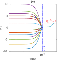
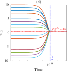
Figure 4: (a) The initial configuration. (b) The trajectories of all agents. (c) The graph of $v_{i,1}$. (d) The graph of $v_{i,2}$.

Similar to the result of Proposition 4.12, we now control the direction of the agents by adjusting the minimum value $v_{m,2}(0)$ of the initial velocity configuration for the second dimension (that is $k=2$). We first take $v_{i,2}(0)=\min\left\{v_{i,2},0.5\right\}$ for all $i\in\mathcal{I}$ as in Figure 5 (b). Figure 5 (a) is a redrawing of the velocities of the agents indicated by the arrows in Figure 4 (a). As shown in Figure 6, we can see $\lim_{t\to\infty}v_{i,2}(t)=-\left(\frac{a_{1}}{b_{1}}\right)^{\frac{1}{r-q}}=-0.5$.

Figure 5: (a) The initial velocities of agents in Figure 4. (b) The initial velocities to control the direction of the agents

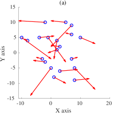
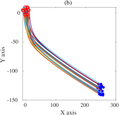
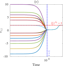
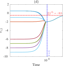
Figure 6: (a) The new initial distribution. (b) The trajectories of all agents. (c) The graph of $v_{i,1}$. (d) The graph of $v_{i,2}$.

7 Conclusion

In this study, we dicussed three open questions of the Cucker–Smale model with norm-type Rayleigh friction that were addressed in [15]. For these open questions, we proposed a more generalized model, the nonlinear Cucker–Smale model with norm-type Rayleigh friction, using the discrete $p$-Laplacian ($1<p<2$). For this model, we presented some conditions to guarantee that the norm $\left\|v_{i}\right\|_{2}$ converges to 0 or $\left(\frac{a}{b}\right)^{\frac{1}{r-q}}$ as $t\to\infty$. Moreover, we also presented conditions under which the norm $\left\|v_{i}\right\|_{2}$ converges to only $\left(\frac{a}{b}\right)^{\frac{1}{r-q}}$ as $t\to\infty$. We also proposed the nonlinear Cucker–Smale model with vector-type Rayleigh friction to discuss the open question about the direction of the velocities of agents and presented conditions to control the direction of the agents’ velocities by parameters in the model. Finally, we also showed that the regular communication weight $\psi_{R}$ satisfies the conditions given in this paper. In particular, we presented in this paper conditions that the parameter $a$ and $|v_{m,k}(0)|$ must be very small. However, we leave the question of how small they should be as a topic for future research.