The Two Quasi-Static Limits of Aether Scalar Tensor Theory

Abstract

One of the aims of Aether Scalar Tensor Theory (AeST) is to reproduce the successes of Modified Newtonian Dynamics (MOND) on galactic scales. Indeed, the quasi-static limit of AeST can achieve precisely this, assuming that the vector field $\vec{A}$ vanishes. However, this assumption of a vanishing vector field is not always justified. Here, we show how to correctly take into account the vector field and find that the quasi-static limit depends on a model parameter $m_{\times}$. In the limit $m_{\times}\to 0$, one recovers the quasi-static limit with a vanishing vector field. In particular, one finds a two-field version of MOND. In the opposite limit, $m_{\times}\to\infty$, one finds a single-field version of MOND. We show that, in practice, much of the phenomenology of the quasi-static limit depends only very little on the value of $m_{\times}$. Still, for some observational tests, such as those involving wide binaries, $m_{\times}$ has percent-level effects that may be important.

1 Introduction

Aether Scalar Tensor Theory [34, 33, AeST,] is a fully/relativistic model that reproduces much of the successes of both Modified Newtonian Dynamics [22, 21, 23, MOND,] on galactic scales and of $\Lambda$CDM on cosmological scales. It also satisfies observational constraints from gravitational waves that require tensor modes to propagate at the speed of light [32, 6].

One success of MOND that AeST aims to reproduce is explaining the observed Radial Acceleration Relation [18, 8, RAR,]. The RAR shows a one-to-one correspondence between the Newtonian acceleration due to baryons, $a_{b}$, and the actually observed acceleration, $a_{\mathrm{obs}}$. In particular, for accelerations $a_{b}$ much larger than the acceleration scale $a_{0}\approx 10^{-10}\,\mathrm{m/s}^{2}$, the total acceleration $a_{\mathrm{obs}}$ is just the Newtonian baryonic acceleration $a_{b}$. At small accelerations, $a_{b}\ll a_{0}$, the total acceleration $a_{\mathrm{obs}}$ is instead given by $a_{\mathrm{obs}}\approx\sqrt{a_{0}\,a_{b}}$.

That AeST can indeed reproduce MOND phenomenology was shown by [34] under the assumption that the vector field $\vec{A}$ (see below) vanishes. Their argument establishes that AeST reduces to a specific two-field version of MOND as long as the mass of the so-called ghost condensate is negligible [34, 29].

Here, we focus on the assumption of a vanishing vector field $\vec{A}$. In general, setting $\vec{A}$ to zero is inconsistent [29]. [34] nevertheless do so because one may expect it to be a good approximation in many situations of practical interest. Indeed, neglecting $\vec{A}$ amounts to neglecting a curl term and, in the context of MOND, neglecting curl terms was often found to be a good approximation (see, for example, [5]).

In some cases, however, curl terms can be phenomenologically important. In addition, as we will see, neglecting the vector field in AeST means neglecting a term whose prefactor can be arbitrarily large, depending on the choice of a model parameter. Thus, one might worry that the vector field cannot be neglected in cases where this prefactor is large. Here, we demonstrate that, even in these cases, AeST still reproduces MOND. More generally, we show how to correctly take the vector field $\vec{A}$ into account and discuss phenomenological implications.

In particular, we will find that the quasi-static limit of AeST depends on an additional mass parameter we call $m_{\times}$. This mass parameter $m_{\times}$ should be distinguished from another mass parameter we refer to as $m$ that controls the ghost condensate density and was studied in detail in [34, 29, 36]. In contrast to $m$, the new mass parameter $m_{\times}$ is not related to the ghost condensate and has no effect in spherical symmetry.

In the following, we employ units with $c=\hbar=1$.

2 The model

In the quasi-static weak-field limit and with only non-relativistic matter sources, the action of the AeST model reads [34, 29],

$$S=-\int d^{4}x\left\{\frac{1}{8\pi\hat{G}}\left[(\vec{\nabla}\Phi)^{2}-2\vec{\nabla}\Phi\,(\vec{\nabla}\varphi+Q_{0}\vec{A})+(\vec{\nabla}\varphi+Q_{0}\vec{A})^{2}\right.\right.\\ \left.\left.-m^{2}\left(\frac{\dot{\varphi}}{Q_{0}}-\Phi\right)^{2}+\mathcal{J}\left((\vec{\nabla}\varphi+Q_{0}\vec{A})^{2}\right)+\frac{2K_{B}}{2-K_{B}}\vec{\nabla}_{[i}\vec{A}_{j]}\vec{\nabla}^{[i}\vec{A}^{j]}\right]+\Phi\rho_{b}\right\}\,,$$ (1)

where $\Phi$ is the Newtonian gravitational potential, $\varphi$ is a scalar field, $\vec{A}$ is a vector field, and $\rho_{b}$ denotes the matter density. We use the notation $\rho_{b}$ because only the baryonic matter is relevant in the cases we discuss explicitly below. The function $\mathcal{J}$ determines how the model interpolates between the Newtonian regime (for accelerations larger than $a_{0}$) and the MOND regime (for accelerations smaller than $a_{0}$). That is, $\mathcal{J}$ determines what is called the interpolation function in MOND [10]. Further, $\hat{G}$, $Q_{0}$, $m$, and $K_{B}$ are constants with mass dimension $-2$, $1$, $1$, and $0$, respectively. In the following, we sometimes use the notation

$$\vec{U}\equiv\vec{\nabla}\varphi+Q_{0}\vec{A}\,.$$ (2)

We do not set $\dot{\varphi}$ to zero because any $\dot{\varphi}=\mathrm{const}$ also allows for static solutions. Indeed, the AeST model contains a so-called ghost condensate and $\dot{\varphi}$ represents the chemical potential of this condensate. This is explained in more detail in [29]. The term multiplied by $m^{2}$ is related to the condensate’s energy density.

The constant $\hat{G}$ is related to the Newtonian gravitational constant $G_{N}$ as

$$G_{N}\equiv\hat{G}\,f_{G}^{-1}\,,$$ (3)

with constant $f_{G}$. Here, $G_{N}$ is what enters the total acceleration felt by matter in the Newtonian regime, i.e. at accelerations larger than $a_{0}$. That is, in spherical symmetry and in the Newtonian regime, the total acceleration has the form $G_{N}M/r^{2}$ with the total mass $M$ and the spherical radius $r$.

The function $\mathcal{J}$ must satisfy some requirements that ensure that there is a Newtonian regime at large accelerations and a MOND regime at small accelerations. In particular, the interpolation function $\tilde{\mu}(|\vec{U}|/a_{0})\equiv\mathcal{J}^{\prime}(\vec{U}^{2})$ must have the limits [34, 10],

$$\left.\tilde{\mu}\left(\frac{|\vec{U}|}{a_{0}}\right)\right|_{\frac{|\vec{U}|}{a_{0}}\to 0}=f_{G}\,\frac{|\vec{U}|}{a_{0}}\,,\quad\left.\tilde{\mu}\left(\frac{|\vec{U}|}{a_{0}}\right)\right|_{\frac{|\vec{U}|}{a_{0}}\to\infty}=\frac{f_{G}}{1-f_{G}}\,.$$ (4)

In the following, we adopt $a_{0}=1.2\cdot 10^{-10}\,\mathrm{m/s}^{2}$ [18].

In AeST, ordinary matter is minimally coupled to the metric $g_{\mu\nu}$ in the standard way. The metric has the same form as in the Newtonian limit of General Relativity with the potential $\Phi$. There is no additional coupling of matter to the fields $\varphi$ and $\vec{U}$. Thus, the total acceleration felt by matter is

$$\vec{a}_{\mathrm{tot}}\equiv-\vec{\nabla}\Phi\,.$$ (5)

Like matter, light is also minimally coupled to the metric $g_{\mu\nu}$ in the standard way (although this is not shown explicitly in Eq. (1)). Thus, lensing works as in General Relativity, just with the potential $\Phi$ calculated from different field equations [33, 29].

3 Why one may be cautious about leaving out the vector field

To set the stage, we first assume a vanishing vector field $\vec{A}$ and show that this assumption is, in general, inconsistent. Nevertheless, as mentioned above, one may expect that neglecting $\vec{A}$ is a good approximation in many situations of practical interest. Here, we discuss why this is the case and why, in some cases, one may still be cautious about neglecting $\vec{A}$.

With $\vec{A}$ set to zero, the equations of motion for the remaining fields $\varphi$ and $\Phi$ read [34],

$$\Delta\hat{\Phi} =f_{G}\cdot 4\pi G_{N}\left(\rho_{b}+\rho_{c}\right)\,,$$ (6a)

$$\vec{\nabla}\left(\tilde{\mu}\left(\frac{|\vec{\nabla}\varphi|}{a_{0}}\right)\vec{\nabla}\varphi\right) =f_{G}\cdot 4\pi G_{N}\left(\rho_{b}+\rho_{c}\right)\,,$$ (6b)

where we defined

$$\hat{\Phi}=\Phi-\varphi\,,$$ (7)

and where $\rho_{c}$ is the density of the ghost condensate,

$$\rho_{c}=\frac{m^{2}}{4\pi G_{N}f_{G}}\left(\frac{\dot{\varphi}}{Q_{0}}-\hat{\Phi}-\varphi\right)\,.$$ (8)

The total acceleration $\vec{a}_{\mathrm{tot}}=-\vec{\nabla}\Phi$ can be written as the sum of the accelerations $\vec{a}_{\varphi}=-\vec{\nabla}\varphi$ and $\vec{a}_{\hat{\Phi}}=-\vec{\nabla}\hat{\Phi}$ due to the fields $\varphi$ and $\hat{\Phi}$, respectively,

$$\vec{a}_{\mathrm{tot}}=\vec{a}_{\varphi}+\vec{a}_{\hat{\Phi}}\,.$$ (9)

These equations give MOND-like behavior whenever the effects of the condensate density $\rho_{c}$ are negligible. To see this, consider a spherically symmetric system and consider first the large-acceleration regime $a_{b}\gg a_{0}$. Then, using the limits of $\tilde{\mu}$ from Eq. (4), we find

$$a_{\varphi}=(1-f_{G})a_{b}\,,\quad a_{\hat{\Phi}}=f_{G}\,a_{b}\,,$$ (10)

which gives

$$a_{\mathrm{tot}}=a_{b}\,,$$ (11)

which is exactly what MOND requires in this large-acceleration regime. Similarly, in the small-acceleration regime, $a_{b}\ll a_{0}$, we find

$$a_{\mathrm{tot}}\approx a_{\varphi}\approx\sqrt{a_{0}a_{b}}\,,$$ (12)

which again matches MOND. Thus, AeST seems to have achieved its goal of reproducing MOND-like behavior. In particular, AeST seems to reproduce a multifield version of MOND [10].

The problem is that setting $\vec{A}$ to zero is not always allowed. To see this, consider the $\vec{A}$ equation of motion,

$$\vec{\nabla}\Phi-\frac{1}{2Q_{0}}\frac{2K_{B}}{2-K_{B}}\vec{\nabla}\times\vec{\nabla}\times\vec{A}=(\vec{\nabla}\varphi+Q_{0}\vec{A})\left(1+\mathcal{J}^{\prime}\left((\vec{\nabla}\varphi+Q_{0}\vec{A})^{2}\right)\right)\,.$$ (13)

If it is allowed to set $\vec{A}$ to zero, this equation must be satisfied with $\vec{A}=0$,

$$\vec{\nabla}\Phi=(\vec{\nabla}\varphi)\left(1+\mathcal{J}^{\prime}\left((\vec{\nabla}\varphi)^{2}\right)\right)\,.$$ (14)

We can algebraically solve this equation for $\vec{\nabla}\varphi$ and then take the curl to find

$$\vec{\nabla}|\vec{\nabla}\Phi|\times\vec{\nabla}\Phi=0\,.$$ (15)

This condition is not fulfilled, except in some special cases like spherical symmetry [7]. This is important because for many systems of astrophysical interest – such as disk galaxies – one cannot assume spherical symmetry or another of the special cases where Eq. (15) holds.

Thus, in general, setting $\vec{A}$ to zero is inconsistent. Even so, neglecting $\vec{A}$ may still be a good approximation. Indeed, consider a Helmholtz decomposition of $\vec{A}$,

$$\vec{A}=\vec{\nabla}\alpha_{A}+\vec{\nabla}\times\vec{\beta}_{A}\,.$$ (16)

[33] show that $\alpha_{A}$ can be absorbed into $\varphi$, so that neglecting $\vec{A}$ amounts to neglecting only the curl term $\vec{\nabla}\times\vec{\beta}_{A}$. In the context of MOND, neglecting curl terms is often a good approximation (see, for example, [5]). So one might expect a similar result here.

However, there is also reason to be cautious. In AeST, neglecting the vector field $\vec{A}$ implies neglecting the following term in Eq. (13),

$$-\frac{1}{2Q_{0}}\frac{2K_{B}}{2-K_{B}}\vec{\nabla}\times\vec{\nabla}\times\vec{A}\,.$$ (17)

The prefactor of this term can be arbitrarily large, depending on the choice of the model parameters $Q_{0}$ and $K_{B}$. Thus, at least when this prefactor is large, one may worry that neglecting $\vec{A}$ is a bad approximation. Below, we discuss what happens in this case and, more generally, show how to correctly take the vector field into account.

4 Taking the vector field into account

We now show how to correctly take the vector field $\vec{A}$ into account and establish that AeST still reproduces MOND-like behavior, though not always in the way the $\vec{A}=0$ case suggests. We discuss the phenomenological implications in Sec. 6 and Sec. 7.

We first write the action in terms of $\vec{U}$,

$$S=-\int d^{4}x\left\{\frac{1}{8\pi\hat{G}}\left[(\vec{\nabla}\Phi)^{2}-2\vec{\nabla}\Phi\,\vec{U}+\vec{U}^{2}\right.\right.\\ \left.\left.-m^{2}\left(\frac{\dot{\varphi}}{Q_{0}}-\Phi\right)^{2}+\mathcal{J}\left(\vec{U}^{2}\right)+\frac{1}{m_{\times}^{2}}\vec{\nabla}_{[i}\vec{U}_{j]}\vec{\nabla}^{[i}\vec{U}^{j]}\right]+\Phi\rho_{b}\right\}\,,$$ (18)

where we used $Q_{0}^{2}\,\vec{\nabla}_{[i}\vec{A}_{j]}=\vec{\nabla}_{[i}\vec{U}_{j]}$ which follows from antisymmetry, and we defined the mass scale

$$m_{\times}\equiv\sqrt{\frac{2-K_{B}}{2K_{B}}}Q_{0}\,.$$ (19)

The equation of motion of $\varphi$ is then of the form $\partial_{t}(\dot{\varphi}-Q_{0}\Phi)=0$ which is trivially satisfied in the quasi-static limit (keeping in mind that the only time-dependence we allow is $\dot{\varphi}=\mathrm{const}$). This leaves the equations of motion of $\Phi$ and $\vec{U}$. They read

$$\Delta\Phi-\vec{\nabla}\vec{U} =4\pi G_{N}f_{G}(\rho_{b}+\rho_{c})\,,$$ (20a)

$$\vec{\nabla}\Phi-\frac{1}{m_{\times}^{2}}\vec{\nabla}\times\vec{\nabla}\times\vec{U} =\vec{U}\left(1+\tilde{\mu}\left(\frac{|\vec{U}|}{a_{0}}\right)\right)\,.$$ (20b)

These are the equations that must be solved in the quasi-static limit of AeST. They replace Eq. (6) when one correctly takes the vector field into account. In spherical symmetry, they are equivalent to the equations Eq. (6), see Sec. 6, but in general they are not.

To see that the equations Eq. (20) still describe MOND-like behavior, we will first discuss the limits of large and small $m_{\times}$. We will find that both describe a version of MOND. In particular, for $m_{\times}\to 0$, one recovers the two-field version of MOND from Eq. (6). That is, setting $\vec{A}$ to zero is justified in this case (but not in general). In the opposite limit, $m_{\times}\to\infty$, one recovers a single-field version of MOND. Plausibly, other values of $m_{\times}$ interpolate between these single-field and two-field versions of MOND.

4.1 The limit $m_{\times}\to\infty$: A single-field version of MOND

The complicated part of the equations of motion Eq. (20) is the double-curl term proportional to $1/m_{\times}^{2}$ in the $\vec{U}$ equation of motion. Luckily, for $m_{\times}\to\infty$, this term vanishes and we can algebraically solve for $\vec{U}$. We choose to write the result in the following form,

$$\vec{U}=\vec{\nabla}\Phi\left(1-f_{G}\,\mu\left(\frac{|\vec{\nabla}\Phi|}{a_{0}}\right)\right)\,,$$ (21)

which implicitly defines the function $\mu$ in terms of the function $\tilde{\mu}$. From the limiting behavior of $\tilde{\mu}$, Eq. (4), we can infer the limiting behavior of $\mu$, namely

$$\left.\mu\left(\frac{|\vec{\nabla}\Phi|}{a_{0}}\right)\right|_{\frac{|\vec{\nabla}\Phi|}{a_{0}}\to 0}=\frac{|\vec{\nabla}\Phi|}{a_{0}}\,,\quad\left.\mu\left(\frac{|\vec{\nabla}\Phi|}{a_{0}}\right)\right|_{\frac{|\vec{\nabla}\Phi|}{a_{0}}\to\infty}=1\,.$$ (22)

This is the correct behavior for a single-field MOND interpolation function [10].

Indeed, plugging this solution for $\vec{U}$ into the $\Phi$ equation of motion Eq. (20a) gives

$$\vec{\nabla}\left(\mu\left(\frac{|\vec{\nabla}\Phi|}{a_{0}}\right)\vec{\nabla}\Phi\right)=4\pi G_{N}(\rho_{b}+\rho_{c})\,,$$ (23)

which is a standard single-field version of MOND [5, 10] up to the ghost condensate density $\rho_{c}$. Without the ghost condensate, this is known as aquadratic Lagrangian theory (AQUAL).

This shows that the $m_{\times}\to\infty$ limit of AeST reproduces MOND-like behavior as long as the effects of the ghost condensate density are negligible. In particular, AeST reproduces a single-field version of MOND in this limit.

4.2 The limit $m_{\times}\to 0$: A two-field version of MOND

In the opposite limit, $m_{\times}\to 0$, we cannot neglect the double-curl term multiplied by $1/m_{\times}^{2}$. To deal with this term, we use the Helmholtz decomposition. One particular implication of this decomposition is that, instead of solving a vector field equation $\vec{X}=0$ one can equivalently solve the system of equations $\vec{\nabla}\cdot\vec{X}=0$ and $\vec{\nabla}\times\vec{X}=0$ with the boundary condition that $\vec{X}$ vanishes at infinity [13].

We apply this to the $\vec{U}$ equation of motion Eq. (20b). This gives the two equations

$$\Delta\Phi=\vec{\nabla} \left[\vec{U}\left(1+\tilde{\mu}\left(\frac{|\vec{U}|}{a_{0}}\right)\right)\right]\,,$$ (24a)

$$-\vec{\nabla}\times\vec{\nabla}\times\vec{\nabla}\times\vec{U}=m_{\times}^{2}\,\vec{\nabla}\times \left[\vec{U}\left(1+\tilde{\mu}\left(\frac{|\vec{U}|}{a_{0}}\right)\right)\right]\,,$$ (24b)

with the reasonable boundary conditions that $\vec{U}$ and $\vec{\nabla}\Phi$ vanish at infinity. We also decompose the field $\vec{U}$ itself into a divergence-less and a curl-less part,

$$\vec{U}=\vec{U}_{\times}+\vec{\nabla}\alpha\,,$$ (25)

where $\vec{U}_{\times}$ is a vector field with $\vec{\nabla}\cdot\vec{U}_{\times}=0$ and $\alpha$ is a scalar field. This Helmholtz decomposition is guaranteed to exist when $\vec{U}$ vanishes at least as fast as $1/r$ for $r\to\infty$. We assume that to be true for now. Below we will see that this is justified for physically reasonable solutions.

We now consider the implications of the limit $m_{\times}\to 0$. The only equation where $m_{\times}$ appears is the curl-part of the $\vec{U}$ equation Eq. (24b). Using the Helmholtz decomposition of $\vec{U}$ Eq. (25), we find

$$\vec{\nabla}\times\vec{\nabla}\times\vec{\nabla}\times\vec{U}_{\times}=\mathcal{O}(m_{\times}^{2})\,.$$ (26)

Let’s assume that $\vec{U}_{\times}$ (and not just $\vec{U}$ itself) vanishes at infinity. Then, we find

$$\vec{U}_{\times}=\mathcal{O}(m_{\times}^{2})\,,$$ (27)

by repeatedly applying the theorem mentioned at the very beginning of this section. Thus, in the limit $m_{\times}\to 0$, the vector field $\vec{U}$ is just the gradient of a scalar field,

$$\vec{U}=\vec{\nabla}\alpha+\mathcal{O}(m_{\times}^{2})\,.$$ (28)

We can plug this result back into the remaining two equations, namely the divergence-part of the $\vec{U}$ equation of motion Eq. (24a) and the $\Phi$ equation of motion Eq. (20a),

$$\Delta(\Phi-\alpha) =4\pi G_{N}f_{G}(\rho_{b}+\rho_{c})\,,$$ (29)

$$\vec{\nabla}\left(\tilde{\mu}\left(\frac{|\vec{\nabla}\alpha|}{a_{0}}\right)\vec{\nabla}\alpha\right) =\Delta(\Phi-\alpha)\,.$$ (30)

This can be rewritten as

$$\Delta(\Phi-\alpha) =4\pi G_{N}f_{G}(\rho_{b}+\rho_{c})\,,$$ (31)

$$\vec{\nabla}\left(\tilde{\mu}\left(\frac{|\vec{\nabla}\alpha|}{a_{0}}\right)\vec{\nabla}\alpha\right) =4\pi G_{N}f_{G}(\rho_{b}+\rho_{c})\,.$$ (32)

This is equivalent to the system of equations Eq. (6) obtained by setting the vector field $\vec{A}$ to zero, just with $\vec{\nabla}\varphi$ replaced by $\vec{\nabla}\alpha$. Thus, the procedure of [34] is justified in the $m_{\times}\to 0$ limit.

For the original equations of motion obtained by [34], Eq. (6), the field $\vec{\nabla}\varphi$ does fall off at least as fast as $1/r$ for physical solutions [34, 29]. Thus, at least in the limit $m_{\times}\to 0$, the same is true for $\vec{\nabla}\alpha=\vec{U}$ and the decomposition of $\vec{U}$ given in Eq. (25) does indeed exist.

This shows that the $m_{\times}\to 0$ limit of AeST reproduces MOND-like behavior as long as the effects of the ghost condensate density are negligible. In particular, AeST reproduces a two-field version of MOND in this limit.

5 Scale-dependence of the two limits

Above, we have seen that AeST reduces to a single-field version of MOND for $m_{\times}\to\infty$ and to a two-field version for $m_{\times}\to 0$. In practice, whether the single-field or the two-field limit is applicable depends not only on the value of the model parameter $m_{\times}$. It also depends on the system under consideration. In particular, consider a system with typical length scale $l$. Then, derivatives can very roughly be estimated to be of order $1/l$. Thus, in practice, the relevant quantity is $m_{\times}l$ (see Eq. (20b)),

$$m_{\times}l\gg 1 :\quad\mathrm{single-field\;limit}\,,$$ (33)

$$m_{\times}l\ll 1 :\quad\mathrm{two-field\;limit}\,.$$ (34)

That is, even after fixing the AeST model parameters, some systems will behave as in a single-field version of MOND while others will behave as in a two-field version of MOND.

The quantity $m_{\times}=\sqrt{(2-K_{B})/K_{B}}Q_{0}$ is, to the best of our knowledge, not yet constrained phenomenologically. For the explicit examples of model parameters given in [34], we have

$$10^{-4}\,\mathrm{Mpc}^{-1}\lesssim m_{\times}\lesssim 1\,\mathrm{Mpc}^{-1}\,.$$ (35)

Thus, in the following, we will assume this range of parameter values, though other choices are certainly possible. For this range of parameter values, the transition from the two-field limit (small spatial scales) to the single-field limit (large spatial scales) happens for $l\sim\mathrm{Mpc}$ or larger.

To be concrete, this means that the two-field limit is relevant for wide binaries ($l\sim\mathrm{kAU}$), and at least the inner parts of galaxies ($l\sim\mathrm{kpc}$). For galaxy clusters ($l\sim\mathrm{Mpc}$), the single-field limit may be relevant depending on the details of the cluster under consideration and the precise value of $m_{\times}$.

6 Galactic rotation curves are almost the same in both limits

Above, we have seen that the quasi-static limit of AeST is more complicated than what [34] have proposed based on the assumption of a vanishing vector field $\vec{A}$. The procedure of [34] is justified for systems much smaller than the model parameter $1/m_{\times}$, but not in general. In practice, however, the value of $m_{\times}$ is often unimportant. That is, in practice, one can often follow the procedure of [34] even for systems larger than $1/m_{\times}$.

One particular example is spherical symmetry. In this case, the value of $1/m_{\times}$ is irrelevant. That’s simply a consequence of the fact that $1/m_{\times}^{2}$ enters only as the prefactor of a curl term which must vanish in spherical symmetry. In that case, one finds the algebraic MOND-like relation,

$$a_{\mathrm{tot}}=a_{N}\,\nu\left(\frac{|a_{N}|}{a_{0}}\right)\,,$$ (36)

independently of the value of $m_{\times}$. Here, $a_{N}$ is the Newtonian acceleration due to the mass corresponding to the density $\rho\equiv\rho_{b}+\rho_{c}$, which includes both the baryonic matter and the ghost condensate. The function $\nu$ can be found from $\mu$ by solving $\mu(x)x=y$ for $x$ and writing the result in the form $\nu(y)y=x$ [10]. Thus, in the case where the ghost condensate is negligible, this gives the standard MOND relation $a_{\mathrm{tot}}=a_{b}\,\nu(a_{b}/a_{0})$.

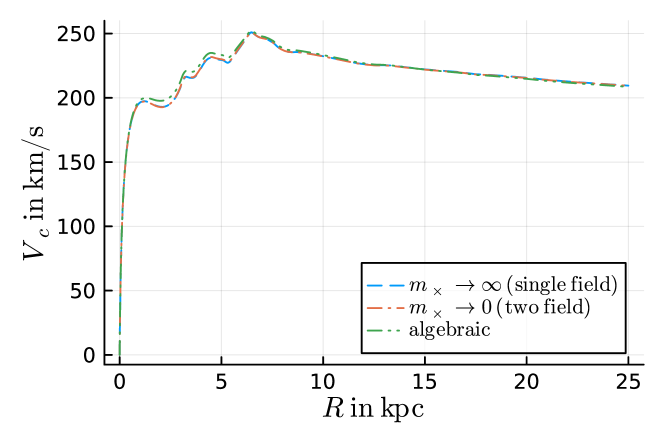
Figure 1: The rotation curve of the Milky Way for the single-field limit $m_{\times}\to 0$ (dashed blue line), the two-field limit $m_{\times}\to 0$ (dash-dotted red line), and as calculated from the algebraic MOND relation Eq. (36). This is with the simple interpolation function $\mu(x)=x/(1+x)$, $f_{G}=0.99$, and without the ghost condensate mass, i.e. for $m^{2}/f_{G}=0$. We assume the Milky Way mass model from [20].

Many astrophysically relevant systems are not spherically symmetric, of course. But even in axisymmetric systems does the value of $m_{\times}$ not matter in practice. This can be seen from Fig. 1, which shows the Milky Way rotation curve as calculated for the two limits $m_{\times}\to 0$ and $m_{\times}\to\infty$ for the Milky Way mass model from [20]. Here, we assume $m^{2}/f_{G}=0$ for simplicity. That is, we assume that the ghost condensate density vanishes. This is a good approximation at the radii considered here, at least for the usual choice $\sqrt{f_{G}}/m\gtrsim\mathrm{Mpc}$ [34, 29]. Details of the numerical procedure are described in Appendix A.

For reference, Fig. 1 also shows a rotation curve obtained from the algebraic relation Eq. (36). This algebraic relation is often considered a reasonable approximation in MOND. We see that the difference between the $m_{\times}\to 0$ and $m_{\times}\to\infty$ limits is much smaller than that between the algebraic case and either value of $m_{\times}$. Indeed, the effect of $m_{\times}$ is much smaller than the systematic uncertainties in modelling the Milky Way [20]. Thus, in practice, the value of $m_{\times}$ is unlikely to play a role for galactic rotation curves.

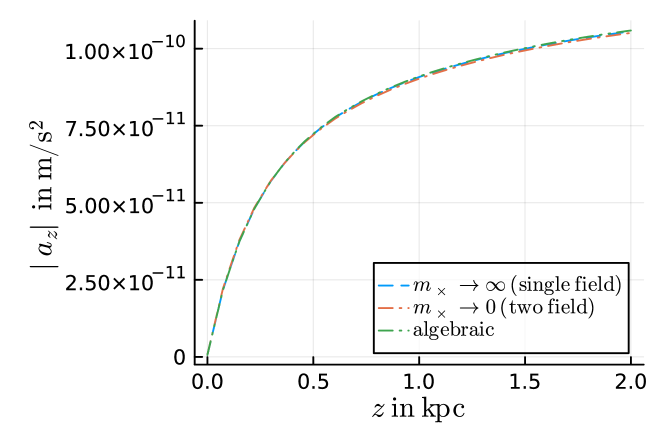
Figure 2: The vertical acceleration for the same Milky Way model as shown in Fig. 1 at the solar radius $R=8.1\,\mathrm{kpc}$ for the single-field limit $m_{\times}\to\infty$ (dashed blue line), the two-field limit $m_{\times}\to 0$ (dash-dotted red line), and as calculated from the algebraic MOND relation from Eq. (36).

The same holds for observables based on the vertical acceleration above the Milky Way disk (see for example [19, 37]). This is illustrated in Fig. 2 which shows almost no difference between the limits $m_{\times}\to 0$ and $m_{\times}\to\infty$.

7 Percent-level effect for wide binaries

Since the field equations of MOND are inherently non-linear, the environment of a system can affect its internal dynamics. This is the so-called External Field Effect (EFE) and it violates the Strong Equivalence Principle. For us, the important thing is that single-field and two-field versions of MOND do not produce the same EFE [26].

One particular type of system where the EFE is important are wide binaries [16, 4, 3, 30, 15, see, for example, ]. Intriguingly, recent observational studies of wide binaries are getting close to percent-level accuracy in acceleration [31, 14, 9]. Thus, even small differences in what AeST predicts compared to other models can be important.

As discussed in Sec. 5, the two-field limit $m_{\times}\to 0$ of AeST is the relevant one for wide binaries. Previous works have not considered this two-field version of MOND, focusing on other models such as that obtained in the $m_{\times}\to\infty$ limit of AeST [4, 3, i.e. AQUAL,]. Thus, any difference between these two limits indicates that the AeST prediction for wide binaries deviates from what previous studies considered. In this regard, a more general point is that different models that reproduce the same basic tenets of MOND, such as being able to explain the RAR, may differ in their secondary predictions such as the size of the EFE [27, 24].

As we will now show, there can indeed be percent-level differences between the single-field and and two-field limits of AeST. However, there’s also reason to be careful with quantitative statements. As we will argue, in the two-field limit, wide binaries are much more sensitive to the details of the local Galactic field than in the single-field limit. Any quantitative statement about the difference between these two limits must be understood to be relative to a particular model of the Milky Way and it is plausible that different Milky Way models erase or significantly enhance the percent-level differences mentioned above.

To see this, we again assume that the ghost condensate’s mass is not important or, equivalently, that $m^{2}/f_{G}=0$. This is a good approximation on the small scales, $l\sim\mathrm{kAU}$, that are relevant here. We also assume that the EFE dominates everywhere in the wide binary system under consideration. This approximation is reasonable when the distance between the two stars in the binary system is relatively large [4, 3]. Importantly, these approximations allow us to make analytical estimates. More involved numerical calculations are left for future work.

As already mentioned, for the internal dynamics wide binaries, the two-field limit $m_{\times}\to 0$ is the relevant one. For simplicity, we assume that the external field produced by the Milky Way can be calculated using the same limit. We expect this to be a good approximation, since the $m_{\times}\to 0$ limit is valid up to scales of order $1/m_{\times}$ which in our case means up to $1\,\mathrm{Mpc}-10^{4}\,\mathrm{Mpc}$. Thus, we generally expect only sub-percent differences between the actual external field and that calculated using the $m_{\times}\to 0$ limit.

For reference, we first consider the single-field limit $m_{\times}\to\infty$, assuming that the external field is also calculated in this limit. This is equivalent to AQUAL and is explicitly discussed in [4]. They find for the radial acceleration in the binary system, $a$, relative to that in the Newtonian case, $a_{N}$,

$$\left.\frac{a}{a_{N}}\right|_{m_{\times}\to\infty}=\frac{1}{\mu(x_{e})\sqrt{1+\sin^{2}\theta\,L(x_{e})}}\,.$$ (37)

Here, $\mu(x)$ is the interpolation function of single-field MOND (see Sec. 4.1), $L(x)$ is its logarithmic derivative,

$$L(x)\equiv\frac{x\mu^{\prime}(x)}{\mu(x)}\,,$$ (38)

$x_{e}$ is the gradient of the external gravitational potential $\Phi_{e}$ relative to $a_{0}$,

$$x_{e}=\frac{|\vec{\nabla}\Phi_{e}|}{a_{0}}\,,$$ (39)

and $\theta$ is the angle between the radial direction (connecting the two stars in the binary system) and the external field.

It is straightforward to adopt the procedure of [4] to the two-field limit $m_{\times}\to 0$. We find

$$\left.\frac{a}{a_{N}}\right|_{m_{\times}\to 0}=f_{G}\left(1+\frac{1}{\tilde{\mu}(x_{\varphi,e})\sqrt{1+\sin^{2}\theta\,\tilde{L}(x_{\varphi,e})}}\right)\,,$$ (40)

where $\tilde{\mu}(x)$ is the two-field version of the interpolation function (see Sec. 4.2), $\tilde{L}(x)$ is its logarithmic derivative, and $x_{\varphi,e}$ is the gradient of the external gravitational potential $\varphi_{e}$ relative to $a_{0}$,

$$x_{\varphi,e}=\frac{|\vec{\nabla}\varphi_{e}|}{a_{0}}\,.$$ (41)

This expression for $a/a_{N}$ has a very similar structure as the corresponding single-field expression Eq. (37), except there are now two terms, corresponding to the two fields $\Phi$ and $\varphi$, the single-field interpolation function $\mu$ is replaced with its two-field counterpart $\tilde{\mu}$, and there is an overall factor of $f_{G}$.

Importantly, in the two-field limit, it is only the external field of the field $\varphi$ that plays a role, the external field of $\Phi$ is irrelevant. This is because the $\Phi$ equation of motion is linear so that there is no EFE.

This is related to an important complication in the two-field limit, regarding how to choose the value of $x_{\varphi,e}$. In the single-field limit, a simple way to choose the external gravitational field is to reproduce the observed circular rotation curve of the Milky Way at the solar radius,

$$x_{e}=\frac{|\vec{\nabla}\Phi_{e}|}{a_{0}}\equiv\frac{1}{a_{0}}\frac{V_{c}^{2}}{R_{\odot}}\,.$$ (42)

In the two-field limit, reproducing the value of $V_{c}^{2}/R_{\odot}$ means

$$x_{\Phi,e}+x_{\varphi,e}=|\vec{\nabla}\Phi_{e}+\vec{\nabla}\varphi_{e}|\equiv\frac{1}{a_{0}}\frac{V_{c}^{2}}{R_{\odot}}\,,$$ (43)

where $x_{\Phi,e}\equiv|\vec{\nabla}\Phi_{e}|/a_{0}$ and, for simplicity, we assumed that $\vec{\nabla}\Phi_{e}$ and $\vec{\nabla}\varphi_{e}$ point in the same direction. The important point is that, in the single-field case, the observed value of $V_{c}^{2}/R_{\odot}$ directly gives $x_{e}$ and that is all that is needed to calculate $a/a_{N}$ from Eq. (37). This is different in the two-field case. The observed value of $V_{c}^{2}/R_{\odot}$ only gives the sum $x_{\Phi,e}+x_{\varphi,e}$ while calculating $a/a_{N}$ from Eq. (40) requires the $x_{\varphi,e}$ part of that sum individually.

This is the complication for the two-field case mentioned above. It requires additional assumptions about the external field to know which part of the total acceleration $V_{c}^{2}/R_{\odot}$ comes from $\Phi$ and which part comes from $\varphi$.

Here, we first consider a spherically symmetric external field. Of course, the Milky Way is not spherically symmetric, but this case serves as an illustrative starting point. We discuss more general cases below. Assuming spherical symmetry, the total acceleration $x_{\mathrm{tot},e}\equiv|\vec{\nabla}\Phi_{e}+\vec{\nabla}\varphi_{e}|/a_{0}$ in the two-field case satisfies the standard algebraic MOND relation with the interpolation function $\mu$ from the single-field limit,

$$\mu(x_{\mathrm{tot},e})\,x_{\mathrm{tot},e}=y_{e}\,,$$ (44)

where $y_{e}$ is the gradient of the Newtonian external potential relative to $a_{0}$. This follows from Eq. (31) in spherical symmetry and the definition of $\mu$ in terms of $\tilde{\mu}$ Eq. (21). In addition, we have $x_{\Phi,e}=f_{G}\,y_{e}$ directly from Eq. (31). This gives

$$x_{\varphi,e}=x_{\odot}(1-f_{G}\mu(x_{\odot}))\,\quad\mathrm{with}\quad x_{\odot}\equiv\frac{1}{a_{0}}\frac{V_{c}^{2}}{R_{\odot}}\,.$$ (45)

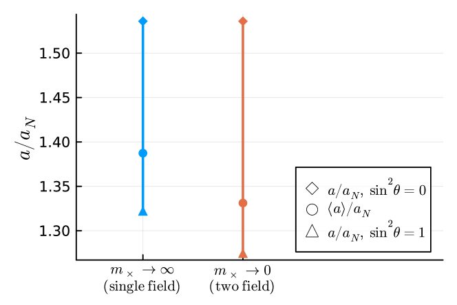
Figure 3: The radial acceleration in a wide binary system relative to that in the Newtonian case for the single-field limit $m_{\times}\to\infty$ (blue) and the two-field limit $m_{\times}\to 0$ (red) of AeST. For real-world wide binaries with separations $l\sim\mathrm{kAU}$, the two-field limit $m_{\times}\to 0$ is the relevant one. Markers with a diamond shape indicate an external field parallel to the radial direction, $\sin^{2}\theta=0$, markers with a triangle shape indicate a perpendicular external field, $\sin^{2}\theta=1$, and markers with a circle shape indicate the angular average from Eq. (47). We assume that the external field dominates everywhere in the binary system and use the simple interpolation function $\mu(x)=x/(1+x)$. We further assume $f_{G}=0.99$ and no ghost condensate mass, i.e. $m^{2}/f_{G}=0$. The external field is calculated from the acceleration $V_{c}^{2}/R$ at the solar radius $R=8.1\,\mathrm{kpc}$ for the Milky Way model shown in Fig. 1. For the single-field limit, the value of $V_{c}^{2}/R$ alone suffices to calculate $a/a_{N}$. For the two-field limit, we additionally assume the algebraic MOND relation Eq. (36).

Thus, assuming spherical symmetry, we can calculate $a/a_{N}$ from just $V_{c}^{2}/R_{\odot}$ even in the two-field limit. Explicitly,

$$\left.\frac{a}{a_{N}}\right|^{\mathrm{spherical}}_{m_{\times}\to 0}=\left.f_{G}\left(1+\frac{1}{\tilde{\mu}(x_{\varphi,e})\sqrt{1+\sin^{2}\theta\,\tilde{L}(x_{\varphi,e})}}\right)\right|_{x_{\varphi,e}=x_{\odot}(1-f_{G}\mu(x_{\odot}))}\,,$$ (46)

with $x_{\odot}$ as defined in Eq. (45). This should be compared to the single-field result Eq. (37) with $x_{e}=x_{\odot}$. We quantitatively compare these two cases in Fig. 3.

From Fig. 3, we see that the two-field and the single-field limits give the same acceleration when the external field points in the radial direction, $\sin^{2}\theta=0$. In contrast, when the external field is perpendicular, $\sin^{2}\theta=1$, the acceleration in the two-field limit is a few percent smaller than in the single-field limit. [3] also consider an acceleration averaged over $\theta$,

$$\langle a\rangle\equiv\frac{1}{2}\int_{0}^{\pi}d\theta\sin\theta\,a\,.$$ (47)

As we can see from Fig. 3, this averaged acceleration is again smaller for the two-field limit than for the single-field limit. The magnitude of the effect after averaging is similar to that in the perpendicular case without averaging.

These results are often a good approximation even beyond spherical symmetry, namely whenever the algebraic relation $\mu(x_{\mathrm{tot},e})\,x_{\mathrm{tot},e}=y_{e}$ from Eq. (44) is a good approximation. This is indeed often the case, see for example [5, 17].

However, one also must be careful here. Since the difference between the single-field and the two-field limits is just a few percent, one should use the algebraic relation Eq. (44) only if it is valid well below the percent level. Otherwise, any real effect may be washed out by errors in the external field.

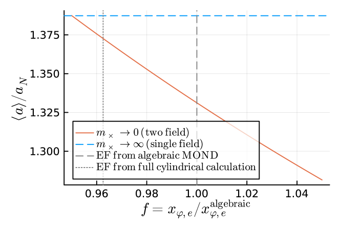
Figure 4: The angle-averaged acceleration Eq. (47) in a wide binary system relative to the Newtonian case as a function of how much the external field $x_{\varphi,e}$ in the two-field limit $m_{\times}\to 0$ deviates from what the algebraic relation Eq. (36) implies (solid red line). For comparison we also show the single-field limit $m_{\times}\to\infty$ (dashed blue line) which does not depend on $f$. Apart from this factor $f$, the calculation is the same as in Fig. 3. The vertical dashed line denotes the prediction for an external field that follows the algebraic MOND relation, $f=1$, while the dotted vertical line shows what we find for the axisymmetric Milky Way model from [20], see also Fig. 1.

We show the effect of deviations from the algebraic relation Eq. (44) in Fig. 4. In particular, we show how the averaged acceleration ratio $\langle a\rangle/a_{N}$ in the two-field limit changes when the gradient of the external field $x_{\varphi,e}$ deviates from what the algebraic relation Eq. (44) says it should be. We parametrize the deviation of $x_{\varphi,e}$ from its value derived from this algebraic relation by a factor $f$,

$$f\equiv\frac{x_{\varphi,e}}{x_{\varphi,e}^{\mathrm{algebraic}}}\equiv\frac{x_{\varphi,e}}{x_{\odot}(1-f_{G}\mu(x_{\odot}))}\,.$$ (48)

From Fig. 4, we see that a deviation of $x_{\varphi,e}$ from its algebraic value by a few percent also changes the acceleration $\langle a\rangle/a_{N}$ by a few percent. In particular, smaller values of $x_{\varphi,e}$ bring the single-field and the two-field limit closer together, while larger values push them apart. A moderately smaller value, $f\approx 0.95$, erases the difference between the two limits.

Thus, compared to the single-field limit, one needs to know the details of the Milky Way’s gravitational field much more precisely when making predictions for wide binaries in the two-field limit. As one particular example, we here consider the axisymmetric Milky Way model already discussed in Sec. 6. In that model, comparing the numerically computed value of $x_{\varphi,e}$ at the solar radius to that inferred from the algebraic relation Eq. (44) gives

$$f\approx 0.963\,.$$ (49)

This value is also highlighted in Fig. 4. We see that this leaves a difference of only about $1.5$ percentage points between the single-field and the two-field limit.

One might conclude that the value of $m_{\times}$ makes very little difference for wide binaries. That is, one might expect that the AeST prediction (corresponding to the two-field limit $m_{\times}\to 0$) is very close to what previous studies have found for AQUAL (i.e. for the single-field limit $m_{\times}\to\infty$). However, as we have seen, any quantitative statement depends sensitively on the details of the local gravitational field of the Milky Way. Indeed, the Milky Way disk is found not to be in equilibrium and non-axisymmetries may not be negligible [1, 11, 20]. Plausibly, such effects can either erase or significantly enhance the percent-level differences between AeST and other models of MOND. Thus, quantitative predictions require more involved numerical studies that take such effects into account. They also require carefully evaluating how accurate such predictions can be given the observational uncertainties. This is left for future work.

8 Conclusion

Previous discussions of the quasi-static limit of AeST have assumed that the vector field $\vec{A}$ vanishes. Here, we have shown that this assumption is, in general, not justified. We have also shown how to correctly take the vector field into account. In particular, we find that the quasi-static limit depends on a model parameter $m_{\times}$. In the limits $m_{\times}\to\infty$ and $m_{\times}\to 0$ one recovers a single-field and a two-field version of MOND, respectively. The two-field version of MOND is precisely what was found in previous works where the vector field was neglected. Thus, these previous works are justified in the limit $m_{\times}\to 0$, but not in general.

For finite values of $m_{\times}$, the quasi-static limit of AeST represents a novel version of MOND that does not reduce to any of the previously-proposed versions such as AQUAL [5], quasi-linear MOND [28, 24, QUMOND,], or modified inertia [25].

In practice, however, numerical calculations indicate that the value of $m_{\times}$ makes almost no difference for radial and vertical accelerations in galaxies. Thus, for rotation curves, for example, our results are of purely theoretical interest.

In contrast, we find that there may be a percent-level difference for the acceleration in wide binaries. This is of practical interest since observations are getting close to reaching that level of precision. Unfortunately, for the phenomenologically relevant two-field limit $m_{\times}\to 0$, the acceleration in wide binaries depends sensitively on the details of the local gravitational field of the Milky Way. Thus, quantitative theoretical predictions require numerical follow-up studies that take into account the full complexity of the solar neighborhood.

Appendix A Numerical procedure

We numerically solve the equations of motion Eq. (31) (for the two-field limit $m_{\times}\to 0$) and Eq. (23) (for the single-field limit $m_{\times}\to\infty$) using the Julia package ‘Gridap.jl‘ [2, 35]. For this, we use cylindrical coordinates $R$, $z$ that we rescale to dimensionless coordinates $R_{x}=R/l$, $z_{x}=z/l$ with the length scale $l=10\,\mathrm{kpc}$. We further rescale the fields $\Phi$ and $\varphi$ by a factor $A=10^{-7}$, giving $u_{\Phi}=\Phi/A$ and $u_{\varphi}=\varphi/A$.

We solve the equations in a spherical region with radius $R<100\,\mathrm{kpc}$, i.e. $R_{x}<10\equiv R_{x,\mathrm{max}}$. We further assume that solutions are symmetric under $z\to-z$ which corresponds to the $z\to-z$ symmetry of the Milky Way mass model from [20] that we consider here.

‘Gridap.jl‘ expects the equations to be given in weak form. In the two-field limit $m_{\times}\to 0$, this means we do not directly solve Eq. (31). Instead, we find functions $u_{\Phi}$ and $u_{\varphi}$ for which the following integral vanishes for arbitrary test functions $v$ and $w$,

$$\begin{split}0=\int_{0}^{\mathrm{R_{x,\mathrm{max}}}}dR_{x}\,R_{x}\int_{0}^{\sqrt{R_{x,\mathrm{max}}^{2}-R_{x}^{2}}}dz_{x}\biggl{[}&-(\partial_{i}v)\cdot(\partial_{i}u_{\Phi})\\ &-(\partial_{i}w)\cdot\left(\tilde{\mu}\left(\frac{A|\vec{\nabla}u_{\varphi}|}{la_{0}}\right)\partial_{i}u_{\varphi}\right)\\ &-(v+w)\cdot\frac{4\pi G_{N}l^{2}}{A}f_{G}\,\rho_{b}(R_{x},z_{x})\biggr{]}\,.\end{split}$$ (50)

Here, the subscript $i$ of $\partial_{i}$ runs over $R_{x}$ and $z_{x}$. Similarly, $|\vec{\nabla}u_{\varphi}|$ means $\sqrt{(\partial_{i}u_{\varphi})(\partial_{i}u_{\varphi})}$. We left out the condensate density $\rho_{c}$ since we are only interested in the case $m^{2}/f_{G}=0$. The baryonic energy density $\rho_{b}(R,z)$ is that of the Milky Way model from [20]. The single-field limit $m_{\times}\to\infty$ is analogous.

The integral in Eq. (50) is evaluated on a mesh that we generate using ‘Gmsh‘ [12]. The mesh has size $R_{x,\mathrm{max}}$ and is generated with a ‘mesh_size_callback‘ function that returns the default cell size or $0.005\cdot(1+\sqrt{R_{x}^{2}+z_{x}^{2}})$, whichever is smaller.

On the boundary $R_{x}=R_{x,\mathrm{max}}$, we impose a constant value for $u_{\varphi}$ and $u_{\Phi}$. That is, we impose that the fields are spherically symmetric there. Which values we impose does not matter because the absolute values of $u_{\varphi}$ and $u_{\Phi}$ are inconsequential in the $m^{2}/f_{G}=0$ case we consider here. We choose $u_{\varphi}=4.1$ and $u_{\Phi}=-5.0$ for the two-field limit $m_{\times}\to 0$ and $u_{\Phi}=-5.0+4.1$ for the single-field limit $m_{\times}\to\infty$. On the other boundary, $z_{x}=0$, the form of the integral Eq. (50) implicitly imposes homogeneous von Neumann boundary conditions which encode the $z\to-z$ symmetry.

Appendix B More general external fields

In Sec. 7, we assumed the same limit – $m_{\times}\to 0$ or $m_{\times}\to\infty$ – for both the internal and the external fields of wide binary systems. But, in principle, it can happen that the external field cannot be calculated using the same limit as the internal field (see Sec. 5). Here, we show that in such a case Eq. (37) and Eq. (40) remain valid. Only the external fields $x_{e}$ and $x_{\varphi,e}$ that enter these equations need to be calculated differently.

To see this, we first write down the equations of motion Eq. (20) without assuming a particular value of $m_{\times}$ for a system embedded in external fields $\vec{U}_{e}$ and $\Phi_{e}$,

$$\Delta\Phi-\vec{\nabla}\vec{U} =4\pi G_{N}f_{G}(\rho_{b}+\rho_{c})\,,$$ (51a)

$$\vec{\nabla}\Phi-\frac{1}{m_{\times}^{2}}\vec{\nabla}\times\vec{\nabla}\times\vec{U} =\vec{U}+(\vec{U}+\vec{U}_{e})\,\tilde{\mu}\left(\frac{|\vec{U}+\vec{U}_{e}|}{a_{0}}\right)-\vec{U}_{e}\,\tilde{\mu}\left(\frac{|\vec{U}_{e}|}{a_{0}}\right)\,,$$ (51b)

where we used that $\rho_{c}$ is linear in the field $\Phi$. As in Sec. 7, we assume that the external field dominates everywhere. For this case, we find the linear equations

$$\Delta\Phi-\vec{\nabla}\vec{U} =4\pi G_{N}f_{G}(\rho_{b}+\rho_{c})\,,$$ (52a)

$$\vec{\nabla}\Phi-\frac{1}{m_{\times}^{2}}\vec{\nabla}\times\vec{\nabla}\times\vec{U} =\vec{U}+\vec{U}\,\tilde{\mu}_{e}+(\vec{U}\cdot\vec{U}_{e})\frac{\hat{U}_{e}}{a_{0}}\tilde{\mu}^{\prime}_{e}\,,$$ (52b)

where $\hat{U}_{e}$ denotes the direction of $\vec{U}_{e}$ and we use the shorthand notation

$$\tilde{\mu}_{e}\equiv\tilde{\mu}\left(\frac{|\vec{U}_{e}|}{a_{0}}\right)\,,\quad\tilde{\mu}_{e}^{\prime}\equiv\tilde{\mu}^{\prime}\left(\frac{|\vec{U}_{e}|}{a_{0}}\right)\,.$$ (53)

We now consider wide binary systems with typical length scale $l_{\mathrm{wb}}$ and consider the cases where $m_{\times}l_{\mathrm{wb}}$ is large or small without assuming anything about the external field. Below, we show that in this case we still reproduce Eq. (37) for $m_{\times}l_{\mathrm{wb}}\gg 1$ and Eq. (40) for $m_{\times}l_{\mathrm{wb}}\ll 1$, but with adjusted definitions of $x_{\Phi}$ and $x_{\varphi,e}$ compared to Sec. 7. For concreteness, we assume that $\vec{U}_{e}$ points in the positive $z$ direction.

B.1 The case $m_{\times}l_{\mathrm{wb}}\ll 1$

Consider first the case $m_{\times}l_{\mathrm{wb}}\ll 1$. Following the same steps as in Sec. 4.2, we find from Eq. (52) that $\vec{U}=\vec{\nabla}\alpha+\mathcal{O}((m_{\times}l_{\mathrm{wb}})^{2})$, which leads to

$$\Delta(\Phi-\alpha) =4\pi G_{N}f_{G}(\rho_{b}+\rho_{c})\,,$$ (54a)

$$\Delta(\Phi-\alpha) =\tilde{\mu}_{e}(\partial_{x}^{2}\alpha+\partial_{y}^{2}\alpha)+\tilde{\mu}_{e}(1+\tilde{L}_{e})\partial_{z}^{2}\alpha\,,$$ (54b)

with the shorthand notation

$$\tilde{L}_{e}=\frac{|\vec{U}_{e}|}{a_{0}}\frac{\tilde{\mu}^{\prime}_{e}}{\tilde{\mu}_{e}}\,.$$ (55)

This is equivalent to

$$\Delta(\Phi-\alpha) =4\pi G_{N}f_{G}(\rho_{b}+\rho_{c})\,,$$ (56a)

$$\tilde{\mu}_{e}(\partial_{x}^{2}\alpha+\partial_{y}^{2}\alpha)+\tilde{\mu}_{e}(1+\tilde{L}_{e})\partial_{z}^{2}\alpha =4\pi G_{N}f_{G}(\rho_{b}+\rho_{c})\,.$$ (56b)

Following the procedure of [4] and neglecting the ghost condensate density $\rho_{c}$, this gives the two-field expression for $a/a_{N}$ from Eq. (40), just with the replacement

$$x_{\varphi,e}\to\frac{|\vec{U}_{e}|}{a_{0}}\,.$$ (57)

B.2 The case $m_{\times}l_{\mathrm{wb}}\gg 1$

Consider next the case $m_{\times}l_{\mathrm{wb}}\gg 1$. In this case, we find from Eq. (52),

$$\Delta\Phi-\vec{\nabla}\vec{U} =4\pi G_{N}f_{G}(\rho_{b}+\rho_{c})\,,$$ (58a)

$$\partial_{k}\Phi =U_{k}(1+\tilde{\mu}_{e})\,,$$ (58b)

$$\partial_{z}\Phi =U_{z}(1+\tilde{\mu}_{e})+U_{z}\tilde{\mu}_{e}\tilde{L}_{e}\,,$$ (58c)

where $k=x,y$. We can algebraically solve for $\vec{U}$ and plug the result back into the first of these equations to find

$$\left(1-\frac{1}{1+\tilde{\mu}_{e}}\right)(\partial_{x}^{2}\Phi+\partial_{y}^{2}\Phi)+\left(1-\frac{1}{1+\tilde{\mu}_{e}(1+\tilde{L}_{e})}\right)\partial_{z}^{2}\Phi=4\pi G_{N}f_{G}(\rho_{b}+\rho_{c})\,.$$ (59)

To make contact with Eq. (37), we must rewrite all occurrences of $\tilde{\mu}$ in terms of $\mu$. In Sec. 4.1, the function $\mu$ is implicitly defined in terms of the function $\tilde{\mu}$ by the relations

$$x \equiv u\left(1+\tilde{\mu}(u)\right)\,,$$ (60a)

$$u =x\left(1-f_{G}\mu(x)\right)\,,$$ (60b)

for all positive $u$. From both relations we can infer an expression for $u/x$. Equating these gives a useful direct relation between $\tilde{\mu}$ and $\mu$,

$$(1+\tilde{\mu}(u))(1-f_{G}\mu(x))=1\,.$$ (61)

By taking a derivative of this relation with respect to $x$ and using $\partial u/\partial x=1-f_{G}\mu(x)(1+L(x))$ we find

$$1+\tilde{L}(u)=(1+L(x))\frac{1-f_{G}\mu(x)}{1-f_{G}\mu(x)(1+L(x))}\,.$$ (62)

After some algebra, we then obtain the relations

$$1-\frac{1}{1+\tilde{\mu}(u)}=f_{G}\mu(x)\,,\quad 1-\frac{1}{1+\tilde{\mu}(u)(1+\tilde{L}(u))}=f_{G}\mu(x)(1+L(x))\,.$$ (63)

Thus, we have

$$\mu_{e}(\partial_{x}^{2}\Phi+\partial_{y}^{2}\Phi)+\mu_{e}(1+L_{e})\partial_{z}^{2}\Phi=4\pi G_{N}(\rho_{b}+\rho_{c})\,,$$ (64)

with the shorthand notation

$$\mu_{e}\equiv\mu(x_{u})\,,\quad L_{e}\equiv\frac{x_{u}\mu^{\prime}(x_{u})}{\mu(x_{u})}\,,\quad x_{u}\equiv\frac{|\vec{U}_{e}|}{a_{0}}\left(1+\tilde{\mu}\left(\frac{|\vec{U}_{e}|}{a_{0}}\right)\right)\,.$$ (65)

Following the procedure of [4] and neglecting the ghost condensate density $\rho_{c}$, this gives the single-field expression for $a/a_{N}$ from Eq. (37), just with the replacement

$$x_{e}\to\frac{|\vec{U}_{e}|}{a_{0}}\left(1+\tilde{\mu}\left(\frac{|\vec{U}_{e}|}{a_{0}}\right)\right)\,.$$ (66)

References

- [1] T. Antoja et al. “A dynamically young and perturbed Milky Way disk” In Nature 561.7723, 2018, pp. 360–362 DOI: 10.1038/s41586-018-0510-7
- [2] Santiago Badia and Francesc Verdugo “Gridap: An extensible Finite Element toolbox in Julia” In Journal of Open Source Software 5.52 The Open Journal, 2020, pp. 2520 DOI: 10.21105/joss.02520
- [3] Indranil Banik and Hongsheng Zhao “Testing gravity with wide binary stars like Centauri” In Mon. Not. Roy. Astron. Soc. 480.2, 2018, pp. 2660–2688 DOI: 10.1093/mnras/sty2007
- [4] Indranil Banik and Hongsheng Zhao “The External Field Dominated Solution In QUMOND & AQUAL: Application To Tidal Streams” In arXiv e-prints, 2015 arXiv:1509.08457 [astro-ph.GA]
- [5] J. Bekenstein and Mordehai Milgrom “Does the missing mass problem signal the breakdown of Newtonian gravity?” In Astrophys. J. 286, 1984, pp. 7–14 DOI: 10.1086/162570
- [6] S. Boran, S. Desai, E.. Kahya and R.. Woodard “GW170817 Falsifies Dark Matter Emulators” In Phys. Rev. D97.4, 2018, pp. 041501 DOI: 10.1103/PhysRevD.97.041501
- [7] Rafael Brada and Mordehai Milgrom “Exact solutions and approximations of MOND fields of disc galaxies” In Mon. Not. Roy. Astron. Soc. 276.2, 1995, pp. 453–459 DOI: 10.1093/mnras/276.2.453
- [8] Margot M. Brouwer et al. “The weak lensing radial acceleration relation: Constraining modified gravity and cold dark matter theories with KiDS-1000” In Astronomy & Astrophysics 650, 2021, pp. A113 DOI: 10.1051/0004-6361/202040108
- [9] Kyu-Hyun Chae “Breakdown of the Newton-Einstein Standard Gravity at Low Acceleration in Internal Dynamics of Wide Binary Stars” In arXiv e-prints, 2023 arXiv:2305.04613 [astro-ph.GA]
- [10] Benoı̂t Famaey and Stacy S. McGaugh “Modified Newtonian Dynamics (MOND): Observational Phenomenology and Relativistic Extensions” In Living Reviews in Relativity 15, 2012, pp. 10 DOI: 10.12942/lrr-2012-10
- [11] Carole Faure, Arnaud Siebert and Benoit Famaey “Radial and vertical flows induced by galactic spiral arms: likely contributors to our ‘wobbly Galaxy”’ In Mon. Not. Roy. Astron. Soc. 440.3, 2014, pp. 2564–2575 DOI: 10.1093/mnras/stu428
- [12] Christophe Geuzaine and Jean-François Remacle “Gmsh: A 3-D finite element mesh generator with built-in pre- and post-processing facilities” In International Journal for Numerical Methods in Engineering 79.11, 2009, pp. 1309–1331 DOI: 10.1002/nme.2579
- [13] David J. Griffiths “Introduction to Electrodynamics”, 2013
- [14] X. Hernandez “Internal kinematics of GAIA DR3 wide binaries: anomalous behaviour in the low acceleration regime” In arXiv e-prints, 2023 arXiv:2304.07322 [astro-ph.GA]
- [15] X. Hernandez, S. Cookson and R… Cortés “Internal kinematics of Gaia eDR3 wide binaries” In Mon. Not. Roy. Astron. Soc. 509.2, 2022, pp. 2304–2317 DOI: 10.1093/mnras/stab3038
- [16] X. Hernandez, M.. Jiménez and C. Allen “Wide binaries as a critical test of classical gravity” In European Physical Journal C 72, 2012, pp. 1884 DOI: 10.1140/epjc/s10052-012-1884-6
- [17] S. Hossenfelder and T. Mistele “The Milky Way’s rotation curve with superfluid dark matter” In Mon. Not. Roy. Astron. Soc. 498.3, 2020, pp. 3484–3491 DOI: 10.1093/mnras/staa2594
- [18] Federico Lelli, Stacy S. McGaugh, James M. Schombert and Marcel S. Pawlowski “One Law to Rule Them All: The Radial Acceleration Relation of Galaxies” In Astrophys. J. 836.2, 2017, pp. 152 DOI: 10.3847/1538-4357/836/2/152
- [19] Mariangela Lisanti, Matthew Moschella, Nadav Joseph Outmezguine and Oren Slone “Testing dark matter and modifications to gravity using local Milky Way observables” In Phys. Rev. D 100.8, 2019, pp. 083009 DOI: 10.1103/PhysRevD.100.083009
- [20] Stacy McGaugh “The Imprint of Spiral Arms on the Galactic Rotation Curve” In Astrophys. J. 885.1, 2019, pp. 87 DOI: 10.3847/1538-4357/ab479b
- [21] M. Milgrom “A modification of the Newtonian dynamics - Implications for galaxies.” In Astrophys. J. 270, 1983, pp. 371–383 DOI: 10.1086/161131
- [22] M. Milgrom “A Modification of the Newtonian dynamics as a possible alternative to the hidden mass hypothesis” In Astrophys. J. 270, 1983, pp. 365–370 DOI: 10.1086/161130
- [23] M. Milgrom “A modification of the Newtonian dynamics: implications for galaxy systems” In Astrophys. J. 270, 1983, pp. 384–389 DOI: 10.1086/161132
- [24] Mordehai Milgrom “Generalizations of Quasilinear MOND (QUMOND)” In arXiv e-prints, 2023 arXiv:2305.01589 [astro-ph.GA]
- [25] Mordehai Milgrom “Models of a modified-inertia formulation of MOND” In Phys. Rev. D 106.6, 2022, pp. 064060 DOI: 10.1103/PhysRevD.106.064060
- [26] Mordehai Milgrom “MOND effects in the inner Solar system” In Mon. Not. Roy. Astron. Soc. 399.1, 2009, pp. 474–486 DOI: 10.1111/j.1365-2966.2009.15302.x
- [27] Mordehai Milgrom “MOND laws of galactic dynamics” In Mon. Not. Roy. Astron. Soc. 437.3, 2014, pp. 2531–2541 DOI: 10.1093/mnras/stt2066
- [28] Mordehai Milgrom “Quasi-linear formulation of MOND” In Mon. Not. Roy. Astron. Soc. 403.2, 2010, pp. 886–895 DOI: 10.1111/j.1365-2966.2009.16184.x
- [29] Tobias Mistele, Stacy McGaugh and Sabine Hossenfelder “Aether Scalar Tensor theory confronted with weak lensing data at small accelerations” In arXiv e-prints, 2023 arXiv:2301.03499 [astro-ph.GA]
- [30] Charalambos Pittordis and Will Sutherland “Testing modified gravity with wide binaries in Gaia DR2” In Mon. Not. Roy. Astron. Soc. 488.4, 2019, pp. 4740–4752 DOI: 10.1093/mnras/stz1898
- [31] Charalambos Pittordis and Will Sutherland “Wide Binaries from GAIA EDR3: preference for GR over MOND?” In The Open Journal of Astrophysics 6, 2023, pp. 4 DOI: 10.21105/astro.2205.02846
- [32] R.. Sanders “Does GW170817 falsify MOND?” In Int. J. Mod. Phys. D27.14, 2018, pp. 14 DOI: 10.1142/S0218271818470272
- [33] Constantinos Skordis and Tom Złosnik “Aether scalar tensor theory: Linear stability on Minkowski space” In Phys. Rev. D 106.10, 2022, pp. 104041 DOI: 10.1103/PhysRevD.106.104041
- [34] Constantinos Skordis and Tom Złosnik “New Relativistic Theory for Modified Newtonian Dynamics” In Phys. Rev. Lett. 127, 2021, pp. 161302 DOI: 10.1103/PhysRevLett.127.161302
- [35] Francesc Verdugo and Santiago Badia “The software design of Gridap: A Finite Element package based on the Julia JIT compiler” In Computer Physics Communications 276 Elsevier BV, 2022, pp. 108341 DOI: 10.1016/j.cpc.2022.108341
- [36] Peter Verwayen, Constantinos Skordis and Céline Bœhm “Aether Scalar Tensor (AeST) theory: Quasistatic spherical solutions and their phenomenology” In arXiv e-prints, 2023 arXiv:2304.05134 [astro-ph.CO]
- [37] Yongda Zhu et al. “How close dark matter haloes and MOND are to each other: three-dimensional tests based on Gaia DR2” In Mon. Not. Roy. Astron. Soc. 519.3, 2023, pp. 4479–4498 DOI: 10.1093/mnras/stac3483