Optimal signal propagation in ResNets through residual scaling

Abstract

Residual networks (ResNets) have significantly better trainability and thus performance than feed-forward networks at large depth. Introducing skip connections facilitates signal propagation to deeper layers. In addition, previous works found that adding a scaling parameter for the residual branch further improves generalization performance. While they empirically identified a particularly beneficial range of values for this scaling parameter, the associated performance improvement and its universality across network hyperparameters yet need to be understood. For feed-forward networks (FFNets), finite-size theories have led to important insights with regard to signal propagation and hyperparameter tuning. We here derive a systematic finite-size theory for ResNets to study signal propagation and its dependence on the scaling for the residual branch. We derive analytical expressions for the response function, a measure for the network’s sensitivity to inputs, and show that for deep networks the empirically found values for the scaling parameter lie within the range of maximal sensitivity. Furthermore, we obtain an analytical expression for the optimal scaling parameter that depends only weakly on other network hyperparameters, such as the weight variance, thereby explaining its universality across hyperparameters. Overall, this work provides a framework for theory-guided optimal scaling in ResNets and, more generally, provides the theoretical framework to study ResNets at finite widths.

Optimal signal propagation in ResNets through residual scaling

1 Introduction

While feed-forward neural networks (FFNets) have proven successful at learning a multitude of tasks [13, 22], they become difficult to train at great depths [8]. As a result, very deep FFNets yield worse performance than their shallow counterparts. However, assuming adding layers with identity mappings to already successfully trained shallow networks, such a performance degradation should not be present. Therefore, [8, 9] introduced residual networks (ResNets) that contain skip connections directly connecting intermediate layers with identity mappings. Networks such as ResNet-50 [8] or ResNet-1001 [9] yield state-of-the-art performance on common benchmark data sets such as CIFAR-10 [12].

A scaling of the residual branch, i.e. of the non-identity mapping in each layer, was first introduced by Szegedy et al. (2017) who found that for networks with large numbers of convolutional filters training becomes unstable and leads to inactive neurons. While this effect could not be mitigated by additional batch normalization [11], downscaling the residual branch by a value $\alpha$ between $0.1$ and $0.3$ proved to be a reliable solution. Finding the optimal residual scaling and a mechanistic explanation for its effectiveness remains an open question.

We here tackle the problem of optimal scaling from a signal propagation perspective. We study the response function of residual networks that describes the networks’ sensitivity to varying inputs. As the network needs to be able to distinguish between different data samples, the overall range of output responses is a relevant indicator for both trainability and generalization. While a stronger signal generally ensures that two data samples can be better distinguished, this effect may be counteracted by saturation effects of the non-linearity in the residual branch of the network. The residual scaling parameter determines how strongly differences across data samples are amplified and propagated through the network.

Our main contributions on optimal signal propagation in ResNets and its relation to residual scaling are as follows

• we derive analytic expressions for the response function of residual networks that describes the networks’ sensitivity to varying inputs;

• we find a slower decay of the response function in residual networks compared to feed-forward networks as a function of depth, allowing information propagation to deeper network layers;

• we show that the response function of the network output has a distinct maximum and that the corresponding residual scaling parameter lies precisely within the range empirically found by Szegedy et al. (2017);

• we derive an approximate expression for the optimal residual scaling based on saturation arguments, finding universal scales that are insensitive to different hyperparameters and thus explaining its universality for deep networks.

The derivation of the response function is part of a novel field-theoretic description of the Bayesian network prior for residual networks. This framework can be used to systematically take into account finite-size properties of neural networks and thus holds potential beyond the content of this work.

The main part is structured into two parts: We first derive the response function of residual networks and discuss its properties, in particular its dependence on the residual scaling parameter. We then study the residual scaling parameter for which the network response is maximal, relating this scaling to optimal signal propagation that is bounded by saturation effects of the non-linearity.

1.1 Related works

Signal propagation in residual networks has shown a sub-exponential or even polynomial decay rate of sample correlations to their fixed point values. This ensures, in contrast to feed-forward networks [18, 19], that residual networks are always close to the edge of chaos, leading to better trainability also at great depth [25]. Building on the empirical observation that connections skipping a certain number of fully-connected layers lead to smaller training errors, Li et al. (2016) show that the condition number of the Hessian of the loss function does not grow with network depth but is depth-invariant. Further, ResNets achieve improved data separability compared to FFNets as they preserve angles between samples and thus exhibit less degradation of the ratio between within-class distance and between-class distance [5].

The residual scaling parameter affects the behavior of gradients in ResNets: Smaller scaling values reduce the whitening of gradients with increasing depth [1]. Regarding the problem of vanishing or exploding gradients, Ling & Qiu (2019) require the singular values of the input-output Jacobian to be of order one, leading to a scaling by the square root of the inverse depth. In a similar spirit Zaeemzadeh et al. (2021) show that skip connections lead to norm-preservation of the gradients during backpropagation by shifting the singular values closer to one; norm-preservation in turn improves trainability and generalization.

Regarding optimal residual scaling, there exist various works with divided results: From a kernel perspective, Huang et al. (2020) argue that the Neural Tangent Kernel (NTK) in the double limit of infinite width and depth becomes degenerate for FFNets but not for ResNets, suggesting a polynomial scaling of the residual branch with the inverse depth for better kernel stability at great depth. According to Tirer et al. (2022), smaller residual scalings lead to a smoother NTK and thereby to better interpolation properties between data points. [6, 7, 27] argue for a scaling by the square root of the inverse depth: while [6, 7] show that the resulting NTK is universal and can express any function, Zhang et al. (2022) find that it stabilizes forward and backward propagation. Studying the spectral properties of the NTK, Barzilai et al. (2023) find a bias of convolutional ResNets towards learning functions with low-frequency or localized over few pixels. Further, they show that the scaling proposed by Huang et al. (2020) leads to a less expressive dot-product kernel for convolutional ResNets, therefore arguing for a depth-independent constant residual scaling. By performing a grid search, Zhang et al. (2019) find a value near $0.1$ to yield best generalization performance for deep ResNets. Despite these efforts, finding the optimal scaling remains an open question.

2 Response function as measure for network sensitivity

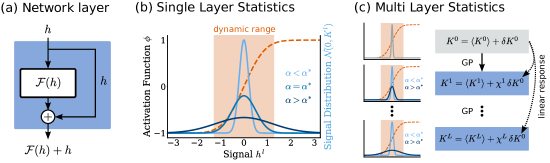
Figure 1: Signal distribution in residual network. (a) Network layer with residual branch and skip connection. The residual branch returns $h\mapsto\mathcal{F}(h)$, the layer passes on $\mathcal{F}(h)+h$ to the next layer. (b) Distribution of the signal $h^{l}$ after layer $l$ (solid curves) relative to the dynamic range $\mathcal{V}$ (shaded orange area) of the activation function $\phi=\text{erf}$ (dashed curve). The signal is Gaussian distributed $h^{l}\sim\mathcal{N}(0,K^{l})$ with variance given by $K^{l}$, which depends on the residual scaling parameter $\alpha$. For values larger than the optimal scaling $\alpha>\alpha^{\ast}$, part of the signal is lost in the saturation of the activation function $\phi$ (dark blue). For values smaller than the optimal scaling $\alpha<\alpha^{\ast}$, the signal is restricted to a small fraction of the dynamic range (light blue) in which the activation function is typically linear. For optimal scaling $\alpha=\alpha^{\ast}$, the signal optimally utilizes the whole dynamic range $\mathcal{V}$ of the activation function $\phi$ (blue). (c) The response function $\chi^{l}$ describes how the variance $K^{l}$, corresponding to the diagonal element of the GP kernel, changes to linear order in the perturbation of the input kernel $\delta K^{0}$ around its data mean $\langle K^{0}\rangle$. The kernel $K^{l}$ of the signal distribution can only increase across layers due to the skip connections; its rate of increase is governed by the residual scaling parameter $\alpha$. If the signal goes into saturation ($\alpha>\alpha^{\ast}$) or remains close to zero ($\alpha<\alpha^{\ast}$), then the overall response of the network output to a change of the input kernel is limited.

We here study the following network model

$$h^{0} =W^{\text{in}}x+b^{\text{in}}\,,$$

$$h^{l} =h^{l-1}+\alpha\left[W^{l}\phi(h^{l-1})+b^{l}\right]\quad l=1,\dots,L,$$ (1)

$$y =W^{\text{out}}\phi(h^{L})+b^{\text{out}}\,,$$

yielding a mapping from the input $x\in\mathbb{R}^{d_{\text{in}}}$ to the output $y\in\mathbb{R}^{d_{\text{out}}}$ as $x\mapsto f(x;\theta)=y$ with network parameters $\theta=\left\{W^{\text{in}},\,b^{\text{in}},\,W^{l},\,b^{l},\,W^{\text{out}},\,b^{\text{out}}\right\}$. Similar to state-of-the-art models such as ResNet-50 [8], the model contains a linear readin and a fully-connected readout layer. Thereby, the input $x\in\mathbb{R}^{d_{\text{in}}}$ of dimension $d_{\text{in}}$, the signal $h^{l}\in\mathbb{R}^{N}$ in layer $l$ of size $N$, and the output $y\in\mathbb{R}^{d_{\text{out}}}$ of dimension $d_{\text{out}}$ can have different dimensions. We refer to the residual branch $\mathcal{F}(h^{l-1})=\alpha\left[W^{l}\phi(h^{l-1})+b^{l}\right]$ together with the skip connection $h^{l-1}$ in (1) as a network layer with index $l$ (see Figure 1(a)). The total number of layers is given by $L$. We assume the non-linear activation function $\phi$ to be saturating and twice differentiable almost everywhere; two common choices satisfying both conditions are the logistic function and the error function. In the following we use $\phi=\text{erf}.$ The residual branch is multiplied by a scaling factor $\alpha$, which is referred to as the residual scaling parameter in the following. We study networks at initialization and thus assume that the network parameters are Gaussian distributed $W_{ij}^{\text{in}}\overset{\text{i.i.d.}}{\sim}\mathcal{N}(0,\sigma_{w,\,\text{in}}^{2}/d_{\text{in}}),\;b_{i}^{\text{in}}\overset{\text{i.i.d.}}{\sim}\mathcal{N}(0,\sigma_{b,\,\text{in}}^{2}),\;$$W_{ij}^{l}\overset{\text{i.i.d.}}{\sim}\mathcal{N}(0,\sigma_{w}^{2}/N),\;b_{i}^{l}\overset{\text{i.i.d.}}{\sim}\mathcal{N}(0,\sigma_{b}^{2}),\;W_{ij}^{\text{out}}\overset{\text{i.i.d.}}{\sim}\mathcal{N}(0,\sigma_{w,\,\text{out}}^{2}/N)$, and $b_{i}^{\text{out}}\overset{\text{i.i.d.}}{\sim}\mathcal{N}(0,\sigma_{b,\,\text{out}}^{2})$.

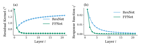
Figure 2: Residual kernels $\bar{C}^{l}$ (a) and the respective response function $\eta^{l}$ (b) in ResNets (blue) compared to FFNets (green). In (a) error bars indicate standard error of the mean obtained from simulation over $10^{3}$ network initializations, solid curves show theory values (2). In (b) dots represent simulations over $10^{2}$ input samples and $10^{3}$ network initializations, solid curves show theory values (4). Errors are of order $10^{-5}$ and therefore not shown. ResNets exhibit a slower decay over layers $l$ compared to FFNets. Other parameters: $\sigma_{w,\,\text{in}}^{2}=\sigma_{w}^{2}=\sigma_{w,\,\text{out}}^{2}=1.2,\,\sigma_{b,\,\text{in}}^{2}=\sigma_{b}^{2}=\sigma_{b,\,\text{out}}^{2}=0.2,\,d_{\text{in}}=d_{\text{out}}=100,\,N=500,\,\alpha=1$.

In this work we study the sensitivity of signal propagation to different inputs. We build on the Gaussian process (GP) result for ResNets [10, 24, 2]: The residual $\mathcal{F}(h^{l})=h^{l}-h^{l-1}$ for $1\leq l\leq L$ becomes Gaussian distributed for infinitely wide networks ($N\rightarrow\infty)$ with variance (see Supplementary Material A for a self-contained derivation of the $N\to\infty$ limit as well as the leading order finite $N$ corrections)

$$\bar{C}^{l} =\alpha^{2}\sigma_{w}^{2}\,\langle\phi(h^{l-1})\phi(h^{l-1})\rangle_{h^{l-1}\sim\mathcal{N}(0,K^{l-1})}+\alpha^{2}\sigma_{b}^{2}\quad 1\leq l\leq L,$$ (2)

where $\bar{C}^{0}=\frac{\sigma_{w,\,\text{in}}^{2}}{d_{\text{in}}}x^{\top}x+\sigma_{b,\,\text{in}}^{2}$ and $K^{l-1}=\sum_{k=0}^{l-1}\bar{C}^{k}$ is the variance of the signal $h^{l-1}$ of layer $l-1$. For brevity, we set $K^{0}\coloneqq\bar{C}^{0}$ and refer to $\bar{C}^{l}$ as the ’residual kernel’ and to $K^{l}$ as ’kernel’. Note that the full kernels including covariances across different inputs can be derived with similar methods as in Supplementary Material A; $K^{l}$ is usually referred to as the GP kernel [14, 10, 24]. Since skip connections just pass on the signal across layers, the variances of the residual branch and the skip connections simply add up under the assumption of i.i.d. distributed network parameters $\theta$ such that the kernel $K^{l-1}$ is the sum of the residual kernels $\bar{C}^{k}$ of all previous layers (for a formal derivation, see Supplementary Material A). More precisely, taking into account the readin and readout layers, the signal $h^{l}$ is Gaussian distributed with

$$K^{l} =\begin{cases}\frac{\sigma_{w,\,\text{in}}^{2}}{d_{\text{in}}}x^{\top}x+\sigma_{b,\,\text{in}}^{2}&l=0\,,\\ \sum_{k=0}^{l}\bar{C}^{k}&1\leq l\leq L\,,\\ \sigma_{w,\,\text{out}}^{2}\langle\phi(h^{L})\phi(h^{L})\rangle_{h^{L}\sim\mathcal{N}(0,K^{L})}+\sigma_{b,\,\text{out}}^{2}&l=L+1\,.\end{cases}$$ (3)

Here $x^{\top}x=\sum_{i=1}^{d_{\text{in}}}x_{i}x_{i}$ denotes the scalar product over input dimensions and $K^{L+1}$ is the kernel of the network output $y$. The recursive formulation for the GP kernel commonly used in previous works [10, 24, 2] can be recovered as $K^{l}=K^{l-1}+\bar{C}^{l}$ for $1\leq l\leq L$.

We are interested in how the signal in deeper layers changes when changing the input from $x$ to $x+\delta x$. This leads to a change of the input kernel $K^{0}=\frac{\sigma_{w,\,\text{in}}^{2}}{d}(x+\delta x)^{\top}(x+\delta x)+\sigma_{b,\,\text{in}}^{2}$. Since we are interested in the scaling of the parameters in the intermediate part of the network, excluding the input parameters $(W^{\text{in}},\,b^{\text{in}})$, it is sufficient to study the signal propagation of the input kernel $K^{0}+\delta K^{0}$. The measure of interest is the response function that describes how the kernel $K^{l}$ of a later network layer changes as a result of a perturbation in the input kernel. In that sense, it is a measure of the network’s sensitivity to different inputs. For simplicity, we here consider perturbations around the average $\langle K^{0}\rangle$ over the data distribution: $K^{0}=\langle K^{0}\rangle+\delta K^{0}$.

Main result of the theoretical framework.

The response function $\eta^{l}$ of the residual $\mathcal{F}(h^{l})=h^{l}-h^{l-1}$ is given by $\displaystyle\eta^{l}$ $\displaystyle=\delta_{l0}+1_{l>0}\,\alpha^{2}\sigma_{w}^{2}\langle\phi^{\prime}(h^{l-1})^{2}+\phi^{\prime\prime}(h^{l-1})\phi(h^{l-1})\rangle_{h^{l-1}\sim\mathcal{N}(0,K^{l-1})}\,\sum_{k=0}^{l-1}\,\eta^{k}\,,$ (4) where $1_{l>0}$ denotes the indicator function such that the second term contributes only for $l>0$. The response function of the signal $h^{l}$ in (1) is then given by the summed residual responses $\chi^{l}=\sum_{k=0}^{l}\,\eta^{k}$. The overall response of the network output amounts to $\displaystyle\chi^{\text{out}}$ $\displaystyle=\sigma_{w,\,\text{out}}^{2}\langle\phi^{\prime}(h^{L})^{2}+\phi^{\prime\prime}(h^{L})\phi(h^{L})\rangle_{h^{L}\sim\mathcal{N}(0,K^{L})}\,\sum_{k=0}^{L}\,\eta^{k}\,.$ (5)

This result, that formally arises as the first-order approximation in $\mathcal{O}\left(N^{-1}\right)$ from a systematic field-theoretic calculation (see Supplementary Material A), can be intuitively understood by linear response arguments: To linear order in the perturbation $\delta K^{0}$, we have the residual kernel $\bar{C}^{l}=\bar{C}^{l}\rvert_{\langle K^{0}\rangle}+\frac{\partial C^{l}}{\partial K^{0}}\rvert_{\langle K^{0}\rangle}\,\delta K^{0}+\mathcal{O}\left(\delta^{2}\right)$, yielding for the response

$$\eta^{l} =\frac{\partial C^{l}}{\partial K^{0}}\rvert_{\langle K^{0}\rangle}=\alpha^{2}\sigma_{w}^{2}\frac{\partial}{\partial K^{l-1}}\langle\phi(h^{l-1})\phi(h^{l-1})\rangle_{h^{l-1}\sim\mathcal{N}(0,K^{l-1})}\,\frac{\partial K^{l-1}}{\partial K^{0}}\rvert_{\langle K^{0}\rangle},$$

and then rewriting $\frac{\partial}{\partial K^{l-1}}\langle\phi(h^{l-1})\phi(h^{l-1})\rangle_{h^{l-1}\sim\mathcal{N}(0,K^{l-1})}=\langle\phi^{\prime}(h^{l-1})^{2}+\phi^{\prime\prime}(h^{l-1})\phi(h^{l-1})\rangle_{h^{l-1}\sim\mathcal{N}(0,K^{l-1})}$ with help of Price’s theorem [17] and $\frac{\partial K^{l-1}}{\partial K^{0}}\rvert_{\langle K^{0}\rangle}=\sum_{k=0}^{l-1}\frac{\partial C^{k}}{\partial K^{0}}\rvert_{\langle K^{0}\rangle}=\sum_{k=0}^{l-1}\eta^{k}$ by the chain rule. The latter expectation value measures how the perturbation of the kernel $K^{l-1}$ affects the residual kernel $\bar{C}^{l}$ in layer $l$. It gets multiplied by the accumulated perturbations of all previous layers, as one expects intuitively due to the skip connections in residual networks. The expression for the response of the kernels $K^{l}$ follows directly from its definition $\chi^{l}=\frac{\partial K^{l}}{\partial K^{0}}\rvert_{\langle K^{0}\rangle}=\frac{\partial}{\partial K^{0}}\sum_{k=0}^{l}\bar{C}^{k}\rvert_{\langle K^{0}\rangle}=\sum_{k=0}^{l}\eta^{l}$. Note that the field-theoretic formalism (see Supplementary Material A) formally shows that this linear response approximation is the $\mathcal{O}\left(N^{-1}\right)$ finite-size correction to the GP result. The framework furthermore allows treating higher-order corrections in a systematic way. For feed-forward and recurrent networks this has been done in Segadlo et al. (2022).

In Figure 2 we compare the behavior of the residual kernels $\bar{C}^{l}$ and the response function $\eta^{l}$ between FFNets and ResNets. While $\bar{C}^{l}$ in FFNets decays to zero as a function of depth, it approaches a value larger than zero in ResNets due to accumulation of variance across layers. Similarly, while the response function in FFNets decays exponentially to zero, it decays much slower in ResNets and approaches zero only asymptotically (see Supplementary Material C.1). The latter observation matches previous results by Yang & Schoenholz (2017) based on the convergence rate of the kernels. In contrast, we here derive the response function that explicitly measures the dependence on the input kernel.

Next, we study the effect of the residual scaling parameter $\alpha$ on the kernels $K^{l}$ and response function $\chi^{l}$ of layer $l$ as those describe the distribution of the signal $h^{l}$. Since $\alpha^{2}$ scales the residual kernels $\bar{C}^{l}$ in (2) that are being summed to obtain $K^{l}$, the residual scaling governs the rate of increase of $K^{l}$ across layers (see Figure 3(a)). The response function $\chi^{l}$ exhibits the same scaling and thus behavior (see Figure 3(b)).

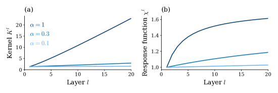
Figure 3: Dependence of kernels $K^{l}$ (a) and the respective response function $\chi^{l}$ (b) on residual scaling parameter $\alpha$. The residual scaling takes values $\alpha\in[1.0,\,0.3,\,0.1]$ (from dark to light blue). It governs the rate of increase in both quantities. Other parameters: $\sigma_{w,\,\text{in}}^{2}=\sigma_{w}^{2}=\sigma_{w,\,\text{out}}^{2}=1.2,\,\sigma_{b,\,\text{in}}^{2}=\sigma_{b}^{2}=\sigma_{b,\,\text{out}}^{2}=0.2,\,d_{\text{in}}=d_{\text{out}}=100,\,N=500$.

3 Optimal scaling of residual branch

Given the strong dependence of the response function on the residual scaling parameter in Figure 3, we study whether an optimal scaling value $\alpha^{\ast}$ exists that maximizes the output response $\chi^{\text{out}}$. Good signal propagation is linked to improved trainability and thus higher generalization performance of trained networks [19, 25].

In Figure 4(a), we indeed see that the output response $\chi^{\text{out}}$ has a maximum for a particular residual scaling $\alpha^{\ast}$. The shape of the response function and thus the optimal value $\alpha^{\ast}$ depend on the network depth $L$, shifting to smaller values $\alpha^{\ast}$ with greater depth. However, we observe an antagonistic effect: the depth dependence becomes weaker for deeper networks. The optimal value $\alpha^{\ast}$ lies between $[0.1,\,0.3]$, as found empirically in previous works [23].

Due to the recursive nature of the non-linear Eqs. (4)-(5) for the response function, we cannot determine the optimal value $\alpha^{\ast}$ analytically. However, we can discern the mechanism behind the signal propagation from (3): For deeper networks the kernels $K^{l}$ grow continuously, so that the signal $h^{l}$ leaves the dynamic range $\mathcal{V}$ of the activation function $\phi$. In consequence, part of the signal $h^{L}$ is lost in the readout layer, reducing the output response $\chi^{\text{out}}$ to varying inputs. The magnitude of the kernels $K^{l}$ depends on $\alpha^{2}$, so that smaller residual scalings lead to a smaller growth of the kernels $K^{l}$ and keep the signal $h^{L}$ in the dynamic range $\mathcal{V}$. For very small scalings $\alpha$, the contribution of the residual branch is suppressed and the network reduces to a single layer perceptron.

Based on this intuition, we derive a theory for the optimal scaling $\alpha^{\ast}$: We assume that the signal $h^{l}$ stays in the dynamic range $\mathcal{V}$ of the activation function so that $\phi(h^{l})\approx h^{l}$. The residual kernel then simplifies to $\bar{C}^{l}=\alpha^{2}\sigma_{w}^{2}\sum_{k=0}^{l-1}\bar{C}^{k}+\alpha^{2}\sigma_{b}^{2}$ and hence $\bar{C}^{l}=\bar{C}^{l-1}+\alpha^{2}\sigma_{w}^{2}\bar{C}^{l-1}$. Solving this recursion, we get $\bar{C}^{l}=(1+\alpha^{2}\sigma_{w}^{2})^{l-1}\,(\alpha^{2}\sigma_{w}^{2}K^{0}+\alpha^{2}\sigma_{b}^{2})$. Using the sum of the first $L+1$ terms of the geometric series and $\bar{C}^{0}=K^{0}$ per definition, we obtain

$$K^{\text{L}} =\sum_{k=0}^{L}\bar{C}^{k}$$ (6)

$$=(1+\alpha^{2}\sigma_{w}^{2})^{L}K^{0}+\frac{\sigma_{b}^{2}}{\sigma_{w}^{2}}\left((1+\alpha^{2}\sigma_{w}^{2})^{L}-1\right)\,.$$ (7)

Assuming the $1\sigma$ range of the distribution to stay within the dynamic range $\mathcal{V}$ for a point-symmetric activation function $\phi$, we set $\mathcal{V}/2\overset{!}{=}\sqrt{K^{L}}$ to obtain an expression for the optimal scaling parameter.

Main result on optimal scaling.

The optimal scaling parameter is approximately given by $$\alpha^{\ast}\approx\frac{1}{\sigma_{w}}\sqrt{\left(\frac{\sigma_{w}^{2}\left(\nicefrac{{\mathcal{V}}}{{2}}\right)^{2}+\sigma_{b}^{2}}{\sigma_{w}^{2}K^{0}+\sigma_{b}^{2}}\right)^{\frac{1}{L}}-1}\,.$$ (8)

For the error function we estimate $\mathcal{V}\approx 1$. Even though this expression builds on certain assumption, it yields a good approximation for the optimal values $\alpha^{\ast}$ in Figure 4(a), as shown in Figure 4(b).

Based on its derivation, this expression however cannot fully capture the behavior of the signal when it reaches the non-linear part of the activation-function. Note that this is solely a limitation of our ansatz for the optimal scaling; the response function itself captures non-linear effects within the network. Further, the assumption $\mathcal{V}/2\overset{!}{=}\sqrt{K^{L}}$ is only an estimate; multiple $\sigma$ ranges could be required for optimal signal propagation. Nevertheless, (8) provides a useful approximation to study scaling properties as its universality across hyperparameters, which we discuss in the next section. Alternatively, we derive this condition from a maximum entropy argument for the signal distribution (see Supplementary Material B). A similar maximum entropy argument has been used by Bukva et al. (2023) to study trainability of feed-forward networks.

Previous works have empirically determined optimal scaling values [28] and their dependence on the network depth $L$ [6, 7, 27]. In contrast, we here obtain an explicit expression for the optimal scaling based on a linear approximation and saturation arguments. The connection between saturation effects and trainability has previously been studied by Bukva et al. (2023), but in feed-forward networks instead of residual networks and based on a maximum-entropy argument instead of using response functions.

3.1 Universality of residual scaling parameter

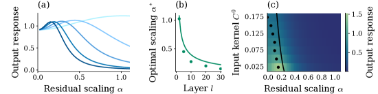
Figure 4: Optimal scaling of residual branch. (a) Output response $\chi^{\text{out}}$ for different depths $L\in[2,\,5,\,10,\,20,\,30]$ (light to dark blue) and input kernel $K^{0}=0.05$. The residual scaling values with largest response concentrate with increasing depth. (b) Optimal residual scaling $\alpha^{\ast}=\mathrm{argmax}(\chi^{\text{out}})$ for input kernel $K^{0}=0.05$. Simulation values (dots) from (a) agree well with theory (8) (curve). (c) Dependence of output response on input kernel $K^{0}$ and residual scaling $\alpha$ at depth $L=30$. The optimal scaling value $\alpha^{\ast}$ (dots indicate simulation, curve indicates theory (8)) decreases for larger input kernels $K^{0}$ due to accumulation of variance across layers. Other parameters: $\sigma_{w}^{2}=1.25\,,\sigma_{b}^{2}=0.05,\,d_{\text{in}}=d_{\text{out}}=100,\,N=500$.

The main strength of the saturation theory (7)-(8) is that it explains the universality of the empirically found range $\alpha^{\ast}\in[0.1,\,0.3]$ [23]. The $L$-th root function dominates the expression in (8), while the dependence on e.g. the dynamic range $\mathcal{V}$ is damped. Therefore, the assumptions made in the previous paragraph have only a small effect on the result. This intuition can be made concrete by writing (8) for large depth $L$ as

$$\alpha^{\ast}\approx\sqrt{\frac{1}{L}}\sqrt{\frac{1}{\sigma_{w}^{2}}\log\left(\frac{\sigma_{w}^{2}\left(\nicefrac{{\mathcal{V}}}{{2}}\right)^{2}+\sigma_{b}^{2}}{\sigma_{w}^{2}K^{0}+\sigma_{b}^{2}}\right)}+\mathcal{O}\left(L^{-1}\right)\,.$$ (9)

Furthermore, the optimal scaling $\alpha^{\ast}$ depends on the ratio between the dynamic range $\left(\nicefrac{{\mathcal{V}}}{{2}}\right)^{2}$ and the input kernel $K^{0}$. For large input kernels $K^{0}$ relative to the dynamic range $\mathcal{V}$, the signal moves into the saturating regime after a few layers. Thus, optimal signal propagation necessitates a smaller residual scaling $\alpha^{\ast}$ (see Figure 4(c)).

Expression (9) recovers the proportionality of the optimal scaling value with $\propto 1/\sqrt{L}$ reported in earlier works [6, 7, 27]. While this expression is valid at great depth $L$ as is common for state-of-the-art architectures, (8) yields a good approximation also for shallower networks. Furthermore, our framework allows us to analyze the dependence on the other hyperparameters.

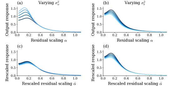
Figure 5: Universality of optimal scaling. (a) Output response $\chi^{\text{out}}$ for varying weight variance $\sigma_{w}^{2}\in[1.0,\,1.25,\,1.5,\,1.75,\,2.0]$ (dark to light) and fixed $\sigma_{b}^{2}=0.05$. (b) Output response $\chi^{\text{out}}$ for varying bias variance $\sigma_{b}^{2}\in[0.05,\,0.06,\,0.07,\,0.08,\,0.09,\,0.1]$ (dark to light) and fixed $\sigma_{b}^{2}=1.75$. (c) Rescaled residual parameter $\hat{\alpha}=\alpha\,\sigma_{w}$ and rescaled response $\hat{\chi}^{\text{out}}=\chi^{\text{out}}/\sigma_{w,\,\text{out}}^{2}$. The curves collapse, showing how the output response depends on an effective parameter scale. (d) Rescaled residual parameter $\hat{\alpha}=\alpha\,\alpha^{\ast}(\sigma_{b,\,\text{ref}})/\alpha^{\ast}(\sigma_{b})$ and output response $\chi^{\text{out}}$. While the maxima coincide, the saturation theory for the optimal scaling cannot capture the dependence of the output response $\chi^{\text{out}}$ on the bias variance $\sigma_{b}^{2}$. Other parameters: $K^{0}=0.05,\,d_{\text{in}}=d_{\text{out}}=100,\,N=500,\,L=30$.

We study the effect of weight variance $\sigma_{w}^{2}$ and bias variance $\sigma_{b}^{2}$ at initialization. While the shape of the output response $\chi^{\text{out}}$ changes noticeably when varying both parameters, the optimal scaling $\alpha^{\ast}$ shows only a weak dependence (Figure 5(a)-(b)) as expected from (8). By computing an estimate of the response function based on the linearized expression (7) as $\partial K^{L+1}/\partial K^{0}=\sigma_{w,\,\text{out}}^{2}\,(1+\alpha^{2}\sigma_{w}^{2})^{L}$, we rescale the residual scaling as $\hat{\alpha}=\alpha\,\sigma_{w}$ and the response function as $\hat{\chi}^{\text{out}}=\chi^{\text{out}}/\sigma_{w,\,\text{out}}^{2}$, yielding a universal behavior irrespective of weight variance $\sigma_{w}^{2}$ (Figure 5(c)). Due to the independence of the linearized expression of $\sigma_{b}^{2}$, we rescale the latter based on the optimal value as $\hat{\alpha}=\alpha\,\alpha^{\ast}(\sigma_{b,\,\text{ref}})/\alpha^{\ast}(\sigma_{b})$ (Figure 5(d)). While the full behavior of the output response $\chi^{\text{out}}$ still contains some nontrivial dependence on $\sigma_{b}^{2}$ that would require further analyses of non-linear effects, rescaling based on saturation theory yields a universal optimal effective scaling $\hat{\alpha}^{*}$.

4 Limitations

As discussed in the previous section, the saturation theory yielding the expression for the optimal scaling (8) cannot fully capture effects that occur once the signal $h^{l}$ reaches the non-linear part of the activation function. This results from the approximation of the activation function as linear in the dynamic range. Note that this limitation applies solely to the approximate optimal scaling; the response function itself captures non-linear effects within the network. Further, the relation between signal variance and size of dynamic range is an estimate. However, for deep networks (8) depends only weakly on the latter choice. Overall, despite being an approximation, the optimal scalings predicted by the saturation theory match well and are able to explain the universality of the value range found by Szegedy et al. (2017).

Further, we here focus on the case of a single data sample. For multiple data samples, the full kernel can be computed straightforwardly using the field-theoretic framework in Supplementary Material A. For the covariances across data samples, the expression in (4) changes slightly $\eta^{l}\propto\langle\phi^{\prime}(h^{l-1})^{2}\rangle_{h^{l-1}\sim\mathcal{N}(0,K^{l-1})}$; the structural properties of the expression remain the same. The optimal scaling $\alpha^{\ast}(K^{0})$ in 8 also varies only slightly across different $K^{0}$. A simple argument is that the optimal scaling value for the largest $K^{0}$ will continue to be a good value for other smaller $K^{0}$. In practice, we expect a trade-off between smaller between-class similarities and larger within-class similarities (measured by $K^{0}$), leading to some robust optimal scaling $\bar{\alpha}^{\ast}$ not yet captured by the presented theory.

Finally, the presented theory assumes the network parameters $\theta$ to be independently and identically distributed as is the case at network initialization, thus describing the trainability at initialization. Also this assumption describes the network prior in a setting of Bayesian inference. However, there is no guarantee that the results continue to hold during training. Nevertheless, there are good indicators that they may: In the lazy learning regime [4], the network parameters change only slightly, remaining close to the network initialization. In the feature learning regime, a recent study showed for feed-forward and convolutional networks that the signal continues to be Gaussian but with kernels adapted to the data [21]. A change of the signal variance can be mapped back to a change of the weight and bias variance, which can be well captured by the presented theory.

5 Conclusion

Understanding signal propagation in neural networks is essential for a theory of trainability and generalization. Regarding these points, residual networks have shown to be superior to feed-forward network [8, 9]; scaling the residual branches in ResNets further amplifies this effect [23]. We here derive the response function of residual networks, a measure for the network’s sensitivity to variability in the input. We show that, in contrast to feed-forward networks, the response function decays to zero only asymptotically, consequently allowing information to propagate to very deep layers in line with Yang & Schoenholz (2017). Further, we show that signal propagation in ResNets is optimal when the signal distribution utilizes the whole dynamic range of the activation function. Beyond this range, information is lost due to saturation effects. We relate the width of the signal distribution to the scaling parameter of the residual branch, allowing us to identify the optimal scaling parameter; an open question until now. Finally, we are able to explain the universality of empirically found optimal values. Thereby, this work sheds light on the interplay between signal propagation, saturation effects and signal scales in residual networks. Furthermore, the field-theoretic framework in the Supplementary Material allows computing finite-size properties of residual networks. We leave this point for future work.

Supplementary Material

Appendix A Field theoretical approach to ResNets

We here calculate the network prior $p(y|x)$ for the residual network model defined in Eq. (1). This derivation uses the same approach as employed in Segadlo et al. (2022) to study deep feed-forward and recurrent networks. The network prior is defined as the probability of an output $y$ given an input $x$ marginalized over the distribution of network parameters $\theta$

$$p(y|x)=\int\mathrm{d}\theta\,p(y|x,\theta)\,p(\theta).$$ (S1)

Given fixed network parameters $\theta$, the probability $p(y|x,\theta)$ is given by enforcing the network model with Dirac $\delta$-distributions as

$$p(y|x,\theta) =\int\mathrm{d}h^{0}\dots\int\mathrm{d}h^{L}\,\delta(y-W^{\text{out}}\phi(h^{L})-b^{\text{out}})$$

$$\qquad\qquad\times\delta(h^{l}-h^{l-1}-\alpha W^{l}\phi(h^{l-1})-\alpha b^{l})$$ (S2)

$$\qquad\qquad\times\delta(h^{0}-W^{\text{in}}x-b^{\text{in}}).$$

A.1 Marginalization over network parameters

The marginalization over the network parameters is given by

$$p(y|x) =\int\mathrm{d}h^{0}\dots\int\mathrm{d}h^{L}\,\langle\delta(y-W^{\text{out}}\phi(h^{L})-b^{\text{out}})\rangle_{\left\{W^{\text{out}},\,b^{\text{out}}\right\}}$$

$$\qquad\qquad\times\langle\delta(h^{l}-h^{l-1}-\alpha W^{l}\phi(h^{l-1})-\alpha b^{l})\rangle_{\left\{W^{l},\,b^{l}\right\}}$$ (S3)

$$\qquad\qquad\times\langle\delta(h^{0}-W^{\text{in}}x-b^{\text{in}})\rangle_{\left\{W^{\text{in}},\,b^{\text{in}}\right\}},$$

where $\left\langle\right\rangle_{\{W,b\}}$ refers to the expectation value over the statistics of weights $W$ and biases $b$. We rewrite the Dirac $\delta$-distributions using the Fourier representation

$$\delta(h)=\int\mathrm{d}\tilde{h}\,\exp\big{(}\tilde{h}^{\mathsf{T}}h\big{)}$$ (S4)

with scalar product $\tilde{h}^{\mathsf{T}}h=\sum_{i=1}^{N}\tilde{h}_{i}h_{i}$, integration measure $\int\mathrm{d}\tilde{h}=\prod_{k}\int_{i\mathbb{R}}\frac{\mathrm{d}\tilde{h}_{k}}{2\pi i}$ and $\tilde{h}$ the conjugate variable to $h$. This yields

$$p(y|x) =\int\mathrm{d}\tilde{y}\int\mathcal{D}\tilde{h}\int\mathcal{D}h\,\left\langle\exp\Big{(}\tilde{y}^{\mathsf{T}}(y-W^{\text{out}}\phi(h^{L})-b^{\text{out}})\Big{)}\right\rangle_{\left\{W^{\text{out}},\,b^{\text{out}}\right\}}$$

$$\qquad\qquad\times\left\langle\exp\Big{(}\big{(}\tilde{h}^{l}\big{)}^{\mathsf{T}}(h^{l}-h^{l-1}-\alpha W^{l}\phi(h^{l-1})-\alpha b^{l})\Big{)}\right\rangle_{\left\{W^{l},\,b^{l}\right\}}$$ (S5)

$$\qquad\qquad\times\left\langle\exp\Big{(}\big{(}\tilde{h}^{0}\big{)}^{\mathsf{T}}(h^{0}-W^{\text{in}}x-b^{\text{in}})\Big{)}\right\rangle_{\left\{W^{\text{in}},\,b^{\text{in}}\right\}},$$

where we write $\int\mathcal{D}h=\prod_{l=0}^{L}\int\mathrm{d}h^{l}$ and $\int\mathcal{D}\tilde{h}=\prod_{l=0}^{L}\int\mathrm{d}\tilde{h}^{l}$ for brevity. Since the network parameters $\theta$ are independently distributed, the integrals decouple and only integrals of the form $\int\mathrm{d}\theta_{k}\,p(\theta_{k})\,\exp\big{(}z\theta_{k}\big{)}$ appear, which can be solved exactly for $\theta_{k}\sim\mathcal{N}(0,\sigma^{2})$ yielding $\exp\big{(}\frac{1}{2}\sigma^{2}z^{2}\big{)}$.

We rewrite the resulting terms as $\sum_{mn}\left[\tilde{y}_{m}\phi(h_{n}^{L})\right]^{2}=\tilde{y}^{\mathsf{T}}\tilde{y\,}\phi(h^{L})^{\mathsf{T}}\phi(h^{L})^{\mathsf{T}}$ and thus get

$$p(y|x) =\int\mathrm{d}\tilde{y}\int\mathcal{D}\tilde{h}\int\mathcal{D}h\,\exp\left(\tilde{y}^{\mathsf{T}}y+\frac{1}{2}\frac{\sigma_{w,\,\text{out}}^{2}}{N}\,\tilde{y}^{\mathsf{T}}\tilde{y}\,\phi(h^{L})^{\mathsf{T}}\phi(h^{L})+\frac{1}{2}\sigma_{b,\,\text{out}}^{2}\tilde{y}^{\mathsf{T}}\tilde{y}\right)$$

$$\qquad\qquad\qquad\times\exp\left(\sum_{l=1}^{L}\left[\tilde{h}^{l}\right]^{\mathsf{T}}\left[h^{l}-h^{l-1}\right]\right)$$

$$\qquad\qquad\qquad\times\exp\left(\sum_{l=1}^{L}\left(\frac{1}{2}\alpha^{2}\frac{\sigma_{w}^{2}}{N}\,\left[\tilde{h}^{l}\right]^{\mathsf{T}}\tilde{h}^{l}\,\phi(h^{l-1})^{\mathsf{T}}\phi(h^{l-1})+\frac{1}{2}\alpha^{2}\sigma_{b}^{2}\left[\tilde{h}^{l}\right]^{\mathsf{T}}\tilde{h}^{l}\right)\right)$$

$$\qquad\qquad\qquad\times\exp\left(\left[\tilde{h}^{0}\right]^{\mathsf{T}}h^{0}+\frac{1}{2}\frac{\sigma_{w,\,\text{in}}^{2}}{d_{\text{in}}}\,\left[\tilde{h}^{0}\right]^{\mathsf{T}}\tilde{h}^{0}\,x{}^{\mathsf{T}}x+\frac{1}{2}\sigma_{b,\,\text{in}}^{2}\left[\tilde{h}^{0}\right]^{\mathsf{T}}\tilde{h}^{0}\right)$$

$$\eqqcolon\int\mathrm{d}\tilde{y}\int\mathcal{D}\tilde{h}\int\mathcal{D}h\,\exp\left(\mathcal{S}(y,\tilde{y},h,\tilde{h}|x)\right).$$

The exponent $\mathcal{S}$ of the integrand, commonly called the action, is given by

$$\mathcal{S}(y,\tilde{y},h,\tilde{h}|x) =\mathcal{S}_{\text{in}}(h^{0},\tilde{h}^{0}|x)+\mathcal{S}_{\text{net}}(h,\tilde{h})+\mathcal{S}_{\text{out}}(y,\tilde{y}|h^{L}),$$ (S6)

where we distinguish between the readin layer

$$\mathcal{S}_{\text{in}}(h^{0},\tilde{h}^{0}|x)\coloneqq\left[\tilde{h}^{0}\right]^{\mathsf{T}}h^{0}+\frac{1}{2}\frac{\sigma_{w,\,\text{in}}^{2}}{d_{\text{in}}}\,\left[\tilde{h}^{0}\right]^{\mathsf{T}}\tilde{h}^{0}\,x{}^{\mathsf{T}}x+\frac{1}{2}\sigma_{b,\,\text{in}}^{2}\left[\tilde{h}^{0}\right]^{\mathsf{T}}\tilde{h}^{0},$$ (S7)

the inner layers of the network with residual connectivity

$$\mathcal{S}_{\text{net}}(h,\tilde{h})\coloneqq\sum_{l=1}^{L}\left[\tilde{h}^{l}\right]^{\mathsf{T}}\left[h^{l}-h^{l-1}\right]+\frac{1}{2}\alpha^{2}\frac{\sigma_{w}^{2}}{N}\,\left[\tilde{h}^{l}\right]^{\mathsf{T}}\tilde{h}^{l}\,\phi(h^{l-1})^{\mathsf{T}}\phi(h^{l-1})+\frac{1}{2}\alpha^{2}\sigma_{b}^{2}\left[\tilde{h}^{l}\right]^{\mathsf{T}}\tilde{h}^{l},$$ (S8)

and the readout layer

$$\mathcal{S}_{\text{out}}(y,\tilde{y}|h^{L})\coloneqq\tilde{y}^{\mathsf{T}}y+\frac{1}{2}\frac{\sigma_{w,\,\text{out}}^{2}}{N}\,\tilde{y}^{\mathsf{T}}\tilde{y}\,\phi(h^{L})^{\mathsf{T}}\phi(h^{L})+\frac{1}{2}\sigma_{b,\,\text{out}}^{2}\tilde{y}^{\mathsf{T}}\tilde{y}.$$ (S9)

In contrast to feed-forward networks, the conjugate variable $\tilde{h}^{l}$ of layer $l$ does not only couple to the signal $h^{l}$ of layer $l$, but also to the signal $h^{l-1}$ of the previous layer $l-1$. This coupling across layers results from the skip connections in residual networks. The interdependence between layers induced by the coupling prohibits the marginalization over the intermediate signals $h^{l}$ in a forward manner as in feed-forward networks.

A.2 Auxiliary variables

Quadratic terms in $h$ and $\tilde{h}$ can be solved as Gaussian integrals. However, in (S7)-(S9) terms proportional to $\propto\left[\tilde{h}^{l}\right]^{\mathsf{T}}\tilde{h}^{l}\,\phi(h^{l-1})^{\mathsf{T}}\phi(h^{l-1})$ appear, which are at least quartic in $h$ and $\tilde{h}$. To treat these terms, we introduce auxiliary variables

$$C^{l} \coloneqq\begin{cases}\frac{\sigma_{w,\,\text{in}}^{2}}{d_{\text{in}}}x{}^{\mathsf{T}}x+\sigma_{b,\,\text{in}}^{2}&l=0,\\ \alpha^{2}\frac{\sigma_{w}^{2}}{N}\phi(h^{l-1})^{\mathsf{T}}\phi(h^{l-1})+\alpha^{2}\sigma_{b}^{2}&1\leq l\leq L,\\ \frac{\sigma_{w,\,\text{out}}^{2}}{N}\phi(h^{L})^{\mathsf{T}}\phi(h^{L})+\sigma_{b,\,\text{out}}^{2}&l=L+1.\end{cases}$$

For wide networks ($N\gg 1$), we expect the empirical average $\frac{1}{N}\sum_{i=1}^{N}\phi(h_{i}^{l-1})^{2}$ to concentrate around its mean value. Based on this intuition, we aim to rewrite the network prior $p(y|x)$ in terms of these scalar variables.

We enforce these definitions with Dirac $\delta$-distributions as in (S2), yielding

$$p(y|x) =\int\mathrm{d}\tilde{y}\int\mathcal{D}\tilde{h}\int\mathcal{D}h\int\mathcal{D}C\int\mathcal{D}\tilde{C}\,\exp\left(\tilde{y}^{\mathsf{T}}y+\frac{1}{2}C^{L+1}\tilde{y}^{\mathsf{T}}\tilde{y}\right)$$

$$\qquad\qquad\qquad\times\exp\left(\sum_{l=1}^{L}\left[\left[\tilde{h}^{l}\right]^{\mathsf{T}}\left[h^{l}-h^{l-1}\right]+\frac{1}{2}C^{l}\left[\tilde{h}^{l}\right]^{\mathsf{T}}\tilde{h}^{l}\right]\right)$$

$$\qquad\qquad\qquad\times\exp\left(\left[\tilde{h}^{0}\right]^{\mathsf{T}}h^{0}+\frac{1}{2}C^{0}\left[\tilde{h}^{0}\right]^{\mathsf{T}}\tilde{h}^{0}\right)$$

$$\qquad\qquad\qquad\times\exp\left(-N\sum_{l=0}^{L+1}\nu_{l}\,C^{l}\,\tilde{C}^{l}+\alpha^{2}\sigma_{w}^{2}\,\sum_{l=1}^{L}\tilde{C}^{l}\phi(h^{l-1})^{\mathsf{T}}\phi(h^{l-1})+N\alpha^{2}\sigma_{b}^{2}\sum_{l=1}^{L}\tilde{C}^{l}\right)$$

$$\qquad\qquad\qquad\times\exp\left(\sigma_{w,\,\text{out}}^{2}\tilde{C}^{L+1}\phi(h^{L})^{\mathsf{T}}\phi(h^{L})+N\sigma_{b,\,\text{out}}^{2}\tilde{C}^{L+1}\right)$$

$$\qquad\qquad\qquad\times\exp\left(\sigma_{w,\,\text{in}}^{2}\tilde{C}^{0}x{}^{\mathsf{T}}x+d_{\text{in}}\sigma_{b,\,\text{in}}^{2}\tilde{C}^{0}\right),$$

where $\int\mathcal{D}C=\prod_{l=0}^{L+1}\int_{\mathbb{R}}\mathrm{d}C^{l}$ and $\int\mathcal{D}\tilde{C}=\prod_{l=0}^{L+1}\int_{i\mathbb{R}}\frac{\mathrm{d}\tilde{C}^{l}}{2\pi i}$ and $\nu_{l}=1+\delta_{0l}\,(d_{\text{in}}/N-1)$ .

Since the scalar variables $C$ and $\tilde{C}$ only couple to sums of $\tilde{h}$ and $\phi(h)$ over all neuron indices, all components of $h$ and $\tilde{h}$ are identically distributed and we can rewrite the expression as

$$p(y|x) =\int\mathrm{d}\tilde{y}\int\mathcal{D}\tilde{h}\int\mathcal{D}h\int\mathcal{D}C\int\mathcal{D}\tilde{C}\,\exp\left(\tilde{y}^{\mathsf{T}}y+\frac{1}{2}C^{L+1}\tilde{y}^{\mathsf{T}}\tilde{y}\right)$$

$$\qquad\qquad\qquad\times\exp\left(N\sum_{l=1}^{L}\left[\tilde{h}^{l}\left[h^{l}-h^{l-1}\right]+\frac{1}{2}C^{l}\left[\tilde{h}^{l}\right]^{2}\right]\right)$$

$$\qquad\qquad\qquad\times\exp\left(N\left[\tilde{h}^{0}h^{0}+\frac{1}{2}C^{0}\left[\tilde{h}^{0}\right]^{2}\right]\right)$$

$$\qquad\qquad\qquad\times\exp\left(-N\sum_{l=0}^{L+1}\nu_{l}\,C^{l}\,\tilde{C}^{l}+N\alpha^{2}\sigma_{w}^{2}\,\sum_{l=1}^{L}\tilde{C}^{l}\phi(h^{l-1})\phi(h^{l-1})+N\alpha^{2}\sigma_{b}^{2}\sum_{l=1}^{L}\tilde{C}^{l}\right)$$

$$\qquad\qquad\qquad\times\exp\left(N\sigma_{w,\,\text{out}}^{2}\tilde{C}^{L+1}\phi(h^{L})\phi(h^{L})+N\sigma_{b,\,\text{out}}^{2}\tilde{C}^{L+1}\right)$$

$$\qquad\qquad\qquad\times\exp\left(\sigma_{w,\,\text{in}}^{2}\tilde{C}^{0}x{}^{\mathsf{T}}x+d_{\text{in}}\sigma_{b,\,\text{in}}^{2}\tilde{C}^{0}\right),$$

where $h^{l}$ and $\tilde{h}^{l}$ now refer to scalar quantities. We move the integrals over the variables $h$ and $\tilde{h}$ to the exponent and reorder the terms as

$$p(y|x) =\int\mathrm{d}\tilde{y}\int\mathcal{D}C\int\mathcal{D}\tilde{C}\,\exp\left(\tilde{y}^{\mathsf{T}}y+\frac{1}{2}C^{L+1}\tilde{y}^{\mathsf{T}}\tilde{y}\right)$$

$$\qquad\qquad\qquad\times\exp\left(-N\sum_{l=0}^{L+1}\nu_{l}\,C^{l}\,\tilde{C}^{l}\right)$$

$$\qquad\times\exp\Bigg{[}N\ln\prod_{l=1}^{L}\int\mathrm{d}h^{l}\int\mathrm{d}\tilde{h}^{l}\,\exp\left(\tilde{h}^{l}\left[h^{l}-h^{l-1}\right]+\frac{1}{2}C^{l}\left[\tilde{h}^{l}\right]^{2}\right)$$

$$\qquad\qquad\qquad\>\times\exp\left(\alpha^{2}\sigma_{w}^{2}\tilde{C}^{l}\,\phi(h^{l-1})\phi(h^{l-1})+\alpha^{2}\sigma_{b}^{2}\sum_{l=1}^{L}\tilde{C}^{l}\right)$$

$$\qquad\qquad\qquad\>\times\exp\left(\sigma_{w,\,\text{out}}^{2}\tilde{C}^{L+1}\phi(h^{L})\phi(h^{L})+\sigma_{b,\,\text{out}}^{2}\tilde{C}^{L+1}\right)$$

$$\qquad\qquad\qquad\>\times\int\mathrm{d}h^{0}\int\mathrm{d}\tilde{h}^{0}\exp\left(\tilde{h}^{0}h^{0}+\frac{1}{2}C^{0}\left[\tilde{h}^{0}\right]^{2}\right)$$

$$\qquad\qquad\qquad\qquad\qquad\qquad\qquad\times\exp\left(\frac{\sigma_{w,\,\text{in}}^{2}}{N}\tilde{C}^{0}x{}^{\mathsf{T}}x+\nu_{0}\sigma_{b,\,\text{in}}^{2}\tilde{C}^{0}\right)\Bigg{]}$$

$$=\int\mathrm{d}\tilde{y}\left\langle\exp\left(\tilde{y}^{\mathsf{T}}y+\frac{1}{2}C^{L+1}\tilde{y}^{\mathsf{T}}\tilde{y}\right)\right\rangle_{C,\tilde{C}},$$

where the auxiliary variables are distributed as $(C,\tilde{C})\sim\exp\big{(}\mathcal{S}_{\text{aux}}(C,\tilde{C})\big{)}$ with

$$\mathcal{S}_{\text{aux}}(C,\tilde{C}) \coloneqq-N\sum_{l=0}^{L+1}\nu_{l}\,C^{l}\,\tilde{C}^{l}+N\mathcal{W}_{\text{aux}}(\tilde{C}|C),$$

$$\mathcal{W}_{\text{aux}}(\tilde{C}|C) \coloneqq\ln\prod_{l=1}^{L}\int\mathrm{d}h^{l}\int\mathrm{d}\tilde{h}^{l}\,\exp\left(\tilde{h}^{l}\left[h^{l}-h^{l-1}\right]+\frac{1}{2}C^{l}\left[\tilde{h}^{l}\right]^{2}\right)$$

$$\qquad\qquad\times\exp\left(\alpha^{2}\sigma_{w}^{2}\tilde{C}^{l}\,\phi(h^{l-1})\phi(h^{l-1})+\alpha^{2}\sigma_{b}^{2}\sum_{l=1}^{L}\tilde{C}^{l}\right)$$

$$\qquad\qquad\times\exp\left(\sigma_{w,\,\text{out}}^{2}\tilde{C}^{L+1}\phi(h^{L})\phi(h^{L})+\sigma_{b,\,\text{out}}^{2}\tilde{C}^{L+1}\right)$$

$$\qquad\qquad\qquad\>\times\int\mathrm{d}h^{0}\int\mathrm{d}\tilde{h}^{0}\exp\left(\tilde{h}^{0}h^{0}+\frac{1}{2}C^{0}\left[\tilde{h}^{0}\right]^{2}\right)$$

$$\qquad\qquad\qquad\qquad\qquad\qquad\qquad\times\exp\left(\frac{\sigma_{w,\,\text{in}}^{2}}{N}\tilde{C}^{0}x{}^{\mathsf{T}}x+\nu_{0}\sigma_{b,\,\text{in}}^{2}\tilde{C}^{0}\right)\,.$$

A.3 Saddle-point approximation

The auxiliary action $\mathcal{S}_{\text{aux}}$ scales with the network width $N$. In the limit of infinite width ($N\rightarrow\infty$), we can thus perform a saddle-point approximation to evaluate integrals of the form

$$\int\mathcal{D}C\int\mathcal{D}\tilde{C}\,f(C,\tilde{C})\,\exp\big{(}\mathcal{S}_{\text{aux}}(C,\tilde{C})\big{)}\overset{N\rightarrow\infty}{=}f(\bar{C},\bar{\tilde{C}}),$$

where $\bar{C}$ and $\bar{\tilde{C}}$ are the saddle points of the auxiliary action $\mathcal{S}_{\text{aux}}$.

We compute these using the conditions

$$\frac{\partial\mathcal{S}_{\text{aux}}}{\partial C} \overset{!}{=}0,$$

$$\frac{\partial\mathcal{S}_{\text{aux}}}{\partial\tilde{C}} \overset{!}{=}0,$$

and get

$$\bar{C}^{l} =\begin{cases}\frac{\sigma_{w,\,\text{in}}^{2}}{d_{\text{in}}}x^{\mathsf{T}}x+\sigma_{b,\,\text{in}}^{2}&l=0,\\ \alpha^{2}\sigma_{w}^{2}\langle\phi(h^{l-1})\phi(h^{l-1})\rangle_{p}+\alpha^{2}\sigma_{b}^{2}&1\leq l\leq L,\\ \sigma_{w,\,\text{out}}^{2}\langle\phi(h^{L})\phi(h^{L})\rangle_{p}+\sigma_{b,\,\text{out}}^{2}&l=L+1,\end{cases}$$

$$\bar{\tilde{C}}^{l} =0\qquad l=0,\dots,L+1,$$

where

$$\langle\dots\rangle_{p} =\prod_{l=1}^{L}\int\mathrm{d}h^{l}\int\mathrm{d}\tilde{h}^{l}\,\dots\,\exp\left(\tilde{h}^{l}\left[h^{l}-h^{l-1}\right]+\frac{1}{2}\bar{C}^{l}\left[\tilde{h}^{l}\right]^{2}\right)$$

$$\qquad\qquad\times\int\mathrm{d}h^{0}\int\mathrm{d}\tilde{h}^{0}\exp\left(\tilde{h}^{0}h^{0}+\frac{1}{2}\bar{C}^{0}\left[\tilde{h}^{0}\right]^{2}\right).$$

For brevity, we also include $\bar{C}^{0}=C^{0}$ here. The average is computed self-consistently with respect to $\bar{C}^{l}$.

By using the residual $f^{l}=h^{l}-h^{l-1}$ for $1\leq l\leq L$, we rewrite the appearing average as

$$\langle\dots\rangle_{p} =\prod_{l=1}^{L}\int\mathrm{d}f^{l}\int\mathrm{d}\tilde{h}^{l}\,\dots\,\exp\left(\tilde{h}^{l}f^{l}+\frac{1}{2}\bar{C}^{l}\left[\tilde{h}^{l}\right]^{2}\right)$$ (S10)

$$\qquad\qquad\times\int\mathrm{d}h^{0}\int\mathrm{d}\tilde{h}^{0}\exp\left(\tilde{h}^{0}h^{0}+\frac{1}{2}\bar{C}^{0}\left[\tilde{h}^{0}\right]^{2}\right)$$

$$=\prod_{l=1}^{L}\int\mathrm{d}f^{l}\,\dots\,\frac{1}{\sqrt{2\pi\bar{C}^{l}}}\exp\left(-\frac{1}{2}\left[\bar{C}^{l}\right]^{-1}\left[f^{l}\right]^{2}\right)$$

$$\qquad\qquad\times\int\mathrm{d}h^{0}\frac{1}{\sqrt{2\pi\bar{C}^{0}}}\exp\left(-\frac{1}{2}\left[\bar{C}^{0}\right]^{-1}\left[h^{0}\right]^{2}\right).$$

From the latter expression follows that the residuals $f^{l}$ for $1\leq l\leq L$ and $h^{0}$ are Gaussian distributed with covariance $\bar{C}^{l}\mathbb{I}$ in the saddle-point approximation. Since the residuals $f^{l}$ are independent Gaussians, the signal $h^{l}$ is also Gaussian distributed with covariance $K^{l}\mathbb{I}=\sum_{k=0}^{l}\bar{C}^{k}\mathbb{I}$.

Thus, we obtain the result in Eq. (3) in the main text

$$\bar{C}^{l} =\alpha^{2}\sigma_{w}^{2}\langle\phi(h^{l-1})\phi(h^{l-1})\rangle_{h^{l-1}\sim\mathcal{N}(0,K^{l-1})}+\alpha^{2}\sigma_{b}^{2},\,\mathrm{for}\,1\leq l\leq L,$$

$$K^{l} =\begin{cases}\frac{\sigma_{w,\,\text{in}}^{2}}{d_{\text{in}}}x^{\mathsf{T}}x+\sigma_{b,\,\text{in}}^{2}&l=0,\\ \sum_{k=0}^{l}\bar{C}^{k}&1\leq l\leq L,\\ \sigma_{w,\,\text{out}}^{2}\langle\phi(h^{L})\phi(h^{L})\rangle_{h^{L}\sim\mathcal{N}(0,K^{L})}+\sigma_{b,\,\text{out}}^{2}&l=L+1.\end{cases}$$

We recover the known GP result for the diagonal kernel entries as $K^{l}=K^{l-1}+\bar{C}^{l}$ [10, 24, 2].

A.4 Next-to-leading order correction

We compute corrections to the saddle-point approximation above. For finite-size networks, the residual kernels $C^{l}$ fluctuate around the above saddle-point value. In lowest-order approximation, we describes these fluctuations as Gaussian. We obtain these by computing the Hessian of the action at the saddle point. Hence, all following averages are with respect to the measure $\langle\dots\rangle_{p}$ defined in (S10). The diagonal terms are given by

$$\frac{\partial^{2}}{\partial C^{l}\partial C^{k}}\mathcal{S}_{\text{aux}} =0\,,$$

$$\frac{\partial^{2}}{\partial\tilde{C}^{l}\partial\tilde{C}^{k}}\mathcal{S}_{\text{aux}} =N\sigma_{w}^{4}\,1_{l>0}1_{k>0}\,\langle\phi(h^{l-1})\phi(h^{l-1}),\phi(h^{k-1})\phi(h^{k-1})\rangle_{c,p}$$

$$\qquad\qquad\times\begin{cases}\alpha^{4}&k,l\neq L+1,\\ \alpha^{2}&k\neq l=L+1\vee l\neq k=L+1,\\ 1&\text{else},\end{cases}$$

where $1_{l>0}$ denotes the indicator function and we denote by $\langle\dots\rangle_{c}$ connected correlations defined as

$$\langle\phi(h^{l-1})\phi(h^{l-1}),\phi(h^{k-1})\phi(h^{k-1})\rangle_{c,p} =\langle\phi(h^{l-1})\phi(h^{l-1})\phi(h^{k-1})\phi(h^{k-1})\rangle_{p}$$

$$\qquad-\langle\phi(h^{l-1})\phi(h^{l-1})\rangle_{p}\,\langle\phi(h^{k-1})\phi(h^{k-1})\rangle_{p}.$$

For the off-diagonal terms, we have

$$\frac{\partial^{2}}{\partial C^{l}\partial\tilde{C}^{k}}\mathcal{S}_{\text{aux}} =-N\nu_{l}\delta_{kl}+N\,1_{k>0}\,\sigma_{w}^{2}\frac{\partial}{\partial C^{l}}\langle\phi(h^{k-1})^{2}\rangle_{h^{k-1}\sim\mathcal{N}(0,K^{k-1})}$$

$$\qquad\qquad\qquad\qquad\times\begin{cases}\alpha^{2}&k\leq L\\ 1&k=L+1\end{cases}$$

$$=-N\nu_{l}\delta_{kl}+N\,1_{k>0}\,\sigma_{w}^{2}\frac{\partial}{\partial K^{k-1}}\langle\phi(h^{k-1})^{2}\rangle_{h^{k-1}\sim\mathcal{N}(0,K^{k-1})}\,\frac{\partial}{\partial C^{l}}K^{k-1}$$

$$\qquad\qquad\qquad\qquad\times\begin{cases}\alpha^{2}&k\leq L\\ 1&k=L+1\end{cases}$$

$$=-N\nu_{l}\delta_{kl}+N\,1_{k>0}\,\sigma_{w}^{2}\langle\phi^{\prime}(h^{k-1})^{2}+\phi^{\prime\prime}(h^{k-1})\phi(h^{k-1})\rangle_{h^{k-1}\sim\mathcal{N}(0,K^{k-1})}\,1_{k>l}$$ (S11)

$$\qquad\qquad\qquad\qquad\times\begin{cases}\alpha^{2}&k\leq L\\ 1&k=L+1\end{cases},$$

where we used Price’s theorem from the second to third line. The condition $k>l$ enforced by the indicator function $1_{k>l}$ results from the term $\frac{\partial}{\partial C^{l}}K^{k-1}$, because $K^{k-1}$ only depends on the $C^{l}$ with $l<k$.

Altogether, we get

$$\text{Hess}(\mathcal{S}_{\text{aux}}) =\left(\begin{array}[]{cc}\frac{\partial^{2}}{\partial C^{2}}\mathcal{S}_{\text{aux}}&\frac{\partial^{2}}{\partial C\,\partial\tilde{C}}\mathcal{S}_{\text{aux}}\\ \frac{\partial^{2}}{\partial\tilde{C}\,\partial C}\mathcal{S}_{\text{aux}}&\frac{\partial^{2}}{\partial\tilde{C}^{2}}\mathcal{S}_{\text{aux}}\end{array}\right)$$

$$\eqqcolon\left(\begin{array}[]{cc}\mathcal{S}_{11}&\mathcal{S}_{12}\\ \mathcal{S}_{21}&\mathcal{S}_{22}\end{array}\right).$$

We obtain the Gaussian fluctuations of the fields $C^{l}$ and $\tilde{C}^{l}$ by taking the negative inverse of the Hessian, also called the propagator in field theory

$$\Delta =-\text{Hess}(\mathcal{S}_{\text{aux}})^{-1}$$

$$\eqqcolon\left(\begin{array}[]{cc}\Delta_{11}&\Delta_{12}\\ \Delta_{21}&\Delta_{22}\end{array}\right).$$

By using the block structure and the fact that $\mathcal{S}_{11}=0$, we have

$$\Delta_{11} =\Delta_{12}\,\mathcal{S}_{22}\,\Delta_{21},$$ (S12)

$$\Delta_{12} =-\mathcal{S}_{21}^{-1},$$ (S13)

$$\Delta_{22} =0.$$ (S14)

Since the off-diagonal block matrix $\mathcal{S}_{21}$ is a lower triangular matrix, its inverse can be computed using forward propagation

$$\Delta_{12}^{lm} =N^{-1}\nu_{l}^{-1}\delta_{lm}+H(l)\,\sigma_{w}^{2}\langle\phi^{\prime}(h^{l-1})^{2}+\phi^{\prime\prime}(h^{l-1})\phi(h^{l-1}\rangle_{h^{l-1}\sim\mathcal{N}(0,K^{l-1})}\,\sum_{k=0}^{l-1}\Delta_{12}^{km}$$

$$\qquad\qquad\qquad\qquad\times\begin{cases}\alpha^{2}&k\leq L\\ 1&k=L+1\end{cases}.$$

A.5 Response function

The propagator $\Delta$ gives the covariances of the fields $C^{l}$ and $\tilde{C}^{l}$ as

$$\left(\begin{array}[]{cc}\Delta_{11}&\Delta_{12}\\ \Delta_{21}&\Delta_{22}\end{array}\right)=\left(\begin{array}[]{cc}\text{Cov}(C,C)&\text{Cov}(C,\tilde{C})\\ \text{Cov}(\tilde{C},C)&\text{Cov}(\tilde{C},\tilde{C})\end{array}\right).$$

Since the auxiliary fields $\tilde{C}^{l}$ represent changes in the fields $C^{l}$, the off-diagonal term $\Delta_{12}^{lm}=\text{Cov}\left(C^{l},\tilde{C}^{m}\right)$ can be understood as the response of the network residual in layer $l$ to a perturbation of the residual in layer $m$. Due to the network architecture, any response can only propagate forward in the network, which is reflected in the term $1_{k>l}$ in (S11).

For signal propagation it is most relevant how varying inputs $x$, leading to varying input kernels $K^{0}$, are propagated through the network. This corresponds to $\Delta_{12}^{l0}$. In the main text, we refer to this quantity as the response function $\eta^{l}$. Here, we derive it as a $\mathcal{O}(N^{-1})$ correction to the NNGP result.

A.6 Comparison to feed-forward networks

Segadlo et al. (2022) study the following feed-forward architecture

$$h^{0} =W^{\text{in}}x+b^{\text{in}},$$

$$h^{l} =W^{l}\phi(h^{l-1})+b^{l}\quad l=1,\dots,L,$$ (S15)

$$y =W^{\text{out}}\phi(h^{L})+b^{\text{out}}.$$

In comparison, the network model considered here adds skip connections as well as a scaling $\alpha$ of the residual branch. For direct comparisons, we can set the latter to $\alpha=1$.

In contrast to the results for FFNets, the kernel $K^{l}$ in layer $l$ depends explicitly not only on the kernel of the previous layer but on all preceding layers (see [20] Section 4.1). This property directly results from the skip connections in residual networks. Thereby, the response function in layer $l$ retains information from all preceding layers, such that information can propagate to deeper network layers as shown in Fig. 2. Accordingly, the variances $\Delta_{11}$ of the fields $C^{l}$ in (S12) also yield different values. Since we here focus on properties of the response function, we leave the effect of fluctuations of the fields $C^{l}$ themselves for future work.

Appendix B Maximum entropy condition for optimal scaling

We here derive an alternative condition for optimal signal variance, building on Bukva et al. (2023) who proposed this method to study trainability in feed-forward networks. Their conjecture is that networks with internal signal distributions that are approximately uniform, or put differently maximally entropic, are more expressive.

For wide networks, the signal distribution of internal layers is approximately Gaussian

$$p(h;\sigma^{2})=\frac{1}{\sqrt{2\pi\sigma^{2}}}\exp\left(-\frac{1}{2\sigma^{2}}h^{2}\right),$$

taking only a scalar component here as these are independent of one another.

We here focus on the readout layer. The distribution of the post-activation $z=\phi(h)$ is then

$$p(z;\sigma^{2})=\frac{1}{\sqrt{2\pi\sigma^{2}}\phi^{\prime}(\phi^{-1}(x))}\exp\left(-\frac{1}{2\sigma^{2}}\phi^{-1}(z)^{2}\right).$$

For $\phi=\text{erf}$, the post-activation is bounded by $z\in[-1,1]$. Thus, we compute the Kullback-Leibler divergence between the distribution of the post-activation and a uniform distribution on that interval

$$D_{\text{KL}}(p_{\text{uni}}|p_{\phi}) =\int_{-1}^{1}\mathrm{d}z\,p_{\text{uni}}(z)\,[\ln p_{\text{uni}}(z)-\ln p_{\phi}(z)]$$

$$=\int_{-1}^{1}\mathrm{d}z\,\frac{1}{2}\ln\left(\frac{1}{2}\right)+\frac{1}{2}\frac{1}{2\sigma^{2}}\phi^{-1}(z)^{2}+\frac{1}{2}\ln\left(\sqrt{2\pi}\sigma\phi^{\prime}(\phi^{-1}(z))\right)$$

$$=\ln\left(\frac{1}{2}\right)+\frac{1}{2}\int_{-1}^{1}\mathrm{d}z\,\frac{1}{2\sigma^{2}}\phi^{-1}(z)^{2}+\ln\left(\sqrt{2\pi}\sigma\frac{2}{\sqrt{\pi}}\exp(-\phi^{-1}(z)^{2})\right)$$

$$=\ln\left(\frac{1}{2}\right)+\ln(\sqrt{8}\sigma)+\frac{1}{2}\int_{-1}^{1}\mathrm{d}z\,\left(\frac{1}{2\sigma^{2}}-1\right)\phi^{-1}(z)^{2}$$

$$=\ln\left(\frac{\sqrt{8}}{2}\right)+\ln(\sigma)+\frac{1}{2}\left(\frac{1}{2\sigma^{2}}-1\right)\int_{-\infty}^{\infty}\mathrm{d}h\,\phi^{-1}(\phi(h))^{2}\,\phi^{\prime}(h)$$

$$=\ln\left(\sqrt{2}\right)+\frac{1}{2}\ln(\sigma^{2})+\frac{1}{2}\left(\frac{1}{2\sigma^{2}}-1\right)\int_{-\infty}^{\infty}\mathrm{d}h\,h^{2}\,\frac{2}{\sqrt{\pi}}\exp(-h^{2})$$

$$=\ln\left(\sqrt{2}\right)+\frac{1}{2}\ln(\sigma^{2})+\frac{1}{2}\left(\frac{1}{2\sigma^{2}}-1\right)\int_{-\infty}^{\infty}\mathrm{d}h\,h^{2}\,\frac{1}{\sqrt{2\pi}}\exp(-\frac{1}{2}h^{2})$$

$$=\ln\left(\sqrt{2}\right)+\frac{1}{2}\ln(\sigma^{2})+\frac{1}{2}\left(\frac{1}{2\sigma^{2}}-1\right).$$

Maximizing the Kullback-Leibler divergence between these amounts to

$$0\overset{!}{=}\frac{\partial}{\partial\sigma^{2}}D_{\text{KL}}(p_{\text{uni}}|p_{\phi}) =\frac{1}{\sigma^{2}}-\frac{1}{4}\frac{1}{\sigma^{4}},$$

yielding as the condition for the signal variance before the readout layer

$$\sigma^{2}\overset{!}{=}\frac{1}{4}.$$

This condition is equivalent to the one in the Section 3 under the assumption that the dynamic range of the error function is given by $\mathcal{V}=1$.

Appendix C Additional plots

C.1 Decay of response function

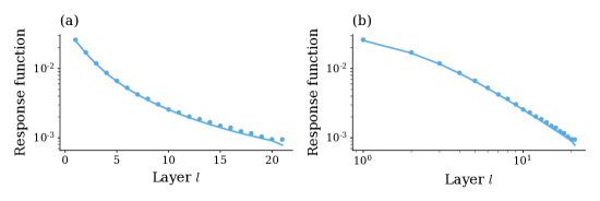
Figure 6: Log-plot (a) and log-log-plot (b) of the response function $\eta^{l}$ for a residual network of depth $L=20$. Dots represent simulations over $10^{2}$ input samples and $10^{3}$ network initializations, solid curves show theory values. The decay of the response function is sub-exponential (a). In later layers, the decay follows a power law (b). Other parameters: $\sigma_{w,\,\text{in}}^{2}=\sigma_{w}^{2}=\sigma_{w,\,\text{out}}^{2}=1.2,\,\sigma_{b,\,\text{in}}^{2}=\sigma_{b}^{2}=\sigma_{b,\,\text{out}}^{2}=0.2,\,d_{\text{in}}=d_{\text{out}}=100,\,N=500,\,\alpha=1$.

References

- Balduzzi et al. [2017] Balduzzi, D., Frean, M., Leary, L., Lewis, J. P., Ma, K. W.-D., & McWilliams, B. (2017). The shattered gradients problem: If resnets are the answer, then what is the question? In D. Precup & Y. W. Teh (Eds.), Proceedings of the 34th International Conference on Machine Learning, Volume 70 of Proceedings of Machine Learning Research, pp. 342–350. PMLR.
- Barzilai et al. [2023] Barzilai, D., Geifman, A., Galun, M., & Basri, R. (2023). A kernel perspective of skip connections in convolutional networks. In The Eleventh International Conference on Learning Representations.
- Bukva et al. [2023] Bukva, A., de Gier, J., Grosvenor, K. T., Jefferson, R., Schalm, K., & Schwander, E. (2023). Criticality versus uniformity in deep neural networks.
- Chizat et al. [2019] Chizat, L., Oyallon, E., & Bach, F. (2019). On Lazy Training in Differentiable Programming. Red Hook, NY, USA: Curran Associates Inc.
- Furusho & Ikeda [2019] Furusho, Y., & Ikeda, K. (2019). Resnet and batch-normalization improve data separability. In W. S. Lee & T. Suzuki (Eds.), Proceedings of The Eleventh Asian Conference on Machine Learning, Volume 101 of Proceedings of Machine Learning Research, pp. 94–108. PMLR.
- Hayou et al. [2021] Hayou, S., Clerico, E., He, B., Deligiannidis, G., Doucet, A., & Rousseau, J. (2021). Stable resnet. In A. Banerjee & K. Fukumizu (Eds.), Proceedings of The 24th International Conference on Artificial Intelligence and Statistics, Volume 130 of Proceedings of Machine Learning Research, pp. 1324–1332. PMLR.
- Hayou et al. [2021] Hayou, S., Ton, J.-F., Doucet, A., & Teh, Y. W. (2021). Robust pruning at initialization. In International Conference on Learning Representations.
- He et al. [2016a] He, K., Zhang, X., Ren, S., & Sun, J. (2016a). Deep residual learning for image recognition. In Proceedings of the IEEE Conference on Computer Vision and Pattern Recognition (CVPR).
- He et al. [2016b] He, K., Zhang, X., Ren, S., & Sun, J. (2016b). Identity mappings in deep residual networks. In European Conference on Computer Vision, Volume 9908, pp. 630–645.
- Huang et al. [2020] Huang, K., Wang, Y., Tao, M., & Zhao, T. (2020). Why do deep residual networks generalize better than deep feedforward networks? — a neural tangent kernel perspective. In H. Larochelle, M. Ranzato, R. Hadsell, M. Balcan, & H. Lin (Eds.), Advances in Neural Information Processing Systems, Volume 33, pp. 2698–2709. Curran Associates, Inc.
- Ioffe & Szegedy [2015] Ioffe, S., & Szegedy, C. (2015). Batch normalization: Accelerating deep network training by reducing internal covariate shift. In Proceedings of the 32nd International Conference on International Conference on Machine Learning - Volume 37, ICML’15, pp. 448–456. JMLR.org.
- Krizhevsky & Hinton [2009] Krizhevsky, A., & Hinton, G. (2009). Learning multiple layers of features from tiny images. Technical report.
- Krizhevsky et al. [2012] Krizhevsky, A., Sutskever, I., & Hinton, G. E. (2012). Imagenet classification with deep convolutional neural networks. In F. Pereira, C. J. C. Burges, L. Bottou, & K. Q. Weinberger (Eds.), Adv. Neural Inf. Process. Syst., Volume 25, pp. 1097–1105. Curran Associates, Inc.
- Lee et al. [2017] Lee, J., Bahri, Y., Novak, R., Schoenholz, S. S., Pennington, J., & Sohl-Dickstein, J. (2017). Deep neural networks as gaussian processes. ArXiv, 1711.00165.
- Li et al. [2016] Li, S., Jiao, J., Han, Y., & Weissman, T. (2016). Demystifying resnet. CoRR abs/1611.01186.
- Ling & Qiu [2019] Ling, Z., & Qiu, R. C. (2019). Spectrum concentration in deep residual learning: A free probability approach. IEEE Access 7, 105212–105223.
- Papoulis & Pillai [2002] Papoulis, A., & Pillai, S. U. (2002). Probability, Random Variables, and Stochastic Processes (4th ed.). Boston: McGraw-Hill.
- Poole et al. [2016] Poole, B., Lahiri, S., Raghu, M., Sohl-Dickstein, J., & Ganguli, S. (2016). Exponential expressivity in deep neural networks through transient chaos. In Advances in Neural Information Processing Systems 29.
- Schoenholz et al. [2017] Schoenholz, S. S., Gilmer, J., Ganguli, S., & Sohl-Dickstein, J. (2017). Deep information propagation. In International Conference on Learning Representations.
- Segadlo et al. [2022] Segadlo, K., Epping, B., van Meegen, A., Dahmen, D., Krämer, M., & Helias, M. (2022). Unified field theoretical approach to deep and recurrent neuronal networks. J. Stat. Mech. Theory Exp. 2022(10), 103401.
- Seroussi et al. [2023] Seroussi, I., Naveh, G., & Ringel, Z. (2023). Separation of scales and a thermodynamic description of feature learning in some cnns. Nature Communications 14(1), 908.
- Silver et al. [2016] Silver, D., Huang, A., Maddison, C. J., Guez, A., Sifre, L., Van Den Driessche, G., Schrittwieser, J., Antonoglou, I., Panneershelvam, V., Lanctot, M., et al. (2016). Mastering the game of go with deep neural networks and tree search. Nature 529(7587), 484–489.
- Szegedy et al. [2017] Szegedy, C., Ioffe, S., Vanhoucke, V., & Alemi, A. A. (2017). Inception-v4, inception-resnet and the impact of residual connections on learning. In Proceedings of the Thirty-First AAAI Conference on Artificial Intelligence, AAAI’17, pp. 4278–4284. AAAI Press.
- Tirer et al. [2022] Tirer, T., Bruna, J., & Giryes, R. (2022). Kernel-based smoothness analysis of residual networks. In J. Bruna, J. Hesthaven, & L. Zdeborova (Eds.), Proceedings of the 2nd Mathematical and Scientific Machine Learning Conference, Volume 145 of Proceedings of Machine Learning Research, pp. 921–954. PMLR.
- Yang & Schoenholz [2017] Yang, G., & Schoenholz, S. (2017). Mean field residual networks: On the edge of chaos. In I. Guyon, U. V. Luxburg, S. Bengio, H. Wallach, R. Fergus, S. Vishwanathan, & R. Garnett (Eds.), Advances in Neural Information Processing Systems, Volume 30. Curran Associates, Inc.
- Zaeemzadeh et al. [2021] Zaeemzadeh, A., Rahnavard, N., & Shah, M. (2021). Norm-preservation: Why residual networks can become extremely deep? IEEE Transactions on Pattern Analysis and Machine Intelligence 43(11), 3980–3990.
- Zhang et al. [2022] Zhang, H., Yu, D., Yi, M., Chen, W., & Liu, T.-Y. (2022). Stabilize deep resnet with a sharp scaling factor . Mach. Learn. 111(9), 3359–3392.
- Zhang et al. [2019] Zhang, J., Han, B., Wynter, L., Low, B. K. H., & Kankanhalli, M. (2019). Towards robust resnet: A small step but a giant leap. In Proceedings of the Twenty-Eighth International Joint Conference on Artificial Intelligence, IJCAI-19, pp. 4285–4291. International Joint Conferences on Artificial Intelligence Organization.