Poisson-Gaussian Holographic
Phase Retrieval
with Score-based Image Prior
Abstract
Phase retrieval (PR) is a crucial problem in many imaging applications. This study focuses on resolving the holographic phase retrieval problem in situations where the measurements are affected by a combination of Poisson and Gaussian noise, which commonly occurs in optical imaging systems. To address this problem, we propose a new algorithm called “AWFS" that uses the accelerated Wirtinger flow (AWF) with a score function as generative prior. Specifically, we formulate the PR problem as an optimization problem that incorporates both data fidelity and regularization terms. We calculate the gradient of the log-likelihood function for PR and determine its corresponding Lipschitz constant. Additionally, we introduce a generative prior in our regularization framework by using score matching to capture information about the gradient of image prior distributions. We provide theoretical analysis that establishes a critical-point convergence guarantee for the proposed algorithm. The results of our simulation experiments on three different datasets show the following: 1) By using the PG likelihood model, the proposed algorithm improves reconstruction compared to algorithms based solely on Gaussian or Poisson likelihood. 2) The proposed score-based image prior method, performs better than the method based on denoising diffusion probabilistic model (DDPM), as well as plug-and-play alternating direction method of multipliers (PnP-ADMM) and regularization by denoising (RED).
I Introduction
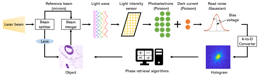
Poisson-Gaussian phase retrieval (PR) is a nonlinear inverse problem, where the goal is to recover a signal from the (square of) magnitude-only measurements that are corrupted by both Poisson and Gaussian noise [1]. This problem is crucial in numerous applications across various fields such as astronomy [2], X-ray crystallography [3], optical imaging [4], Fourier ptychography [5, 6, 7, 8] and coherent diffractive imaging (CDI) [9]. In CDI, a coherent beam source illuminates a sample of interest and a reference. When the beam hits the sample, it generates secondary electromagnetic waves that propagate until they reach a detector. By measuring the photon flux, the detector can capture and record a diffraction pattern. This pattern is roughly proportional to the square of Fourier transform magnitude of electric field associated with the illuminated objects [10, 11]. Recovering the structure of the sample from its diffraction pattern is an non-linear inverse problem known as holographic PR. To solve this problem, the maximum a posterior (MAP) estimate can be conducted with the following form:
| (1) |
where denotes the image to recover, is the measurement collected, denotes the corresponding system matrix in holographic PR where denotes the number of measurements and denotes the dimension of . The known reference image provides additional information to reduce the ambiguity of ; using an extended reference is a common technique in Holographic CDI [12, 13]. Following Bayes’ rule, we denote and as the data-fidelity term and the regularization term, respectively.
In practical scenarios, the measurements are contaminated by both Poisson and Gaussian (PG) noise. The Poisson distribution is due to the photon counting and dark current [14]. The Gaussian statistics stem from the readout structures (e.g., analog-to-digital converter (ADC)) of common cameras. Fig. 1 illustrates the PG mixed noise statistics in the holographic PR.
Because the PG likelihood is complicated (see (4)), most previous works [15, 26, 4, 37, 38, 39, 40, 38, 41, 16, 17, 18, 19, 20, 21, 22, 23, 24, 25, 27, 7, 28, 29, 30, 31, 32, 33, 34, 5, 35, 36] approximate the Poisson noise statistics by the central limit theorem and work with a substitute Gaussian log-likelihood estimate problem; or use the Poisson maximum likelihood model but simply disregards Gaussian readout noise. Besides, other more complicated approximation methods have also been proposed, such as shifted Poisson model [42], the unbiased inverse transformation of a generalized Anscombe transform [43, 8] and the majorize-minimize algorithm [44]. However, these approximate methods can lead to a suboptimal solution after optimization that results in a lower-quality reconstruction.
Apart from the likelihood modeling, the regularizer provides prior information about underlying object characteristics that may aid in resolving ill-posed inverse problems. Beyond simple choices of such as total variation (TV) or the L1-norm of coefficients of wavelet transform [45], deep learning (DL)-integrated algorithms for solving inverse problems in computational imaging have been reported to be the state-of-the-art [46]. The trained networks can be used as an object prior for regularizing the reconstructed image to remain on a learned manifold [47]. Incorporating a trained denoising network as a regularizer led to methods such as plug-and-play (PnP) [48, 49, 50], and regularization by denoising (RED) [51]. In contrast to training a denoiser using clean images, there is growing popularity of self-supervised image denoising approaches that do not require clean data as the training target [52, 53, 54].
In addition to training a denoiser as regularizer, generative model-based priors are also proposed [55, 56]. Recently, diffusion models have gained significant attention for image generation [57, 58, 59, 60]. These probabilistic image generation models start with a clean image and gradually increase the level of noise added to the image, resulting in white Gaussian noise. Then in the reverse process, a neural network is trained to learn the noise in each step to generate or sample a clean image as in the original data distribution. The score-based diffusion models estimate the gradients of data distribution and can be used as plug-and-play priors for the inverse problem solving [61] such as image delurring, MRI and CT reconstruction [62, 63, 64, 65, 66, 67]. However, the realm of using score-based models to perform phase retrieval is relatively unexplored; previous relevant works [68, 61] applied denoising diffusion probabilistic modeling (DDPM) to PR but with less realistic system models and under solely Gaussian or Poisson noise statistics.
In summary, our contribution is in three-fold:
-
•
We present a new algorithm known as accelerated Wirtinger flow with score-based image prior (i.e., in (1)) to address the challenge of Holographic phase retrieval (PR) problem in the presence of Poisson and Gaussian (PG) noise statistics.
-
•
Theoretically, we derive a Lipschitz constant for the Holographic PR’s PG log-likelihood and subsequently demonstrate the critical points convergence guarantee of our proposed algorithm.
-
•
Simulation experiments demonstrate that: 1) Algorithms with the PG likelihood model yield superior reconstructions in comparison to those relying solely on either the Poisson or Gaussian likelihood models. 2) With the proposed score-based prior as regularization, the proposed approach generates higher quality reconstructions and is more robust to variation of noise levels without any parameter tuning, when compared to alternative state-of-the-art methods.
II Background
This section reviews holographical phase retrieval and machine learning-based regularizers for inverse problem solving.
II-A Phase Retrieval (PR)
Gaussian PR. By assuming the elements of follow independent Gaussian distributions , the data fidelity term in (1) becomes . To solve the corresponding MAP optimization problem, a popular method is Wirtinger flow (WF) [23, 37, 38, 39] using the Wirtinger gradient: To determine an appropriate step size for the Wirtinger gradient, one can utilize the Lipschitz constant, or consider using methods such as empirical trial and error, backtracking line search or observed Fisher information [32]. To further accelerate the WF, one can use Nesterov’s momentum methods [69] or optimized gradient methods [70], leading to the accelerated Wirtinge flow (AWF) [7, 71, 72, 73] that is commonly used in solving PR problems. Apart from WF, other methods such as matrix-lifting [15, 26, 4], Gerchberg-Saxton [41], majorize-minimize [40] and alternating direction method of multipliers (ADMM) [20] have also been proposed.
Poisson PR. The Poisson ML model assumes , so that in (1) has the form: Similar to the Gaussian case, one can also apply WF [74] with where and denote element-wise multiplication and division, respectively.
Algorithm 1 summarizes the WF approach for PR. The Gaussian and Poisson models are both suboptimal for practical scenario where the measurements are corrupted with Poisson plus Gaussian noise. Furthermore, many previous works [15, 17, 18, 19, 21, 22, 26, 37, 38, 39, 35, 44, 68, 24, 74] modeled the system matrix (in (1)) as i.i.d. random Gaussian or randomly masked Fourier transform; these assumptions simplify the PR problem and lead to elegant mathematical derivations (e.g., spectral initialization [23, 75]), but they are less related to optical imaging systems used in practical PR [76]. Practical PR involves canonical Fourier transform-based system matrices such as Fresnel PR [77, 78], holographic PR [79], ptychographic PR [80, 81] and Fraunhofer PR [82, 76]. Some previous works also remove the square of the Fourier transform magnitude (see (III-A)) [22, 35, 68, 24]. However, this square of magnitude indicates the amount of wavelength-weighted power emitted by a light source per unit area, so its removal reduces the practicality.
Return
II-B Deep Learning-based Regularizers
PnP and RED. Both PnP and RED are widely adopted in a variety of inverse problems [83, 84, 85, 86]. By implicitly representing the prior in (1) by an image denoiser, plug-and-play (PnP) methods [87, 88] were proposed to allow the integration of the physical measurement models and powerful DL-based denoisers as image priors [50]. The model-agnostic nature of the denoiser allows PnP methods to be applied to multiple imaging problems using a single DL denoiser simply by changing the imaging model. Regularization by denoising (RED) [89, 90] is an algorithm closely related to PnP that uses denoising engine in defining the regularization of the inverse problems.
Score Function and Diffusion Models. Let denote a model for the prior distribution of the latent image ; the score function is then defined as111This definition differs from the score function in statistics where the gradient is taken w.r.t. of . . Consider a sequence of positive noise scales (for white Gaussian ): , with being small enough so that noise of this level does not visibly affect the image, and depending on the application. Score matching can be used to train a noise conditional score network (NCSN) [91, 57] as follows:
| (2) |
With enough data, the neural network is expected to learn the distribution where and is defined in (1). To sample from the prior, the method of Langevin dynamics is frequently used [57].
To leverage diffusion models for solving inverse problems, previous methods generally recast the reconstruction problem as a conditional generation or sampling problem [68, 61, 60, 92, 67, 93]. This involves relying on the capacity of diffusion models to produce high-quality images while complying with data-fidelity constraints. However, in applications where the data collection is costly, i.e., with a limited amount of training data, it is often challenging to obtain a diffusion model that can generate high-quality images even in an unconditional way. With such a scenario, we found that the score function learned during training diffusion models can serve as an effective image prior (as demonstrated in Section IV), which can capture certain data characteristics when trained for the denoising prediction in the reverse process of the diffusion model. Similar to previous works [61] that uses the score function as a PnP prior, here we also incorporate the score function as a regularization in the optimization objective for solving the PR problem. We think this is a more efficient scheme for incorporating diffusion priors especially for applications with a limited amount of training data that is a very common situation in the optical imaging sector.
III Methods
III-A Wirtinger Flow (WF)
Based on the physical model as demonstrated in Fig. 1, we model the system matrix by the (oversampled and scaled) discrete Fourier transform applied to a concatenation of the sample , a blank image (representing the holographic separation condition [30]) and a known reference image , so that follows the following distribution:
| (3) |
Here denotes the mean of background measurements, denotes the variance of Gaussian noise, and denotes a scaling factor (being quantum efficiency, conversion gain, etc) after applying the Fourier transform. Plugging the negative log-likelihood of (III-A) into (1) leads to
| (4) | ||||
Here denotes the length of , denotes the th row of (since is linear). We opt to use WF for estimating because it is commonly used in practice due to its simplicity and efficiency [23]. The WF algorithm is based on the gradient of (4):
| (5) | ||||
Lemma 1. The function is Lipschitz differentiable and the Lipschitz constant for is:
| (6) |
The proof of Lemma 1 is given in [94].
Theorem 1.
Assume is bounded above by for each , a Lipschitz constant of is
| (7) |
where is .
Proof: Let denote a function that maps a vector to a scalar; it is the sum of each over . Let denote a function that maps a vector to the measurement space ; it is the concatenation of each . So , , and .
By the chain rule, the Hessian of is
| (8) |
Assume is bounded above by for each . Then it follows that by the construction of matrix-vector multiplication, leading to a Lipschitz constant for :
|
|
(9) |
Here denotes a Lipschitz constant for , not necessarily the best one. To compute , we substitute the Lipschitz constant of into (5) and apply Lemma 1, leading to
| (10) |
To compute , let
| (11) |
From the fact that by its construction, one can derive that
| (12) | ||||
Theorem 1 is an extension of [94] that considers a linear transformation model to a non-linear transformation () and with a different system matrix .
However, due to the infinite sum in Poisson-Gaussian WF (4), we approximate the following [94]:
| (13) |
with given by
| (14) |
where denotes the Lambert function. The accuracy of this approximation is controlled by . Reference [94] did a comprehensive analysis on the maximum error value of the truncated sum (13) and found the bound was quite precise.
III-B Accelerated Wirtinger Flow with Score-based Image Prior
For the acceleration scheme in the WF algorithm, we followed the implementation of [95] as its convergence guarantee was proved. Under the assumption that the true score function can be learned properly, when we have a trained score function by applying (II-B), the gradient descent algorithm for MAP estimation (1) has the form: . Algorithm 2 summarizes our proposed AWFS algorithm (the vanilla version without acceleration is given in Appendix A-C). In a similar fashion as Langevin dynamics, we choose to be a descending scale of noise levels. In practice, we generally use each noise level a fixed number of times, with geometrically spaced noise levels between some lower and upper bound. The stepsize factor in Algorithm 2 can be selected empirically, but we show that the Lipschitz constant of the gradient exists as demonstrated in Theorem 2 (the proof is given in the Appendix A-B); hence with sufficiently small step size , the sequence generated by Algorithm 2 will converge to a critical point of the posterior distribution in (1).
Lemma 2. The Fourier transform (and inverse transform) of an absolutely integrable function is continuous.
Lemma 3. Suppose a sequence of functions converges in the to some function , and that each is absolutely integrable. Then is also absolutely integrable.
Proposition 1. The derivative of is bounded on the interval .
A brief proof of Proposition 1 can be started by using derivatives of convolution, i.e.,
| (15) |
And then use Lemma 2 and 3 and the fact that a sequence of Gaussian mixture models (GMMs) can be used to approximate any smooth probability distribution in convergence [96, pp. 65]. The complete proof can be found in the appendix.
Lemma 4: Suppose is an everywhere twice differentiable function. Then is bounded if the following three conditions are met:
-
1.
is bounded.
-
2.
itself is bounded below by a positive number and also bounded above.
-
3.
is bounded.
Proposition 2. The gradient of is Lipschitz continuous on .
By the definition of Lipschitz continuity, it suffices to show the Hessian of has bounded entries. By renaming the variables, and redefining , we may consider the boundedness of on and use Lemma 4 to remove the log. The appendix shows the full proof of Proposition 2.
.
Theorem 2.
For a smooth density function that has finite expectation, the Lipschitz constant of exists when each element in satisfy for each j. Furthermore, if the weighting factor is chosen appropriately following [95], i.e., according to whichever higher posterior probability between and ; then with sufficiently small , the sequence generated by Algorithm 2 is bounded, and any accumulation point of is a critical point of the posterior distribution in (1).
Proof: By Proposition 2, and from the design of Algorithm 2, and are both bounded between for all , so the Lipschitz constant of exists. With the stepsize satisfying , and the weighting factor being chosen according to whichever higher posterior probability between and (see [95]), then we satisfy all conditions in Theorem 1 of [95], which establishes the critical-point convergence of Algorithm 2. ∎
Theorem 2 states that is needed to achieve convergence; nevertheless, we empirically discovered that setting also led to promising performance. Compared to our score-based image prior approach, another method is to alternate data-consistency updates with the sampling step of a diffusion model based on denoising diffusion probabilistic models (DDPM) framework [68], as shown in Algorithm 3.
Return .
IV Experiment
IV-A Experiment Settings
Dataset. We tested all algorithms on three dataset: 162 histopathology images related to breast cancer [97] (train/val/test is 122/20/20); 920 images from CelebA dataset [98] (train/val/test is 800/100/20); and 720 images from a homemade CT-density dataset (train/val/test is 600/100/20). The CT-density dataset was generated from SPECT/CT images for Yttrium-90 radionuclide therapy after applying the CT-to-density calibration curve [99]. Although the size of training datasets are relatively small compared to typical datasets such as ImageNet or LSUN [58, 60] that have millions of images, we do not require the score functions to learn image priors strong enough to generate realistic images from white Gaussian noise; rather, it is sufficient for the priors to be able to denoise moderately noisy images.
System Model. The system matrix is based on discrete Fourier transform of the concatenation of the true image , a blank image and a reference image with scaling and oversampling. We set the scaling factor to be in the range so that the average counts per pixel range from 6 to 25; the oversampled ratio is set to 2. We set to be a binary random image similar to what was used in [30]. The standard deviation of the Gaussian read noise added to the measurements was set as .
Implemented Algorithms. For unregularized algorithms, we implemented Gaussian WF, Poisson WF and Poisson-Gaussian WF. For regularized algorithms, we implemented smoothed total variation (TV) based on the Huber function [100, p. 184] and PnP/RED methods with the DnCNN denoiser [101]: PnP-ADMM [87], PnP-PGM [88], and RED-SD [51]. We also implemented the RED-SD algorithm with “Noise2Self" zero-shot image denoising network [53] (RED-SD-SELF). For diffusion-based models, we implemented DOLPH [68] and our proposed AWFS. The Appendix A-C shows the implementation details of each algorithm. We used spectral initialization [75] for the Gaussian PR and Poisson PR methods; we then used the output results from Poisson PR to initialize other algorithms. We ran all algorithms until convergence in normalized root mean squared error (NRMSE) or reached the maximum number of iterations (e.g., 50).
To evaluate the robustness and limitation of these algorithms, we first tuned the parameters for each algorithm at the noise level when and , and then held them fixed throughout all experiments (Table I, Table II, Fig. 5 and Fig. 6). This is because in practice the ground truths are unknown so that it is impossible to tune parameters on each testing data. Though the numbers reported can fluctuate after careful refinement, e.g., by performing grid search on tuning parameters, such techniques would potentially impede the algorithm’s practical use.
Network Training. For PnP denoising networks, we trained all denoisers on different noise levels and found that worked the best on our data. We also used the denoiser scaling technique from [102] to dynamically adjust the performance of all PnP methods. To performing score matching, we applied 20 geometrically spaced noise levels between 0.005 and 0.1 on each of the training images. All networks were implemented in PyTorch and trained on an NVIDIA Quadro RTX 5000 GPU using the ADAM optimizer [103] for 1000 epochs with the best one being selected based off the validation error, i.e., the mean squared error (MSE) loss.
IV-B Results
We compared all implemented algorithms both qualitatively, by visualizing the reconstructed images and residual errors, and quantitatively, by computing the NRMSE and structural similarity index measure (SSIM). Due to the global phase ambiguity, i.e., all the algorithms can recover the signal only to within a constant phase shift due to the loss of global phase information, we corrected the phase of by
| Likelihood | Unregularized (SSIM/NRMSE) | DOLPH (SSIM/NRMSE) | AWFS (SSIM/NRMSE) | |||
| DataSet: Histopathology [97] | ||||||
| Poisson | 0.54 0.18 | 31.7 10.2 | 0.72 0.13 | 19.5 6.1 | 0.83 0.06 | 16.2 3.7 |
| Poisson-Gaussian | 0.57 0.18 | 28.9 9.0 | 0.80 0.06 | 16.0 2.9 | 0.85 0.05 | 15.4 3.7 |
| DataSet: CelebA [98] | ||||||
| Poisson | 0.39 0.10 | 24.5 11.4 | 0.61 0.12 | 15.6 10.6 | 0.72 0.16 | 15.2 11.8 |
| Poisson-Gaussian | 0.42 0.10 | 21.8 9.1 | 0.71 0.11 | 13.7 11.1 | 0.74 0.15 | 14.8 11.9 |
| DataSet: CT-Density | ||||||
| Poisson | 0.19 0.06 | 48.9 13.1 | 0.38 0.11 | 25.6 7.5 | 0.84 0.08 | 17.8 4.3 |
| Poisson-Gaussian | 0.24 0.06 | 40.8 9.5 | 0.55 0.08 | 20.0 3.3 | 0.88 0.05 | 16.4 3.7 |
| Dataset | Histopathology [97] | CelebA [98] | CT-Density | |||
| Methods | SSIM | NRMSE (%) | SSIM | NRMSE (%) | SSIM | NRMSE (%) |
| Unregularized | 0.57 0.18 | 28.9 9.0 | 0.42 0.10 | 21.8 9.1 | 0.24 0.06 | 40.8 9.5 |
| RED-SD-SELF [53] | 0.66 0.13 | 21.9 4.5 | 0.60 0.09 | 15.9 10.6 | 0.34 0.04 | 28.1 4.1 |
| PnP-ADMM [87] | 0.71 0.11 | 20.7 4.2 | 0.56 0.08 | 16.7 8.1 | 0.55 0.03 | 31.2 2.7 |
| TV regularizer | 0.72 0.11 | 18.2 3.9 | 0.64 0.07 | 14.4 8.6 | 0.41 0.03 | 23.7 2.8 |
| RED-SD [51] | 0.76 0.09 | 16.8 3.6 | 0.69 0.11 | 13.9 10.9 | 0.38 0.04 | 25.9 4.0 |
| PnP-PGM [88] | 0.78 0.11 | 16.5 4.5 | 0.74 0.14 | 13.5 11.3 | 0.42 0.07 | 24.6 4.4 |
| DOLPH [68] | 0.80 0.06 | 16.0 2.9 | 0.71 0.11 | 13.7 11.1 | 0.55 0.08 | 20.0 3.3 |
| WFS | 0.76 0.12 | 18.2 5.5 | 0.63 0.16 | 16.9 11.8 | 0.53 0.17 | 21.3 7.6 |
| AWFS (Proposed) | 0.85 0.05 | 15.4 3.7 | 0.74 0.15 | 14.8 11.9 | 0.88 0.05 | 16.4 3.7 |
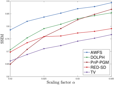
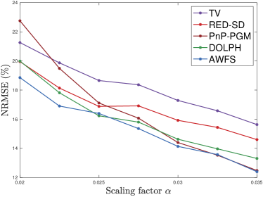
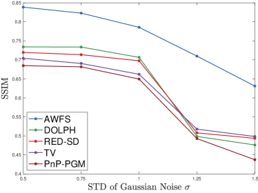
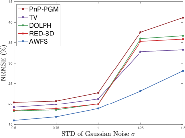
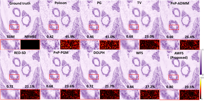
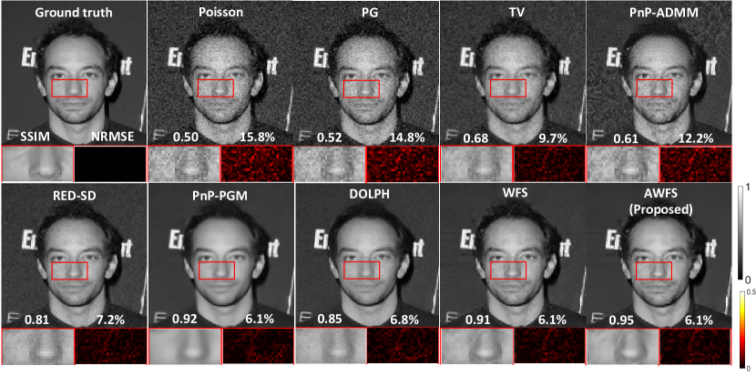
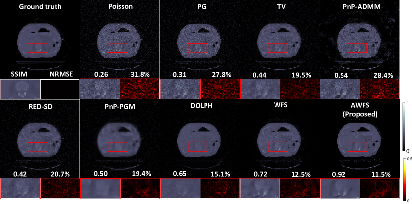
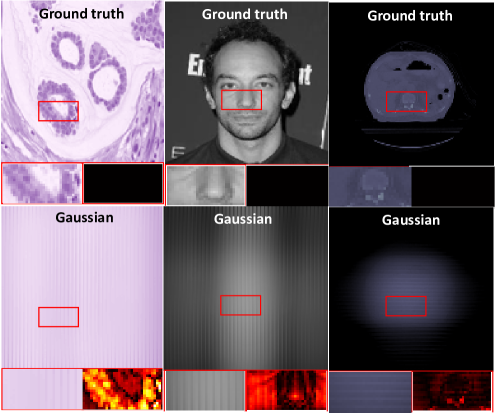
Fig. 2, Fig. 3 and Fig. 4 visualize reconstructed images generated by algorithms mentioned in the previous section. The WF with PG likelihood outperforms WF with Poisson likelihood with consistently a higher SSIM and lower NRMSE. Moreover, we found unregularized Gaussian WF failed to reconstruct similar to what was reported in [40] (examples are shown in the appendix). Of the regularized algorithms with PG likelihood, our proposed AWFS had less visual noise and achieved greater detail recovery compared to other methods, as evidenced by the zoomed-in area in these figures.
For quantitative evaluations, Table I exemplifies the effect of using our proposed PG likelihood as compared to the simpler Poisson likelihoods. We did not run the Gaussian likelihood with DDPM or AWFS due to the abysmal performance with this likelihood. In all cases, usage of the PG likelihood results in improved image quality in terms of both metrics. Table II consists of experiments using the PG likelihood and shows the efficacy of the proposed AWFS method over other methods. In particular, our AWFS had superior quantitative performance over all other compared methods on Histopathology and CT-density dataset; in contrast, the PnP-Prox showed the lowest NRMSE on celebA dataset. This can be due to higher randomness in celebrity faces because the effectiveness of generative models can vary depending on the dataset being used. So when provided with a small amount of training data with high randomness, image denoising models (DnCNN) can possibly more effective than generative models.
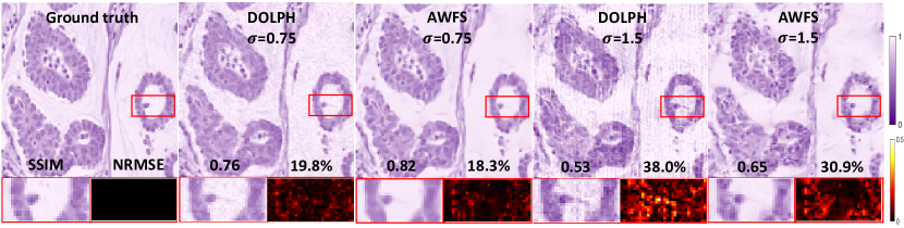
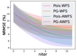
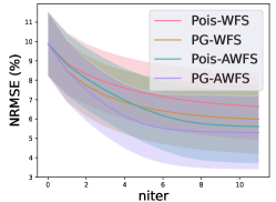
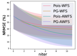
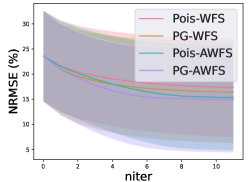
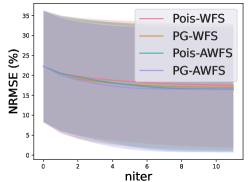
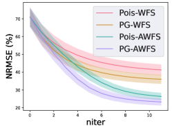
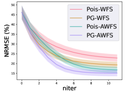
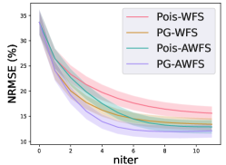
We also tested the robustness of the leading algorithms in Table II, by varying both scaling factor and STD of Gaussian noise . Results are illustrated in Fig. 5 and Fig. 6, where our AWFS algorithm had the highest SSIM and lowest NRMSE. In Fig. 6, AWFS demonstrated minimal variations in SSIM and NRMSE metrics than DOLPH as evidenced by the smaller discrepancies in SSIM (0.17 vs. 0.23) and NRMSE (12.6% vs. 18.2%) when varies from 0.75 to 1.5. Fig. 7 compares the convergence rate of AWF vs. WF for the Poisson and PG likelihood, respectively. Under a variety of noise level, we found the AWF consistently converges faster than WF in terms of number of iterations.

V Discussion
PR has a long-standing history in the field of signal processing and imaging. Pioneering works such as the error reduction (ER) and hybrid input-output (HIO) algorithms by Gerchberg Saxton [41] and Fienup [104] have been proposed to address this problem. These iterative algorithms involve constraints imposed on evaluations between the image domain and frequency domain, however, these methods have limitations in terms of the quality of reconstructed images and their convergence remains uncertain [105]. Another approach to solving PR problems is through compressed sensing and optimization techniques like Wirtinger flow (WF) [23], matrix lifting [15, 26, 4], MM [40] and ADMM [20]. In this paper, we focus on the WF algorithm due to it is straightforward to incorporate with the DL regularizer for the image prior. The likelihood modelling of the noise statistics existing in the measurement is also critical. Previous studies have primarily focused on modelling either Gaussian or Poisson likelihood only, but in practical scenarios, both types of noise are often encountered. Therefore, this paper contributes to a more practical perspective of addressing the holographic PR problem by using a PG likelihood and incorporating state-of-the-art deep learning image priors.
In our evaluation of three datasets, we consistently observed that the use of PG likelihood yielded superior performance compared to using either Poisson or Gaussian likelihood alone. This finding aligns with the natural expectation of accurately modeling the noise likelihood. Additionally, we noted that the results obtained from the CT-density dataset were generally in less quality in comparison to those from the other two datasets. This can be attributed to lower average counts per pixel (plenty of blank pixels near the image boundary).
The use of DL image prior can be considered from two folds: training a denoiser or training to learn the density distribution of images. In our work, we applied both approaches and observed that the effectiveness of these methods differs depending on the dataset tested. Specifically, in the Histopathology dataset [97] and the CT-density dataset, where the images share similar structures, the generative models performs better even trained on limited amount of data. In the case of the CelebA dataset [98], which includes a wide variety of celebrity faces, generative models do not exhibit as strong performance as denoiser methods when trained on limited data. This is likely due to the fact that generating high-quality images is generally more challenging than removing noise from existing images and may necessitate a larger training dataset.
The effectiveness of accelerated WF compared to the vanilla WF is due to the nature of non-convexity of the PR problem. Although recent advances on geometric landscape analysis of PR can guarantee that all local minimizers are global even with random initialization [106], in practice the measurements are contaminated by noise so that perhaps much more measurements are required for the cost function to have a benign geometric landscape.
Despite the promising results achieved with our proposed AWFS approach, there are several limitations of our work. First of all, the approximated calculation of infinite sum in (4), though accurate, is computationally expensive. Therefore, future work should focus on finding ways to accelerate this calculation process while maintaining its accuracy. Secondly, we did not implement and test the accelerated WF applied on the diffusion posterior sampling (DPS) method [93], of which the network is fine-tuned from a pretrained state-of-the-art diffusion model. This approach has the potential to advance current methods in PR problem and we will investigate it in the future.
VI Conclusion
We proposed a novel algorithm based on Accelerated Wirtinger Flow and Score-based image prior (AWFS) for Poisson-Gaussian holographic phase retrieval. With evaluation on simulated experiments, we demonstrated that our proposed AWFS algorithm had the best performance both qualitatively and quantitatively and was more robust to various noise levels, compared to other state-of-the-art methods. Furthermore, we proved that our proposed algorithm has a critical-point convergence guarantee. Therefore, our approach has much promise for translation in real-world applications encountering phase retrieval problems.
References
References
- [1] K. Jaganathan, Y.. Eldar and B. Hassibi “Phase retrieval: an overview of recent developments” https://arxiv.org/abs/1510.07713, 2015
- [2] J. Dainty and James Fienup “Phase retrieval and image reconstruction for astronomy” In Imag. Recov. Theory Appl. 13, 1987, pp. 231–275
- [3] R.. Millane “Phase retrieval in crystallography and optics” In J. Opt. Soc. Am. A 7.3, 1990, pp. 394–411 DOI: 10.1364/JOSAA.7.000394
- [4] Yoav Shechtman, Yonina C Eldar, Oren Cohen, Henry Nicholas Chapman, Jianwei Miao and Mordechai Segev “Phase Retrieval with Application to Optical Imaging: A contemporary overview” In IEEE Sig. Proc. Mag. 32.3 IEEE, 2015, pp. 87–109 DOI: 10.1109/MSP.2014.2352673
- [5] L. Bian, J. Suo, J. Chung, X. Ou, C. Yang, F. Chen and Q. Dai “Fourier ptychographic reconstruction using Poisson maximum likelihood and truncated Wirtinger gradient” In Nature Sci. Rep. 6.1, 2016 DOI: 10.1038/srep27384
- [6] Y. Zhang, P. Song and Q. Dai “Fourier ptychographic microscopy using a generalized Anscombe transform approximation of the mixed Poisson-Gaussian likelihood” In Optics Express 25.1, 2017, pp. 168–79 DOI: 10.1364/OE.25.000168
- [7] Rui Xu, Mahdi Soltanolkotabi, Justin P. Haldar, Walter Unglaub, Joshua Zusman, Anthony F.. Levi and Richard M. Leahy “Accelerated Wirtinger Flow: A fast algorithm for ptychography” http://arxiv.org/abs/1806.05546, 2018 arXiv:1806.05546 [eess.IV]
- [8] X. Tian “Fourier ptychographic reconstruction using mixed Gaussian-Poisson likelihood with total variation regularisation” In Electronics Letters 55.19, 2019, pp. 1041–3 DOI: 10.1049/el.2019.1141
- [9] Tatiana Latychevskaia “Iterative phase retrieval in coherent diffractive imaging: practical issues” In Appl. Opt. 57.25 Optica Publishing Group, 2018, pp. 7187–7197 DOI: 10.1364/AO.57.007187
- [10] David A. Barmherzig, Ju Sun, Emmanuel J. Candes, T.J. Lane and Po-Nan Li “Dual-Reference Design for Holographic Phase Retrieval” In 2019 13th International conference on Sampling Theory and Applications (SampTA), 2019, pp. 1–4 DOI: 10.1109/SampTA45681.2019.9030848
- [11] Ju Barmherzig, Po-Nan Li, T.J. Lane and Emmanuel J. Candès “Holographic phase retrieval and reference design” In Inverse problems 35.9 Ithaca: IOP Publishing, pp. 94001– DOI: 10.1088/1361-6420/ab23d1
- [12] M. Saliba, T. Latychevskaia, J. Longchamp and H. Fink “Fourier Transform Holography: A Lensless Non-Destructive Imaging Technique” In Microsc. Microanal. 18.S2, 2012
- [13] Manuel Guizar-Sicairos and James R. Fienup “Holography with extended reference by autocorrelation linear differential operation” In Opt. Express 15.26 Optica Publishing Group, 2007, pp. 17592–17612 URL: https://opg.optica.org/oe/abstract.cfm?URI=oe-15-26-17592
- [14] Ligong Wang “The Poisson Channel With Varying Dark Current Known to the Transmitter” In IEEE Transactions on Information Theory 65.8, 2019, pp. 4966–4978 DOI: 10.1109/TIT.2019.2911474
- [15] Emmanuel J Candès, Thomas Strohmer and Vladislav Voroninski “PhaseLift: Exact and Stable Signal Recovery from Magnitude Measurements via Convex Programming” In Comm. Pure Appl. Math. 66.8 Hoboken: Wiley Subscription Services, Inc., A Wiley Company, 2013, pp. 1241–1274 DOI: 10.1002/cpa.21432
- [16] Praneeth Netrapalli, Prateek Jain and Sujay Sanghavi “Phase Retrieval Using Alternating Minimization” In IEEE Trans. Sig. Proc. 63.18 IEEE, 2015, pp. 4814–4826 DOI: 10.1109/TSP.2015.2448516
- [17] Irene Waldspurger “Phase Retrieval With Random Gaussian Sensing Vectors by Alternating Projections” In IEEE Trans. Info. Theory 64.5 IEEE, 2018, pp. 3301–3312 DOI: 10.1109/TIT.2018.2800663
- [18] Bing Gao and Zhiqiang Xu “Phaseless Recovery Using the Gauss-Newton Method” In IEEE Trans. Sig. Proc. 65.22 IEEE, 2017, pp. 5885–5896 DOI: 10.1109/TSP.2017.2742981
- [19] Li Ji and Zhou Tie “On gradient descent algorithm for generalized phase retrieval problem” In 2016 IEEE 13th International Conference on Signal Processing (ICSP) IEEE, 2016, pp. 320–325 DOI: 10.1109/ICSP.2016.7877848
- [20] Junli Liang, Petre Stoica, Yang Jing and Jian Li “Phase Retrieval via the Alternating Direction Method of Multipliers” In IEEE Sig. Proc. Letters 25.1, 2018, pp. 5–9 DOI: 10.1109/LSP.2017.2767826
- [21] Yang Yang, Marius Pesavento, Yonina C. Eldar and Björn Ottersten “Parallel Coordinate Descent Algorithms for Sparse Phase Retrieval” In ICASSP 2019 - 2019 IEEE International Conference on Acoustics, Speech and Signal Processing (ICASSP), 2019, pp. 7670–7674 DOI: 10.1109/ICASSP.2019.8683363
- [22] Ju Sun, Qing Qu and John Wright “A geometric analysis of phase retrieval” In 2016 IEEE International Symposium on Information Theory (ISIT), 2016, pp. 2379–2383 DOI: 10.1109/ISIT.2016.7541725
- [23] Emmanuel Candes, Xiaodong Li and Mahdi Soltanolkotabi “Phase Retrieval via Wirtinger Flow: Theory and Algorithms” In IEEE Trans. Info. Theory 61.4, 2015, pp. 1985–2007 DOI: 10.1109/TIT.2015.2399924
- [24] Zihui Wu, Yu Sun, Jiaming Liu and Ulugbek Kamilov “Online Regularization by Denoising with Applications to Phase Retrieval” In 2019 IEEE/CVF International Conference on Computer Vision Workshop (ICCVW), 2019, pp. 3887–3895 DOI: 10.1109/ICCVW.2019.00482
- [25] P. Thibault and M. Guizar-Sicairos “Maximum-likelihood refinement for coherent diffractive imaging” In New J. of Phys. 14.6, 2012, pp. 063004 DOI: 10.1088/1367-2630/14/6/063004
- [26] E.. Candes, Y.. Eldar, T. Strohmer and V. Voroninski “Phase retrieval via matrix completion” In SIAM J. Imaging Sci. 6.1, 2013, pp. 199–225 DOI: 10.1137/110848074
- [27] A. Goy, K. Arthur, S. Li and G. Barbastathis “Low photon count phase retrieval using deep learning” In Phys. Rev. Lett. 121.24, 2018, pp. 243902 DOI: 10.1103/PhysRevLett.121.243902
- [28] David A. Barmherzig and Ju Sun “Low-Photon Holographie Phase Retrieval” In Imaging and Applied Optics Congress Optica Publishing Group, 2020 DOI: 10.1364/COSI.2020.JTu4A.6
- [29] I. Vazquez, I.. Harmon, J… Luna and M. Das “Quantitative phase retrieval with low photon counts using an energy resolving quantum detector” In J. Opt. Soc. Am. A 38.1, 2021, pp. 71–9 DOI: 10.1364/JOSAA.396717
- [30] Hannah Lawrence, David Barmherzig, Henry Li, Michael Eickenberg and Marylou Gabrie “Phase Retrieval with Holography and Untrained Priors: Tackling the Challenges of Low-Photon Nanoscale Imaging” In Proceedings of the 2nd Mathematical and Scientific Machine Learning Conference 145, 2022, pp. 516–567
- [31] Abhiram Gnanasambandam and Stanley H. Chan “Image Classification in the Dark Using Quanta Image Sensors” In Computer Vision – ECCV 2020: 16th European Conference, 2020, pp. 484–501 DOI: 10.1007/978-3-030-58598-3_29
- [32] Zongyu Li, Kenneth Lange and Jeffrey A. Fessler “Poisson Phase Retrieval in Very Low-Count Regimes” In IEEE Transactions on Computational Imaging 8, 2022, pp. 838–850 DOI: 10.1109/TCI.2022.3209936
- [33] Ghania Fatima, Zongyu Li, Aakash Arora and Prabhu Babu “PDMM: A novel Primal-Dual Majorization-Minimization algorithm for Poisson Phase-Retrieval problem” In IEEE Trans. Sig. Proc., 2022, pp. 1–1 DOI: 10.1109/TSP.2022.3156014
- [34] Y. Chen and E.. Candes “Solving random quadratic systems of equations is nearly as easy as solving linear systems” In Comm. Pure Appl. Math. 70.5, 2017, pp. 822–83 DOI: 10.1002/cpa.21638
- [35] H. Zhang, Y. Liang and Y. Chi “A nonconvex approach for phase retrieval: Reshaped Wirtinger flow and incremental algorithms” In J. Mach. Learning Res. 18.141, 2017, pp. 1–35 URL: http://jmlr.org/papers/v18/16-572.html
- [36] Huibin Chang, Yifei Lou, Yuping Duan and Stefano Marchesini “Total variation–based phase retrieval for Poisson noise removal” In SIAM J. Imag. Sci. 11.1 SIAM PUBLICATIONS, 2018, pp. 24–55 DOI: 10.1137/16M1103270
- [37] Xue Jiang, Sreeraman Rajan and Xingzhao Liu “Wirtinger Flow Method With Optimal Stepsize for Phase Retrieval” In IEEE Sig. Proc. Letters 23.11 IEEE, 2016, pp. 1627–1631 DOI: 10.1109/LSP.2016.2611940
- [38] T. Cai, Xiaodong Li and Zongming Ma “Optimal Rates of Convergence for Noisy Sparse Phase Retrieval via Thresholded Wirtinger Flow” In Annals Stat. 44.5 Hayward: Institute of Mathematical Statistics, 2016, pp. 2221–2251 DOI: 10.1214/16-AOS1443
- [39] Mahdi Soltanolkotabi “Structured Signal Recovery From Quadratic Measurements: Breaking Sample Complexity Barriers via Nonconvex Optimization” In IEEE Trans. Info. Theory 65.4 IEEE, 2019, pp. 2374–2400 DOI: 10.1109/TIT.2019.2891653
- [40] T. Qiu, P. Babu and D.. Palomar “PRIME: phase retrieval via majorization-minimization” In IEEE Trans. Sig. Proc. 64.19, 2016, pp. 5174–86 DOI: 10.1109/TSP.2016.2585084
- [41] R.. Gerchberg and W.. Saxton “Practical Algorithm for Determination of Phase from Image and Diffraction Plane Pictures” In OPTIK 35.2, 1972, pp. 237–246
- [42] D.. Snyder, A.. Hammoud and R.. White “Image recovery from data acquired with a charge-coupled-device camera” In J. Opt. Soc. Am. A 10.5, 1993, pp. 1014–23 DOI: 10.1364/JOSAA.10.001014
- [43] Markku Makitalo and Alessandro Foi “Optimal Inversion of the Generalized Anscombe Transformation for Poisson-Gaussian Noise” In IEEE Trans. Imag. Proc. 22.1, 2013, pp. 91–103 DOI: 10.1109/TIP.2012.2202675
- [44] Ghania Fatima and Prabhu Babu “PGPAL: A monotonic iterative algorithm for Phase-Retrieval under the presence of Poisson-Gaussian noise” In IEEE Sig. Proc. Letters, 2022, pp. 1–1 DOI: 10.1109/LSP.2022.3143469
- [45] Ingrid Daubechies “Ten Lectures on Wavelets” Society for IndustrialApplied Mathematics, 1992 DOI: 10.1137/1.9781611970104
- [46] Greg Ongie, Ajil Jalal, Christopher A. Metzler, Richard Baraniuk, Alexandros G. Dimakis and Rebecca M. Willett “Deep Learning Techniques for Inverse Problems in Imaging” In IEEE Journal on Selected Areas in Information Theory 1, 2020, pp. 39–56
- [47] Ashish Bora, Ajil Jalal, Eric Price and Alexandros G. Dimakis “Compressed Sensing using Generative Models” In Proceedings of the 34th International Conference on Machine Learning 70, Proceedings of Machine Learning Research PMLR, 2017, pp. 537–546
- [48] Stanley H. Chan, Xiran Wang and Omar A. Elgendy “Plug-and-Play ADMM for Image Restoration: Fixed-Point Convergence and Applications” In IEEE Transactions on Computational Imaging 3.1, 2017, pp. 84–98 DOI: 10.1109/TCI.2016.2629286
- [49] Kai Zhang, Yawei Li, Wangmeng Zuo, Lei Zhang, Luc Van Gool and Radu Timofte “Plug-and-Play Image Restoration With Deep Denoiser Prior” In IEEE Transactions on Pattern Analysis and Machine Intelligence 44.10, 2022, pp. 6360–6376 DOI: 10.1109/TPAMI.2021.3088914
- [50] Ulugbek S Kamilov, Charles B Bouman, Gregery T Buzzard and Brendt Wohlberg “Plug-and-Play Methods for Integrating Physical and Learned Models in Computational Imaging” In IEEE Signal Process. Mag. 40.1, 2023, pp. 85–97
- [51] Yaniv Romano, Michael Elad and Peyman Milanfar “The Little Engine That Could: Regularization by Denoising (RED)” In SIAM Journal on Imaging Sciences 10.4, 2017, pp. 1804–1844 DOI: 10.1137/16M1102884
- [52] Jaakko Lehtinen, Jacob Munkberg, Jon Hasselgren, Samuli Laine, Tero Karras, Miika Aittala and Timo Aila “Noise2Noise: Learning Image Restoration without Clean Data” In Proceedings of the 35th International Conference on Machine Learning PMLR, 2018, pp. 2971–2980 URL: http://proceedings.mlr.press/v80/lehtinen18a.html
- [53] Joshua Batson and Loic Royer “Noise2Self: Blind Denoising by Self-Supervision” In Proceedings of the 36th International Conference on Machine Learning 97, Proceedings of Machine Learning Research PMLR, 2019, pp. 524–533 URL: https://proceedings.mlr.press/v97/batson19a.html
- [54] Zejin Wang, Jiazheng Liu, Guoqing Li and Hua Han “Blind2Unblind: Self-Supervised Image Denoising with Visible Blind Spots” In 2022 IEEE/CVF Conference on Computer Vision and Pattern Recognition (CVPR), 2022, pp. 2017–2026 DOI: 10.1109/CVPR52688.2022.00207
- [55] Muhammad Asim, Max Daniels, Oscar Leong, Ali Ahmed and Paul Hand “Invertible generative models for inverse problems: mitigating representation error and dataset bias” In Proceedings of the 37th International Conference on Machine Learning 119, 2020 URL: https://par.nsf.gov/biblio/10252230
- [56] Xinyi Wei, Hans Gorp, Lizeth Gonzalez-Carabarin, Daniel Freedman, Yonina C. Eldar and Ruud J.. Sloun “Deep Unfolding With Normalizing Flow Priors for Inverse Problems” In IEEE Transactions on Signal Processing 70, 2022, pp. 2962–2971 DOI: 10.1109/TSP.2022.3179807
- [57] Yang Song and Stefano Ermon “Generative Modeling by Estimating Gradients of the Data Distribution” In Advances in Neural Information Processing Systems 32, 2019 URL: https://proceedings.neurips.cc/paper_files/paper/2019/file/3001ef257407d5a371a96dcd947c7d93-Paper.pdf
- [58] Jonathan Ho, Ajay Jain and Pieter Abbeel “Denoising Diffusion Probabilistic Models” In Advances in Neural Information Processing Systems 33 Curran Associates, Inc., 2020, pp. 6840–6851 URL: https://proceedings.neurips.cc/paper_files/paper/2020/file/4c5bcfec8584af0d967f1ab10179ca4b-Paper.pdf
- [59] Prafulla Dhariwal and Alexander Nichol “Diffusion Models Beat GANs on Image Synthesis” In Advances in Neural Information Processing Systems 34, 2021, pp. 8780–8794 URL: https://proceedings.neurips.cc/paper_files/paper/2021/file/49ad23d1ec9fa4bd8d77d02681df5cfa-Paper.pdf
- [60] Yang Song, Jascha Sohl-Dickstein, Diederik P. Kingma, Abhishek Kumar, Stefano Ermon and Ben Poole “Score-Based Generative Modeling through Stochastic Differential Equations” In 9th International Conference on Learning Representations, ICLR 2021, Virtual Event, Austria, May 3-7, 2021, 2021 URL: https://openreview.net/forum?id=PxTIG12RRHS
- [61] Alexandros Graikos, Nikolay Malkin, Nebojsa Jojic and Dimitris Samaras “Diffusion Models as Plug-and-Play Priors” In Advances in Neural Information Processing Systems, 2022 URL: https://openreview.net/forum?id=yhlMZ3iR7Pu
- [62] Sangyun Lee, Hyungjin Chung, Jaehyeon Kim and Jong Chul Ye “Progressive Deblurring of Diffusion Models for Coarse-to-Fine Image Synthesis”, 2022 arXiv:2207.11192 [cs.CV]
- [63] Ajil Jalal, Marius Arvinte, Giannis Daras, Eric Price, Alexandros G Dimakis and Jon Tamir “Robust Compressed Sensing MRI with Deep Generative Priors” In Advances in Neural Information Processing Systems 34 Curran Associates, Inc., 2021, pp. 14938–14954 URL: https://proceedings.neurips.cc/paper_files/paper/2021/file/7d6044e95a16761171b130dcb476a43e-Paper.pdf
- [64] Hyungjin Chung and Jong Chul Ye “Score-based diffusion models for accelerated MRI” In Medical Image Analysis 80, 2022, pp. 102479 DOI: https://doi.org/10.1016/j.media.2022.102479
- [65] Zhuo-Xu Cui, Chentao Cao, Shaonan Liu, Qingyong Zhu, Jing Cheng, Haifeng Wang, Yanjie Zhu and Dong Liang “Self-Score: Self-Supervised Learning on Score-Based Models for MRI Reconstruction”, 2022 arXiv:2209.00835 [eess.IV]
- [66] Y. Long, J.. Fessler and J.. Balter “A 3D forward and back-projection method for X-ray CT using separable footprint” Winner of poster award. In Proc. Intl. Mtg. on Fully 3D Image Recon. in Rad. and Nuc. Med, 2009, pp. 146–9 URL: http://web.eecs.umich.edu/~fessler/papers/files/proc/09/web/long-09-a3f.pdf
- [67] Yang Song, Liyue Shen, Lei Xing and Stefano Ermon “Solving Inverse Problems in Medical Imaging with Score-Based Generative Models” In International Conference on Learning Representations, 2022 URL: https://openreview.net/forum?id=vaRCHVj0uGI
- [68] Shirin Shoushtari, Jiaming Liu and Ulugbek S. Kamilov “DOLPH: Diffusion Models for Phase Retrieval”, 2022 arXiv:2211.00529 [eess.IV]
- [69] Y. Nesterov “Smooth Minimization of Non-Smooth Functions” In Math. Program. 103.1 Berlin, Heidelberg: Springer-Verlag, 2005, pp. 127–152 DOI: 10.1007/s10107-004-0552-5
- [70] D. Kim and J.. Fessler “Optimized first-order methods for smooth convex minimization” In Math Program 159.1, 2016 DOI: 10.1007/s10107-015-0949-3
- [71] Emrah Bostan, Mahdi Soltanolkotabi, David Ren and Laura Waller “Accelerated Wirtinger Flow for Multiplexed Fourier Ptychographic Microscopy” In 2018 25th IEEE International Conference on Image Processing (ICIP), 2018, pp. 3823–3827 DOI: 10.1109/ICIP.2018.8451437
- [72] Zalan Fabian, Justin Haldar, Richard Leahy and Mahdi Soltanolkotabi “3D Phase Retrieval at Nano-Scale via Accelerated Wirtinger Flow” In 2020 28th European Signal Processing Conference (EUSIPCO), 2021, pp. 2080–2084 DOI: 10.23919/Eusipco47968.2020.9287703
- [73] Y. Gao, F. Yang and L. Cao “Pixel Super-Resolution Phase Retrieval for Lensless On-Chip Microscopy via Accelerated Wirtinger Flow” In Cells 11.13, 2022 DOI: 10.3390/cells11131999
- [74] Zongyu Li, Kenneth Lange and Jeffrey A. Fessler “Poisson Phase Retrieval With Wirtinger Flow” In 2021 IEEE International Conference on Image Processing (ICIP), 2021, pp. 2828–2832 DOI: 10.1109/ICIP42928.2021.9506139
- [75] Wangyu Luo, Wael Alghamdi and Yue M Lu “Optimal Spectral Initialization for Signal Recovery With Applications to Phase Retrieval” In IEEE Trans. Sig. Proc. 67.9 IEEE, 2019, pp. 2347–2356 DOI: 10.1109/TSP.2019.2904918
- [76] Zhong Zhuang, David Yang, Felix Hofmann, David Barmherzig and Ju Sun “Practical Phase Retrieval Using Double Deep Image Priors”, 2022 arXiv:2211.00799 [cs.CV]
- [77] F. Wang, Y. Bian and H. Wang “Phase imaging with an untrained neural network” In Light, science & applications 9.1, 2020, pp. 77–77 DOI: 10.1038/s41377-020-0302-3
- [78] Yuhe Zhang, Mike Andreas Noack, Patrik Vagovic, Kamel Fezzaa, Francisco Garcia-Moreno, Tobias Ritschel and Pablo Villanueva-Perez “PhaseGAN: a deep-learning phase-retrieval approach for unpaired datasets” In Opt. Express 29.13 Optica Publishing Group, 2021, pp. 19593–19604 DOI: 10.1364/OE.423222
- [79] David A. Barmherzig and Ju Sun “Towards practical holographic coherent diffraction imaging via maximum likelihood estimation” In Opt. Express 30.5 Optica Publishing Group, 2022, pp. 6886–6906 DOI: 10.1364/OE.445015
- [80] Pierre Thibault, Martin Dierolf, Andreas Menzel, Oliver Bunk, Christian David and Franz Pfeiffer “High-Resolution Scanning X-ray Diffraction Microscopy” In Science 321.5887, 2008, pp. 379–382 DOI: 10.1126/science.1158573
- [81] Stefano Marchesini, Andre Schirotzek, Chao Yang, Hau-tieng Wu and Filipe Maia “Augmented projections for ptychographic imaging” In Inverse Problems 29.11 IOP Publishing, 2013, pp. 115009 DOI: 10.1088/0266-5611/29/11/115009
- [82] Karen K-W Siu, Andrei Y. Nikulin and Peter Wells “Unambiguous x-ray phase retrieval from Fraunhofer diffraction data” In Journal of Applied Physics 93.5161, 2003 DOI: https://doi.org/10.1063/1.1565674
- [83] S. Sreehari, S.. Venkatakrishnan, B. Wohlberg, G.. Buzzard, L.. Drummy, J.. Simmons and C.. Bouman “Plug-and-Play Priors for Bright Field Electron Tomography and Sparse Interpolation” In IEEE Transactions on Computational Imaging 2.4, 2016, pp. 408–423
- [84] R. Ahmad, C.. Bouman, G.. Buzzard, S. Chan, S. Liu, E.. Reehorst and P. Schniter “Plug-and-Play Methods for Magnetic Resonance Imaging: Using Denoisers for Image Recovery” In IEEE Signal Processing Magazine 37.1, 2020, pp. 105–116
- [85] K. Zhang, W. Zuo, S. Gu and L. Zhang “Learning Deep CNN Denoiser Prior for Image Restoration” In Proc. IEEE Conf. Computer Vision and Pattern Recognition, 2017, pp. 3929–3938
- [86] K. Zhang, W. Zuo and L. Zhang “Deep Plug-and-Play Super-Resolution for Arbitrary Blur Kernels” In Proceedings of the IEEE Conference on Computer Vision and Pattern Recognition, 2019, pp. 1671–1681
- [87] S.. Venkatakrishnan, C.. Bouman and B. Wohlberg “Plug-and-Play Priors for Model Based Reconstruction” In Proc. IEEE Global Conf. Signal Process. and Inf. Process., 2013, pp. 945–948
- [88] U.. Kamilov, H. Mansour and B. Wohlberg “A Plug-and-Play Priors Approach for Solving Nonlinear Imaging Inverse Problems” In IEEE Signal. Proc. Let. 24.12, 2017, pp. 1872–1876
- [89] Y. Romano, M. Elad and P. Milanfar “The Little Engine That Could: Regularization by Denoising (RED)” In SIAM Journal on Imaging Sciences 10.4, 2017, pp. 1804–1844
- [90] E.. Reehorst and P. Schniter “Regularization by Denoising: Clarifications and New Interpretations” In IEEE Trans. Comput. Imag. 5.1, 2019, pp. 52–67
- [91] Pascal Vincent “A Connection Between Score Matching and Denoising Autoencoders” In Neural Computation 23.7, 2011, pp. 1661–1674 DOI: 10.1162/NECO_a_00142
- [92] Hyungjin Chung, Byeongsu Sim, Dohoon Ryu and Jong Chul Ye “Improving Diffusion Models for Inverse Problems using Manifold Constraints” In Advances in Neural Information Processing Systems 35, 2022, pp. 25683–25696 URL: https://proceedings.neurips.cc/paper_files/paper/2022/file/a48e5877c7bf86a513950ab23b360498-Paper-Conference.pdf
- [93] Hyungjin Chung, Jeongsol Kim, Michael Thompson Mccann, Marc Louis Klasky and Jong Chul Ye “Diffusion Posterior Sampling for General Noisy Inverse Problems” In The Eleventh International Conference on Learning Representations, 2023 URL: https://openreview.net/forum?id=OnD9zGAGT0k
- [94] Emilie Chouzenoux, Anna Jezierska, Jean-Christophe Pesquet and Hugues Talbot “A Convex Approach for Image Restoration with Exact Poisson–Gaussian Likelihood” In SIAM Journal on Imaging Sciences 8.4, 2015, pp. 2662–2682 DOI: 10.1137/15M1014395
- [95] Huan Li and Zhouchen Lin “Accelerated Proximal Gradient Methods for Nonconvex Programming” In Advances in Neural Information Processing Systems 28, 2015 URL: https://proceedings.neurips.cc/paper_files/paper/2015/file/f7664060cc52bc6f3d620bcedc94a4b6-Paper.pdf
- [96] Ian Goodfellow, Yoshua Bengio and Aaron Courville “Deep Learning” http://www.deeplearningbook.org MIT Press, 2016
- [97] A. Aksac, D.J. Demetrick and T. Ozyer “BreCaHAD: a dataset for breast cancer histopathological annotation and diagnosis” In MC Res Notes 12.82, 2019 DOI: https://doi.org/10.1186/s13104-019-4121-7
- [98] Ziwei Liu, Ping Luo, Xiaogang Wang and Xiaoou Tang “Deep Learning Face Attributes in the Wild” In Proceedings of International Conference on Computer Vision (ICCV), 2015
- [99] Zongyu Li, Jeffrey A. Fessler, Justin K. Mikell, Scott J. Wilderman and Yuni K. Dewaraja “DblurDoseNet: A deep residual learning network for voxel radionuclide dosimetry compensating for single-Photon Emission Computerized Tomography Imaging resolution” In Medical Physics 49.2, 2022, pp. 1216–1230 DOI: 10.1002/mp.15397
- [100] P.. Huber “Robust statistics” New York: Wiley, 1981
- [101] Kai Zhang, Wangmeng Zuo, Yunjin Chen, Deyu Meng and Lei Zhang “Beyond a Gaussian Denoiser: Residual Learning of Deep CNN for Image Denoising” In IEEE Transactions on Image Processing 26.7, 2017, pp. 3142–3155 DOI: 10.1109/TIP.2017.2662206
- [102] Xiaojian Xu, Jiaming Liu, Yu Sun, Brendt Wohlberg and Ulugbek S. Kamilov “Boosting the Performance of Plug-and-Play Priors via Denoiser Scaling” In 54th Asilomar Conf. on Signals, Systems, and Computers, 2020, pp. 1305–1312 DOI: 10.1109/IEEECONF51394.2020.9443410
- [103] Diederik P. Kingma and Jimmy Ba “Adam: A Method for Stochastic Optimization” In 3rd International Conference on Learning Representations, ICLR 2015, San Diego, CA, USA, May 7-9, 2015, Conference Track Proceedings, 2015 URL: http://arxiv.org/abs/1412.6980
- [104] J.R. Fienup “Phase Retrieval Algorithms: A Comparison” In Appl. Opt. 21, 1982
- [105] Ziyang Yuan and Hongxia Wang “Phase retrieval via reweighted Wirtinger flow” In Appl. Opt. 56.9 Optica Publishing Group, 2017, pp. 2418–2427 DOI: 10.1364/AO.56.002418
- [106] Jian-Feng Cai, Meng Huang, Dong Li and Yang Wang “Nearly optimal bounds for the global geometric landscape of phase retrieval” In Inverse Problems 39.7 IOP Publishing, 2023, pp. 075011 DOI: 10.1088/1361-6420/acdab7
- [107] Loukas Grafakos “Classical and Modern Fourier Analysis” Pearson/Prentice Hall, 2004
- [108] David G. Luenberger “Optimization by Vector Space Methods”, 1997
- [109] S. Ghadimi and G Lan “Accelerated gradient methods for nonconvex nonlinear and stochastic programming” In Math. Program. 156, 2016 DOI: https://doi.org/10.1007/s10107-015-0871-8
- [110] Qiuliang Ye, Li-Wen Wang and Daniel P.. Lun “SiSPRNet: end-to-end learning for single-shot phase retrieval” In Opt. Express 30.18 Optica Publishing Group, 2022, pp. 31937–31958 DOI: 10.1364/OE.464086
This is the appendix for the paper “Poisson-Gaussian Holographic Phase Retrieval with Score-based Image Prior”.
A-A Reconstruction results of WF-Gaussian
Fig. A.1 shows the reconstruction results from WF-Gaussian. We tried both line search method and the Fisher information for computing the step size, but neither resulted in a successful recovery.
A-B Proof of Theorem 2
It was already shown that is Lipschitz continuous, so the remaining problem is to find a Lipschitz constant for . We assume that the data allows the neural network to learn the score function well, i.e., , where denotes (circular) convolution. We start with some well-known lemmas where the proofs can be readily found in [107, 108]. We include our proofs just for completeness.
Lemma 2.1:
The Fourier transform (and inverse transform) of an absolutely integrable function is continuous.
Proof of lemma 2.1: Let be absolutely integrable and let be its Fourier transform.
We have
| (A.1) |
Using absolute integrability of , we see tends to 0 as tends to 0, so is uniformly continuous, which also implies it is continuous.
The proof of the inverse transform follows similarly.
Lemma 2.2:
Suppose a sequence of functions
converges in the to some function ,
and that each is absolutely integrable.
Then is also absolutely integrable.
Proof:
Because
| (A.2) |
and that . It follows that
| (A.3) |
for any . The second integral is always finite, and for sufficiently large , the first integral must be finite as it converges to 0. Hence it is possible to find such that both integrals converge, so is absolutely integrable. ∎
Proposition 2.1:
The derivative of
is bounded on the interval .
Proof:
We start by dropping constant factors and using derivative of a convolution,
we have
| (A.4) |
where denotes Fourier transform.
The denominator is continuous and since lies in a closed interval by assumption,
has a lower bound by the extreme value theorem.
We next consider the numerator.
By [96, pp. 65],
a sequence of Gaussian mixture models (GMMs) can be used
to approximate any smooth probability distribution in convergence.
Furthermore, convergence implies convergence.
Hence, consider a sequence of GMMs that converge in
to .
By linearity of Fourier transform,
must be a linear combination of terms of the form for some .
Thus, the numerator is a finite linear combination
of terms of the form , each of which are absolutely integrable.
Therefore, we have a sequence of functions, each of which are absolutely integrable,
that converge in to ,
so by Lemma 2.2,
this is also absolutely integrable.
By Lemma 2.1,
the inverse Fourier transform of this is continuous.
Finally, again by the extreme value theorem and using the boundedness of ,
the numerator is bounded above by some .
Hence, the entire expression
(III-B)
is bounded above by .
Lemma 2.4: Suppose we have an everywhere twice differentiable function of two variables . Then is bounded if the following three conditions are met:
-
1.
is bounded.
-
2.
itself is bounded below by a positive number and also bounded above.
-
3.
is bounded.
Proof: Suppose we have satisfying those three conditions. We compute the second partial derivative of its log:
| (A.5) |
and
| (A.6) |
From the second condition, the denominator is bounded below by a positive number, so it suffices to consider the boundedness of the numerator. The first term of the numerator is a product of two quantities, the first of which is bounded by the first condition and the second of which is bounded by the second condition. The second term of the numerator is also a product of two quantities, both of which are bounded by the third condition. Thus, this shows is bounded. ∎
Proposition 2.2:
The gradient of is Lipschitz continuous
on .
Proof:
By the definition of Lipschitz continuity,
it suffices to show the Hessian of
has bounded entries.
By renaming the variables, and redefining ,
we may consider the boundedness of
on .
To apply Lemma 2.4 to remove the log,
we need to verify the three conditions.
Define .
The second condition is readily verified to be true:
By assumption, and take values on a closed interval,
thus by the extreme value theorem, so does .
Further, is a convolution of positive numbers and so the output is always positive,
hence, the lower bound of this closed interval is a positive number, verifying this condition.
For the third condition, we need to consider boundedness of . This is nearly identical to Proposition 2.2, with the only difference being we have some general function in terms of only instead of a probability distribution . The proof of that lemma is readily adapted for this case with the only condition needing verification being the absolute integrability over of . In fact, this is clear because is always positive; hence, integrating over with respect to must yield a finite number as integrating a second time over yields 1.
It thus suffices to consider boundedness of . It is assumed that is smooth and the convolution of smooth functions is smooth, which implies is smooth. Hence is differentiable, so it is continuous. Once again by the EVT, as and take values on a closed interval, must be bounded. By Lemma 2.4, the entries of the Hessian of the score function are bounded. Therefore, a Lipschitz constant of exists. ∎
Proof of Theorem 2: By Proposition 2.2, and from the design of Algorithm 2, and are both bounded between for all , so the Lipschitz constant of exists. With the stepsize satisfying , and the weighting factor being chosen according to whichever higher posterior probability between and (see [95]), then we satisfy all conditions in Theorem 1 of [95], which establishes the critical-point convergence of Algorithm 2. Similar convergence analysis can be found in [109]. ∎
A-C Algorithm Implementation
Wirtinger Flow. WF is a popular algorithm for phase retrieval. It first computes the Wirtinger gradient (an ascending direction) and then applies gradient descent. Perhaps the most critical step is to find an appropriate step size. In this work, we used backtracking line search for Gaussian WF, and the observed Fisher information [32] for Poisson WF and Poisson-Gaussian WF. We used this “trick" in our experiments; additionally, one can also use “defocus" to deal with large [110]. By replacing in Algorithm 1 with the trained score function , one can derive the vanilla gradient-descent version (Algorithm A.1) of the AWFSD algorithm.
PnP-ADMM. The plug-and-play ADMM first derives a Lagrangian using variable splitting and then applies alternating minimization [48]. In this work, let , and the Lagrangian is
| (A.7) |
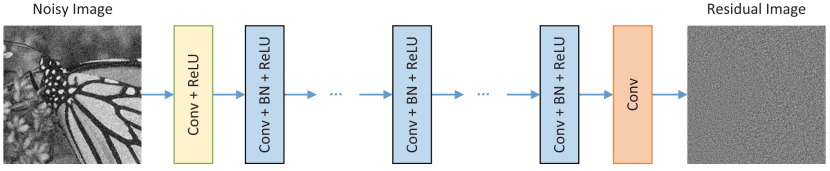
Algorithm A.2 summarizes the PnP-ADMM algorithm for phase retrieval. In this work, we trained the denoiser using the network DnCNN [101]. As shown in Fig. A.2, the architecture of DnCNN consists of convolution (Conv), Rectified Linear Unit (ReLU), and batch normalization(BN). The network was trained with residual learning where the output is the noise residual and the clean image was obtained by subtracting the noisy output. We trained all denoisers for 400 epochs with image patches of size on each given dataset.
Return .
PnP-PGM. Similar to PnP-ADMM, one can also derive a proximal gradient method as shown in Algorithm A.3. Here we assume the denoising of is a proximal operation.
Return .
SD-RED. Regularization by denoising (RED) is an alternative to PnP methods that is based on an explicit image-adaptive regularization functional: . This regularizer reflects the cross-correlation between the image and its denoising residual [51].
Algorithm A.4 summarizes the RED approach for phase retrieval.
Return .
SD-RED-SELF. Other than supervised denoising approaches, we also implemented a self-supervised denoising method known as “noise2self" [53], which designed a neural network to be -invariant so that the self-supervised loss can be represented as the sum of supervised loss and the variance of noise. The “SD-RED-SELF" algorithm refers to training in Algorithm A.4 in such self-supervised fashion on each test data.
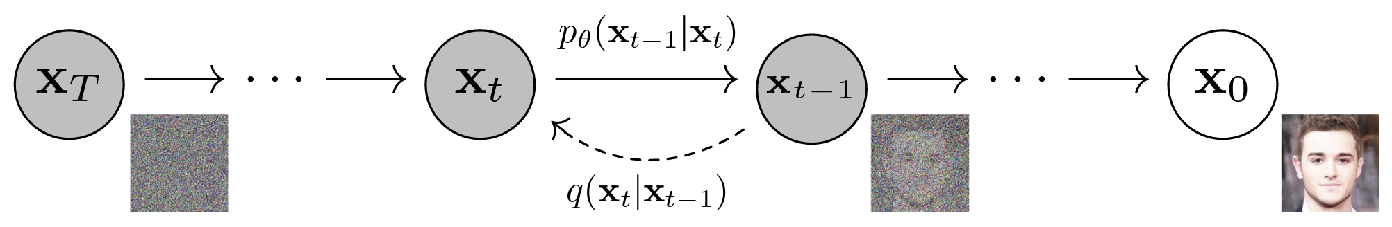
DOLPH. DOLPH is based on the DDPM model [58], which first gradually adds Gaussian noise to data according to a variance schedule so that , as illustrated in Fig. A.3. Using the notation and , we have
| (A.8) |
It can be shown [58] that the appropriate loss function to use is
| (A.9) |
where is selected from . The sampling and reconstruction algorithm requires the addition of noise each step as shown in the following algorithm. Experimentally, however, we found that setting results in higher quality reconstructed images. Furthermore, we choose , , and . For the theory to hold, should be indistinguishable from white Gaussian noise, which is readily verified to be true for these parameters. Finally, the stepsize of the gradient descent step can be chosen according to the Lipschitz constant of the Poisson-Gaussian likelihood to ensure convergence, or empirically, as is done in the experiments.
Acknowledgement
The authors appreciate thoughtful discussions with Arian Eamaz and Farhang Yeganegi from the University of Illinois Chicago (UIC).