Global constraints on non-standard neutrino interactions with quarks and electrons

Abstract

We derive new constraints on effective four-fermion neutrino non-standard interactions with both quarks and electrons. This is done through the global analysis of neutrino oscillation data and measurements of coherent elastic neutrino-nucleus scattering (CE$\nu$NS) obtained with different nuclei. In doing so, we include not only the effects of new physics on neutrino propagation but also on the detection cross section in neutrino experiments which are sensitive to the new physics. We consider both vector and axial-vector neutral-current neutrino interactions and, for each case, we include simultaneously all allowed effective operators in flavour space. To this end, we use the most general parametrization for their Wilson coefficients under the assumption that their neutrino flavour structure is independent of the charged fermion participating in the interaction. The status of the LMA-D solution is assessed for the first time in the case of new interactions taking place simultaneously with up quarks, down quarks, and electrons. One of the main results of our work are the presently allowed regions for the effective combinations of non-standard neutrino couplings, relevant for long-baseline and atmospheric neutrino oscillation experiments.

1 Introduction

The minimal global description of the bulk of data gathered in experiments detecting the interactions of solar and atmospheric neutrinos, and of neutrinos produced in nuclear reactors and in particle accelerators, requires three neutrino states with distinct masses which are non-trivial admixtures of the three flavour neutrino states of the Standard Model (SM). This implies that lepton flavour oscillates with a wavelength which depends on distance and energy Pontecorvo:1967fh ; Gribov:1968kq as required to explain the data, see Ref. GonzalezGarcia:2007ib for an overview. This is one of the most direct indications of physics beyond the Standard Model (BSM).

Given the excellent ability of the SM in explaining the interactions of fundamental particles through the electromagnetic, weak, and strong interactions, it is reasonable to assume that the SM is an effective theory and that new physics (NP) effects are suppressed at low energies. Generic BSM physics can then be introduced in a model-independent manner through a tower of effective operators, suppressed by the heavy NP scale. Interestingly enough, neutrino masses arise in this framework from the unique dimension-five operator consistent with the SM gauge symmetry and particle contents, and therefore can be argued to be the first signal of BSM physics. At next order in the operator expansion we find dimension-six four-fermion operators. Those involving neutrino fields would affect the production, propagation, and detection of neutrinos – the so-called Non-Standard neutrino Interactions (NSI). In this work we focus on operators leading to purely vector or axial-vector interactions (for recent works including additional operators with different Lorentz structures see for example Refs. Falkowski:2021bkq ; Breso-Pla:2023tnz ; Falkowski:2019kfn ; Falkowski:2019xoe ). Generically these can be classified in charged-current (CC) NSI

$$\mathcal{L}_{\text{NSI,CC}}=-2\sqrt{2}\,G_{F}\sum_{f,f^{\prime},\alpha,\beta}\varepsilon_{\alpha\beta}^{ff^{\prime},P}(\bar{\ell}_{\alpha}\gamma_{\mu}P_{L}\nu_{\beta})(\bar{f}\gamma^{\mu}Pf^{\prime})+\text{h.c.}$$ (1)

and neutral-current (NC) NSI

$$\mathcal{L}_{\text{NSI,NC}}=-2\sqrt{2}\,G_{F}\sum_{f,P,\alpha,\beta}\varepsilon_{\alpha\beta}^{f,P}(\bar{\nu}_{\alpha}\gamma^{\mu}P_{L}\nu_{\beta})(\bar{f}\gamma_{\mu}Pf)\,.$$ (2)

In Eqs. (1) and (2), $f$ and $f^{\prime}$ refer to SM charged fermions, $\ell$ denotes a SM charged lepton and $P$ can be either a left-handed or a right-handed projection operator ($P_{L}$ or $P_{R}$, respectively). Moreover the normalization of the couplings is deliberately chosen to match that of the weak currents in the SM, so the values of $\varepsilon_{\alpha\beta}^{f,P}$ indicate the strength of the new interaction with respect to the Fermi constant, $G_{F}$. The corresponding vector and axial-vector combinations of NSI coefficients are defined as:

$$\varepsilon_{\alpha\beta}^{f,V}\equiv\varepsilon_{\alpha\beta}^{f,L}+\varepsilon_{\alpha\beta}^{f,R}\quad\text{and}\quad\varepsilon_{\alpha\beta}^{f,A}\equiv\varepsilon_{\alpha\beta}^{f,L}-\varepsilon_{\alpha\beta}^{f,R}\,.$$ (3)

Precise measurements of meson and muon decays place severe constraints on the possible strength of CC NSI (see for example Refs. Davidson:2003ha ; Biggio:2009nt ; Biggio:2009kv ; Falkowski:2021bkq ). Conversely, NC NSI are much more difficult to probe directly, given the intrinsic difficulties associated to neutrino detection via neutral currents. A priori, the requirement of gauge invariance would generate similar operators in the charged lepton sector, in severe conflict with experimental observables Gavela:2008ra ; Antusch:2008tz . However, such bounds may be alleviated (or evaded) in NP models in which NC NSI are generated by exchange of neutral mediators with masses well below the EW scale (for a recent review on viable NSI models see, e.g., Ref. Dev:2019anc ). It is in these scenarios that one can envision observable effects in present and future neutrino experiments. Several models have been proposed, involving new gauge symmetries and light degrees of freedom, that would give rise to relatively large NC NSI. These include, for example, models where the NSI are generated from the $Z^{\prime}$ boson associated to a new $U(1)^{\prime}$ symmetry Babu:2017olk ; Farzan:2015doa ; Farzan:2016wym ; Farzan:2015hkd ; Greljo:2022dwn ; Heeck:2018nzc ; Farzan:2019xor ; Bernal:2022qba , radiative neutrino mass models involving new scalars Babu:2019mfe , or models with leptoquarks Wise:2014oea ; Greljo:2021npi ; Babu:2019mfe . Many of these extensions involve a gauge symmetry based on a combination of baryon and lepton quantum numbers, and would therefore induce equal NSI for up and down quarks. However, exceptions to this rule arise, for example, in models with leptoquarks where NSI may be only generated for down-quarks Wise:2014oea ; Babu:2019mfe . Similarly it should be stressed that, while many of these models typically lead to diagonal NSI in lepton flavor space, this is not always the case and, depending on the particular extension, sizable off-diagonal NSI may also be obtained (see, e.g., Refs. Farzan:2015hkd ; Farzan:2019xor ; Farzan:2016wym ). In order to derive constraints to such a wide landscape of models, the use of the effective operator approach advocated above is extremely useful. For bounds from oscillation data on $U(1)^{\prime}$ models with diagonal couplings in flavor space, see Ref. Coloma:2020gfv .

In fact, some of the best model-independent bounds on NC NSI are obtained from global fits to oscillation data. These are affected by vector couplings involving fermions present in matter, $\varepsilon_{\alpha\beta}^{f,V}$ with $f\in\{u,d,e\}$, since they modify the effective matter potential Wolfenstein:1977ue ; Mikheev:1986gs felt by neutrinos as they propagate in a medium. In Ref. Gonzalez-Garcia:2013usa such global analysis was performed in the context of vector NC NSI with either up or down quarks. In Ref. Esteban:2018ppq the study was extended to account for the possibility vector NC NSI with up and down quarks simultaneously, under the restriction that the neutrino flavour structure of the NSI interactions is independent of the quark type. However, NSI with electrons were not considered.

One important effect of the presence of NSI Wolfenstein:1977ue ; Valle:1987gv ; Guzzo:1991hi affecting the neutrino propagation in oscillation experiments is the appearance of a degeneracy leading to a qualitative change of the lepton mixing pattern. This was first observed in the context of solar neutrinos, for which the established standard Mikheev-Smirnov-Wolfenstein (MSW) solution Wolfenstein:1977ue ; Mikheev:1986gs requires a mixing angle $\theta_{12}$ in the first octant, while with suitable NSI the data could be described by a mixing angle $\theta_{12}$ in the second octant, the so-called LMA-Dark (LMA-D) Miranda:2004nb solution. The origin of the LMA-D solution is a degeneracy in the oscillation probabilities due to a symmetry of the Hamiltonian describing neutrino evolution in the presence of NSI GonzalezGarcia:2011my ; Gonzalez-Garcia:2013usa ; Bakhti:2014pva ; Coloma:2016gei . Such degeneracy makes it impossible to determine the neutrino mass ordering by oscillation experiments alone Coloma:2016gei and therefore jeopardizes one of the main goals of the upcoming neutrino oscillation program. Although the degeneracy is not exact when including oscillation data from neutrino propagating in different environments, quantitatively the breaking is small and global fits show that the LMA-D solution is still pretty much allowed by oscillation data alone Gonzalez-Garcia:2013usa ; Esteban:2018ppq . A second important limitation of oscillation data is that it is only sensitive to differences in the potential felt by different neutrino flavours. Thus, oscillation data may be used to derive constraints on the differences between diagonal NC NSI parameters, but not on the individual parameters themselves.

Neutrino scattering data is also sensitive to NC NSI as they would affect the interaction rates directly Davidson:2003ha ; Scholberg:2005qs ; Barranco:2005ps ; Barranco:2005yy ; Barranco:2007ej ; Bolanos:2008km . Therefore the combination of oscillation and scattering data may be used to break the LMA-D degeneracy (see for example Refs. Miranda:2004nb ; Escrihuela:2009up for early works on this topic). However, such a combination is most effective whenever the scattering cross section also falls in the contact-interaction regime, since otherwise bounds obtained from scattering may be evaded for sufficiently light mediators Farzan:2015doa . As a consequence, for NSI with quarks the most powerful constraints come from measurements of Coherent Elastic Neutrino-Nucleus Scattering Freedman:1973yd (CE$\nu$NS), since the momentum transfer is small and therefore apply to a wider class of models, as discussed in Refs. Coloma:2016gei ; Coloma:2017egw ; Shoemaker:2017lzs . Reference Coloma:2017ncl showed the impact obtained from the joint analysis of CE$\nu$NS and oscillation data, considering NSI with only one quark type at a time and using the first measurement of CE$\nu$NS at COHERENT COHERENT:2017ipa . Our later works Esteban:2018ppq ; Coloma:2019mbs subsequently improved over this first analysis by including the latest oscillation data, refining the treatment of COHERENT data COHERENT:2018imc and, most importantly, by allowing for NC NSI with up and down quarks simultaneously in the fit, which made the results more general. Moreover, besides lifting the degeneracy, the addition of oscillation and scattering data also allows to obtain separate constraints on the diagonal NSI parameters Coloma:2017ncl .

The field of CE$\nu$NS is moving fast. Since the first measurements on CsI, the COHERENT collaboration has reported a separate measurement using an Ar detector COHERENT:2020iec and the Dresden-II experiment recently reported a signal using a Ge detector Colaresi:2021kus . The combination of CE$\nu$NS measurements for different target nuclei is highly relevant to lift the LMA-D degeneracy for NC NSI with arbitrary couplings to up and down quarks Scholberg:2005qs ; Barranco:2005yy ; Coloma:2017egw ; Chaves:2021pey . Additionally, the combination of data obtained using neutrinos from spallation sources and from reactors may be used to lift degeneracies in NSI flavour space Coloma:2022avw . Therefore, a significant improvement on the bounds for NC NSI with quarks may be expected from the addition of the new datasets that have become recently available.

As mentioned above, the global analyses in Refs. Gonzalez-Garcia:2013usa ; Coloma:2017ncl ; Esteban:2018ppq ; Coloma:2019mbs only included NSI with quarks. However, there is no reason to avoid the new current to couple to electrons as well. The presence of NSI with electrons would affect not only neutrino propagation but also the interaction cross-section for electron scattering (ES). This would impact the data at both SK and Borexino, and makes the problem much more demanding from the computational point of view. Constraints on NC NSI with electrons were obtained from the analysis of Borexino Phase-II spectrum by the Borexino Collaboration Borexino:2019mhy assuming only one NC NSI coupling at a time. Recently, in Ref. Coloma:2022umy we performed an analysis of the Borexino Phase-II spectral data including all NC NSI operators involving electrons simultaneously in the fit. Our results showed that the simultaneous presence of several operators significantly deteriorates the resulting bounds. However, the sensitivity of Borexino to NC NSI with electrons stems mainly from their impact on the detection cross section and not from oscillations. Therefore a significant improvement on the final constraints would be expected from the combination with oscillation data from other experiments. While partial analyses for electron NSI using a subset of data have been performed before Miranda:2004nb ; Escrihuela:2009up ; Bolanos:2008km , an analysis using all available neutrino oscillation data has not been performed yet in this context. Furthermore, the presence of the LMA-D solution in presence of NSI with electrons remains an open question.

In this work we address these open issues by updating and extending our analyses in Refs. Esteban:2018ppq ; Coloma:2019mbs accounting for the possibility of NC NSI with up quarks, down quarks and electrons simultaneously. We will consider vector and axial-vector couplings separately. Our global analysis updates that of our previous works, with the major addition of the Borexino Phase-II spectral dataset. Furthermore when combining with CE$\nu$NS we include the results from COHERENT data on CsI COHERENT:2017ipa ; COHERENT:2018imc and Ar targets COHERENT:2020iec ; COHERENT:2020ybo together with the recent results from CE$\nu$NS searches using reactor neutrinos at Dresden-II reactor experiment Colaresi:2022obx ; Coloma:2022avw . To this aim, in Sec. 2 we briefly summarize the framework of our study. We present the main ingredients and assumptions in the analysis of the NSI effects in the matter potential in atmospheric and long-baseline (LBL) experiments in Sec. 2.1.1, and Solar and KamLAND in Sec. 2.1.2. In particular, we include a discussion on the possible departures from adiabaticity of the evolution of solar neutrinos in Sec. 2.1.3. The effects of NC NSI on the detection cross sections and its interplay with flavour transitions in propagation is reviewed in Sec. 2.2 including the specific modification of the cross section for ES (Sec. 2.2.1), NC scattering with quarks (Sec. 2.2.2), and CE$\nu$NS (Sec. 2.2.3). The results of the different analyses performed are presented in Sec. 3 where we derive our current knowledge of the size and flavour structure of vector NC NSI coupling to either electrons (Sec. 3.2), up and down quarks (Sec. 3.3), or a general combination of those (Sec. 3.4). We study the status of the LMA-D solution as function of the relative strength of the non-standard couplings to the different charged fermions in Sec. 3.5. We also quantify the results as allowed ranges of the effective combinations of couplings relevant for long-baseline and atmospheric oscillation experiments. In Sec. 4 we summarize our conclusions.

2 Formalism

As stated in the introduction, in this work we will consider NC NSI (hereafter referred to simply as NSI, for brevity) relevant to neutrino scattering and propagation in matter, as parametrized in Eq. (2). To make the analysis feasible, the following simplifications are introduced:

• we assume that the neutrino flavour structure of the interactions is independent of the charged fermion properties;

• we further assume that the chiral structure of the charged fermion vertex is the same for all fermion types.

Under these hypotheses, we can factorize $\varepsilon_{\alpha\beta}^{f,P}$ as the product of three terms:

$$\varepsilon_{\alpha\beta}^{f,P}\equiv\varepsilon_{\alpha\beta}\,\xi^{f}\chi^{P}$$ (4)

where the matrix $\varepsilon_{\alpha\beta}$ describes the dependence on the neutrino flavour, the coefficients $\xi^{f}$ parametrize the coupling to the charged fermions, and the terms $\chi^{P}$ account for the chiral structure of such couplings, normalized so that $\varepsilon_{\alpha\beta}^{f,L}$ ($\varepsilon_{\alpha\beta}^{f,R}$) corresponds to $\chi^{L}=1/2$ and $\chi^{R}=0$ ($\chi^{R}=1/2$ and $\chi^{L}=0$). With these assumptions the Lagrangian in Eq. (2) takes the form:

$$\mathcal{L}_{\text{NSI,NC}}=-2\sqrt{2}G_{F}\bigg{[}\sum_{\alpha,\beta}\varepsilon_{\alpha\beta}(\bar{\nu}_{\alpha}\gamma^{\mu}P_{L}\nu_{\beta})\bigg{]}\bigg{[}\sum_{f,P}\xi^{f}\chi^{P}(\bar{f}\gamma_{\mu}Pf)\bigg{]}\,.$$ (5)

Concerning the chiral structure of the charged fermion vertex, in this work we will consider either vector couplings ($\chi^{L}=\chi^{R}=1/2$), or axial-vector couplings ($\chi^{L}=-\chi^{R}=1/2)$. The corresponding combinations of NSI coefficients are given in Eq. (3).

For what concerns the dependence of the NSI on the charged fermion type, we notice that ordinary matter is composed of electrons ($e$), up quarks ($u$) and down quarks ($d$), so that only the coefficients $\xi^{e}$, $\xi^{u}$ and $\xi^{d}$ are experimentally accessible. For vector NSI, since quarks are always confined inside protons ($p$) and neutrons ($n$), we may define (see, e.g., Ref. Breso-Pla:2023tnz ):

$$\xi^{p}=2\xi^{u}+\xi^{d}\,,\qquad\xi^{n}=2\xi^{d}+\xi^{u}$$ (6)

so that $\varepsilon_{\alpha\beta}^{p,V}\equiv 2\varepsilon_{\alpha\beta}^{u,V}+\varepsilon_{\alpha\beta}^{d,V}=\varepsilon_{\alpha\beta}\,\xi^{p}\,(\chi^{L}+\chi^{R})$ and $\varepsilon_{\alpha\beta}^{n,V}\equiv 2\varepsilon_{\alpha\beta}^{d,V}+\varepsilon_{\alpha\beta}^{u,V}=\varepsilon_{\alpha\beta}\,\xi^{n}\,(\chi^{L}+\chi^{R})$. For axial-vector NSI, the correspondence between quark NSI and nucleon NSI is not that obvious: for example, for non-relativistic nucleons an axial-vector hadronic current would induce a change in the spin of the nucleon. In our analysis this type of NSI is only relevant for the breakup of deuterium at SNO as discussed in Sec. 2.2.2. In any case, it is clear that a simultaneous re-scaling of all $\{\xi^{f}\}$ by a common factor can be reabsorbed into a re-scaling of $\varepsilon_{\alpha\beta}$, so that only the direction of $(\xi^{e},\xi^{u},\xi^{d})$ – or, equivalently, $(\xi^{e},\xi^{p},\xi^{n})$ – is phenomenologically non-trivial. We parametrize such direction using spherical coordinates, in terms of a “latitude” angle $\eta$ and a “longitude” angle $\zeta$, as an extension of the framework and notation introduced in Ref. Esteban:2018ppq (see also Ref. Amaral:2023tbs ). Concretely, we define:

$$\xi^{e}=\sqrt{5}\cos\eta\sin\zeta\,,\qquad\xi^{p}=\sqrt{5}\cos\eta\cos\zeta\,,\qquad\xi^{n}=\sqrt{5}\sin\eta$$ (7)

or, in terms of the “quark” couplings:

$$\xi^{u}=\frac{\sqrt{5}}{3}(2\cos\eta\cos\zeta-\sin\eta)\,,\qquad\xi^{d}=\frac{\sqrt{5}}{3}(2\sin\eta-\cos\eta\cos\zeta)$$ (8)

Using this parametrization, the case of NSI with quarks analyzed in Ref. Esteban:2018ppq correspond to the “prime meridian” $\zeta=0$, with the pure up-quark and pure down-quark cases located at $\eta=\arctan(1/2)\approx 26.6^{\circ}$ and $\eta=\arctan(2)\approx 63.4^{\circ}$, respectively. The “poles” ($\eta=\pm 90^{\circ}$) correspond to NSI with neutrons, while NSI with protons lies on the “equator” ($\eta=\zeta=0$). Finally, the pure electron case is also on the equator, at a right angle ($\zeta=\pm 90^{\circ}$) from the pure proton case. Notice that an overall sign flip of $(\xi^{e},\xi^{u},\xi^{d})$ is just a special case of re-scaling and produces no observable effect, hence it is sufficient to restrict both $\eta$ and $\zeta$ to the $[-90^{\circ},+90^{\circ}]$ range.

The presence of vector NC NSI will affect both neutrino propagation in matter and neutrino scattering in the detector, while axial-vector NC NSI only affect some of the interaction cross sections. Both propagation and interaction effects lead to a modification of the expected number of events which can be described by the generic expression Coloma:2022umy :

$$N_{\text{ev}}\propto\operatorname{Tr}\Big{[}\rho^{\text{det}}\,\sigma^{\text{det}}\Big{]}$$ (9)

where $\rho^{\text{det}}$ is the density matrix characterizing the flavour state of the neutrinos reaching the detector, while the generalized cross section $\sigma^{\text{det}}$ is a matrix in flavour space containing enough information to describe the interaction of any neutrino configuration. The form of Eq. (9) is manifestly basis-independent and permits a separate description of propagation effects (encoded into $\rho^{\text{det}}$) and of the scattering process (contained in $\sigma^{\text{det}}$), while at the same time properly taking into account possible interference between them. Notice that both $\rho^{\text{det}}$ and $\sigma^{\text{det}}$ are hermitian matrices, which ensures that $N_{\text{ev}}$ is real. Actually, Eq. (9) is invariant under the joint transformation:

$$\rho^{\text{det}}\to\big{[}\rho^{\text{det}}\big{]}^{*}\quad\text{and}\quad\sigma^{\text{det}}\to\big{[}\sigma^{\text{det}}\big{]}^{*}$$ (10)

whose implications will be discussed later on in this section.

2.1 Neutrino oscillations in the presence of NSI

In general, the evolution of the neutrino and antineutrino flavour state during propagation is governed by the Hamiltonian:

$$H^{\nu}=H_{\text{vac}}+H_{\text{mat}}\quad\text{and}\quad H^{\bar{\nu}}=(H_{\text{vac}}-H_{\text{mat}})^{*}\,,$$ (11)

where $H_{\text{vac}}$ is the vacuum part which in the flavour basis $(\nu_{e},\nu_{\mu},\nu_{\tau})$ reads

$$H_{\text{vac}}=U_{\text{vac}}D_{\text{vac}}U_{\text{vac}}^{\dagger}\quad\text{with}\quad D_{\text{vac}}=\frac{1}{2E_{\nu}}\operatorname{diag}(0,\Delta m^{2}_{21},\Delta m^{2}_{31})\,.$$ (12)

Here $U_{\text{vac}}$ denotes the three-lepton mixing matrix in vacuum Pontecorvo:1967fh ; Maki:1962mu ; Kobayashi:1973fv . Following the convention of Ref. Coloma:2016gei , we define $U_{\text{vac}}=R_{23}(\theta_{23})R_{13}(\theta_{13})\tilde{R}_{12}(\theta_{12},\delta_{\text{CP}})$, where $R_{ij}(\theta_{ij})$ is a rotation of angle $\theta_{ij}$ in the $ij$ plane and $\tilde{R}_{12}(\theta_{12},\delta_{\text{CP}})$ is a complex rotation by angle $\theta_{12}$ and phase $\delta_{\text{CP}}$. Explicitly:

$$U_{\text{vac}}=\begin{pmatrix}c_{12}c_{13}&s_{12}c_{13}e^{i\delta_{\text{CP}}}&s_{13}\\ -s_{12}c_{23}e^{-i\delta_{\text{CP}}}-c_{12}s_{13}s_{23}&\hphantom{+}c_{12}c_{23}-s_{12}s_{13}s_{23}e^{i\delta_{\text{CP}}}&c_{13}s_{23}\\ \hphantom{+}s_{12}s_{23}e^{-i\delta_{\text{CP}}}-c_{12}s_{13}c_{23}&-c_{12}s_{23}-s_{12}s_{13}c_{23}e^{i\delta_{\text{CP}}}&c_{13}c_{23}\end{pmatrix}$$ (13)

where $c_{ij}\equiv\cos\theta_{ij}$ and $s_{ij}\equiv\sin\theta_{ij}$. This expression differs from the usual one “$U$” (defined, e.g., in Eq. (1.1) of Ref. Esteban:2016qun ) by an overall phase matrix: $U_{\text{vac}}=PUP^{*}$ with $P=\operatorname{diag}(e^{i\delta_{\text{CP}}},1,1)$. It is easy to show that, in the absence of NSI, such rephasing produces no visible effect, so that when only standard interactions are considered the physical interpretation of the vacuum parameters ($\Delta m^{2}_{21}$, $\Delta m^{2}_{31}$, $\theta_{12}$, $\theta_{13}$, $\theta_{23}$ and $\delta_{\text{CP}}$) is exactly the same in both conventions. The advantage of defining $U_{\text{vac}}$ as in Eq. (13) is that the transformation $H_{\text{vac}}\to-H_{\text{vac}}^{*}$, whose relevance for the present work will be discussed below, can be implemented exactly (up to an irrelevant multiple of the identity) by the following transformation of the parameters:

$$\Delta m^{2}_{31} \to-\Delta m^{2}_{31}+\Delta m^{2}_{21}=-\Delta m^{2}_{32}\,,$$ (14)

$$\theta_{12} \to\pi/2-\theta_{12}\,,$$

$$\delta_{\text{CP}} \to\pi-\delta_{\text{CP}}$$

which does not spoil the commonly assumed restrictions on the range of the vacuum parameters ($\Delta m^{2}_{21}>0$ and $0\leq\theta_{ij}\leq\pi/2$).

Concerning the matter part $H_{\text{mat}}$ of the Hamiltonian which governs neutrino oscillations, if all possible operators in Eq. (2) are added to the SM Lagrangian we get:

$$H_{\text{mat}}=\sqrt{2}G_{F}N_{e}(x)\begin{pmatrix}1+\mathcal{E}_{ee}(x)&\mathcal{E}_{e\mu}(x)&\mathcal{E}_{e\tau}(x)\\ \mathcal{E}_{e\mu}^{*}(x)&\mathcal{E}_{\mu\mu}(x)&\mathcal{E}_{\mu\tau}(x)\\ \mathcal{E}_{e\tau}^{*}(x)&\mathcal{E}_{\mu\tau}^{*}(x)&\mathcal{E}_{\tau\tau}(x)\end{pmatrix}$$ (15)

where the “$+1$” term in the $ee$ entry accounts for the standard contribution, and

$$\mathcal{E}_{\alpha\beta}(x)=\sum_{f=e,u,d}\frac{N_{f}(x)}{N_{e}(x)}\varepsilon_{\alpha\beta}^{f,V}$$ (16)

describes the non-standard part. Here $N_{f}(x)$ is the number density of fermion $f$ as a function of the distance traveled by the neutrino along its trajectory. In Eq. (16) we have limited the sum to the charged fermions present in ordinary matter, $f=e,u,d$. Taking into account that $N_{u}(x)=2N_{p}(x)+N_{n}(x)$ and $N_{d}(x)=N_{p}(x)+2N_{n}(x)$, and also that matter neutrality implies $N_{p}(x)=N_{e}(x)$, Eq. (16) becomes:

$$\mathcal{E}_{\alpha\beta}(x)=\big{(}\varepsilon_{\alpha\beta}^{e,V}+\varepsilon_{\alpha\beta}^{p,V}\big{)}+Y_{n}(x)\,\varepsilon_{\alpha\beta}^{n,V}\quad\text{with}\quad Y_{n}(x)\equiv\frac{N_{n}(x)}{N_{e}(x)}$$ (17)

which shows that, from the phenomenological point of view, the propagation effects of NSI with electrons can be mimicked by NSI with quarks by means of a suitable combination of up-quark and down-quark contributions.

Since the matter potential can be determined by oscillation experiments only up to an overall multiple of the identity, each $\varepsilon_{\alpha\beta}^{f,V}$ matrix introduces 8 new parameters: two differences of the three diagonal real parameters (e.g., $\varepsilon_{ee}^{f,V}-\varepsilon_{\mu\mu}^{f,V}$ and $\varepsilon_{\tau\tau}^{f,V}-\varepsilon_{\mu\mu}^{f,V}$) and three off-diagonal complex parameters (i.e., three additional moduli and three complex phases). Under the assumption that the neutrino flavour structure of the interactions is independent of the charged fermion type, as described in Eq. (4), we get:

$$\mathcal{E}_{\alpha\beta}(x) =\varepsilon_{\alpha\beta}\big{[}\xi^{e}+\xi^{p}+Y_{n}(x)\xi^{n}\big{]}\big{(}\chi^{L}+\chi^{R}\big{)}$$ (18)

$$=\sqrt{5}\,\big{[}\!\cos\eta\,(\cos\zeta+\sin\zeta)+Y_{n}(x)\sin\eta\big{]}\big{(}\chi^{L}+\chi^{R}\big{)}\,\varepsilon_{\alpha\beta}$$

so that the phenomenological framework adopted here is characterized by 10 matter parameters: eight related to the matrix $\varepsilon_{\alpha\beta}$ plus two directions $(\eta,\zeta)$ in the $(\xi^{e},\xi^{p},\xi^{n})$ space. Notice, however, that the dependence on $\zeta$ in Eq. (18) can be reabsorbed into a re-scaling of $\varepsilon_{\alpha\beta}$ by introducing a new effective angle $\eta^{\prime}$:

$$\mathcal{E}_{\alpha\beta}(x)=\sqrt{5}\,\big{[}\!\cos\eta^{\prime}+Y_{n}(x)\sin\eta^{\prime}\big{]}\big{(}\chi^{L}+\chi^{R}\big{)}\,\varepsilon_{\alpha\beta}^{\prime}\\ \text{with}\quad\tan\eta^{\prime}\equiv\tan\eta\mathbin{\big{/}}(\cos\zeta+\sin\zeta)\quad\text{and}\quad\varepsilon_{\alpha\beta}^{\prime}\equiv\varepsilon_{\alpha\beta}\sqrt{1+\cos^{2}\eta\sin(2\zeta)}\,.$$ (19)

This is a consequence of the fact that electron and proton NSI always appear together in propagation, as explained after Eq. (17). Indeed, $\eta^{\prime}$ is just a practical way to express the direction in the $(\xi^{e}+\xi^{p},\,\xi^{n})$ plane. For $\zeta=0$, which is the case studied in Ref. Esteban:2018ppq , one trivially recovers $\eta^{\prime}=\eta$ and $\varepsilon_{\alpha\beta}^{\prime}=\varepsilon_{\alpha\beta}$. Furthermore, for $\zeta=-45^{\circ}$ one gets $\xi^{e}+\xi^{p}=0$, so that NSI effects in oscillations depend solely on the neutron coupling $\xi^{n}$. This would be the case, for example, in models where the $Z^{\prime}$ does not couple directly to matter fermions, and NSI are generated through $Z-Z^{\prime}$ mass mixing (see the related discussion in Ref. Heeck:2018nzc ). In fact, in this case, the specific value of $\eta$ becomes irrelevant as long as it is different from zero (since Eq. (19) always yields $\eta^{\prime}=\pm 90^{\circ}$ in this case), while for the special point where $\eta=0$ and $\zeta=-45^{\circ}$ NSI completely cancel from oscillations. It should be stressed, however, that this only applies to oscillations: the implications of NSI for neutrino scattering described in Sec. 2.2 will still depend non-trivially on $\eta$.

We finish this section by reminding that the neutrino transition probabilities remain invariant – and more generically the density matrix $\rho^{\text{det}}$ undergoes complex conjugation, as described in Eq. (10) – if the Hamiltonian $H^{\nu}=H_{\text{vac}}+H_{\text{mat}}$ is transformed as $H^{\nu}\to-(H^{\nu})^{*}$. This requires a simultaneous transformation of both the vacuum and the matter terms. The transformation of $H_{\text{vac}}$ is described in Eq. (14) and involves a change in the octant of $\theta_{12}$ (the so-called LMA-D Miranda:2004nb solution) as well as a change in the neutrino mass ordering (i.e., the sign of $\Delta m^{2}_{31}$), which is why it has been called “generalized mass-ordering degeneracy” in Ref. Coloma:2016gei . As for $H_{\text{mat}}$ we need:

$$\big{[}\mathcal{E}_{ee}(x)-\mathcal{E}_{\mu\mu}(x)\big{]} \to-\big{[}\mathcal{E}_{ee}(x)-\mathcal{E}_{\mu\mu}(x)\big{]}-2\,,$$ (20)

$$\big{[}\mathcal{E}_{\tau\tau}(x)-\mathcal{E}_{\mu\mu}(x)\big{]} \to-\big{[}\mathcal{E}_{\tau\tau}(x)-\mathcal{E}_{\mu\mu}(x)\big{]}\,,$$

$$\mathcal{E}_{\alpha\beta}(x) \to-\mathcal{E}_{\alpha\beta}^{*}(x)\qquad(\alpha\neq\beta)\,,$$

see Refs. Gonzalez-Garcia:2013usa ; Bakhti:2014pva ; Coloma:2016gei . As seen in Eqs. (16), (17) and (18) the matrix $\mathcal{E}_{\alpha\beta}(x)$ depends on the chemical composition of the medium, which may vary along the neutrino trajectory, so that in general the condition in Eq. (20) is fulfilled only in an approximate way. The degeneracy becomes exact in the following two cases:

• if the effective NSI coupling to neutrons vanishes, so that $\varepsilon_{\alpha\beta}^{n,V}=0$ in Eq. (17). In terms of fundamental quantities this occurs when $\varepsilon_{\alpha\beta}^{u,V}=-2\varepsilon_{\alpha\beta}^{d,V}$, i.e., the NSI couplings are proportional to the electric charge of quarks. In our parametrization this corresponds to the “equator” $\eta=0$ for arbitrary $\zeta$, as shown in Eq. (18);

• if the neutron/proton ratio $Y_{n}(x)$ is constant along the entire neutrino propagation path. This is certainly the case for reactor and long-baseline experiments, where only the Earth’s mantle is involved, and to a good approximation also for atmospheric neutrinos, since the differences in chemical composition between mantle and core can safely be neglected in the context of NSI GonzalezGarcia:2011my . In this case the matrix $\mathcal{E}_{\alpha\beta}(x)$ becomes independent of $x$ and can be regarded as a new phenomenological parameter, as we will describe in Sec. 2.1.1.

Further details on the implications of this degeneracy for different classes of neutrino experiments (solar, atmospheric, etc.) is provided below in the corresponding section.

2.1.1 Matter potential in atmospheric and long-baseline neutrinos

As discussed in Ref. GonzalezGarcia:2011my , in the Earth the neutron/proton ratio $Y_{n}(x)$ which characterizes the matter chemical composition can be taken to be constant to very good approximation. The PREM model Dziewonski:1981xy fixes $Y_{n}=1.012$ in the Mantle and $Y_{n}=1.137$ in the Core, with an average value $Y_{n}^{\oplus}=1.051$ all over the Earth. Setting therefore $Y_{n}(x)\equiv Y_{n}^{\oplus}$ in Eqs. (16) and (17) we get $\mathcal{E}_{\alpha\beta}(x)\equiv\varepsilon_{\alpha\beta}^{\oplus}$ with:

$$\varepsilon_{\alpha\beta}^{\oplus}=\varepsilon_{\alpha\beta}^{e,V}+\big{(}2+Y_{n}^{\oplus}\big{)}\varepsilon_{\alpha\beta}^{u,V}+\big{(}1+2Y_{n}^{\oplus}\big{)}\varepsilon_{\alpha\beta}^{d,V}=\big{(}\varepsilon_{\alpha\beta}^{e,V}+\varepsilon_{\alpha\beta}^{p,V}\big{)}+Y_{n}^{\oplus}\varepsilon_{\alpha\beta}^{n,V}\,.$$ (21)

If we impose quark-lepton factorization as in Eq. (18) we get:

$$\varepsilon_{\alpha\beta}^{\oplus} =\sqrt{5}\,\big{[}\!\cos\eta\,(\cos\zeta+\sin\zeta)+Y_{n}^{\oplus}\sin\eta\big{]}\big{(}\chi^{L}+\chi^{R}\big{)}\,\varepsilon_{\alpha\beta}$$ (22)

$$=\sqrt{5}\,\big{[}\!\cos\eta^{\prime}+Y_{n}^{\oplus}\sin\eta^{\prime}\big{]}\big{(}\chi^{L}+\chi^{R}\big{)}\,\varepsilon_{\alpha\beta}^{\prime}\,.$$

In other words, within this approximation the analysis of atmospheric and LBL neutrinos holds for any combination of NSI with up, down or electrons and it can be performed in terms of the effective NSI couplings $\varepsilon_{\alpha\beta}^{\oplus}$, which play the role of phenomenological parameters. In particular, the best-fit value and allowed ranges of $\varepsilon_{\alpha\beta}^{\oplus}$ are independent of $\eta$ and $\zeta$, while the bounds on $\varepsilon_{\alpha\beta}$ simply scale as $[\cos\eta\,(\cos\zeta+\sin\zeta)+Y_{n}^{\oplus}\sin\eta]$. Moreover, it is immediate to see that for $\eta^{\prime}=\arctan(-1/Y_{n}^{\oplus})\approx-43.6^{\circ}$, with $\eta^{\prime}$ defined in Eq. (19), the contribution of NSI to the matter potential vanishes, so that no bound on $\varepsilon_{\alpha\beta}$ can be derived from atmospheric and LBL data in such case. This would be approximately the case, for example, for $U(1)^{\prime}$ models associated to the combination $B-2L_{e}+\alpha L_{\mu}-\beta L_{\tau}$ and, consequently, oscillation bounds are significantly relaxed for this type of models Greljo:2022dwn .

Following the approach of Ref. GonzalezGarcia:2011my , the matter Hamiltonian $H_{\text{mat}}$, given in Eq. (15) after setting $\mathcal{E}_{\alpha\beta}(x)\equiv\varepsilon_{\alpha\beta}^{\oplus}$, can be parametrized in a way that mimics the structure of the vacuum term (12):

$$H_{\text{mat}}=Q_{\text{rel}}U_{\text{mat}}D_{\text{mat}}U_{\text{mat}}^{\dagger}Q_{\text{rel}}^{\dagger}\text{~{}~{}with~{}~{}}\left\{\begin{aligned} Q_{\text{rel}}&=\operatorname{diag}\left(e^{i\alpha_{1}},e^{i\alpha_{2}},e^{-i\alpha_{1}-i\alpha_{2}}\right),\\ U_{\text{mat}}&=R_{12}(\varphi_{12})R_{13}(\varphi_{13})\tilde{R}_{23}(\varphi_{23},\delta_{\text{NS}})\,,\\ D_{\text{mat}}&=\sqrt{2}G_{F}N_{e}(x)\operatorname{diag}(\varepsilon_{\oplus},\varepsilon_{\oplus}^{\prime},0)\end{aligned}\right.$$ (23)

where $R_{ij}(\varphi_{ij})$ is a rotation of angle $\varphi_{ij}$ in the $ij$ plane and $\tilde{R}_{23}(\varphi_{23},\delta_{\text{NS}})$ is a complex rotation by angle $\varphi_{23}$ and phase $\delta_{\text{NS}}$. Note that the two phases $\alpha_{1}$ and $\alpha_{2}$ included in $Q_{\text{rel}}$ are not a feature of neutrino-matter interactions, but rather a relative feature of the vacuum and matter terms. In order to simplify the analysis we impose that two eigenvalues of $H_{\text{mat}}$ are equal, $\varepsilon_{\oplus}^{\prime}=0$. This assumption is justified since, as shown in Ref. Friedland:2004ah , in this case strong cancellations in the oscillation of atmospheric neutrinos occur, and this is precisely the situation in which the weakest constraints can be placed. Setting $\varepsilon_{\oplus}^{\prime}\to 0$ implies that the $\varphi_{23}$ angle and the $\delta_{\text{NS}}$ phase disappear from neutrino oscillations, so that the effective NSI couplings $\varepsilon_{\alpha\beta}^{\oplus}$ can be parametrized as:

$$\varepsilon_{ee}^{\oplus}-\varepsilon_{\mu\mu}^{\oplus} =\hphantom{-}\varepsilon_{\oplus}\,(\cos^{2}\varphi_{12}-\sin^{2}\varphi_{12})\cos^{2}\varphi_{13}-1\,,$$ (24)

$$\varepsilon_{\tau\tau}^{\oplus}-\varepsilon_{\mu\mu}^{\oplus} =\hphantom{-}\varepsilon_{\oplus}\,(\sin^{2}\varphi_{13}-\sin^{2}\varphi_{12}\,\cos^{2}\varphi_{13})\,,$$

$$\varepsilon_{e\mu}^{\oplus} =-\varepsilon_{\oplus}\,\cos\varphi_{12}\,\sin\varphi_{12}\,\cos^{2}\varphi_{13}\,e^{i(\alpha_{1}-\alpha_{2})}\,,$$

$$\varepsilon_{e\tau}^{\oplus} =-\varepsilon_{\oplus}\,\cos\varphi_{12}\,\cos\varphi_{13}\,\sin\varphi_{13}\,e^{i(2\alpha_{1}+\alpha_{2})}\,,$$

$$\varepsilon_{\mu\tau}^{\oplus} =\hphantom{-}\varepsilon_{\oplus}\,\sin\varphi_{12}\,\cos\varphi_{13}\,\sin\varphi_{13}\,e^{i(\alpha_{1}+2\alpha_{2})}\,.$$

As further simplification, in order to keep the fit manageable we assume real NSI, which we implement by choosing $\alpha_{1}=\alpha_{2}=0$ and $-\pi/2\leq\varphi_{ij}\leq\pi/2$, and also restrict $\delta_{\text{CP}}\in\{0,\pi\}$. It is important to note that with these approximations the formalism for atmospheric and long-baseline data is CP-conserving; we will go back to this point when discussing the experimental results included in the fit. In addition to atmospheric and LBL experiments, important information on neutrino oscillation parameters is provided also by reactor experiments with a baseline of about 1 km. Due to the very small amount of matter crossed, both standard and non-standard matter effects are completely irrelevant for these experiments, so that neutrino propagation depends only on the vacuum parameters.

2.1.2 Matter potential for solar and KamLAND neutrinos

For the study of propagation of solar and KamLAND neutrinos one can work in the one mass dominance approximation, $\Delta m^{2}_{31}\to\infty$ (which effectively means that $G_{F}\sum_{f}N_{f}(x)\,\varepsilon_{\alpha\beta}^{f,V}\ll\Delta m^{2}_{31}/E_{\nu}$). In this limit the neutrino evolution can be calculated in an effective $2\times 2$ model described by the Hamiltonian $H_{\text{eff}}=H_{\text{vac}}^{\text{eff}}+H_{\text{mat}}^{\text{eff}}$, with:

$$H_{\text{vac}}^{\text{eff}} =\frac{\Delta m^{2}_{21}}{4E_{\nu}}\begin{pmatrix}-\cos 2\theta_{12}\,\hphantom{e^{-i\delta_{\text{CP}}}}&~{}\sin 2\theta_{12}\,e^{i\delta_{\text{CP}}}\\ \hphantom{-}\sin 2\theta_{12}\,e^{-i\delta_{\text{CP}}}&~{}\cos 2\theta_{12}\,\hphantom{e^{i\delta_{\text{CP}}}}\end{pmatrix},$$ (25)

$$H_{\text{mat}}^{\text{eff}} =\sqrt{2}G_{F}N_{e}(x)\left[\frac{c_{13}^{2}}{2}\begin{pmatrix}1&\hphantom{-}0\\ 0&-1\end{pmatrix}+\big{[}\xi^{e}+\xi^{p}+Y_{n}(x)\xi^{n}\big{]}\big{(}\chi^{L}+\chi^{R}\big{)}\!\begin{pmatrix}-\varepsilon_{D}^{\hphantom{*}}&\varepsilon_{N}\\ \hphantom{+}\varepsilon_{N}^{*}&\varepsilon_{D}\end{pmatrix}\right],$$ (26)

where we have imposed the quark-lepton factorization of Eq. (18) and used the parametrization convention of Eq. (13) for $U_{\text{vac}}$. The coefficients $\varepsilon_{D}$ and $\varepsilon_{N}$ are related to the original parameters $\varepsilon_{\alpha\beta}$ by the following relations:

$$\begin{split}\varepsilon_{D}&=c_{13}s_{13}\,\mathop{\mathrm{Re}}\!\big{(}s_{23}\,\varepsilon_{e\mu}+c_{23}\,\varepsilon_{e\tau}\big{)}-\big{(}1+s_{13}^{2}\big{)}\,c_{23}s_{23}\,\mathop{\mathrm{Re}}\!\big{(}\varepsilon_{\mu\tau}\big{)}\\ &\hphantom{={}}-\frac{c_{13}^{2}}{2}\big{(}\varepsilon_{ee}-\varepsilon_{\mu\mu}\big{)}+\frac{s_{23}^{2}-s_{13}^{2}c_{23}^{2}}{2}\big{(}\varepsilon_{\tau\tau}-\varepsilon_{\mu\mu}\big{)}\,,\end{split}$$ (27)

$$\varepsilon_{N} =c_{13}\big{(}c_{23}\,\varepsilon_{e\mu}-s_{23}\,\varepsilon_{e\tau}\big{)}+s_{13}\left[s_{23}^{2}\,\varepsilon_{\mu\tau}-c_{23}^{2}\,\varepsilon_{\mu\tau}^{*}+c_{23}s_{23}\big{(}\varepsilon_{\tau\tau}-\varepsilon_{\mu\mu}\big{)}\right].$$ (28)

Denoting by $S_{\text{eff}}$ the $2\times 2$ unitary matrix obtained integrating $H_{\text{eff}}$ along the neutrino trajectory, the full density matrix $\rho^{\text{det}}$ introduced in Eq. (9) can be written as:

$$\rho_{\alpha\beta}^{\text{det}}=c_{13}^{2}\big{[}A_{\alpha\beta}P_{\text{osc}}+B_{\alpha\beta}P_{\text{int}}+iC_{\alpha\beta}P_{\text{ext}}\big{]}+D_{\alpha\beta}$$ (29)

where the effective probabilities $P_{\text{osc}}$, $P_{\text{int}}$ and $P_{\text{ext}}$ are given by

$$P_{\text{osc}}\equiv|S_{21}^{\text{eff}}|^{2}\,,\qquad P_{\text{int}}\equiv\mathop{\mathrm{Re}}\big{(}S_{11}^{\text{eff}}S_{21}^{\text{eff}\,*}\big{)}\,,\qquad P_{\text{ext}}\equiv\mathop{\mathrm{Im}}\big{(}S_{11}^{\text{eff}}S_{21}^{\text{eff}\,*}\big{)}\,,$$ (30)

and the numerical coefficients $A_{\alpha\beta}$, $B_{\alpha\beta}$, $C_{\alpha\beta}$ and $D_{\alpha\beta}$ are defined as

$$A_{\alpha\beta} \equiv O_{\alpha 2}O_{\beta 2}-O_{\alpha 1}O_{\beta 1}\,, \qquad B_{\alpha\beta} \equiv O_{\alpha 1}O_{\beta 2}+O_{\alpha 2}O_{\beta 1}\,,$$ (31)

$$C_{\alpha\beta} \equiv O_{\alpha 1}O_{\beta 2}-O_{\alpha 2}O_{\beta 1}\,, \qquad D_{\alpha\beta} \equiv\sum_{i=\text{all}}O_{\alpha i}O_{\beta i}|O_{ei}|^{2}\,.$$

with $O=R_{23}(\theta_{23})R_{13}(\theta_{13})$. Unlike in Ref. Esteban:2018ppq where NSI did not affect the scattering process and only the $\rho_{ee}^{\text{det}}$ entry (which depends exclusively on $P_{\text{osc}}$) was required, a rephasing of $S_{\text{eff}}$ now produces visible consequences as it affects $P_{\text{int}}$ and $P_{\text{ext}}$. Moreover, $\nu_{\mu}$ and $\nu_{\tau}$ are no longer indistinguishable as their scattering amplitude may be different under NSI, so that the $\theta_{23}$ angle acquires relevance. Hence, for each fixed value of $\eta$ and $\zeta$ the density matrix $\rho^{\text{det}}$ for solar and KamLAND neutrinos depends effectively on eight quantities: the four real oscillation parameters $\theta_{12}$, $\theta_{13}$, $\theta_{23}$ and $\Delta m^{2}_{21}$, the real $\varepsilon_{D}$ and complex $\varepsilon_{N}$ matter parameters, and the CP phase $\delta_{\text{CP}}$. As stated in Sec. 2.1.1 in this work we will assume real NSI, implemented here by setting $\delta_{\text{CP}}\in\{0,\pi\}$ and considering only real values for $\varepsilon_{N}$.

Unlike in the Earth, the matter chemical composition of the Sun varies substantially along the neutrino trajectory, and consequently the potential depends non-trivially on the specific combinations of $(\xi^{e}+\xi^{p})$ and $\xi^{n}$ couplings – i.e., on the value of $\eta^{\prime}$ as determined by the $(\eta,\zeta)$ parameters. This implies that the generalized mass-ordering degeneracy is not exact, except for $\eta=0$ (in which case the NSI potential is proportional to the standard MSW potential and an exact inversion of the matter sign is possible). However the transformation described in Eqs. (14) and (20) still results in a good fit to the global analysis of oscillation data for a wide range of values of $\eta^{\prime}$, and non-oscillation data are needed to break this degeneracy Coloma:2016gei .

2.1.3 Departures from adiabaticity in presence of NSI

When computing neutrino evolution in the Sun, it is often assumed that it takes place in the adiabatic regime, as this considerably simplifies the calculation. While this is the case for neutrino oscillations within the LMA solution with a standard matter potential, it is worthwhile asking if the inclusion of NP effects (such as NSI) can lead to non-adiabatic transitions. If this were the case, it would require special care and may lead to interesting new phenomenological consequences. This possibility has been largely overlooked in the literature, where most studies of NSI in the Sun assume adiabatic transitions.

Let us consider the two-neutrino case, with a matter potential that depends on the position $x$ along the neutrino path inside the Sun. In the instantaneous mass basis, the Hamiltonian can be written as:

$$i\frac{\mathrm{d}}{\mathrm{d}x}\begin{pmatrix}\tilde{\nu}_{1}\\ \tilde{\nu}_{2}\end{pmatrix}=\begin{pmatrix}-\Delta_{m}(x)\enspace&-i\theta_{m}^{\prime}(x)\\ i\theta_{m}^{\prime}(x)&\Delta_{m}(x)\end{pmatrix}\begin{pmatrix}\tilde{\nu}_{1}\\ \tilde{\nu}_{2}\end{pmatrix}$$ (32)

where $\theta_{m}(x)$ and $\Delta_{m}(x)$ refer to the mixing angle and oscillation frequency in the presence of matter effects, and $\theta^{\prime}(x)\equiv\mathrm{d}\theta(x)\big{/}\mathrm{d}x$. In this basis, transitions between $\tilde{\nu}_{1}\leftrightarrow\tilde{\nu}_{2}$ are negligible as long as the off-diagonal terms $\theta_{m}^{\prime}(x)$ are small compared to the diagonal entries $\Delta_{m}(x)$ in Eq. (32). This leads to the so-called adiabaticity condition, that is:

$$\gamma^{-1}(x)\equiv\bigg{|}\frac{\theta_{m}^{\prime}(x)}{\Delta_{m}(x)}\bigg{|}\ll 1\,.$$ (33)

Neutrino transitions will be adiabatic if this condition is satisfied along all points in the neutrino trajectory. Of course, this argument is general and may be applied both in the standard case and in the presence of NP. In the present work neutrino propagation is described by the effective $2\times 2$ Hamiltionian $H_{\text{eff}}$ introduced in Eqs. (25) and (26). Assuming $\delta_{\text{CP}}=0$ and real NSI, so that $H_{\text{eff}}$ is traceless and real with $H_{11}^{\text{eff}}=-H_{22}^{\text{eff}}$ and $H_{12}^{\text{eff}}=H_{21}^{\text{eff}}$, we can write:

$$\theta_{m}(x)\equiv\frac{1}{2}\arctan\!\big{[}H_{12}^{\text{eff}}(x)\mathbin{\big{/}}H_{22}^{\text{eff}}(x)\big{]}\quad\text{and}\quad\Delta_{m}(x)\equiv\sqrt{\big{[}H_{12}^{\text{eff}}(x)\big{]}^{2}+\big{[}H_{22}^{\text{eff}}(x)\big{]}^{2}}\,.$$ (34)

In the presence of NSI, for a given matter density and neutrino energy, it is possible to choose $\varepsilon_{D}$ and $\varepsilon_{N}$ so that the contribution from NP cancels the standard one, resulting in $\Delta_{m}(x)\to 0$. It is easy to show analytically that, for such values, the adiabatic condition in Eq. (33) is no longer satisfied. Specifically, such cancellation takes place when:

$$\big{[}\xi^{e}+\xi^{p}+Y_{n}(x)\xi^{n}\big{]}\big{(}\chi^{L}+\chi^{R}\big{)}\,\varepsilon_{D} \to-\frac{\Delta m^{2}_{12}\cos 2\theta_{12}}{4E_{\nu}V(x)}+\frac{c_{13}^{2}}{2}\,,$$ (35)

$$\big{[}\xi^{e}+\xi^{p}+Y_{n}(x)\xi^{n}\big{]}\big{(}\chi^{L}+\chi^{R}\big{)}\,\varepsilon_{N} \to-\frac{\Delta m^{2}_{12}\sin 2\theta_{12}}{4E_{\nu}V(x)}\,,$$

where $V(x)\equiv\sqrt{2}G_{F}N_{e}(x)$ is the SM matter potential. In other words, for a neutrino with a given energy $E_{\nu}$ at some point $x$ along the trajectory, it is possible to find a pair of values $(\varepsilon_{D},\varepsilon_{N})$ for which transitions are no longer adiabatic. Note that the cancellation condition for $\varepsilon_{D}$ depends on $\cos 2\theta_{12}$ and therefore will take different values for the LMA and LMA-D regions, while the corresponding value for $\varepsilon_{N}$ will remain invariant under a change of octant for $\theta_{12}$. Also, as the cancellation conditions in Eqs. (35) depend on the values of $\xi^{f}$, the regions will depend on whether NSI take place with electrons/protons, neutrons, or a combination of the two.

Figure 1 shows the regions where the transitions are not adiabatic, for NSI with protons or electrons (left panel) and for NSI with neutrons (right panel). The shaded pale blue regions show the results from a numerical computation. In contrast, the coloured lines show the points satisfying the analytic conditions in Eqs. (35), for neutrino energies between 1 MeV (green lines, towards the left edge of the region) and 20 MeV (blue lines, towards the right edge of the region), for $\theta_{12}=33^{\circ}$ and $\Delta m^{2}_{12}=7.5\times 10^{-5}~{}\text{eV}^{2}$. As can be seen, the agreement with the numerical computation is excellent. Also, note the very different shape of the regions in the two panels. The reason behind this is that for NSI with electrons or protons the dependence with $E_{\nu}$ and $x$ comes in Eqs. (35) through the product $E_{\nu}V(x)$, while for NSI with neutrons there is an extra dependence on $Y_{n}(x)$. Therefore, while the regions in the left panel in Fig. 1 span essentially a straight line, in the right panel the dependence is more complex.

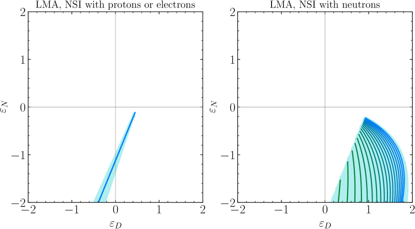
Figure 1: Departure from the adiabatic regime in presence of NSI, for a solar mixing angle in the LMA region. The pale blue regions show the values of NSI parameters leading to $\gamma^{-1}>1$, obtained from a numerical computation. The coloured lines show the values of NSI parameters where Eqs. (35) are satisfied at some point along the neutrino trajectory, for a neutrino produced at the center of the Sun. The different lines in the right panel correspond to neutrino energies between 1 MeV (green lines, at the left edge of the region) and 20 MeV (blue lines, towards the right edge).

In our past study Esteban:2018ppq , where only NSI with quarks were considered, neutrino evolution in the Sun was based on a fully numerical approach. In the present work, however, exploring the full parameter space of the most general NSI with protons, electrons, and neutrons without assuming adiabaticity is challenging from the numerical point of view. To overcome this problem in our calculations we start by evaluating the adiabaticity index for the point in the NSI and oscillation parameter space to be surveyed. If for that point $\gamma^{-1}(x)<1$ along the whole neutrino trajectory in the Sun we use the adiabatic approximation when computing the corresponding flavour transition probabilities and the subsequent prediction for all observables and $\chi^{2}$ value. If, on the contrary, the adiabaticity condition is violated somewhere inside the Sun such point is removed from the parameter space to be surveyed. We do so because we have verified that for parameter values for which adiabaticity in the Sun is violated the predicted observables with the properly computed flavour transition probability without assuming adiabaticity never lead to good description of the data. But we also find that if one evaluates the probabilities for those parameters wrongly using the adiabatic approximation, one can find a “fake” good fit to the Solar and KamLAND data, which would lead to wrong conclusions about their acceptability. In conclusion, the adiabatic approximation can be safely used for the purposes of this work as long as one removes from the parameter space those points for which adiabaticity in the Sun is violated. Furthermore, once the data of atmospheric neutrino experiments is added to the fit, it totally disfavors the parameter regions where transitions in the Sun are not adiabatic.

2.2 Neutrino detection cross sections in the presence of NSI

In addition to propagation effects discussed above, non-standard interactions can also affect scattering in the detector. In this respect, it should be mentioned that all the atmospheric, reactor and accelerator experiments included in our fit rely on CC processes in order to detect neutrinos, so the corresponding cross-section is not affected by the NC-like NSI considered here. This implies that the $\sigma^{\text{det}}$ generalized cross-section matrix entering Eq. (9) is diagonal in the SM flavour basis, and its non-zero entries coincide with the usual SM cross-section, that is,

$$\sigma^{\text{det}}=\operatorname{diag}(\sigma_{e}^{\text{SM}},\,\sigma_{\mu}^{\text{SM}},\,\sigma_{\tau}^{\text{SM}})\,\qquad\text{for CC processes.}$$ (36)

Some solar neutrino experiments, on the contrary, are sensitive to NC NSI in some of the detection processes involved. This is the case of Borexino and SK (and SNO, albeit with lower sensitivity) which observe neutrino-electron ES, which may be affected by electron NSI. Regarding NSI with nuclei SNO can also probe axial-vector NSI in NC events, and CE$\nu$NS experiments are able to set important constraints on vector interactions. In the rest of this section we review the phenomenological implications for these three cases separately.

2.2.1 Neutrino-electron elastic scattering

The presence of flavour-changing effects in NSI implies that the SM flavour basis no longer coincides with the interaction eigenstates of the neutrino-electron scattering. In such case the generalized cross section $\sigma^{\text{det}}$ can be obtained as the integral over the electron recoil kinetic energy $T_{e}$ of the following matrix expression:

$$\dfrac{\mathrm{d}\sigma^{\text{ES}}}{\mathrm{d}T_{e}}(E_{\nu},T_{e})=\dfrac{2G_{F}^{2}m_{e}}{\pi}\bigg{\{}C_{L}^{2}\Big{[}1+\dfrac{\alpha}{\pi}f_{-}(y)\Big{]}+C_{R}^{2}\,(1-y)^{2}\Big{[}1+\dfrac{\alpha}{\pi}f_{+}(y)\Big{]}\\ -\big{\{}C_{L},C_{R}\big{\}}\,\dfrac{m_{e}y}{2E_{\nu}}\Big{[}1+\dfrac{\alpha}{\pi}f_{\pm}(y)\Big{]}\bigg{\}}$$ (37)

where $y\equiv T_{e}/E_{\nu}$ and $f_{+}$, $f_{-}$, $f_{\pm}$ are loop functions given in Ref. Bahcall:1995mm , while $\alpha$ stands for the fine-structure constant and $m_{e}$ is the electron mass. In this formula $C_{L}$ and $C_{R}$ are $3\times 3$ hermitian matrices which incorporate both SM and NSI contributions:

$$C_{\alpha\beta}^{L}\equiv c_{L\beta}\,\delta_{\alpha\beta}+\varepsilon_{\alpha\beta}^{e,L}\quad\text{and}\quad C_{\alpha\beta}^{R}\equiv c_{R\beta}\,\delta_{\alpha\beta}+\varepsilon_{\alpha\beta}^{e,R}\,.$$ (38)

The effective couplings $c_{L\beta}$ and $c_{R\beta}$ account for the SM part, and contain both the flavour-universal NC terms and the $\nu_{e}$-only CC scattering:

$$c_{Le} =\rho\,\Big{[}\kappa_{e}(T_{e})\sin^{2}\theta_{w}-\dfrac{1}{2}\Big{]}+1\,, \quad c_{Re} =\rho\,\kappa_{e}(T_{e})\sin^{2}\theta_{w}\,,$$ (39)

$$c_{L\tau}=c_{L\mu} =\rho\,\Big{[}\kappa_{\mu}(T_{e})\sin^{2}\theta_{w}-\dfrac{1}{2}\Big{]}\,, \quad c_{R\tau}=c_{R\mu} =\rho\,\kappa_{\mu}(T_{e})\sin^{2}\theta_{w}\,,$$

with $\theta_{w}$ being the weak mixing angle, and $\rho$ and $\kappa_{\beta}(T_{e})$ departing from $1$ due to radiative corrections of the gauge boson self-energies and vertices Bahcall:1995mm . It is immediate to see that, if the NSI terms $\varepsilon_{\alpha\beta}^{e,L}$ and $\varepsilon_{\alpha\beta}^{e,R}$ are set to zero, the matrix $\mathrm{d}\sigma^{\text{ES}}\big{/}\mathrm{d}T_{e}$ becomes diagonal. Imposing the factorization of Eq. (4) for the vector ($+$) and axial-vector ($-$) NSI we get:

$$\varepsilon_{\alpha\beta}^{e,V(A)}=\varepsilon_{\alpha\beta}^{e,L}\pm\varepsilon_{\alpha\beta}^{e,R}=\varepsilon_{\alpha\beta}\,\xi^{e}\,(\chi^{L}\pm\chi^{R})=\sqrt{5}\cos\eta\sin\zeta\,(\chi^{L}\pm\chi^{R})\,\varepsilon_{\alpha\beta}\,.$$ (40)

Let us finalize this section by discussing briefly the impact that the inclusion of NSI effects on ES could have on the generalized mass-ordering degeneracy discussed in Sec. 2.1. We have seen that the parameter transformations (14) and (20) lead to a complex conjugation of the neutrino density matrix, $\rho^{\text{det}}\to[\rho^{\text{det}}]^{*}$. As shown in Eq. (10), this does not affect the overall number of events (thus resulting in the appearance of the degeneracy) as long as it is accompanied by a similar transformation $\sigma^{\text{det}}\to[\sigma^{\text{det}}]^{*}$. The latter can be realized either as $C_{L}\to C_{L}^{*}$ and $C_{R}\to C_{R}^{*}$, which occur when both $\varepsilon_{\alpha\beta}^{e,L}$ and $\varepsilon_{\alpha\beta}^{e,R}$ undergo simple complex conjugation, or as $C_{L}\to-C_{L}^{*}$ and $C_{R}\to-C_{R}^{*}$, which require ad-hoc transformations of the diagonal entries $\varepsilon_{\alpha\alpha}^{e,L}$ and $\varepsilon_{\alpha\alpha}^{e,R}$ to compensate for the SM contribution of Eq. (39). While conceptually identical to the situation occurring in neutrino oscillations, where the extra freedom introduced by NSI allows to “flip the sign” of the standard matter effects, the specific transformations required to achieve a perfect symmetry of $\sigma^{\text{det}}$ differ from those of Eq. (20). In principle one may first choose $\varepsilon_{\alpha\beta}^{e,L}$ and $\varepsilon_{\alpha\beta}^{e,R}$ accounting for Eq. (39) and then tune $\varepsilon_{\alpha\beta}^{p,V}$ and $\varepsilon_{\alpha\beta}^{n,V}$ to fulfill Eq. (20), but this procedure is incompatible with the factorization constraint of Eq. (4), which assumes that all NSI have the same neutrino flavour structure independently of their chirality and of the charged fermion type. The net conclusion is that, for NSI involving electrons (that is, $\zeta\neq 0$) and assuming that the factorization in Eq. (4) holds, ES effects break the generalized mass-ordering degeneracy.

2.2.2 SNO neutral-current cross-section

The SNO experiment observed NC interactions of solar neutrinos on deuterium. At low energies, the corresponding cross section is dominated by the Gamow-Teller transition and it scales as $g_{A}^{2}$ where $g_{A}$ is the coupling of the neutrino current to the axial isovector hadronic current which in the SM is given by $g_{A}\equiv g_{A}^{u}-g_{A}^{d}$ Bahcall:1988em ; Bernabeu:1991sd ; Chen:2002pv . Using that the nuclear corrections to $g_{A}$ are the same when the NSI are added, we obtain that in the presence of the NC NSI we can write

$$\sigma^{\text{det}}=\sigma_{\text{SM}}\bigg{(}\frac{G_{A}}{g_{A}}\bigg{)}^{2}$$ (41)

where $G_{A}$ is an hermitian matrix in flavour space

$$\frac{G_{A}}{g_{A}}=\delta_{\alpha\beta}+\varepsilon_{\alpha\beta}^{u,A}-\varepsilon_{\alpha\beta}^{d,A}=\delta_{\alpha\beta}+\varepsilon_{\alpha\beta}\,(\xi^{u}-\xi^{d})\,(\chi^{L}-\chi^{R})\,,$$ (42)

Clearly for vector NSI ($\chi^{L}=\chi^{R}$), the NSI contributions vanish and $\sigma^{\text{det}}$ takes just the SM value times the identity in flavour space. Conversely for axial-vector NSI one gets $\chi^{L}-\chi^{R}=1$ and the NSI term contributes.

2.2.3 Coherent elastic neutrino-nucleus scattering

The generalized cross-section $\sigma^{\text{det}}$ describing CE$\nu$NS in the presence of NSI can be obtained by integrating over the recoil energy of the nucleus $E_{R}$ the following expression:

$$\frac{\mathrm{d}\sigma^{\text{coh}}(E_{R},E_{\nu})}{\mathrm{d}E_{R}}=\frac{G_{F}^{2}}{2\pi}\,\mathcal{Q}^{2}\,F^{2}(q^{2})\,m_{A}\bigg{(}2-\frac{m_{A}E_{R}}{E_{\nu}^{2}}\bigg{)}$$ (43)

where $m_{A}$ is the mass of the nucleus and $F(q^{2})$ is its nuclear form factor evaluated at the squared momentum transfer of the process, $q^{2}=2m_{A}E_{R}$. In this formalism, the structure in flavour space which characterizes $\sigma^{\text{det}}$ is encoded into the hermitian matrix $\mathcal{Q}$, which is just the generalization of the weak charge of the nucleus for this formalism. For a nucleus with $Z$ protons and $N$ neutrons, it reads:

$$\mathcal{Q}_{\alpha\beta}=Z\big{(}g_{p}^{V}\delta_{\alpha\beta}+\varepsilon_{\alpha\beta}^{p,V}\big{)}+N\big{(}g_{n}^{V}\delta_{\alpha\beta}+\varepsilon_{\alpha\beta}^{n,V}\big{)}$$ (44)

where $g_{p}^{V}=1/2-2\sin^{2}\theta_{w}$ and $g_{n}^{V}=-1/2$ are the SM vector couplings to protons and neutrons, respectively. In experiments with very short baselines such as those performed so far, neutrinos have no time to oscillate and therefore the density matrix at the detector $\rho^{\text{det}}$ is just the identity matrix. Taking this explicitly into account in Eq. (9) we get:

$$\rho^{\text{det}}=I\quad\Rightarrow\quad N_{\text{ev}}\propto\mathcal{Q}_{\alpha}^{2}\quad\text{with}\quad\mathcal{Q}_{\alpha}^{2}\equiv\big{[}\mathcal{Q}^{2}\big{]}_{\alpha\alpha}=(\mathcal{Q}_{\alpha\alpha})^{2}+\sum_{\beta\neq\alpha}|\mathcal{Q}_{\alpha\beta}|^{2}$$ (45)

for incident neutrino flavour $\alpha$, thus recovering the expressions for the ordinary weak charges $\mathcal{Q}_{\alpha}^{2}$ used in our former publications. Coming back to Eq. (44), let us notice that it can be rewritten as:

$$\mathcal{Q}_{\alpha\beta}=Z\big{[}(g_{p}^{V}+Y_{n}^{\text{coh}}g_{n}^{V})\,\delta_{\alpha\beta}+\varepsilon_{\alpha\beta}^{\text{coh}}\big{]}\quad\text{with}\quad\varepsilon_{\alpha\beta}^{\text{coh}}\equiv\varepsilon_{\alpha\beta}^{p,V}+Y_{n}^{\text{coh}}\varepsilon_{\alpha\beta}^{n,V}$$ (46)

where $Y_{n}^{\text{coh}}\equiv N/Z$ is the neutron/proton ratio characterizing the target of a given CE$\nu$NS experiment. Imposing the quark-lepton factorization of Eq. (4) we get:

$$\varepsilon_{\alpha\beta}^{\text{coh}}=\varepsilon_{\alpha\beta}\big{(}\xi^{p}+Y_{n}^{\text{coh}}\xi^{n}\big{)}\big{(}\chi^{L}+\chi^{R}\big{)}=\sqrt{5}\,\big{[}\!\cos\eta\,\cos\zeta+Y_{n}^{\text{coh}}\sin\eta\big{]}\big{(}\chi^{L}+\chi^{R}\big{)}\,\varepsilon_{\alpha\beta}\,.$$ (47)

Similarly to Eq. (22), this expression suggests that the analysis of coherent scattering data can be performed in terms of the effective couplings $\varepsilon_{\alpha\beta}^{\text{coh}}$, whose best-fit value and allowed ranges are independent of $(\eta,\zeta)$. As a consequence, the bounds on $\varepsilon_{\alpha\beta}$ simply scale as $[\cos\eta\cos\zeta+Y_{n}^{\text{coh}}\sin\eta]$. In analogy to Eq. (19), one can define an effective angle $\tan\eta^{\prime\prime}\equiv\tan\eta\,\big{/}\cos\zeta$ parametrizing the direction in the $(\xi^{p},\xi^{n})$ plane, such that all CE$\nu$NS experiments depend on $(\eta,\zeta)$ only thought the combination $\eta^{\prime\prime}$. In particular, it is straightforward to see that a coherent scattering experiment characterized by a given $Y_{n}^{\text{coh}}$ ratio will yield no bound on $\varepsilon_{\alpha\beta}$ for $\eta^{\prime\prime}=\arctan(-1/Y_{n}^{\text{coh}})$, as for this value the effects of NSI on protons and neutrons cancel exactly. Such a cancellation can be obtained, for example, for models of the type proposed in Ref. Bernal:2022qba , where the $Z^{\prime}$ associated to a new gauge symmetry also has a sizable kinetic mixing with the SM photon, which allows for arbitrary relative size of NSI with up and down quarks.

3 Results

This section summarizes the main results of our study. In Sec. 3.1 we first review the data included in the fit, introduce our $\chi^{2}$ definition, and outline the details related to the sampling of the multi-dimensional parameter space. We then proceed to present our results for NSI with electrons (Sec. 3.2), with quarks (Sec. 3.3), and for simultaneous NSI with electrons and quarks (Sec. 3.4). The status of the LMA-D solution in this general case is discussed in Sec. 3.5.

3.1 Simulation details

The data samples included in our oscillation analysis mostly coincide with those in NuFIT-5.2 nufit-5.2 . In brief, in the analysis of solar neutrino data we consider the total rates from the radiochemical experiments Chlorine Cleveland:1998nv , Gallex/GNO Kaether:2010ag , and SAGE Abdurashitov:2009tn , the spectral data (including day-night information) from the four phases of Super-Kamkoikande in Refs. Hosaka:2005um ; Cravens:2008aa ; Abe:2010hy ; SK:nu2020 , the results of the three phases of SNO in the form of the day-night spectrum data of SNO-I Aharmim:2007nv , and SNO-II Aharmim:2005gt and the three total rates of SNO-III Aharmim:2008kc , and the spectra from Borexino Phase-I Bellini:2011rx ; Bellini:2008mr , and Phase-II Borexino:2017rsf . For reactor neutrinos we include the separate DS1, DS2, DS3 spectra from KamLAND Gando:2013nba with Daya Bay reactor $\nu$ fluxes An:2016srz , the FD/ND spectral ratio, with 1276-day (FD), 587-day (ND) exposures of Double-Chooz DoubleC:nu2020 , the 3158-day separate EH1, EH2, EH3 spectra DayaBay:2022orm of Daya-Bay, and the 2908-day FD/ND spectral ratio of RENO RENO:nu2020 . For atmospheric neutrinos we use the four phases of Super-Kamiokande (up to 1775 days of SK4 Wendell:2014dka ), the complete set of DeepCore 3-year $\mu$-like events presented in Ref. Aartsen:2014yll and publicly released in Ref. deepcore:2016 , and the results on $\nu_{\mu}$-induced upgoing muons reported by IceCube TheIceCube:2016oqi based on one year of data taking. Finally, for LBL experiments we include the final neutrino and antineutrino spectral data on $\nu_{e}$-appearance and $\nu_{\mu}$-disappearance in MINOS Adamson:2013whj , the $19.7\times 10^{20}$ pot $\nu_{\mu}$-disappearance and $16.3\times 10^{20}$ pot $\bar{\nu}_{\mu}$-disappearance data in T2K T2K:nu2020 , and the $13.6\times 10^{20}$ pot $\nu_{\mu}$-disappearance and $12.5\times 10^{20}$ pot $\bar{\nu}_{\mu}$-disappearance data in NO$\nu$A NOvA:nu2020 . Notice that to ensure full consistency with our CP-conserving parametrization we have chosen not to include in the present study the data from the $\nu_{e}$ and $\bar{\nu}_{e}$ appearance channels in NO$\nu$A and T2K. With this data we construct $\chi^{2}_{\text{OSC}}(\vec{\omega},\vec{\varepsilon})$ where we denote by $\vec{\omega}$ the 3$\nu$ oscillation parameters and $\vec{\varepsilon}$ the NSI parameters considered in the analysis.

When combining with CE$\nu$NS we include the results from COHERENT data on CsI COHERENT:2017ipa ; COHERENT:2018imc and Ar targets COHERENT:2020iec ; COHERENT:2020ybo (see Refs. Coloma:2019mbs ; Coloma:2022avw for details). In particular, for the analysis of COHERENT CsI data we use the quenching factor from Ref. Collar:2019ihs and the nuclear form factor from Ref. Klos:2013rwa . For the analysis of COHERENT Ar data we use the quenching factor provided by the COHERENT collaboration in Ref. COHERENT:2020ybo and Helm Helm:1956zz nuclear form factor (the values of the parameters employed are the same as in Ref. Coloma:2022avw ). For CE$\nu$NS searches using reactor neutrinos at Dresden-II reactor experiment Colaresi:2022obx we follow the analysis presented in Ref. Coloma:2022avw with YBe quenching factor Collar:2021fcl (the characteristic momentum-transfer in this experiment is very low so the nuclear form factor can be taken to be 1). With all this we construct the corresponding $\chi^{2}_{\text{COH,CsI}}(\vec{\varepsilon})$, $\chi^{2}_{\text{COH,Ar}}(\vec{\varepsilon})$, and $\chi^{2}_{\text{D-II,Ge}}(\vec{\varepsilon})$.

Our goal is to find the global minimum of the total $\chi^{2}$ which, unless otherwise stated, is obtained adding the contributions from our global analysis of oscillation data (<<GLOB-OSC w NSI in ES>>) and CE$\nu$NS data:

$$\chi^{2}(\vec{\omega},\vec{\varepsilon})=\chi^{2}_{\text{OSC}}(\vec{\omega},\vec{\varepsilon})+\chi^{2}_{\text{CE$\nu$NS}}(\vec{\varepsilon})$$ (48)

where we have defined

$$\chi^{2}_{\text{CE$\nu$NS}}=\chi^{2}_{\text{COH,CsI}}+\chi^{2}_{\text{COH,Ar}}+\chi^{2}_{\text{D-II,Ge}}\,.$$ (49)

The minimum of the total $\chi^{2}$ is obtained after minimization over all the nuisance parameters, which are included as pull terms in our fit. However, note that a priori it is possible to suppress the effects of vector NSI in neutrino detection while still allowing for sizable NSI in oscillations, since the momentum transfer required for the effects to be observable is not the same in the two cases Farzan:2015doa . The paradigmatic example of BSM scenarios leading to sizable NSI are models with light mediators. Matter effects arise from a coherent effect, that is, with zero momentum-transfer, and therefore apply to NSI induced by ultra light mediators, as long as their mass is $M_{\text{med}}\gtrsim 1/R_{\oplus}\sim\mathcal{O}(10^{-12})$ eV Gonzalez-Garcia:2006vp ; Coloma:2020gfv . Scattering effects, on the contrary, require a minimum momentum-transfer to be observable:

• In the case of ES, for recoil energies $T_{e}\simeq\mathcal{O}(500~{}\text{keV})$ (which are in the right ballpark for Borexino) the relevant scale is $q=\sqrt{2m_{e}T_{e}}\sim\mathcal{O}(500~{}\text{keV})$. Therefore, in what follows we will also present our results neglecting the effects due to NSI in detection (<<GLOB-OSC w/o NSI in ES>>), so as to consider this class of models with very light mediators, $M_{\text{med}}\ll\mathcal{O}(500~{}\text{keV})$. For SNO and SK, sensitive to neutrinos with higher energies, a similar argument leads to $q\sim\mathcal{O}(5-10~{}\text{MeV})$. Hence, results labeled as <<GLOB-OSC w NSI in ES>> apply to NSI generated by models with $M_{\text{med}}\gtrsim 10~{}\text{MeV}$, where we expect to have NSI effects on the detection through ES for all solar experiments considered in this work. Finally, in the intermediate mass range only Borexino would be fully sensitive to NSI effects on detection.

• In the case of CE$\nu$NS, the relevant momentum transfer also depends on the experiment considered. For COHERENT data on CsI (Ar), this can be estimated as $q\sim 50~{}\text{MeV}$ ($q\sim 30~{}\text{MeV}$) while for Dresden-II we get $q\sim\mathcal{O}(5~{}\text{MeV})$. Therefore, in Sec. 3.3 we will present our results using the combination of all oscillation and CE$\nu$NS data, sensitive to models with $M_{\text{med}}\gtrsim 50~{}\text{MeV}$ (<<GLOB-OSC+CE$\nu$NS>>), as well as the results for oscillation data alone, sensitive to NSI models with $M_{\text{med}}\ll 5~{}\text{MeV}$ (labeled as <<GLOB-OSC>>). In the intermediate mass range between 5 and 50 MeV, effects on CE$\nu$NS may be suppressed for some experiments but not all of them.

The intermediate mass ranges defined above (where NSI effects in detection may be observed at one experiment, but not another) require special handling and are therefore beyond the scope of the present paper, leaving them for future work.

In the axial-vector case there are no NSI effects in oscillations nor CE$\nu$NS and the NSI parameters only enter in the ES and/or NC detection cross sections. Thus for axial-vector NSI with electrons the derived bounds apply for mediator masses as discussed above for ES. NC interactions in SNO occur for neutrinos with energy above the binding energy of the deuteron, 2.22 MeV. So the bounds for axial-vector NSI with quarks derived here apply for $M_{\text{med}}\gtrsim 3~{}\text{MeV}$.

Let us finalize this discussion by briefly reviewing the number of parameters involved in the fit. A priori, under the approximations assumed in the present work, atmospheric and long-baseline experiments depend on all the oscillation parameters as well as on the NSI variables defined in Eqs. (24). However, for LBL experiments we fix $\Delta m^{2}_{21}$ and $|\theta_{12}-45^{\circ}|$ to their SM best-fit value, as their relevance for such data is only subleading and we know from previous studies Esteban:2018ppq that NSI are not going to spoil their determination sizably (except for the $\theta_{12}$ octant which we do not fix, hence the absolute value in the corresponding fixed value above). For the analysis of atmospheric neutrinos we further set $\Delta m^{2}_{21}\to 0$, so the dependence on $\theta_{12}$ and $\delta_{\text{CP}}$ vanishes. With this, neutrino propagation through the Earth is described in terms of six continuous parameters, namely ($\Delta m^{2}_{31}$, $\theta_{13}$, $\theta_{23}$) for the vacuum part and ($\varepsilon_{\oplus}$, $\varphi_{12}$, $\varphi_{13}$) for the matter part, as well as the two CP-conserving values of $\delta_{\text{CP}}$ and the two options for the $\theta_{12}$ octant. We additionally fix the value of $\theta_{13}$ to the present best fit, as its determination comes mainly from reactor experiments for which NSI effects are suppressed. On the other hand, neutrino oscillations in solar and KamLAND data depend effectively on $\varepsilon_{D}$ and $\varepsilon_{N}$ for the matter part, while the vacuum part depends on $\theta_{12}$, $\theta_{23}$, $\Delta m^{2}_{21}$ and the two-CP conserving values of $\delta_{\text{CP}}$ ($\theta_{13}$ is also fixed to its best-fit value here). Finally note that, while oscillations depend on differences between the diagonal NSI parameters, the addition of scattering effects in detection breaks this pattern. This implies that in addition to the two differences in Eqs. (22) we need to scan one of the diagonal parameters, which we take to be $\varepsilon_{\mu\mu}^{\oplus}$. The last two parameters of relevance are the two angles $\eta$ and $\zeta$, which determine the direction of NSI in $(\xi^{e},\xi^{p},\xi^{n})$ space.

Taking into account all of the above, in our simulations we scan the multi-dimensional space spanned by the following continuous parameters:

$$\theta_{12},\,\theta_{23},\,\Delta m^{2}_{21},\,\Delta m^{2}_{31},\,\varepsilon_{\oplus},\,\varphi_{12},\,\varphi_{23},\,\varepsilon_{\mu\mu}^{\oplus},\,\eta,\,\zeta,$$ (50)

as well as the two CP-conserving values of $\delta_{\text{CP}}\in\{0,\pi\}$. In order to scan this multi-dimensional parameter space efficiently, we make use of the MultiNest Feroz:2013hea ; Feroz:2008xx and Diver Martinez:2017lzg algorithms.

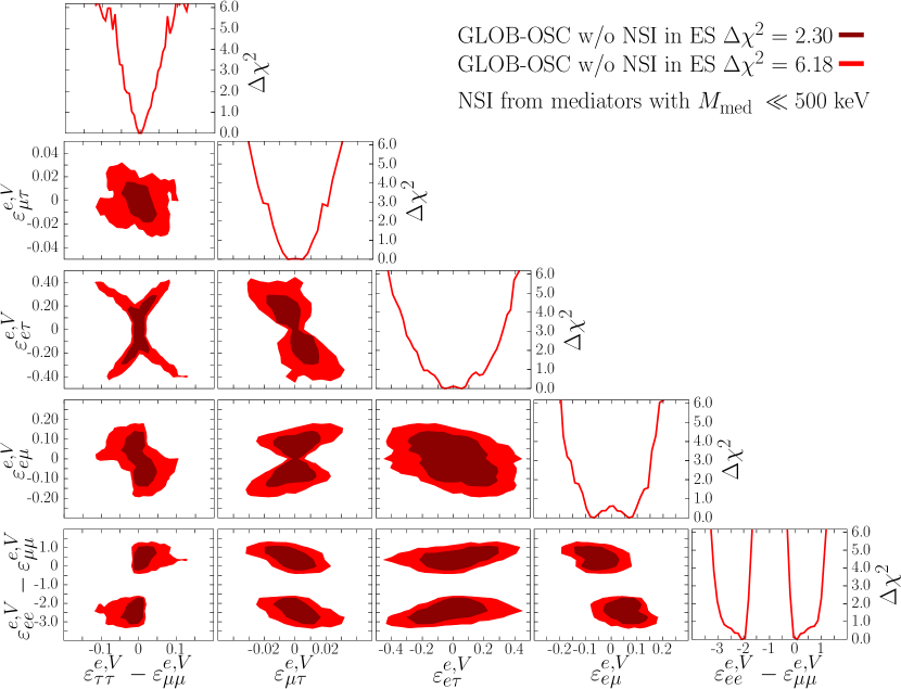
Figure 2: Constraints on the coefficients for vector NSI with electrons from the global analysis of oscillation data without including the effect of NSI in the detection cross section. Each panel shows a two-dimensional projection of the allowed multi-dimensional parameter space after minimization with respect to the undisplayed parameters. The regions correspond to $1\sigma$ and $2\sigma$ (2 d.o.f.).

	Allowed ranges at 90% CL (marginalized)
	GLOB-OSC w/o NSI in ES
	LMA	$\text{LMA}\oplus\text{LMA-D}$
$\varepsilon_{ee}^{e,V}-\varepsilon_{\mu\mu}^{e,V}$	$[-0.21,+1.0]\hphantom{0}$	$[-3.0,-1.8]\oplus[-0.21,+1.0]$
$\varepsilon_{\tau\tau}^{e,V}-\varepsilon_{\mu\mu}^{e,V}$	$[-0.015,+0.048]$	$[-0.040,+0.047]$
$\varepsilon_{e\mu}^{e,V}$	$\hphantom{0}[-0.15,+0.035]$	$[-0.15,+0.14]$
$\varepsilon_{e\tau}^{e,V}$	$[-0.21,+0.31]$	$[-0.29,+0.31]$
$\varepsilon_{\mu\tau}^{e,V}$	$[-0.020,+0.012]$	$[-0.020,+0.017]$

Table 1: 90% CL bounds (1 d.o.f., 2-sided) on the coefficients of NSI operators with electrons after marginalizing over all other NSI and oscillation parameters. The bounds are derived from the global analysis of oscillation data without including the effect of NSI in the ES cross section (NSI induced by mediators with mass $M_{\text{med}}\ll 500~{}\text{keV}$, see Sec. 3.1). The ranges in the first column (labeled <<LMA>>) correspond to an analysis in which we restrict $\theta_{12}<45^{\circ}$. In the second column (labeled <<$\text{LMA}\oplus\text{LMA-D}$>>), both $\theta_{12}<45^{\circ}$ and $\theta_{12}>45^{\circ}$ are allowed. The same bounds hold for vector NSI with protons.

3.2 New constraints on NSI with electrons

We start by describing the results of the global analysis for the case of NSI with electrons, which, as mentioned in the introduction, was not considered in our previous studies Gonzalez-Garcia:2013usa ; Esteban:2018ppq ; Coloma:2019mbs . We plot in Fig. 2 and 3 the constraints on the different coefficients for the two scenarios outlined in the previous section, without and with NSI effects in the detection cross section, respectively. The corresponding 90% CL allowed ranges are listed in Table 1 and on the left columns in Table 2 respectively.

	Allowed ranges at 90% CL (marginalized)
	Vector ($X=V$)		Axial-vector ($X=A$)
	Borexino	GLOB-OSC w NSI in ES	Borexino	GLOB-OSC w NSI in ES
$\varepsilon^{e,X}_{ee}$	$\hphantom{0}[-1.1,+0.17]$	$[-0.13,+0.10]$	$[-0.38,+0.24]$	$[-0.13,+0.11]$
$\varepsilon^{e,X}_{\mu\mu}$	$[-2.4,+1.5]$	$[-0.20,+0.10]$	$[-1.5,+2.4]$	$[-0.70,+1.2]\hphantom{0}$
$\varepsilon^{e,X}_{\tau\tau}$	$[-2.8,+2.1]$	$\hphantom{0}[-0.17,+0.093]$	$[-1.8,+2.8]$	$[-0.53,+1.0]\hphantom{0}$
$\varepsilon^{e,X}_{e\mu}$	$[-0.83,+0.84]$	$[-0.097,+0.011]$	$[-0.79,+0.76]$	$[-0.41,+0.40]$
$\varepsilon^{e,X}_{e\tau}$	$[-0.90,+0.85]$	$\hphantom{0}[-0.18,+0.080]$	$[-0.81,+0.78]$	$[-0.36,+0.36]$
$\varepsilon^{e,X}_{\mu\tau}$	$[-2.1,+2.1]$	$[-0.0063,+0.016]\hphantom{0}$	$[-1.9,+1.9]$	$[-0.79,+0.81]$

Table 2: 90% CL bounds (1 d.o.f., 2-sided) on the coefficients of vector NSI operators with electrons after marginalizing over all other NSI and oscillation parameters. The bounds are derived from the global analysis of oscillation data including the effect of NSI in the ES cross section. For comparison, the results obtained from the analysis of Borexino Phase-II data in Ref. Coloma:2022umy are also shown for comparison. Note that these bounds apply to interactions induced by mediators with masses $M_{\text{med}}\gtrsim 10~{}\text{MeV}$, see Sec. 3.1.

The first thing to notice is that in the scenario <<GLOB-OSC w/o NSI in ES>>, for the flavour diagonal coefficients, only the combinations $\varepsilon_{ee}^{e,V}-\varepsilon_{\mu\mu}^{e,V}$ and $\varepsilon_{\tau\tau}^{e,V}-\varepsilon_{\mu\mu}^{e,V}$ can be constrained, and two separate allowed ranges appear (see bottom row in Fig. 2): one around $\varepsilon_{ee}^{e,V}-\varepsilon_{\mu\mu}^{e,V}\sim 0$ and another around $\varepsilon_{ee}^{e,V}-\varepsilon_{\mu\mu}^{e,V}\sim-2$. This is nothing else than the result of the generalized mass-ordering degeneracy of Eq. (20). The two disjoint allowed solutions correspond to regions of oscillation parameters with $\theta_{12}<45^{\circ}$ (with ranges labeled <<LMA>> in Table 1) and with $\theta_{12}>45^{\circ}$ (with ranges labeled <<LMA-D>> in Table 1) respectively. As discussed in Sec. 2.1, the degeneracy is partly broken by the variation of chemical composition of the matter along the neutrino trajectory when NSI coupling to neutrons are involved. But in this case, with only coupling to electrons, the degeneracy is perfect as can be seen by the fact that $\Delta\chi^{2}=0$ in both minima of $\varepsilon_{ee}^{e,V}-\varepsilon_{\mu\mu}^{e,V}$. From the panels on the lower row we observe that the projection of the allowed regions corresponding to each of the two solutions partly overlap for $\varepsilon_{\tau\tau}^{e,V}-\varepsilon_{\mu\mu}^{e,V}$ and $\varepsilon_{\alpha\neq\beta}^{e,V}$, which leads to the non-trivial shapes of some of the corresponding two-dimensional regions for some pairs of those paremeters.

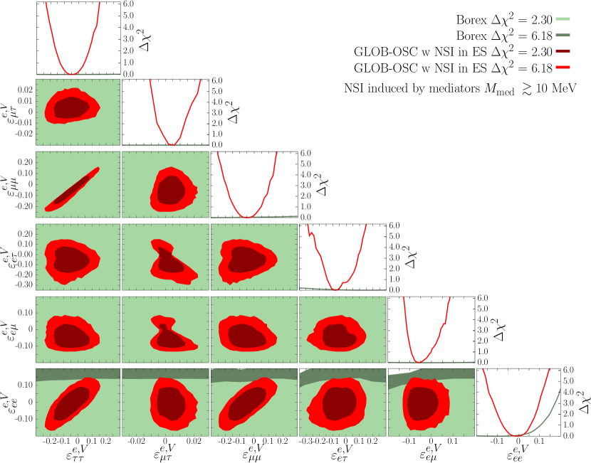
Figure 3: Constraints on the coefficients for vector NSI with electrons from the global analysis of oscillation data including the effect of NSI in the ES cross section. Each panel shows a two-dimensional projection of the allowed multi-dimensional parameter space after minimization with respect to the undisplayed parameters. The contours correspond to $1\sigma$ and $2\sigma$ (2 d.o.f.). The closed red regions correspond to the global oscillation analysis which involves the six NSI plus five oscillation parameters. For the sake of comparison we also show as green regions the constraints obtained from the analysis of full Borexino Phase-II spectrum in Ref. Coloma:2022umy .

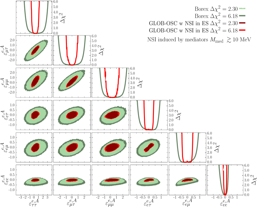
Figure 4: Same as Fig. 3 but for Axial-vector NSI.

The results for the scenario <<GLOB-OSC w NSI in ES>> in Fig. 2, and on the left columns in Table 2, show that the inclusion of the effect of the vector NSI in the ES cross sections in Borexino, SNO, and SK totally lifts the degeneracy. In this scenario only the LMA solution is allowed, and $\varepsilon_{ee}^{e,V}$, $\varepsilon_{\mu\mu}^{e,V}$, and $\varepsilon_{\tau\tau}^{e,V}$ can be independently constrained. Notice also that in this case, the lifting of the LMA-D solution leads to allowed regions with more standard (close-to-elliptical) shapes. For the sake of comparison we show for this scenario the corresponding bounds derived from the analysis of Borexino spectra in Ref. Coloma:2022umy . The comparison shows that for vector NSI with electrons the global analysis of the oscillation data reduces the allowed ranges of the NSI coefficients by factors $\sim\text{4--200}$ with respect to those derived with Borexino spectrum only. In other words, the NSI contribution to ES is important to break the LMA-D degeneracy and to impose independent bounds on the three flavour-diagonal NSI coefficients, but within the LMA solution the effect of the vector NSI on the matter potential also leads to stronger constraints. This is further illustrated by the results obtained for the analysis with axial-vector NSI which are shown in Fig. 4 and right columns in Table 2. Axial-vector NSI do not contribute to the matter potential and therefore the difference between the results of the global oscillation and the Borexino-only analysis in this case arises solely from the effect of the axial-vector NSI on the ES cross section in SNO and SK. Comparing the red and green regions in Fig. 4 and the two left columns in Table 2 we see that for axial-vector NSI the improvement over the bounds derived with Borexino-only analysis is just a factor $\sim$ 2–3.

3.3 Updated constraints on NSI with quarks

Next we briefly summarize the results of the analysis for the scenarios of NSI with either up or down quarks (more general combinations of couplings to quarks and electrons will be presented in the next section). For vector NSI this updates and complements the results presented in Refs. Esteban:2018ppq ; Coloma:2019mbs by accounting for the effects of increased statistics in the oscillation experiments, including the addition of new data from Borexino Phase-II. Notice also that in the present analysis, as mentioned above, the treatment of the SNO data is different than in Refs. Esteban:2018ppq ; Coloma:2019mbs . Furthermore when combining with CE$\nu$NS we include here the results from COHERENT both on CsI COHERENT:2017ipa ; COHERENT:2018imc and Ar targets COHERENT:2020iec ; COHERENT:2020ybo , together with the recent results from CE$\nu$NS searches using reactor neutrinos at Dresden-II reactor experiment Colaresi:2022obx ; Coloma:2022avw .

Let us start discussing the complementary sensitivity to vector-NSI from the combined CE$\nu$NS results with that from present oscillation data, for general models leading to NSI with quarks. With this aim we have first performed an analysis including only the effect of vector NSI on the matter potential in the neutrino oscillation experiments. The results of such analysis are given in the left column of Table 5 in terms of the allowed ranges of the effective NSI couplings to the Earth matter, $\varepsilon^{\oplus}_{\alpha\beta}$, defined in Eq. (21) (see Sec. 3.4 for details). Comparison with the constraints from all available CE$\nu$NS data is illustrated in Fig. 5 where we plot the allowed regions in the plane ($\varepsilon^{\oplus}_{ee}$, $\varepsilon^{\oplus}_{\mu\mu}$). The figure shows the allowed regions obtained by the analysis of each of the two sets of data independently, after marginalization over the all other (including off-diagonal) NSI parameters. As discussed in Sec. 2.2.3, even when considering NSI coupling only to quarks, there is always a value of $\eta$ for which the contribution of NSI to the CE$\nu$NS cross section cancels. Consequently CE$\nu$NS data with a single nucleus does not lead to any constraint on the $\varepsilon^{\oplus}_{\alpha\beta}$ parameters. However, the cancellation occurs at different values of $\eta$ for the three nucleus considered (CsI, Ar, and Ge), and consequently, as seen in the figure, the combination of CE$\nu$NS data with the three nuclear targets does constrain the full space of effective $\varepsilon^{\oplus}_{\alpha\beta}$, even after marginalization over $\eta$. The constraints derived from the combined CE$\nu$NS data are independent (and complementary) to those provided by the oscillation analysis and, as seen in the figure, they are fully consistent.

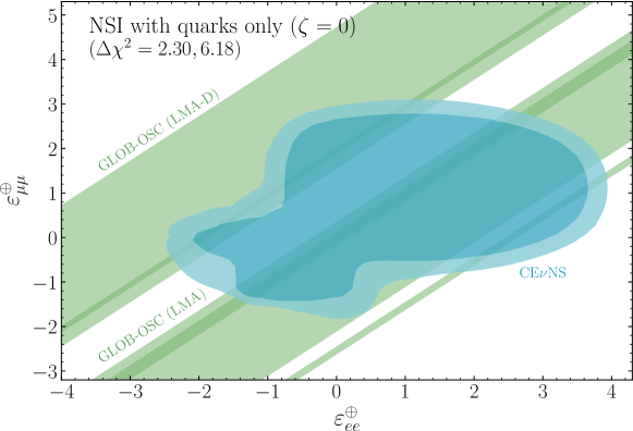
Figure 5: Allowed regions in the plane of $\varepsilon^{\oplus}_{ee}$ and $\varepsilon^{\oplus}_{\mu\mu}$ for vector NSI with quarks from the combinations of CE$\nu$NS data compared with the allowed regions from the global oscillation analysis which are the two diagonal shaded bands corresponding to the LMA and LMA-D solutions. Both the green and blue regions are obtained after independently marginalizing over all other relevant parameters: NSI couplings (including $\eta$) for the CE$\nu$NS region, and NSI couplings, $\eta$ and oscillation parameters for the <<GLOB-OSC>> regions. So the values of other NSI and $\eta$ in the blue and green regions are not forced to be the same.

The allowed ranges for vector NSI with up or down quarks are compiled in Table 3 and show good qualitative agreement with those of Refs. Esteban:2018ppq ; Coloma:2019mbs , with the expected small deviations due to the differences in the analysis, quoted CL, and included data.

	Allowed ranges at 90% CL (marginalized)			Allowed ranges at 90% CL (marginalized)
	GLOB-OSC			GLOB-OSC+CE$\nu$NS
	LMA	$\text{LMA}\oplus\text{LMA-D}$		$\text{LMA}=\text{LMA}\oplus\text{LMA-D}$
$\varepsilon_{ee}^{u,V}-\varepsilon_{\mu\mu}^{u,V}$ $\varepsilon_{\tau\tau}^{u,V}-\varepsilon_{\mu\mu}^{u,V}$	$[-0.063,+0.36]\hphantom{0}$ $[-0.0053,+0.017]\hphantom{0}$	$[-1.1,-0.79]\oplus[-0.063,+0.36]$ $[-0.021,+0.018]$	$\varepsilon_{ee}^{u,V}$ $\varepsilon_{\mu\mu}^{u,V}$ $\varepsilon_{\tau\tau}^{u,V}$	$[-0.038,+0.034]\oplus[+0.34,+0.42]$ $[-0.046,+0.031]\oplus[+0.35,+0.42]$ $[-0.046,+0.033]\oplus[+0.35,+0.42]$
$\varepsilon_{e\mu}^{u,V}$	$[-0.057,+0.013]$	$[-0.057,+0.061]$	$\varepsilon_{e\mu}^{u,V}$	$\hphantom{0}[-0.044,+0.0049]$
$\varepsilon_{e\tau}^{u,V}$	$[-0.076,+0.11]\hphantom{0}$	$[-0.12,+0.11]$	$\varepsilon_{e\tau}^{d,V}$	$[-0.079,+0.11]\hphantom{0}$
$\varepsilon_{\mu\tau}^{u,V}$	$[-0.0077,+0.0042]$	$[-0.0077,+0.0083]$	$\varepsilon_{\mu\tau}^{u,V}$	$[-0.0064,0.0053]$
$\varepsilon_{ee}^{d,V}-\varepsilon_{\mu\mu}^{d,V}$ $\varepsilon_{\tau\tau}^{d,V}-\varepsilon_{\mu\mu}^{d,V}$	$[-0.069,+0.38]\hphantom{0}$ $[-0.0058,+0.018]\hphantom{0}$	$\hphantom{0}[-1.3,-0.91]\oplus[-0.072,+0.38]\hphantom{0}$ $[-0.029,+0.019]$	$\varepsilon_{ee}^{d,V}$ $\varepsilon_{\mu\mu}^{d,V}$ $\varepsilon_{\tau\tau}^{d,V}$	$[-0.036,+0.031]\oplus[+0.30,+0.39]$ $[-0.040,+0.038]\oplus[+0.31,+0.39]$ $[-0.041,+0.043]\oplus[+0.31,+0.39]$
$\varepsilon_{e\mu}^{d,V}$	$[-0.058,+0.014]$	$[-0.058,+0.098]$	$\varepsilon_{e\mu}^{d,V}$	$\hphantom{0}[-0.054,+0.0045]$
$\varepsilon_{e\tau}^{d,V}$	$[-0.079,+0.11]\hphantom{0}$	$[-0.16,+0.11]$	$\varepsilon_{e\tau}^{d,V}$	$[-0.051,+0.11]\hphantom{0}$
$\varepsilon_{\mu\tau}^{d,V}$	$[-0.0087,+0.0051]$	$[-0.0087,+0.015]\hphantom{0}$	$\varepsilon_{\mu\tau}^{d,V}$	$[-0.0075,+0.0046]$

Table 3: 90% allowed ranges for the vector NSI couplings $\varepsilon_{\alpha\beta}^{u,V}$ and $\varepsilon_{\alpha\beta}^{d,V}$ as obtained from the global analysis of oscillation data (left columns, applicable to NSI induced by mediators with $M_{\text{med}}\ll 5~{}\text{MeV}$) and also including data from CE$\nu$NS experiments (right columns, applicable to NSI induced by mediators with $M_{\text{med}}\gtrsim 50~{}\text{MeV}$). The results are obtained after marginalizing over oscillation and the other matter potential parameters either within the LMA only ($\theta_{12}<45^{\circ}$) and within both LMA ($\theta_{12}<45^{\circ}$) and LMA-D ($\theta_{12}>45^{\circ}$) subspaces respectively (this second case is denoted as $\text{LMA}\oplus\text{LMA-D}$). Notice that once CE$\nu$NS data is included the two columns become identical, since for NSI couplings with $f=u,d$ the LMA-D solution is only allowed well above 90% CL.

Finally for completeness we have also performed a new dedicated analysis including axial-vector NSI with up or down quarks. Axial-vector NSI with quarks do not contribute to matter effects nor to CE$\nu$NS. They only enter the global analysis via their modification of the NC event rate in the SNO experiment (see Sec. 2.2.2), which is not able to constrain the NSI coefficients if all of them are included simultaneously due to possible cancellations between their respective contributions to the NC rate. Thus in this case we derive the bounds assuming that only one NSI coupling is different from zero at a time. The corresponding allowed ranges can be found in Table 4.

As seen in the table, for all the coefficients, the allowed range is composed of several disjoint intervals. They correspond to values of the NSI couplings for which the SNO-NC event rate is approximately the SM prediction. This can occur for either flavour diagonal or flavour non-diagonal coeficients because solar neutrinos reach the Earth as mass eigenstates, so the density matrix describing the neutrino state at the detector is diagonal in the mass basis, but not in the flavor basis. The presence of non-vanishing off-diagonal $\rho_{\alpha\neq\beta}$ elements is responsible for the sensitivity to off-diagonal $\varepsilon_{\alpha\neq\beta}$ coefficients. More quantitatively, the ranges correspond to coefficients verifying:

$$0\simeq\operatorname{Tr}\Bigg{[}\rho^{\text{SNO}}\,\bigg{(}\frac{G_{A}}{g_{A}}\bigg{)}^{2}\Bigg{]}-1=\left\{\begin{array}[]{l}\rho_{\alpha\alpha}^{\text{SNO}}\big{[}\big{(}\varepsilon^{q,A}_{\alpha\alpha}\big{)}^{2}\pm 2\,\varepsilon^{q,A}_{\alpha\alpha}\big{]}\,,\\[5.69054pt] \big{(}\rho^{\text{SNO}}_{\alpha\alpha}+\rho^{\text{SNO}}_{\beta\beta}\big{)}\,\big{(}\varepsilon^{q,A}_{\alpha\neq\beta}\big{)}^{2}\pm 4\mathop{\mathrm{Re}}\!\big{(}\rho^{\text{SNO}}_{\alpha\neq\beta}\big{)}\,\varepsilon^{q,A}_{\alpha\neq\beta}\end{array}\right.$$ (51)

where the upper line holds when the NSI coefficient included is flavour diagonal, and the lower one when it is flavour-changing and the $\pm$ sign correspond to $q=u$ and $q=d$ respectively. Thus the allowed range for flavour diagonal NSI is formed by two solutions around $\varepsilon_{\alpha\alpha}^{q,A}=0$ and $\varepsilon_{\alpha\alpha}^{q,A}=-2$. For flavour off-diagonal NSI it is formed by solutions around $\varepsilon_{\alpha\neq\beta}^{q,A}=0$ and $\varepsilon_{\alpha\neq\beta}^{q,A}=\mp 4\mathop{\mathrm{Re}}(\rho^{\text{SNO}}_{\alpha\neq\beta})\mathbin{\big{/}}(\rho^{\text{SNO}}_{\alpha\alpha}+\rho^{\text{SNO}}_{\beta\beta})$. For $\varepsilon^{q,A}_{e\mu}$ (and similarly for $\varepsilon^{q,A}_{e\tau}$) this last condition corresponds, in fact, to two distinct solutions, both around $|\varepsilon^{q,A}_{e\mu}|\neq 0$ and two possible signs, due to the two different signs of $\rho^{\text{SNO}}_{e\mu}$ for the two CP-conserving values of $\delta_{\text{CP}}\in\{0,\pi\}$. On the contrary, $\rho^{\text{SNO}}_{\mu\tau}$ takes very similar values for $\delta_{\text{CP}}\in\{0,\pi\}$, and consequently for $\varepsilon^{q,A}_{\mu\tau}$ the two non-zero solutions closely overlap around $\varepsilon^{u,A}_{\mu\tau}\sim 1.7$ ($\varepsilon^{d,A}_{\mu\tau}\sim-1.7$).

	Allowed ranges at 90% CL (1-parameter)
	GLOB-OSC
$\varepsilon^{u,A}_{ee}$	$\hphantom{0}\hphantom{0}[-2.1,-1.8]\oplus[-0.19,+0.13]$	$-\varepsilon^{d,A}_{ee}$
$\varepsilon^{u,A}_{\mu\mu}$	$\hphantom{0}\hphantom{0}[-2.2,-1.7]\oplus[-0.26,+0.18]$	$-\varepsilon^{d,A}_{\mu\mu}$
$\varepsilon^{u,A}_{\tau\tau}$	$\hphantom{0}\hphantom{0}[-2.1,-1.8]\oplus[-0.20,+0.15]$	$-\varepsilon^{d,A}_{\tau\tau}$
$\varepsilon^{u,A}_{e\mu}$	$[-1.5,-1.2]\oplus[-0.16,+0.12]\oplus[+1.4,+1.7]$	$-\varepsilon^{d,A}_{e\mu}$
$\varepsilon^{u,A}_{e\tau}$	$[-1.5,-1.3]\oplus[-0.13,+0.10]\oplus[+1.4,+1.7]$	$-\varepsilon^{d,A}_{e\tau}$
$\varepsilon^{u,A}_{\mu\tau}$	$[-0.085,+0.11]\oplus[+1.6,+1.9]\hphantom{0}\hphantom{0}\hphantom{0}$	$-\varepsilon^{d,A}_{\mu\tau}$

Table 4: 90% CL bounds (1 d.o.f., 2-sided) on the effective axial-vector NSI couplings with quarks. The bounds are derived from the global analysis of oscillation data including the effect of NSI in the SNO NC cross section and assuming only one NSI coupling different from zero at a time. As explained in Sec. 3.1, these bounds apply to models with $M_{\text{med}}\gtrsim 3~{}\text{MeV}$.

3.4 Constraints on NSI with quarks and electrons: effective NSI in the Earth

Let us now discuss the most general case in which NSI with quarks and electrons are considered, parametrized by the angles $\eta$ and $\zeta$ introduced in Eqs. (7) and (8). We focus on vector NSI because in this case the interplay between matter and scattering effects, and therefore the dependence on the couplings to charged fermions involved, is expected to play a most relevant role.

In this framework, it is useful to quantify the results of our analysis in terms of the effective NSI parameters which describe the generalized Earth matter potential, which are in fact the relevant quantities for the study of long-baseline and atmospheric oscillation experiments. The results are displayed in Fig. 6 and on the right column in Table 5 where we show the allowed two-dimensional regions and one-dimensional ranges of the effective NSI coefficients for the global analysis of oscillation and CE$\nu$NS data, after marginalizing over all other parameters. Therefore what we quantify in Fig. 6 and the right column in Table 5 is our present knowledge of the matter potential for neutrino propagation in the Earth, for NSI induced by mediators heavier than $M_{\text{med}}\gtrsim 50~{}\text{MeV}$ (as discussed in Sec. 3.1) and for any unknown value of $\eta$ and $\zeta$. Technically this is obtained by marginalizing the results of the global $\chi^{2}$ with respect to $\eta$ and $\zeta$ as well, and the $\Delta\chi^{2}$ functions plotted in the figure are defined with respect to the absolute minimum for any $\eta$ and $\zeta$ which, lies close to $\eta\sim-45^{\circ}$ and $\zeta\sim 10^{\circ}$.

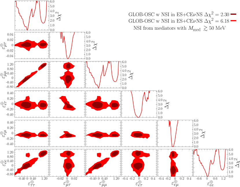
Figure 6: Constraints on the effective generalized NSI in the Earth matter (relevant for matter effects in LBL experiments) with arbitrary values of $\eta$ and $\zeta$. Each panel shows a two-dimensional projection of the allowed multi-dimensional parameter space after minimization with respect to the undisplayed parameters. The contours correspond to $1\sigma$ and $2\sigma$ (2 d.o.f.).

Allowed ranges at $90\%~{}\text{CL}$ $\big{(}99\%~{}\text{CL}\big{)}$ marginalized
GLOB-OSC w/o NSI in ES	GLOB-OSC w NSI in ES + CE$\nu$NS
$\varepsilon^{\oplus}_{ee}-\varepsilon^{\oplus}_{\mu\mu}$ $[-3.1,-2.8]\oplus[-2.1,-1.88]\oplus[-0.15,+0.17]$ $\big{(}[-4.8,-1.6]\oplus[-0.40,+2.6]\big{)}$ $\varepsilon^{\oplus}_{\tau\tau}-\varepsilon^{\oplus}_{\mu\mu}$ $[-0.0215,+0.0122]$ $\big{(}[-0.075,+0.080]\big{)}$ $\varepsilon^{\oplus}_{e\mu}$ $[-0.11,-0.021]\oplus[+0.045,+0.135]$ $\big{(}[-0.32,+0.40]\big{)}$ $\varepsilon^{\oplus}_{\mu\tau}$ $[-0.22,+0.088]$ $\big{(}[-0.49,+0.45]\big{)}$ $\varepsilon^{\oplus}_{\mu\tau}$ $[-0.0063,+0.013]$ $\big{(}[-0.043,+0.039]\big{)}$	$\varepsilon^{\oplus}_{ee}$ $[-0.19,+0.20]\oplus[+0.95,+1.3]$ $\big{(}[-0.23,+0.25]\oplus[+0.81,+1.3]\big{)}$ $\varepsilon^{\oplus}_{\mu\mu}$ $[-0.43,+0.14]\oplus[+0.91,+1.3]$ $\big{(}[-0.29,+0.20]\oplus[+0.83,+1.4]\big{)}$ $\varepsilon^{\oplus}_{\tau\tau}$ $[-0.43,+0.14]\oplus[+0.91,+1.3]$ $\big{(}[-0.29,+0.20]\oplus[+0.83,+1.4]\big{)}$ $\varepsilon_{e\mu}^{\oplus}$ $[-0.12,+0.011]$ $\big{(}[-0.18,+0.08]\big{)}$ $\varepsilon_{e\tau}^{\oplus}$ $[-0.16,+0.083]$ $\big{(}[-0.25,+0.33]\big{)}$ $\varepsilon_{\mu\tau}^{\oplus}$ $[-0.0047,+0.012]$ $\big{(}[-0.020,+0.021]\big{)}$

Table 5: 90% and 99% CL bounds (1 d.o.f., 2-sided) on the effective NSI parameters relevant for matter effects in LBL experiments with arbitrary values of $\eta$ and $\zeta$, obtained after marginalizing over all other NSI and oscillation parameters. The bounds on the left (right) column are applicable to NSI induced by mediators with masses $M_{\text{med}}\ll 500~{}\text{keV}$ ($M_{\text{med}}\gtrsim 50~{}\text{MeV}$).

From these results we see that the allowed ranges for the diagonal $\varepsilon^{\oplus}_{\alpha\alpha}$ parameters are composed of two disjoint regions. However let us stress that they both correspond to the LMA solution since neither of them falls within the LMA-D region (which requires $\varepsilon^{\oplus}_{ee}-\varepsilon^{\oplus}_{\mu\mu}=-2$). In fact, the LMA-D solution is ruled out beyond the CL shown in Fig. 6 and, as will be discussed in Sec. 3.5 in more detail, the combination of oscillation data with CE$\nu$NS results for different nuclear targets is required to reach this sensitivity.

Conversely, for mediators with masses $M_{\text{med}}\ll 500~{}\text{keV}$, effects on ES and CE$\nu$NS experiments would be suppressed even if NSI involve couplings to both quarks and electrons, and the only effect of NSI will be the modification of the matter potential in neutrino oscillations. The same holds for NSI with quarks only (i.e., for $\zeta=0$) induced by mediators with masses $M_{\text{med}}\ll 10~{}\text{MeV}$. Since in the matter potential the effects for protons or electrons are indistinguishable, the allowed ranges of the effective $\varepsilon^{\oplus}_{\alpha\beta}$ are the same in both scenarios, which are given on the left column in Table 5 (and included in Fig. 5). As discused in Sec. 2.1, in this case the analysis can only constrain the differences between flavour-diagonal NSI coefficients. Furthermore, the allowed range of $\varepsilon^{\oplus}_{ee}-\varepsilon^{\oplus}_{\mu\mu}$ contains a disjoint interval around $-2$ (which at 90% CL further splits into two sub-intervals as seen in the table) corresponding to the LMA-D solution, which is well allowed in these scenarios. We will discuss this in more detail in Sec. 3.5.

We finish this section by discussing the impact of NSI in this general framework (where we allow couplings to quarks and electrons simultaneously) on the determination of the oscillation parameters in the solar sector. This is shown in Fig. 7, where we see that the determination of the oscillation parameters within the LMA region, which is the region favored by the fit, is rather robust even after the inclusion of NSI couplings to both quarks and electrons. Comparing the blue and red regions in the figure we see that the inclusion of data from atmospheric and LBL experiments is important to reach such robustness. This had been previously shown in Refs. Gonzalez-Garcia:2013usa ; Esteban:2018ppq for NSI with quarks only; here we conclude that the same conclusions hold also in presence of NSI with electrons, as long as their impact on ES is accounted for in the fit. Also, the allowed LMA regions are not very much affected by the addition of the CE$\nu$NS data and it is very close to that of the oscillation analysis without NSI. As also shown in the figure, the LMA-D is only allowed at 97% CL or above (for 2 d.o.f.). The current status of the LMA-D region is discussed in more detail in the next section.

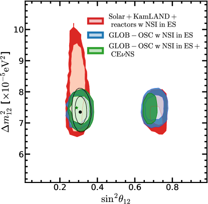
Figure 7: Two-dimensional projections of the allowed regions (at 90% and $3\sigma$ CL) onto $\Delta m^{2}_{12}$ and $\theta_{12}$ parameters, after marginalizing over all other oscillation parameters and over NSI couplings to quarks and electrons. Red regions correspond to the analysis of KamLAND and Solar data; blue regions include all oscillation data; and green regions include all oscillation and CE$\nu$NS data. In all cases, NSI effects on ES are fully accounted for in the fit. For comparison, the empty contours (solid black lines) show the corresponding regions for the global oscillation analysis without NSI.

3.5 Present status of the LMA-D solution

In this section, we discuss in more detail the present status of the LMA-D region in light of all available data, for models leading to NSI couplings to quarks and electrons simultaneously. We start by exploring the dependence of the presence of the LMA-D solution on the specific combination of couplings to the charged fermions considered. In order to do so it is convenient to introduce the functions $\chi^{2}_{\text{LMA}}(\eta,\zeta)$ and $\chi^{2}_{\text{LMA-D}}(\eta,\zeta)$ which are obtained by marginalizing the $\chi^{2}$ for a given value of $\eta$ and $\zeta$ over both the oscillation and the matter potential parameters within the regions $\theta_{12}<45^{\circ}$ and $\theta_{12}>45^{\circ}$, respectively. With this, in the left (central) panels of Fig. 8 we plot isocontours of the differences $\chi^{2}_{\text{LMA}}(\eta,\zeta)-\chi^{2}_{\text{no-NSI}}$ ($\chi^{2}_{\text{LMA-D}}(\eta,\zeta)-\chi^{2}_{\text{no-NSI}}$) where $\chi^{2}_{\text{no-NSI}}$ is the minimum $\chi^{2}$ for standard $3\nu$ oscillations (i.e., without NSI). In the right panels we plot $\chi^{2}_{\text{LMA-D}}(\eta,\zeta)-\chi^{2}_{\text{LMA}}(\eta,\zeta)$ which quantifies the relative quality of the LMA and LMA-D solutions. In each row in this figure we include only a subset of the data as indicated by the labels.

The upper panels of Fig. 8 show the results when only oscillation data is analyzed accounting for the effects of NSI on the matter potential, but without including the effect of NSI in the ES cross sections in Borexino, SNO, and SK. As outlined in Sec. 3.1, these results would therefore apply to NSI models with very light mediators, $M_{\text{med}}\ll 500~{}\text{keV}$. In this scenario (as shown in Sec. 2.1) only the combination of NSI couplings to electrons, protons and neutrons, parametrized by the effective angle $\eta^{\prime}$ in Eq. (19), is relevant. Therefore the $\Delta\chi^{2}$ isocontours are curves along $\tan\eta^{\prime}=\tan\eta\mathbin{/}(\cos\zeta+\sin\zeta)=\text{constant}$. From the upper left panel we see that for most of $(\eta,\zeta)$ values, the inclusion of NSI leads only to a mild improvement of the global fit to oscillation data ($\chi^{2}_{\text{LMA}}(\eta,\zeta)-\chi^{2}_{\text{no-NSI}}>-4$). As discussed in Ref. Esteban:2018ppq (Addendum), with the updated SK4 solar data the determination of $\Delta m^{2}_{21}$ in solar and in KamLAND experiments are fully compatible at $\lesssim 2\sigma$ level. The inclusion of NSI only leads to an overall better fit at a CL above 2$\sigma$ (but still not statistically significant in any of the different data samples) for $(\zeta,\eta)$ along the darker band. In particular the best fit lies along $\tan\eta^{\prime}\sim-1\big{/}Y_{n}^{\oplus}\approx-0.95$ ($\eta^{\prime}\approx-43.6^{\circ}$) for which NSI effects in the Earth matter cancel, so there is no constraint from Atmospheric and LBL experiments on the NSI which can lead to that slightly better fit to Solar + KamLAND data within the LMA solution. The central and right panels show the status of the LMA-D solution in this scenario. We find that LMA-D provides a good solution in most of the $(\eta,\zeta)$ plane. The LMA-D is only very disfavoured for $(\zeta,\eta)$ along the band with $\-2.75\lesssim\tan\eta^{\prime}\lesssim-1.75$. For these values the NSI contribution to the matter potential in the Sun cancels in some point inside the neutrino production area and therefore the degeneracy between NSI and the octant of $\theta_{12}$ cannot be realized.

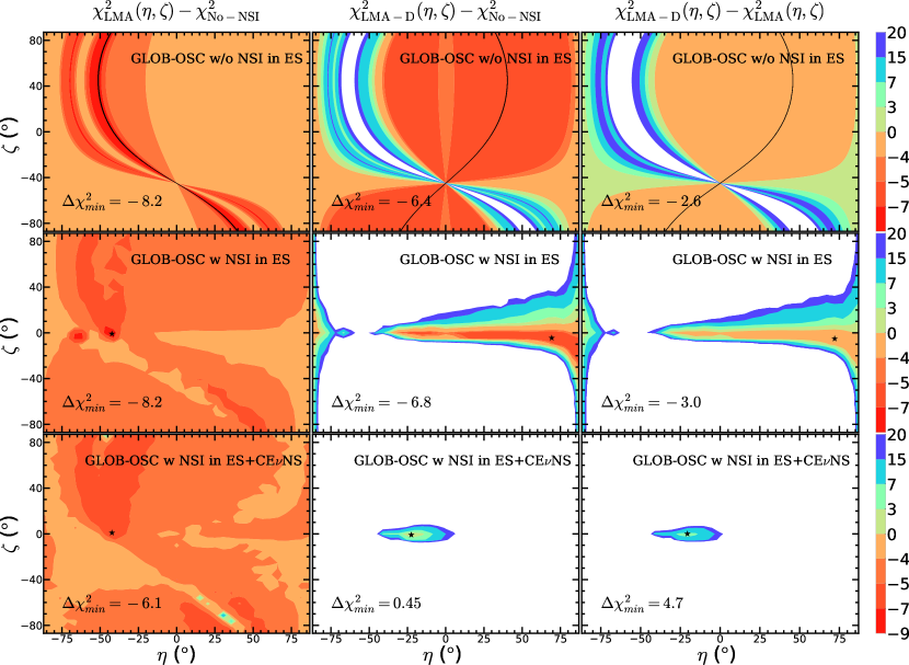
Figure 8: Isocontours of $\chi^{2}_{\text{LMA}}(\eta,\zeta)-\chi^{2}_{\text{no-NSI}}$, $\chi^{2}_{\text{LMA-D}}(\eta,\zeta)-\chi^{2}_{\text{no-NSI}}$ and $\chi^{2}_{\text{LMA-D}}(\eta,\zeta)-\chi^{2}_{\text{LMA-D}}(\eta,\zeta)$ of the global analysis of oscillation data without including NSI in the ES cross sections at Borexino, SNO, and SK (upper panels), and including the NSI in the ES cross sections at Borexino, SNO, and SK (middle panels). The lower panels shows of the result adding the data from CE$\nu$NS experiments. We show projections in the plane of angles ($\zeta$, $\eta$) (after marginalization of all other parameters) which parametrize the relative strength of the NSI couplings to up-quarks, down-quark, and electrons. The levels corresponding to the different colours are given on the color bar on the right. Contours beyond 20 are white. In each panel the best-fit point is marked with a star (middle and bottom rows) or by a solid black line (upper row). Results in the upper row are applicable to NSI induced by mediators with $M_{\text{med}}\ll 500~{}\text{keV}$; in the middle row, for models with $M_{\text{med}}\gtrsim 10~{}\text{MeV}$; and in the lower row, for models with $M_{\text{med}}\gtrsim 50~{}\text{MeV}$, see Sec. 3.1 for details.

The impact of including NSI in the ES cross section in Borexino, SNO, and SK can be seen in the middle row panels in Fig. 8. Since these panels include the effect of NSI in ES, they apply to NSI models with mediator masses $10~{}\text{MeV}\lesssim M_{\text{med}}\lesssim 50~{}\text{MeV}$. The main effect is that the $\zeta$ values for which the LMA-D solution is allowed become very restricted (in fact the best fit point for all panels are always close to $\zeta=0$) as long as $\eta$ does not approach $90^{\circ}$, and consequently the dependence of $\zeta$ is heavily suppressed. Thus, once the effect of NSI in the ES cross section is included, the results are not very different from those obtained for $\zeta=0$ (no coupling to electrons) in Refs. Esteban:2018ppq ; Coloma:2019mbs . The middle and right panels in this row also illustrate how, as long as only oscillation data is included, the LMA-D solution is still allowed with a CL comparable and even slightly better than LMA.

The lower panels in Fig. 8 include the combination of all data available and are therefore applicable to NSI with mediators above $M_{\text{med}}\gtrsim 50~{}\text{MeV}$. When comparing the LMA (LMA-D) to the SM hypothesis (i.e., no NSI) we find that the global minimum of the fit is better (comparable) to that obtained in absence of NSI, as shown in the middle and left panels. However, we also see that the inclusion of the CE$\nu$NS data in the analysis severely constrains the LMA-D solution. Quantitatively we find that LMA-D becomes disfavoured with respect to LMA with $\Delta\chi^{2}>4.7$ for any value of $(\eta,\zeta)$ (right panel) and it is only allowed below $\Delta\chi^{2}=9$ for very specific combinations of couplings to quarks and electrons, $-2.5^{\circ}\leq\zeta\leq 1.5^{\circ}$ and $-29^{\circ}\leq\eta\leq-13^{\circ}$.

To further illustrate the role of the different experiments in this conclusion we show in Fig. 9 the projection of $\chi^{2}_{\text{LMA-D}}(\eta,\zeta)-\chi^{2}_{\text{LMA}}(\eta,\zeta)$ on $\eta$ after marginalizing over $\zeta$ (which, as discussed above, it is effectively not very different from fixing $\zeta=0$). The figure illustrates the complementarity of the CE$\nu$NS data with different targets. As discussed in Sec. 2.2.3, the effects of NSI in CE$\nu$NS on a given target, characterized by a value of $Y_{n}$, cancel for $\eta^{\prime\prime}=\arctan(-1/Y_{n})$ (with $\tan\eta^{\prime\prime}=\tan\eta/\cos\zeta\simeq\tan\eta$). This corresponds to $\eta\simeq-35.4^{\circ}$ ($Y_{n}^{\text{CsI}}\approx 1.407$), $-39.3^{\circ}$ ($Y_{n}^{\text{Ar}}\approx 1.222$), and $-38.4^{\circ}$ ($Y_{n}^{\text{Ge}}\approx 1.263$) for CsI, Ar, and Ge respectively. Thus, as seen in the figure, the combination of the constraints from CE$\nu$NS with the different targets is important to disfavour the LMA-D solution.

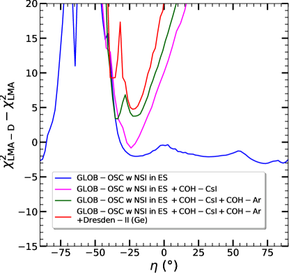
Figure 9: Dependence of $\chi^{2}_{\text{LMA-D}}(\eta,\zeta)-\chi^{2}_{\text{LMA}}(\eta,\zeta)$ on $\eta$ after marginalizing over $\zeta$ for different combination of experiments as labeled in the figure.

4 Summary

In this work we have presented an updated analysis of neutrino oscillation data and in combination with the results of CE$\nu$NS on a variety of targets with the aim of establishing the allowed size and flavour structure of CP-conserving NC NSI which affect either the evolution of neutrinos in a matter background and/or their detection cross section. We have included in our fit all the latest solar, atmospheric, reactor and accelerator data used for the standard 3$\nu$ oscillation analysis in NuFIT-5.2 with the only exception of T2K and NO$\nu$A appearance data whose hints in of CP violation cannot be accommodated within the CP-conserving approximation assumed in this work. When combining with CE$\nu$NS we include the results from COHERENT data on CSI and Ar detectors, together with the results Dresden-II reactor experiment with a Ge detector.

The study extends previous works by considering either vector or axial NSI with an arbitrary ratio of couplings to up-quarks, down-quarks, and electrons (parametrized by two angles, $\eta$ and $\zeta$). In the oscillation analysis including vector NSI involving interactions with electrons ($\zeta\neq 0$), which could affect both the propagation and ES detection cross section in Borexino, SNO, and SK, we have consistently accounted for the interplay of flavour transitions in both effects by employing the density matrix formalism (which we had previously proposed). Furthermore we have considered two scenarios: (a) including the NSI only in the matter effects (characteristic of models where NSI are generated by mediators much lighter than $\mathcal{O}(500~{}\text{keV})$), and (b) including the NSI both in propagation, CE$\nu$NS, and ES scattering (characteristic of models where NSI are generated by mediators heavier than $\mathcal{O}(50~{}\text{MeV})$). Our results show that:

• From the methodological point of view, the validity of the adiabaticity assumption for the neutrino propagation in the Sun in the presence of NSI (and of NP, in general) is not a given. But we conclude that using the adiabatic approximation leads to the correct allowed ranges of NSI coefficients in all cases studied, as long as one removes from the explored space of NSI couplings those points for which adiabaticity in the Sun is violated.

• The global oscillation analysis of vector NSI which enter only via the matter potential leads to the bounds on the five combinations $\varepsilon_{ee}^{f,V}-\varepsilon_{\mu\mu}^{f,V}$ and $\varepsilon_{\tau\tau}^{f,V}-\varepsilon_{\mu\mu}^{f,V}$ and $\varepsilon^{f,V}_{\alpha\neq\beta}$ shown in Fig. 2 and Table 1 for interactions with electrons, and in the first column in Table 3 for interactions with up and down quark. The 90% bounds range from $\sim 0.5$% to $\sim 30$% for $\varepsilon_{\tau\tau}^{f,V}-\varepsilon_{\mu\mu}^{f,V}$ and $\varepsilon^{f,V}_{\alpha\neq\beta}$, while $\varepsilon_{ee}^{f,V}-\varepsilon_{\mu\mu}^{f,V}$ presents two (quasi)degenerate allowed ranges around $0$ and $\sim-2$ ($\sim-1$) for NSI with electrons (quarks) which correspond to the well-known LMA and LMA-D solutions.

• The LMA-D solution is realized for generic vector NSI couplings to electrons and quarks as long as only considering propagation effects (see first row in Fig. 8) unless the couplings come in a ratio that cancels their contribution to the solar matter potential ($\-2.75\lesssim\tan\eta\mathbin{/}(\cos\zeta+\sin\zeta)\lesssim-1.75$).

• Including the effect of the vector NSI in the ES scattering cross sections in Borexino, SK and SNO, lifts the degeneracy and disfavours the LMA-D solution unless the NSI coupling to the electrons is suppressed compared to the coupling to quarks (see second row in Fig. 8). But it still provides a good fit to the data for a wide range of ratios of the couplings to up and down quarks, and it is allowed at 3$\sigma$ for $\eta<-70^{\circ}$ or $\eta>-40^{\circ}$ (see Fig. 9).

• For vector NSI coupling to electrons only, the inclusion of NSI in the ES scattering cross sections eliminates the LMA-D solution and allows for independent determination of the three $\varepsilon_{\alpha\alpha}^{f,V}$. But within the LMA solution, our comparative results show that it is the presence of the NSI in the matter potential which drives the strong constraints.

• For vector NSI coupling mostly to quarks induced by mediators with $M_{\text{med}}\gtrsim 50~{}\text{MeV}$, the combination of the oscillation results with the data from CE$\nu$NS disfavours the LMA-D solution beyond $\sim 2\sigma$ for any value of $\eta$ and it is only allowed below $\Delta\chi^{2}=9$ for $-29^{\circ}\leq\eta\leq-13$. (see Figs. 8 and 9). We find that the combination of CE$\nu$NS with different nuclear targets is important to disfavour the LMA-D solution at that level.

• The determination of the oscillation parameters within the LMA region is rather robust even after the inclusion of NSI couplings to both quarks and electrons as large as allowed by the global oscillation data analysis itself (see Fig. 7).

• Axial-vector NSI only enter in the analysis via their effects in the interaction of solar neutrinos in Borexino, SNO, and SK when coupling to electrons, or in the NC rate in SNO when coupling to quarks. For interactions with electrons their bounds are notably weaker than those on vector NSI (see Fig. 4 and Table 2). For interactions with quarks they cannot be all independently bounded (see Table 4 for one parameter bounds).

Moreover, to quantify the possible implications that generic models leading to NSI may have for future Earth-based facilities, we have projected the results of our analysis in terms of the effective NSI parameters which describe the generalized matter potential in the Earth, relevant for the study of atmospheric and long-baseline neutrino oscillation experiments (see Fig. 6 and Table 5).

To summarize, this work provides the most general study of NSI involving quarks and electrons up to date using neutrino oscillation data and measurements of CE$\nu$NS using neutrinos from spallation and reactor sources. While the scope of this work is restricted to neutrino facilities, dark matter direct detection experiments are rapidly approaching the so-called neutrino floor. If affected by NSI, significant deviations on the expected results may be observable Cerdeno:2016sfi ; Boehm:2018sux ; Gonzalez-Garcia:2018dep . While present experiments are not competitive yet in this regard, the upcoming generation of experiments will soon provide interesting limits on NSI and may offer additional synergies with neutrino oscillation and CE$\nu$NS data Amaral:2023tbs .

- (1) B. Pontecorvo, Neutrino Experiments and the Problem of Conservation of Leptonic Charge, Sov. Phys. JETP 26 (1968) 984. [Zh. Eksp. Teor. Fiz.53,1717(1967)].
- (2) V.N. Gribov and B. Pontecorvo, Neutrino astronomy and lepton charge, Phys. Lett. B28 (1969) 493.
- (3) M.C. Gonzalez-Garcia and M. Maltoni, Phenomenology with Massive Neutrinos, Phys. Rept. 460 (2008) 1 [0704.1800].
- (4) A. Falkowski, M. González-Alonso, J. Kopp, Y. Soreq and Z. Tabrizi, EFT at FASER, JHEP 10 (2021) 086 [2105.12136].
- (5) V. Bresó-Pla, A. Falkowski, M. González-Alonso and K. Monsálvez-Pozo, EFT analysis of New Physics at COHERENT, 2301.07036.
- (6) A. Falkowski, M. González-Alonso and Z. Tabrizi, Consistent QFT description of non-standard neutrino interactions, JHEP 11 (2020) 048 [1910.02971].
- (7) A. Falkowski, M. González-Alonso and Z. Tabrizi, Reactor neutrino oscillations as constraints on Effective Field Theory, JHEP 05 (2019) 173 [1901.04553].
- (8) S. Davidson, C. Pena-Garay, N. Rius and A. Santamaria, Present and future bounds on nonstandard neutrino interactions, JHEP 03 (2003) 011 [hep-ph/0302093].
- (9) C. Biggio, M. Blennow and E. Fernandez-Martinez, General bounds on non-standard neutrino interactions, JHEP 08 (2009) 090 [0907.0097].
- (10) C. Biggio, M. Blennow and E. Fernandez-Martinez, Loop bounds on non-standard neutrino interactions, JHEP 03 (2009) 139 [0902.0607].
- (11) M.B. Gavela, D. Hernandez, T. Ota and W. Winter, Large gauge invariant non-standard neutrino interactions, Phys. Rev. D79 (2009) 013007 [0809.3451].
- (12) S. Antusch, J.P. Baumann and E. Fernandez-Martinez, Non-Standard Neutrino Interactions with Matter from Physics Beyond the Standard Model, Nucl. Phys. B810 (2009) 369 [0807.1003].
- (13) P.S. Bhupal Dev et al., Neutrino Non-Standard Interactions: A Status Report, in NTN Workshop on Neutrino Non-Standard Interactions St Louis, MO, USA, May 29-31, 2019, 2019, http://lss.fnal.gov/archive/2019/conf/fermilab-conf-19-299-t.pdf [1907.00991].
- (14) K.S. Babu, A. Friedland, P.A.N. Machado and I. Mocioiu, Flavor Gauge Models Below the Fermi Scale, JHEP 12 (2017) 096 [1705.01822].
- (15) Y. Farzan, A model for large non-standard interactions of neutrinos leading to the LMA-Dark solution, Phys. Lett. B 748 (2015) 311 [1505.06906].
- (16) Y. Farzan and J. Heeck, Neutrinophilic nonstandard interactions, Phys. Rev. D 94 (2016) 053010 [1607.07616].
- (17) Y. Farzan and I.M. Shoemaker, Lepton Flavor Violating Non-Standard Interactions via Light Mediators, JHEP 07 (2016) 033 [1512.09147].
- (18) A. Greljo, P. Stangl, A.E. Thomsen and J. Zupan, On (g 2)μ from gauged U(1)X, JHEP 07 (2022) 098 [2203.13731].
- (19) J. Heeck, M. Lindner, W. Rodejohann and S. Vogl, Non-Standard Neutrino Interactions and Neutral Gauge Bosons, SciPost Phys. 6 (2019) 038 [1812.04067].
- (20) Y. Farzan, A model for lepton flavor violating non-standard neutrino interactions, Phys. Lett. B 803 (2020) 135349 [1912.09408].
- (21) N. Bernal and Y. Farzan, Neutrino nonstandard interactions with arbitrary couplings to u and d quarks, Phys. Rev. D 107 (2023) 035007 [2211.15686].
- (22) K.S. Babu, P.S.B. Dev, S. Jana and A. Thapa, Non-Standard Interactions in Radiative Neutrino Mass Models, JHEP 03 (2020) 006 [1907.09498].
- (23) M.B. Wise and Y. Zhang, Effective Theory and Simple Completions for Neutrino Interactions, Phys. Rev. D 90 (2014) 053005 [1404.4663].
- (24) A. Greljo, Y. Soreq, P. Stangl, A.E. Thomsen and J. Zupan, Muonic force behind flavor anomalies, JHEP 04 (2022) 151 [2107.07518].
- (25) P. Coloma, M.C. Gonzalez-Garcia and M. Maltoni, Neutrino oscillation constraints on U(1)’ models: from non-standard interactions to long-range forces, JHEP 01 (2021) 114 [2009.14220]. [Erratum: JHEP 11, 115 (2022)].
- (26) L. Wolfenstein, Neutrino Oscillations in Matter, Phys. Rev. D17 (1978) 2369.
- (27) S.P. Mikheev and A.Y. Smirnov, Resonance enhancement of oscillations in matter and solar neutrino spectroscopy, Sov. J. Nucl. Phys. 42 (1985) 913.
- (28) M.C. Gonzalez-Garcia and M. Maltoni, Determination of matter potential from global analysis of neutrino oscillation data, JHEP 09 (2013) 152 [1307.3092].
- (29) I. Esteban, M.C. Gonzalez-Garcia, M. Maltoni, I. Martinez-Soler and J. Salvado, Updated constraints on non-standard interactions from global analysis of oscillation data, JHEP 08 (2018) 180 [1805.04530]. [Addendum: JHEP 12, 152 (2020)].
- (30) J.W.F. Valle, Resonant Oscillations of Massless Neutrinos in Matter, Phys. Lett. B199 (1987) 432.
- (31) M.M. Guzzo, A. Masiero and S.T. Petcov, On the MSW effect with massless neutrinos and no mixing in the vacuum, Phys. Lett. B260 (1991) 154.
- (32) O.G. Miranda, M.A. Tortola and J.W.F. Valle, Are solar neutrino oscillations robust?, JHEP 10 (2006) 008 [hep-ph/0406280].
- (33) M.C. Gonzalez-Garcia, M. Maltoni and J. Salvado, Testing matter effects in propagation of atmospheric and long-baseline neutrinos, JHEP 05 (2011) 075 [1103.4365].
- (34) P. Bakhti and Y. Farzan, Shedding light on LMA-Dark solar neutrino solution by medium baseline reactor experiments: JUNO and RENO-50, JHEP 07 (2014) 064 [1403.0744].
- (35) P. Coloma and T. Schwetz, Generalized mass ordering degeneracy in neutrino oscillation experiments, Phys. Rev. D94 (2016) 055005 [1604.05772].
- (36) K. Scholberg, Prospects for measuring coherent neutrino-nucleus elastic scattering at a stopped-pion neutrino source, Phys. Rev. D 73 (2006) 033005 [hep-ex/0511042].
- (37) J. Barranco, O.G. Miranda, C.A. Moura and J.W.F. Valle, Constraining non-standard interactions in nu(e) e or anti-nu(e) e scattering, Phys. Rev. D 73 (2006) 113001 [hep-ph/0512195].
- (38) J. Barranco, O.G. Miranda and T.I. Rashba, Probing New Physics with Coherent Neutrino Scattering Off Nuclei, JHEP 12 (2005) 021 [hep-ph/0508299].
- (39) J. Barranco, O.G. Miranda, C.A. Moura and J.W.F. Valle, Constraining non-standard neutrino-electron interactions, Phys. Rev. D 77 (2008) 093014 [0711.0698].
- (40) A. Bolanos, O.G. Miranda, A. Palazzo, M.A. Tortola and J.W.F. Valle, Probing non-standard neutrino-electron interactions with solar and reactor neutrinos, Phys. Rev. D 79 (2009) 113012 [0812.4417].
- (41) F.J. Escrihuela, O.G. Miranda, M.A. Tortola and J.W.F. Valle, Constraining nonstandard neutrino-quark interactions with solar, reactor and accelerator data, Phys. Rev. D80 (2009) 105009 [0907.2630]. [Erratum: Phys. Rev.D80,129908(2009)].
- (42) D.Z. Freedman, Coherent Neutrino Nucleus Scattering as a Probe of the Weak Neutral Current, Phys. Rev. D9 (1974) 1389.
- (43) P. Coloma, P.B. Denton, M.C. Gonzalez-Garcia, M. Maltoni and T. Schwetz, Curtailing the Dark Side in Non-Standard Neutrino Interactions, JHEP 04 (2017) 116 [1701.04828].
- (44) I.M. Shoemaker, COHERENT search strategy for beyond standard model neutrino interactions, Phys. Rev. D 95 (2017) 115028 [1703.05774].
- (45) P. Coloma, M.C. Gonzalez-Garcia, M. Maltoni and T. Schwetz, COHERENT enlightenment of the neutrino dark side, Phys. Rev. D96 (2017) 115007 [1708.02899].
- (46) COHERENT collaboration, Observation of Coherent Elastic Neutrino-Nucleus Scattering, Science 357 (2017) 1123 [1708.01294].
- (47) P. Coloma, I. Esteban, M.C. Gonzalez-Garcia and M. Maltoni, Improved global fit to Non-Standard neutrino Interactions using COHERENT energy and timing data, JHEP 02 (2020) 023 [1911.09109]. [Addendum: JHEP 12, 071 (2020)].
- (48) COHERENT collaboration, COHERENT Collaboration data release from the first observation of coherent elastic neutrino-nucleus scattering, 1804.09459.
- (49) COHERENT collaboration, First Measurement of Coherent Elastic Neutrino-Nucleus Scattering on Argon, Phys. Rev. Lett. 126 (2021) 012002 [2003.10630].
- (50) J. Colaresi, J.I. Collar, T.W. Hossbach, A.R.L. Kavner, C.M. Lewis, A.E. Robinson et al., First results from a search for coherent elastic neutrino-nucleus scattering at a reactor site, Phys. Rev. D 104 (2021) 072003 [2108.02880].
- (51) M. Chaves and T. Schwetz, Resolving the LMA-dark NSI degeneracy with coherent neutrino-nucleus scattering, JHEP 05 (2021) 042 [2102.11981].
- (52) P. Coloma, I. Esteban, M.C. Gonzalez-Garcia, L. Larizgoitia, F. Monrabal and S. Palomares-Ruiz, Bounds on new physics with data of the Dresden-II reactor experiment and COHERENT, 2202.10829.
- (53) Borexino collaboration, Constraints on flavor-diagonal non-standard neutrino interactions from Borexino Phase-II, JHEP 02 (2020) 038 [1905.03512].
- (54) P. Coloma, P. Coloma, M.C. Gonzalez-Garcia, M.C. Gonzalez-Garcia, M. Maltoni, M. Maltoni et al., Constraining new physics with Borexino Phase-II spectral data, JHEP 07 (2022) 138 [2204.03011]. [Erratum: JHEP 11, 138 (2022)].
- (55) COHERENT collaboration, COHERENT Collaboration data release from the first detection of coherent elastic neutrino-nucleus scattering on Argon, 2006.12659.
- (56) J. Colaresi, J.I. Collar, T.W. Hossbach, C.M. Lewis and K.M. Yocum, Suggestive evidence for Coherent Elastic Neutrino-Nucleus Scattering from reactor antineutrinos, 2202.09672.
- (57) D.W.P. Amaral, D. Cerdeno, A. Cheek and P. Foldenauer, A direct detection view of the neutrino NSI landscape, 2302.12846.
- (58) Z. Maki, M. Nakagawa and S. Sakata, Remarks on the unified model of elementary particles, Prog. Theor. Phys. 28 (1962) 870.
- (59) M. Kobayashi and T. Maskawa, CP Violation in the Renormalizable Theory of Weak Interaction, Prog. Theor. Phys. 49 (1973) 652.
- (60) I. Esteban, M.C. Gonzalez-Garcia, M. Maltoni, I. Martinez-Soler and T. Schwetz, Updated fit to three neutrino mixing: exploring the accelerator-reactor complementarity, 1611.01514.
- (61) A. Dziewonski and D. Anderson, Preliminary reference earth model, Phys.Earth Planet.Interiors 25 (1981) 297.
- (62) A. Friedland, C. Lunardini and M. Maltoni, Atmospheric neutrinos as probes of neutrino-matter interactions, Phys.Rev. D70 (2004) 111301 [hep-ph/0408264].
- (63) J.N. Bahcall, M. Kamionkowski and A. Sirlin, Solar neutrinos: Radiative corrections in neutrino - electron scattering experiments, Phys. Rev. D 51 (1995) 6146 [astro-ph/9502003].
- (64) J.N. Bahcall, K. Kubodera and S. Nozawa, Neutral Current Reactions of Solar and Supernova Neutrinos on Deuterium, Phys. Rev. D 38 (1988) 1030.
- (65) J. Bernabeu, T.E.O. Ericson, E. Hernandez and J. Ros, Effects of the axial isoscalar neutral current for solar neutrino detection, Nucl. Phys. B 378 (1992) 131.
- (66) J.-W. Chen, K.M. Heeger and R.G.H. Robertson, Constraining the leading weak axial two-body current by SNO and super-K, Phys. Rev. C 67 (2003) 025801 [nucl-th/0210073].
- (67) I. Esteban, M.C. Gonzalez-Garcia, M. Maltoni, T. Schwetz and A. Zhou, “NuFIT 5.2 (2022).” http://www.nu-fit.org.
- (68) B.T. Cleveland et al., Measurement of the solar electron neutrino flux with the Homestake chlorine detector, Astrophys. J. 496 (1998) 505.
- (69) F. Kaether, W. Hampel, G. Heusser, J. Kiko and T. Kirsten, Reanalysis of the GALLEX solar neutrino flux and source experiments, Phys. Lett. B685 (2010) 47 [1001.2731].
- (70) SAGE collaboration, Measurement of the solar neutrino capture rate with gallium metal. III: Results for the 2002--2007 data-taking period, Phys. Rev. C80 (2009) 015807 [0901.2200].
- (71) Super-Kamiokande collaboration, Solar neutrino measurements in Super-Kamiokande-I, Phys. Rev. D73 (2006) 112001 [hep-ex/0508053].
- (72) Super-Kamiokande collaboration, Solar neutrino measurements in Super-Kamiokande-II, Phys. Rev. D78 (2008) 032002 [0803.4312].
- (73) Super-Kamiokande collaboration, Solar neutrino results in Super-Kamiokande-III, Phys. Rev. D83 (2011) 052010 [1010.0118].
- (74) Y. Nakajima, ‘‘Recent results and future prospects from Super-Kamiokande.’’ Talk given at the XXIX International Conference on Neutrino Physics and Astrophysics, Chicago, USA, June 22--July 2, 2020 (online conference).
- (75) SNO collaboration, Measurement of the nu/e and total B-8 solar neutrino fluxes with the Sudbury Neutrino Observatory phase I data set, Phys. Rev. C75 (2007) 045502 [nucl-ex/0610020].
- (76) SNO collaboration, Electron energy spectra, fluxes, and day-night asymmetries of B-8 solar neutrinos from the 391-day salt phase SNO data set, Phys. Rev. C72 (2005) 055502 [nucl-ex/0502021].
- (77) SNO collaboration, An Independent Measurement of the Total Active 8B Solar Neutrino Flux Using an Array of 3He Proportional Counters at the Sudbury Neutrino Observatory, Phys. Rev. Lett. 101 (2008) 111301 [0806.0989].
- (78) SNO collaboration, Combined Analysis of all Three Phases of Solar Neutrino Data from the Sudbury Neutrino Observatory, 1109.0763.
- (79) Borexino collaboration, Precision measurement of the 7Be solar neutrino interaction rate in Borexino, Phys. Rev. Lett. 107 (2011) 141302 [1104.1816].
- (80) Borexino collaboration, Measurement of the solar 8B neutrino rate with a liquid scintillator target and 3 MeV energy threshold in the Borexino detector, Phys. Rev. D82 (2010) 033006 [0808.2868].
- (81) Borexino collaboration, First Simultaneous Precision Spectroscopy of , 7Be, and Solar Neutrinos with Borexino Phase-II, Phys. Rev. D 100 (2019) 082004 [1707.09279].
- (82) KamLAND collaboration, Reactor On-Off Antineutrino Measurement with KamLAND, Phys. Rev. D88 (2013) 033001 [1303.4667].
- (83) Daya Bay collaboration, Improved Measurement of the Reactor Antineutrino Flux and Spectrum at Daya Bay, Chin. Phys. C41 (2017) 013002 [1607.05378].
- (84) T. Bezerra, ‘‘New Results from the Double Chooz Experiment.’’ Talk given at the XXIX International Conference on Neutrino Physics and Astrophysics, Chicago, USA, June 22--July 2, 2020 (online conference).
- (85) Daya Bay collaboration, Precision measurement of reactor antineutrino oscillation at kilometer-scale baselines by Daya Bay, 2211.14988.
- (86) J. Yoo, ‘‘RENO.’’ Talk given at the XXIX International Conference on Neutrino Physics and Astrophysics, Chicago, USA, June 22--July 2, 2020 (online conference).
- (87) Super-Kamiokande collaboration, Atmospheric Results from Super-Kamiokande, AIP Conf. Proc. 1666 (2015) 100001 [1412.5234]. slides available at https://indico.fnal.gov/event/8022/other-view?view=standard.
- (88) IceCube collaboration, Determining neutrino oscillation parameters from atmospheric muon neutrino disappearance with three years of IceCube DeepCore data, Phys. Rev. D91 (2015) 072004 [1410.7227].
- (89) IceCube collaboration, ‘‘IceCube Oscillations: 3 years muon neutrino disappearance data.’’ http://icecube.wisc.edu/science/data/nu_osc.
- (90) IceCube collaboration, Searches for Sterile Neutrinos with the IceCube Detector, Phys. Rev. Lett. 117 (2016) 071801 [1605.01990].
- (91) MINOS collaboration, Measurement of Neutrino and Antineutrino Oscillations Using Beam and Atmospheric Data in MINOS, Phys. Rev. Lett. 110 (2013) 251801 [1304.6335].
- (92) P. Dunne, ‘‘Latest Neutrino Oscillation Results from T2K.’’ Talk given at the XXIX International Conference on Neutrino Physics and Astrophysics, Chicago, USA, June 22--July 2, 2020 (online conference).
- (93) A. Himmel, ‘‘New Oscillation Results from the NOvA Experiment.’’ Talk given at the XXIX International Conference on Neutrino Physics and Astrophysics, Chicago, USA, June 22--July 2, 2020 (online conference).
- (94) J.I. Collar, A.R.L. Kavner and C.M. Lewis, Response of CsI[Na] to Nuclear Recoils: Impact on Coherent Elastic Neutrino-Nucleus Scattering (CENS), Phys. Rev. D 100 (2019) 033003 [1907.04828].
- (95) P. Klos, J. Menéndez, D. Gazit and A. Schwenk, Large-scale nuclear structure calculations for spin-dependent WIMP scattering with chiral effective field theory currents, Phys. Rev. D 88 (2013) 083516 [1304.7684]. [Erratum: Phys.Rev.D 89, 029901 (2014)].
- (96) R.H. Helm, Inelastic and Elastic Scattering of 187-Mev Electrons from Selected Even-Even Nuclei, Phys. Rev. 104 (1956) 1466.
- (97) J.I. Collar, A.R.L. Kavner and C.M. Lewis, Germanium response to sub-keV nuclear recoils: a multipronged experimental characterization, Phys. Rev. D 103 (2021) 122003 [2102.10089].
- (98) M.C. Gonzalez-Garcia, P.C. de Holanda, E. Masso and R. Zukanovich Funchal, Probing long-range leptonic forces with solar and reactor neutrinos, JCAP 01 (2007) 005 [hep-ph/0609094].
- (99) F. Feroz, M.P. Hobson, E. Cameron and A.N. Pettitt, Importance Nested Sampling and the MultiNest Algorithm, Open J. Astrophys. 2 (2019) 10 [1306.2144].
- (100) F. Feroz, M.P. Hobson and M. Bridges, MultiNest: an efficient and robust Bayesian inference tool for cosmology and particle physics, Mon. Not. Roy. Astron. Soc. 398 (2009) 1601 [0809.3437].
- (101) GAMBIT collaboration, Comparison of statistical sampling methods with ScannerBit, the GAMBIT scanning module, Eur. Phys. J. C 77 (2017) 761 [1705.07959].
- (102) D.G. Cerdeño, M. Fairbairn, T. Jubb, P.A.N. Machado, A.C. Vincent and C. Bœhm, Physics from solar neutrinos in dark matter direct detection experiments, JHEP 05 (2016) 118 [1604.01025]. [Erratum: JHEP 09, 048 (2016)].
- (103) C. Bœhm, D.G. Cerdeño, P.A.N. Machado, A. Olivares-Del Campo, E. Perdomo and E. Reid, How high is the neutrino floor?, JCAP 01 (2019) 043 [1809.06385].
- (104) M.C. Gonzalez-Garcia, M. Maltoni, Y.F. Perez-Gonzalez and R. Zukanovich Funchal, Neutrino Discovery Limit of Dark Matter Direct Detection Experiments in the Presence of Non-Standard Interactions, JHEP 07 (2018) 019 [1803.03650].