Eight-dimensional topological systems simulated using time-space crystalline structures

Abstract

We demonstrate the possibility of using time-space crystalline structures to simulate eight-dimensional systems based on only two physical dimensions. A suitable choice of system parameters allows us to obtain a gapped energy spectrum, making topological effects become relevant. The nontrivial topology of the system is evinced by considering the adiabatic state pumping along temporal and spatial crystalline directions. Analysis of the system is facilitated by rewriting the system Hamiltonian in a tight-binding form, thereby putting space, time, and the additional synthetic dimensions on an equal footing.

Introduction. Quantum simulation is a rapidly growing and exciting field of study, focused on exploiting controllable quantum systems to replicate and probe complex physical phenomena [1, 2]. Whereas simulating a quantum system with full precision is a daunting task, recreation of specific relevant features is often within reach. In particular, ultracold atomic systems in optical lattices [3] have successfully demonstrated abilities to model intricate condensed-matter and topological phenomena [4, 5] as well as lattice gauge theories [6, 7]. An intriguing line of thought along this direction is the emulation of high-dimensional systems, notably — high-dimensional periodically ordered physical structures — in low-dimensional settings [8, 9, 5, 10, 11, 12]. In this context, several recent proposals drew inspiration from the emergent concept of time crystals [13, 14, 15, 16] and asked if time can play the role of an additional coordinate in quantum simulations. This time-crystalline approach [17, 16] involves a driving signal of a certain frequency to create a repeating pattern of motion at a commensurate frequency that persists over time. Many condensed matter phenomena were thus reenacted in the time domain [16, 18], and the possibility to engage both temporal and spatial dimensions at the same time was established [19, 20, 11, 21], thus doubling the number of available dimensions.

In this Letter, we provide a route for studying topological eight-dimensional (8D) systems that can be experimentally realized using only two physical spatial dimensions. We start with a periodically driven 1D optical lattice with steep barriers (modeled by delta-functions) and show that it can sustain a 2D time-space lattice. The topological nature of the attained time-space crystalline structure is made evident by considering adiabatic state pumping along temporal and spatial crystalline directions. Interpreting the two adiabatic phases as crystal momenta of simulated extra dimensions, we show that the energy bands of the system are characterized by nonvanishing second Chern numbers of the effective 4D lattice. Finally, we demonstrate that two such 4D systems can be combined, and the resulting energy spectrum will remain gapped. The topological properties of the attained 8D system are then characterized by the fourth Chern number, and energy bands with nonvanishing values of the fourth Chern number are identified.

Model. We introduce a 1D time-dependent Hamiltonian

$$\hat{H}(x,\hat{p}_{x},t|\varphi_{x},\varphi_{t})=\hat{h}(x,\hat{p}_{x}|\varphi_{x})+\xi(x,t|\varphi_{t}),$$ (1)

written as a sum of an adiabatic-pumping part $\hat{h}$ (which is static but depends on a spatial adiabatic phase $\varphi_{x}$) and a time-periodic driving term featuring a second adiabatic phase $\varphi_{t}$. Throughout this work, we use the recoil units for the energy $\hbar^{2}k_{{\rm L}}^{2}/2m$ and length $1/k_{{\rm L}}$, with $k_{{\rm L}}$ being the wave number of the primary laser beam used to create the optical lattice and $m$ the particle mass. The unit of time is $\hbar$ divided by the energy unit. The first term of Eq. (1) is the unperturbed spatial Hamiltonian,

$$\hat{h}=\hat{p}_{x}^{2}+V\sum_{n=0}^{3N}\delta(x-\tfrac{na}{3})+U\sum_{n=1}^{3}g_{n}(x)\cos\!\left[\varphi_{x}+\tfrac{2\pi(n-1)}{3}\right].$$ (2)

Here, $\hat{p}_{x}$ is the momentum operator, while the sums describe the spatial potential — a lattice of $N$ identical cells of length $a$, each consisting of three sites separated by steep delta-function barriers, see Fig. 1. The superlattice potential $g_{n}(x)$ is equal to unity only in the $n$th site of each spatial cell and vanishes otherwise. This term modulates the onsite energies in the same way in each cell by changing $\varphi_{x}$, with $U$ controlling the modulation amplitude. Note that the modulation phase in each consecutive site is lagging with respect to its neighbor on the left by one third of a cycle. If the modulation is performed adiabatically, the Thouless pumping can be realized in the system described by $\hat{h}$. The realization of sharp optical barriers as well as three-site Thouless pumping have already been studied in the literature [22, 23, 24].

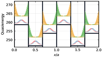
Figure 1: Wannier function densities $|w_{\ell}(x,t=7\pi/4\Omega)|^{2}$ at $\varphi_{x}=\pi/5$, $\varphi_{t}=0$, where $2\pi/\Omega$ is the period of time evolution of $w_{\ell}(x,t)$. The baseline of each Wannier function is shifted upwards along the quasienergy axis by the mean value of quasienergy in the corresponding state, i.e. the quantity $\left\langle w_{\ell}\right|\hat{{\cal H}}\left|w_{\ell}\right\rangle$. At the chosen value of $\varphi_{x}$, each Wannier function is localized almost entirely within a single site, therefore, the infinitesimal “tails” of the functions are not shown. Black vertical lines represent the steep barriers separating the sites of the spatial lattice, while the horizontal lines depict the values of the onsite energies described by the third term in Eq. (2). Parameters of the model are: $N=2$, $s=2$, $a=4.000$, $V=2000$, $U=7.000$, $\omega=676.8$, $\lambda_{{\rm S}}=10.00$, $\lambda_{{\rm L}}=20.00$. Trailing zeros are within the numerical resolution/accuracy and are significant. The nature of the presented results, however, will not change if all the values are chosen within $\sim 10\%$ of the given ones and then $\omega$ is adjusted accordingly to ensure that the quasienergy spectrum is gapped.

The spatial Hamiltonian is perturbed by the terms

$$\begin{split}\xi(x,t|\varphi_{t})=\ &\lambda_{{\rm S}}\cos(\tfrac{12\pi x}{a})\cos(2\omega t)\\ &+\lambda_{{\rm L}}\cos(\tfrac{6\pi x}{a})\cos(\omega t+\varphi_{t}),\end{split}$$ (3)

where $\lambda_{{\rm S}}$ and $\lambda_{{\rm L}}$ control the overall strength of the perturbation. The spatial frequencies $6\pi/a$ and $12\pi/a$ ensure that all spatial sites are perturbed in the same way. The driving frequency $\omega$ is chosen so that a resonant condition is fulfilled in each spatial site. In the classical description, the resonance means that $\omega$ is very close to an integer multiple of the frequency $\Omega$ of the periodic motion of a particle in a spatial site, i.e., $\omega\approx s\Omega$, where $s$ is integer. In the quantum description, the resonance corresponds to $\omega$ being close to an integer multiple of the gap $\Omega$ between certain bands of the Hamiltonian (2). In the limit $V\rightarrow\infty$ [see Eq. (2)] an independent time-crystalline structure is formed in each spatial site due to the resonant driving. Specifically, in the frame evolving along the resonant trajectory, the resonant dynamics of a particle can be described by $\hat{H}_{{\rm eff}}=\hat{\tilde{p}}_{\tilde{x}}^{2}+\tilde{\lambda}_{{\rm S}}\cos(2s\tilde{x})+\tilde{\lambda}_{{\rm L}}\cos(s\tilde{x}+\varphi_{t})$ where $\tilde{x}\in[0,2\pi)$, see Refs. [11, 21]. For example, for $s=2$, there are two temporal cells, each consisting of two temporal sites. An adiabatic change of the phase $\varphi_{t}$ allows for a realization of the Thouless pumping in the time-crystalline structures [21]. If $V<\infty$, then tunneling of a particle between spatial sites is possible, and the entire system forms a 2D time-space crystalline structure which, as we will show, can be described by a 2D tight-binding model.

To study the emergence of a time-space crystalline structure and the pumping dynamics, we solve the eigenvalue problem $\hat{{\cal H}}u_{n,k}(x,t)=\varepsilon_{n,k}u_{n,k}(x,t)$ for the Floquet Hamiltonian $\hat{{\cal H}}=\hat{H}-\mathrm{i}\partial_{t}$ [25, 26, 27]. We assume periodic boundary conditions for the spatial system and introduce the spatial quasimomentum $k$. We denote the quasienergy of the $n$th eigenstate by $\varepsilon_{n,k}$, while $u_{n,k}(x,t)$ is the corresponding Floquet mode that respects temporal periodicity of the perturbation: $u_{n,k}(x,t)=u_{n,k}(x,t+2\pi/\omega)$. A general solution of the Schr\̈mathrm{i}¿œdinger equation can be represented as a superposition of states $\Psi_{n,k}(x,t)=\mathrm{e}^{-\mathrm{i}\varepsilon_{n,k}t}u_{n,k}(x,t).$ In our simulations we consider a finite number of spatial cells, $N=2$, and a finite number of temporal cells, $s=2$. The considered values of quasimomentum are thus $k=0$ and $k=\pi$ (assuming $k\in[0;2\pi)$), corresponding to the boundary of the Brillouin zone. Consequently, the obtained widths of the energy bands coincide with the widths being approached in the limit $N\to\infty$.

The details of the diagonalization procedure are covered in the Supplemental Material [28]. All calculations have been performed using a number of software packages [29, 30, 31, 32, 33, 34] written in the Julia programming language [35]. The source code of our package is available on GitHub [36].

The resonant subspace of the entire Hilbert space which we are interested in consists of $3N\times 2s$ eigenstates. Diagonalizing the periodic position operator $\mathrm{e}^{\mathrm{i}\frac{2\pi}{Na}x}$ in this subspace [37, 38] we obtain $6Ns$ Wannier functions $w_{\ell}(x,t)$ of the $3N\times 2s$ time-space crystalline structure which are represented by localized wave packets propagating with the period $2\pi/\Omega$ along the resonant orbits in each spatial site. These Wannier functions are shown at $t=7\pi/4\Omega$ in Fig. 1, where each spatial site hosts $2s=4$ states.

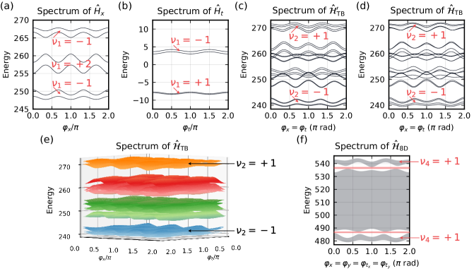
Figure 2: The energy spectra of derived systems. (a) Energy spectrum of the decomposed spatial Hamiltonian $\hat{H}_{x}$. (b) Energy spectrum of the decomposed temporal Hamiltonian $\hat{H}_{t}$. (c) Energy spectrum of $\hat{{\cal H}}^{\prime}_{{\rm TB}}$, equal to the Minkowski sum of the spectra in (a) and (b). A cut of the spectrum along the line $\varphi_{x}=\varphi_{t}$ is shown. (d) Energy spectrum of $\hat{{\cal H}}{}_{{\rm TB}}$ along the line $\varphi_{x}=\varphi_{t}$. (e) Eigenenergy surfaces of $\hat{{\cal H}}{}_{{\rm TB}}$. (f) Energy spectrum of an 8D systems obtained by combining two independent copies of the 4D systems whose spectra are shown in (e). The gray areas represent the bands, with individual levels not shown for visual clarity. The red regions indicate the gaps.

The tight-binding picture. In the basis of the Wannier functions, the Floquet Hamiltonian restricted to the resonant subspace takes the form of the tight-binding model

$$\hat{{\cal H}}_{{\rm TB}}(\varphi_{x},\varphi_{t})=\sum_{\ell^{\prime},\ell}J_{\ell^{\prime}\ell}(\varphi_{x},\varphi_{t})\hat{a}_{\ell^{\prime}}^{\dagger}\hat{a}_{\ell},$$ (4)

where operator $\hat{a}_{i}^{\dagger}$ creates (while $\hat{a}_{i}$ annihilates) a boson on site $\ell$. Here, $\ell\in[1,6Ns]$ enumerates all sites of the 2D time-space lattice, and it is related to the space-time index pair $(j,\alpha)$ as $\ell=2s(j-1)+\alpha$, where $j\in[1,3N]$ and $\alpha\in[1,2s]$. The matrix elements $J_{\ell^{\prime}\ell}$ are calculated as

$$J_{\ell^{\prime}\ell}=\intop_{0}^{sT}\frac{\mathrm{d}t}{sT}\left\langle w_{\ell^{\prime}}\right|\hat{{\cal H}}\left|w_{\ell}\right\rangle,$$ (5)

where $T=2\pi/\omega$ is the driving period. The Wannier basis is constructed repeatedly for every phase $\varphi_{x}$ and $\varphi_{t}$. Each state $\left|w_{\ell}(t)\right\rangle$ is confined to a single spatial site, consequently, only nearest-neighbor spatial couplings are relevant. Moreover, this coupling is appreciable only at times when a given state $\left|w_{\ell}(t)\right\rangle$ is localized near a classical turning point (see the green and yellow states in Fig. 1). At these times, each of these states has only one partner which it is coupled to. Therefore, each Wannier state is coupled to only a single state of those in the neighboring spatial sites. Provided these partners (see like-colored states in Fig. 1) are numbered with the same temporal index $\alpha$, it will not change when a state transitions to a neighboring site (only $j$ will change). This leads to a separable structure of the resulting time-space lattice, where “diagonal” transitions — those which require both indices $j$ and $\alpha$ to change simultaneously — are forbidden. This is an idealized picture, but one which holds with high accuracy since next-nearest-neighbor couplings are negligible (see [28]). Note that this separability is intrinsic to the model described by Eqs. (1)–(3) and cannot be changed by tuning the parameters.

Thus, the Hamiltonian $\hat{{\cal H}}_{{\rm TB}}$ is separable in the sense that

$$\hat{{\cal H}}_{{\rm TB}}\approx\hat{I}_{x}\otimes\hat{H}_{t}+\hat{H}_{x}\otimes\hat{I}_{t}\equiv\hat{{\cal H}}^{\prime}_{{\rm TB}},$$ (6)

where “$\otimes$” denotes the tensor product, $\hat{H}_{x}$ and $\hat{H}_{t}$ are, respectively, the separated spatial and temporal Hamiltonians, while $\hat{I}_{x}$ and $\hat{I}_{t}$ are the identity operators acting in the spaces of, respectively, operators $\hat{H}_{x}$ and $\hat{H}_{t}$. Consequently, the eigenvalue spectrum of $\hat{{\cal H}}^{\prime}_{{\rm TB}}$ is the Minkowski sum of eigenvalue spectra of $\hat{H}_{x}$ and $\hat{H}_{t}$. We will refer to the eigenvalues of all tight-binding Hamiltonians as simply “energies”.

The spectra of $\hat{H}_{x}$ and $\hat{H}_{t}$ are shown in Figs. 2(a) and 2(b) together with the first Chern numbers of each band. Considering the spatial part described by $\hat{H}_{x}$, we treat the phase $\varphi_{x}$ as a fictitious quasimomentum, allowing us to introduce the Berry curvature of the $n$th band, $\Omega_{k_{x}\varphi_{x}}=-2\Im\left\langle\partial_{k_{x}}\chi_{n,k_{x}}|\partial_{\varphi_{x}}\chi_{n,k_{x}}\right\rangle$, and the corresponding first Chern number [39, 40, 41, 8]

$$\nu_{1}^{(x)}=\frac{1}{2\pi}\int_{{\rm BZ}}\mathrm{d}k_{x}\intop_{0}^{2\pi}\mathrm{d}\varphi_{x}\,\Omega_{k_{x}\varphi_{x}}.$$ (7)

In the definition of the Berry curvature, $\left|\chi_{n,k_{x}}\right\rangle$ is the cell-periodic part of the Bloch eigenstate $\mathrm{e}^{\mathrm{i}k_{x}j}\chi_{n,k_{x}}(j)$ of $\hat{H}_{x}$ with $\chi_{n,k_{x}}(j+3)=\chi_{n,k_{x}}(j)$ where $j$ labels spatial sites. For clarity, we suppress indication of the parametric dependence on $\varphi_{x}$ in $\hat{H}_{x}$ and its eigenstates. The crystal momentum $k_{x}$ is treated as a continuous quantity assuming $N\to\infty$. The values of $\nu_{1}^{(x)}$ for the bands shown in Fig. 2(a) may be easily determined as the number of particles of a given band pumped through an arbitrary lattice cross section per pumping cycle (see [28]) or, equivalently, by counting the number of edge state branches in the spectrum of the corresponding non-periodic system [38]. In complete analogy, we introduce the time-quasimomentum $k_{t}$ for the Hamiltonian $\hat{H}_{t}$, so that the eigenstates of $\hat{H}_{t}$ are given by $\mathrm{e}^{\mathrm{i}k_{t}\alpha}\tau_{n,k_{t}}(\alpha)$ with $\tau_{n,k_{t}}(\alpha+2)=\tau_{n,k_{t}}(\alpha)$. The first Chern numbers $\nu_{1}^{(t)}$ of the two bands in Fig. 2(b) are then calculated by integrating the Berry curvature $\Omega_{k_{t}\varphi_{t}}$. Note that by interpreting the phases $\varphi_{x}$ and $\varphi_{t}$ as quasimomenta, we increase the dimensionality of the systems. Each of the Hamiltonians $\hat{H}_{x}$ and $\hat{H}_{t}$ thus describes a 2D system, while their combination, $\hat{{\cal H}}^{\prime}_{{\rm TB}}$, whose spectrum is shown in Fig. 2(c), describes a 4D system. The lowest and the highest bands are nondegenerate and are characterized by the second Chern numbers calculated from the Abelian Berry curvature [8, 9]. Formally, we gather the system parameters into a vector $\boldsymbol{R}=(k_{x},\varphi_{x},k_{t},\varphi_{t})$ and calculate the curvature as $\Omega_{\mu\nu}(\boldsymbol{R})=-2\Im\left\langle\partial_{\mu}\xi_{n,k_{x},k_{t}}|\partial_{\nu}\xi_{n,k_{x},k_{t}}\right\rangle$ where $\partial_{\mu}\equiv\frac{\partial}{\partial R^{\mu}}$, $\mu=1,2,3,4$, and $\left|\xi_{n,k_{x},k_{t}}\right\rangle$ is the cell-periodic part of the $n$th band eigenstate of $\hat{{\cal H}}^{\prime}_{{\rm TB}}$. Due to the factorization $\left|\xi_{n,k_{x},k_{t}}\right\rangle=\left|\chi_{n,k_{x}}\right\rangle\otimes\left|\tau_{n,k_{t}}\right\rangle$, the general formula for the second Chern number [8, 9] reduces to

$$\nu_{2}^{(x,t)}=\frac{1}{4\pi^{2}}\int\mathrm{d}^{4}R\,\Omega_{k_{x}\varphi_{x}}\Omega_{k_{t}\varphi_{t}}=\nu_{1}^{(x)}\nu_{1}^{(t)}.$$ (8)

The values of $\nu_{2}^{(x,t)}$ are indicated in Fig. 2(c).

Comparing the spectrum of $\hat{{\cal H}}^{\prime}{}_{{\rm TB}}$ to the spectrum of the exact tight-binding Hamiltonian $\hat{{\cal H}}{}_{{\rm TB}}$, shown in Fig. 2(d), we note that they are nearly identical. Slight discrepancies are to be expected since in order to obtain the separable Hamiltonian we have neglected some very weak couplings in $\hat{{\cal H}}{}_{{\rm TB}}$ [28]. Nevertheless, the second Chern numbers of the bands of energy spectra of $\hat{{\cal H}}{}_{{\rm TB}}$ and $\hat{{\cal H}}^{\prime}{}_{{\rm TB}}$ are the same. This is supported by the fact that the energy spectrum of $\hat{{\cal H}}_{{\rm TB}}$ can be obtained by adiabatically deforming the spectrum of $\hat{{\cal H}}^{\prime}_{{\rm TB}}$ without closing the gaps in process. Relatedly, we remark that the gap below the highest resonant energy band of $\hat{{\cal H}}_{{\rm TB}}$ remains open for all values of $\varphi_{x}$ and $\varphi_{t}$, as shown in Fig. 2(e). The same is true for the gap above the lowest band of $\hat{{\cal H}}_{{\rm TB}}$.

Higher-dimensional extensions. Finally, let us consider an optical lattice of two orthogonal spatial dimensions, so that the full system Hamiltonian $\hat{H}_{4{\rm D}}=\hat{H}(x,\hat{p}_{x},t|\varphi_{x},\varphi_{t_{x}})+\hat{H}(y,\hat{p}_{y},t|\varphi_{y},\varphi_{t_{y}})$. This produces a 4D time-space crystalline structure since the total Wannier functions now have four independent indices: $W_{\boldsymbol{j},\boldsymbol{\alpha}}(x,y,t)=w_{j_{x},\alpha_{x}}(x,t)w_{j_{y},\alpha_{y}}(y,t)$, where $\boldsymbol{j}=(j_{x},j_{y})$ and $\boldsymbol{\alpha}=(\alpha_{x},\alpha_{y})$ [11]. A two-dimensional temporal structure of $2s\times 2s$ sites now emerges in each two-dimensional spatial cell; motion in the former is characterized by the temporal quasimomenta $k_{t_{x}}$ and $k_{t_{y}}$. The energy spectrum of this system may be readily obtained as a Minkowski sum of two copies of spectra in Fig. 2(e). The result is shown in Fig. 2(f), where it is apparent that the highest and the lowest bands are separated from others by a gap. This holds true not only for the displayed cut of the spectrum at $\varphi_{x}=\varphi_{y}=\varphi_{t_{x}}=\varphi_{t_{y}}$, but rather for all values of the phases. The ratio of the bandwidth of the highest band to the gap below it is found to be 5%, while the ratio of the bandwidth of the lowest band to the gap above it is 2%.

The system whose spectrum is shown in Fig. 2(f) may thus be described by a lattice Hamiltonian

$$\hat{{\cal H}}_{8{\rm D}}=\hat{I}\otimes\hat{{\cal H}}_{{\rm TB}}^{(x)}+\hat{{\cal H}}_{{\rm TB}}^{(y)}\otimes\hat{I},$$ (9)

where $\hat{I}$ is an identity matrix of the same size as $\hat{{\cal H}}_{{\rm TB}}$. The system parameters are the two crystal momenta $k_{x}$, $k_{y}$, the spatial phases $\varphi_{x}$ and $\varphi_{y}$, and the four respective parameters of the two underlying temporal systems: $k_{t_{x}}$, $k_{t_{y}}$, $\varphi_{t_{x}}$, $\varphi_{t_{y}}$. As in the 4D case, the lowest and the highest energy bands are nondegenerate, and therefore may be characterized by the fourth Chern number of a corresponding Abelian gauge field. Generalizing (8) and related equations to 8D in a straightforward way (see [8] and [28] for details), the relevant Chern number results as $\nu_{4}^{(x,t_{x},y,t_{y})}=\nu_{2}^{(x,t_{x})}\nu_{2}^{(y,t_{y})}$. This way we confirm that the highest and the lowest bands in Fig. 2(f) are characterized by nonzero fourth Chern numbers, implying the topologically nontrivial nature of the system. We note that if $\hat{{\cal H}}_{8{\rm D}}$ is constructed using two copies of the approximate Hamiltonian $\hat{{\cal H}}^{\prime}_{{\rm TB}}$, the higher gap closes, whereas the lower one remains open.

It is apparent in Fig. 2(f) that the highest and the lowest bands are wider than the gaps, implying that the gaps disappear if one more copy of the spectrum in Fig. 2(e) is added. Nevertheless, a time-space structure based on a different spatial system than the one given in (2) may exhibit even wider gaps compared to those in Fig. 2(e). This would allow one to realize a 12D time-space structure by combining three copies of $\hat{{\cal H}}_{{\rm TB}}$, each based on a separate physical dimension ($x$, $y$, and $z$).

Conclusions. Summarizing, we have shown that the time-space crystals may be used as a platform for studying 8D systems that can be defined in a tight-binding form. We have devised a concrete, experimentally realizable driven quantum system with validated parameters that is an example of a topologically nontrivial 8D system. Remarkably, it is possible to realize systems with nontrivial topological properties and study the resulting effects in eight dimensions with the help of a properly driven 2D system and without involving any internal degrees of freedom of the particles. High-dimensional spatio-temporal crystalline structures open up possibilities for building practical devices that would be unthinkable in three dimensions. The results presented in this Letter pave the way towards further research in this direction.